Two-time correlation and occupation time for the Brownian bridge and tied-down renewal processes

Abstract

Tied-down renewal processes are generalisations of the Brownian bridge, where an event (or a zero crossing) occurs both at the origin of time and at the final observation time $t$. We give an analytical derivation of the two-time correlation function for such processes in the Laplace space of all temporal variables. This yields the exact asymptotic expression of the correlation in the Porod regime of short separations between the two times and in the persistence regime of large separations. We also investigate other quantities, such as the backward and forward recurrence times, as well as the occupation time of the process. The latter has a broad distribution which is determined exactly. Physical implications of these results for the Poland Scheraga and related models are given. These results also give exact answers to questions posed in the past in the context of stochastically evolving surfaces.

1 Introduction

Tied-down renewal processes with power-law distributions of intervals are generalisations of the Brownian bridge, where an event (or a zero crossing) occurs both at the origin of time and at the final observation time $t$ [1, 2]. The Brownian bridge is itself the continuum limit of the tied-down simple random walk, starting and ending at the origin. The present work is a sequel of our previous study [2] mainly devoted to the statistics of the longest interval of tied-down renewal processes. Here we investigate further quantities of interest such as the two-time correlation function, the backward and forward recurrence times and the occupation time of the process.

The present study parallels that done in [3], where the statistics of these quantities were investigated in the unconstrained case (i.e., without the constraint of having an event at the observation time $t$), then these results were used to give analytical insight in some simplified physical models. The results found here for tied-down renewal processes provide analytical expressions of the pair correlation function in the Porod and persistence regimes and of the distribution of the magnetisation for the Poland Scheraga [5] and related models [6, 7]. They also give exact answers to questions posed in the past in the context of stochastically evolving surfaces [8, 9].

This paper illustrates the importance of a systematic study of renewal processes given their ubiquity and potential applications in statistical physics.

We shall rely on [2] for some background knowledge, in order to keep the present paper short and avoid repeating the material contained in this reference. Nevertheless, we shall start, in section 2, by giving a brief reminder of the most important definitions needed in the subsequent sections 3-6, devoted respectively to the study of the statistics of the forward and backward recurrence times, the number of renewals between two times, the two-time correlation function and finally the occupation time of the process. Section 7 gives applications of the present study to simple equilibrium or nonequilibrium physical systems. Details of some derivations are relegated to appendices.

2 Definitions

2.1 Renewal processes in general

We remind the definitions and notations used for renewal processes, following [3]. Events (or renewals) occur at the random epochs of time $t_{1},t_{2},\ldots$, from some time origin $t=0$. These events are for instance the zero crossings of some stochastic process. We take the origin of time on a zero crossing. When the intervals of time between events, $\tau_{1}=t_{1},\tau_{2}=t_{2}-t_{1},\ldots$, are independent and identically distributed random variables with common density $\rho(\tau)$, the process thus formed is a renewal process [10, 11].

The probability $p_{0}(t)$ that no event occurred up to time $t$ is simply given by the tail probability:

$$p_{0}(t)=\mathop{\rm Prob}\nolimits(\tau_{1}>t)=\int_{t}^{\infty}{\rm d}\tau\,\rho(\tau).$$ (2.1)

The density $\rho(\tau)$ can be either a narrow distribution with all moments finite, in which case the decay of $p_{0}(t)$, as $t\rightarrow\infty$, is faster than any power law, or a distribution characterised by a power-law fall-off with index $\theta>0$

$$p_{0}(t)=\int_{t}^{\infty}{\rm d}\tau\,\rho(\tau)\approx\left(\frac{\tau_{0}}{t}\right)^{\theta},$$ (2.2)

where $\tau_{0}$ is a microscopic time scale. If $\theta<1$ all moments of $\rho(\tau)$ are divergent, if $1<\theta<2$, the first moment $\left\langle\tau\right\rangle$ is finite but higher moments are divergent, and so on. In Laplace space, where $s$ is conjugate to $\tau$, for a narrow distribution we have

$$\mathrel{\mathop{\cal L}\limits_{\tau}}\rho(\tau)=\hat{\rho}(s)=\int_{0}^{\infty}{\rm d}\tau\,\rme^{-s\tau}\rho(\tau)\mathrel{\mathop{=}\limits_{s\rightarrow 0}}1-\left\langle\tau\right\rangle s+\frac{1}{2}\left\langle\tau^{2}\right\rangle s^{2}+\cdots$$ (2.3)

For a broad distribution, (2.2) yields

$$\hat{\rho}(s)\mathrel{\mathop{\approx}\limits_{s\rightarrow 0}}\left\{\begin{array}[]{ll}1-a\,s^{\theta}&(\theta<1)\\ 1-\left\langle\tau\right\rangle s+a\,s^{\theta}&(1<\theta<2),\end{array}\right.\qquad$$ (2.4)

and so on, where

$$a=|\Gamma(1-\theta)|\tau_{0}^{\theta}.$$ (2.5)

From now on, unless otherwise stated, we shall only consider the case $0<\theta<1$.

The quantities naturally associated to a renewal process [3, 10, 11] are the following. The number of events which occurred between $0$ and $t$ (without counting the event at the origin), i.e., the largest $n$ such that $t_{n}\leq t$, is a random variable denoted by $N_{t}$. The time of occurrence of the last event before $t$, that is of the $N_{t}-$th event, is therefore the sum of a random number of random variables

$$t_{N_{t}}=\tau_{1}+\cdots+\tau_{N_{t}}.$$ (2.6)

The backward recurrence time $A_{t}$ is defined as the length of time measured backwards from $t$ to the last event before $t$, i.e.,

$$A_{t}=t-t_{N_{t}}.$$ (2.7)

It is therefore the age of the current, unfinished, interval at time $t$. Finally the forward recurrence time (or excess time) $E_{t}$ is the time interval between $t$ and the next event

$$E_{t}=t_{N_{t}+1}-t.$$ (2.8)

We have the simple relation $A_{t}+E_{t}=t_{N_{t}+1}-t_{N_{t}}=\tau_{N_{t}+1}$. The statistics of these quantities is investigated in detail in [3].

2.2 Tied-down renewal processes

A tied-down renewal process is defined by the condition $\{t_{N_{t}}=t\}$, or equivalently by the condition $\{A_{t}=0\}$, which both express that the $N_{t}-$th event occurred at time $t$. This process generalises the Brownian bridge [2, 1].

The joint density associated to the realisation $\{\ell_{1},\dots,\ell_{n}\}$ of the sequence of $N_{t}=n$ intervals $\{\tau_{1},\dots,\tau_{n}\}$, conditioned by $\{t_{N_{t}}=t\}$, is [2]

$$f^{\star}(t,\ell_{1},\dots,\ell_{n},n)=\frac{\rho(\ell_{1})\dots\rho(\ell_{n})\delta\left(\sum_{i=1}^{n}\ell_{i}-t\right)}{U(t)},$$ (2.9)

where the denominator is obtained from the numerator by integration on the $\ell_{i}$ and summation on $n$,

$$U(t) = \sum_{n\geq 0}\int_{0}^{\infty}{\rm d}\ell_{1}\dots{\rm d}\ell_{n}\,\rho(\ell_{1})\dots\rho(\ell_{n})\delta\Big{(}\sum_{i=1}^{n}\ell_{i}-t\Big{)}.$$ (2.10)

This quantity is the edge value of the probability density of $t_{N_{t}}$ at its maximal value $t_{N_{t}}=t$ [2]. In Laplace space with respect to $t$, we have

$$\hat{U}(s)=\mathrel{\mathop{\cal L}\limits_{t}}U(t)=\sum_{n\geq 0}\hat{\rho}(s)^{n}=\frac{1}{1-\hat{\rho}(s)}.$$ (2.11)

The right side behaves, when $s$ is small, as $s^{-\theta}/a$. Thus, at long times, we finally obtain, using (2.5),

$$U(t)\approx\frac{\sin\pi\theta}{\pi}\frac{t^{\theta-1}}{\tau_{0}^{\theta}}.$$ (2.12)

Knowing the expression (2.9) of the conditional density allows to compute the conditional average of any observable $O$, as

$$\langle O\rangle=\sum_{n\geq 0}\int_{0}^{\infty}{\rm d}\ell_{1}\dots{\rm d}\ell_{n}\,f^{\star}(t,\ell_{1},\dots,\ell_{n},n)\,O.$$ (2.13)

The method used in the next sections consists in computing separately the numerator of this expression, denoted by $\langle O\rangle_{|{\rm num}}$, then divide by the denominator, $U(t)$.

3 Forward and backward recurrence times for the tied-down renewal process

Consider the situation depicted in figure 1. The number of intervals between $0$ and the intermediate time $0<T<t$ is denoted by $N_{T}$. This is also the number of points between 0 and $T$ (without counting the point at the origin). Instead of (2.6) we have now

$$t_{N_{T}}=\tau_{1}+\cdots+\tau_{N_{T}}.$$ (3.1)

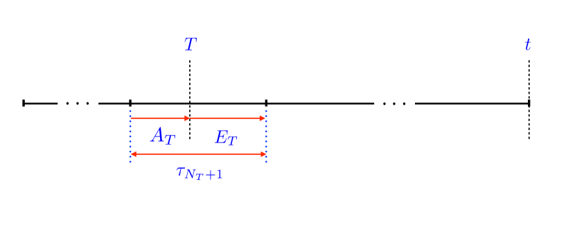
Figure 1: The excess time (or forward recurrence time) $E_{T}$ with respect to $T$ is the distance between $T$ and the next event. The age of the last interval before $T$ (or backward recurrence time) $A_{T}$ is the distance between $t_{N_{t}}$ and $T$. The interval $\tau_{N_{T}+1}$ straddles $T$.

The excess time (or forward recurrence time) with respect to $T$ is, as in (2.8), the time interval between $T$ and the next event

$$E_{T}=t_{N_{T}+1}-T,$$ (3.2)

where $t_{N_{T}+1}=t_{N_{T}}+\tau_{N_{T}+1}$. Its density is

$$f_{E}(t,T,y)=\langle\delta(y-E_{T})\rangle=\frac{{\rm d}}{{\rm d}y}\mathop{\rm Prob}\nolimits(E_{T}<y|t_{N_{t}=t}).$$ (3.3)

In Laplace space, where $s,u,v$ are conjugate to the temporal variables $t,T,y$, we find for the numerator (see A),

$$\hat{f}_{E}(s,u,v){{}_{|{\rm num}}}=\mathrel{\mathop{\cal L}\limits_{t,T,y}}f_{E}(t,T,y){{}_{|{\rm num}}}=\hat{U}(s)\hat{U}(s+u)\frac{\hat{\rho}(s+v)-\hat{\rho}(s+u)}{u-v}.$$ (3.4)

This expression will be used in the next section.

The density $f_{E}(t,T,y)$ is well normalised, as can be seen by noting that

$$\hat{f}_{E}(s,u,0){{}_{|{\rm num}}}=\hat{U}(s)\hat{U}(s+u)\frac{\hat{\rho}(s)-\hat{\rho}(s+u)}{u} = \frac{\hat{U}(s)-\hat{U}(s+u)}{u}$$ (3.5)

$$= \mathrel{\mathop{\cal L}\limits_{t,T}}U(t)\Theta(t-T),$$

where $\Theta$ is the Heaviside function. So, dividing by $U(t)$,

$$\int_{0}^{\infty}{\rm d}y\,f_{E}(t,T,y)=\Theta(t-T).$$ (3.6)

Similarly, one finds for the forward recurrence time $A_{T}=T-t_{N_{T}}$, also named the age of the last interval before $T$ (see B),

$$\hat{f}_{A}(s,u,v){{}_{|{\rm num}}}=\mathrel{\mathop{\cal L}\limits_{t,T,y}}f_{A}(t,T,y){{}_{|{\rm num}}}=\hat{U}(s)\hat{U}(s+u)\frac{\hat{\rho}(s)-\hat{\rho}(s+u+v)}{u+v}.$$ (3.7)

Remark.

The limit $t\to\infty$ ($s\to 0$) corresponds to the unconstrained case. In this limit (3.4) reads

$$\hat{f}_{E}(s\to 0,u,v){{}_{|{\rm num}}}=\hat{U}(s\to 0)\hat{U}(u)\frac{\hat{\rho}(v)-\hat{\rho}(u)}{u-v},$$ (3.8)

which, after Laplace inversion with respect to $s$ and division by $U(t)$, yields, as it should, the expression found for the unconstrained case (see equation (6.2) in [3]) up to the change of $u$ to $s$ and $v$ to $u$. The same holds for $f_{A}$.

4 Number of renewals between two arbitrary times

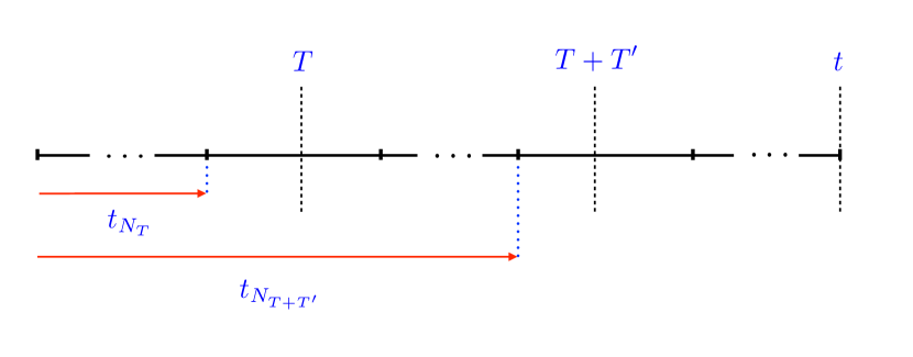
Figure 2: There are $N_{T}$ events up to time $T$ and $N(T,T+T^{\prime})$ events between $T$ and $T+T^{\prime}$.

Consider the number of events $N(T,T+T^{\prime})=N_{T+T^{\prime}}-N_{T}$ occurring between the two times $T$ and $T+T^{\prime}$ (see figure 2). We denote the probability distribution of this random variable by

$$p_{m}(t,T,T+T^{\prime})=\mathop{\rm Prob}\nolimits(N(T,T+T^{\prime})=m|t_{N_{t}}=t).$$ (4.1)

For $m=0$ we have

$$p_{0}(t,T,T+T^{\prime})=\mathop{\rm Prob}\nolimits(E_{T}>T^{\prime})=\int_{T^{\prime}}^{\infty}{\rm d}{y}\,f_{E}(t,T,y).$$ (4.2)

In Laplace space with respect to the three temporal variables $t,T,T^{\prime}$, we find, for $m\geq 1$ (see C),

$$\hat{p}_{m}(s,u,v)_{|{\rm num}} = \mathrel{\mathop{\cal L}\limits_{t,T,T^{\prime}}}p_{m}(t,T,T+T^{\prime})_{|{\rm num}}$$ (4.3)

$$= \hat{f}_{E}(s,u,v)_{|{\rm num}}\frac{\hat{\rho}(s)-\hat{\rho}(s+v)}{v}\hat{\rho}(s+v)^{m-1},$$

and, for $m=0$,

$$\hat{p}_{0}(s,u,v)_{|{\rm num}} = \mathrel{\mathop{\cal L}\limits_{t,T,T^{\prime}}}p_{0}(t,T,T+T^{\prime})_{|{\rm num}}$$ (4.4)

$$= \frac{1}{v}\left(\hat{f}_{E}(s,u,0){{}_{|{\rm num}}}-\hat{f}_{E}(s,u,v){{}_{|{\rm num}}}\right),$$

which is a simple consequence of (4.2) (an alternative proof is given in C). The scaling behaviour of $p_{0}(t,T,T+T^{\prime})$ in the temporal domain is analysed in the next section.

The normalisation of the distribution $p_{m}$ can be checked by computing the sum

$$\sum_{m\geq 0}\hat{p}_{m}(s,u,v)_{|{\rm num}}=\frac{1}{v}\left(\frac{\hat{U}(s)-\hat{U}(s+u)}{u}-\frac{\hat{U}(s+v)-\hat{U}(s+u)}{u-v}\right),$$ (4.5)

the inverse Laplace transform of which is

$$\sum_{m\geq 0}p_{m}(t,T,T+T^{\prime})_{|{\rm num}} = U(t)\Theta(t-T)\Theta(t-T-T^{\prime}),$$ (4.6)

as can be easily checked (see (3.5)). So, finally, after division by $U(t)$,

$$\sum_{m\geq 0}p_{m}(t,T,T+T^{\prime})=\Theta(t-T)\Theta(t-T-T^{\prime}).$$ (4.7)

5 Two-time correlation function

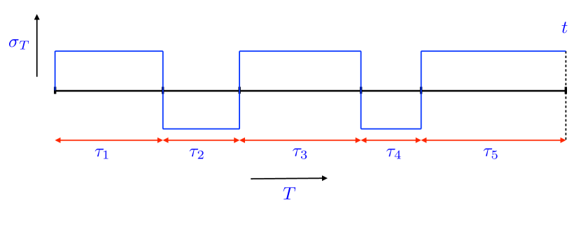
Figure 3: The $\sigma_{T}=\pm 1$ process where $T$ is the running time. In this example the initial condition is $\sigma_{0}=+1$.

In the present section and the next one, we consider the random variable $\sigma_{T}=\pm 1$, where $T$ is the running time, linked to the renewal process as follows. Let $\sigma_{T}=1$, for all the duration of the first interval, then $\sigma_{T}=-1$, during the second interval, and so on, with alternating values, as depicted in figure 3. This process can be thought of as the sign of the position of a one-dimensional underlying motion (such as Brownian motion if $\theta=1/2$). In other words the random variable $\sigma_{T}$ is the sign of the successive excursions (positive if the motion is on the right side of the origin, negative otherwise). We can also interpret $\sigma_{T}$ as a spin variable (depending on time $T$) and the intervals $\tau_{1},\tau_{2},\dots$ as the intervals between two flips [3, 12]. In the present case, the tied-down constraint imposes that the sum of these intervals is given.

5.1 Analytic expression of the two-time correlation function in Laplace space

We want to compute the correlation

$$C(t,T,T+T^{\prime})=\langle\sigma_{T}\sigma_{T+T^{\prime}}\rangle=\langle(-1)^{N(T,T+T^{\prime})}\rangle=\sum_{m\geq 0}(-1)^{m}p_{m}(t,T,T+T^{\prime}),$$ (5.1)

between the two times $T$ and $T+T^{\prime}$. Using the expressions (4.3) and (4.4) above, we obtain, in Laplace space,

$$\hat{C}(s,u,v)_{|{\rm num}}=\frac{1}{v}\left(\hat{f}_{E}(s,u,0)_{|{\rm num}}-\hat{f}_{E}(s,u,v)_{|{\rm num}}\frac{1+\hat{\rho}(s)}{1+\hat{\rho}(s+v)}\right).$$ (5.2)

Taking successively the limits $t\to\infty$, $T\to 0$ and $T^{\prime}\to 0$ allows to check the coherence of the formalism.

1. The limit $t\to\infty$ ($s\to 0$) corresponds to the unconstrained case, as already noted above. We find, after Laplace inversion with respect to $s$ and division by $U(t)$,

   $$\hat{C}(s\to 0,u,v)=\frac{1}{v}\left(\frac{1}{u}-\hat{U}(u)\frac{\hat{\rho}(v)-\hat{\rho}(u)}{u-v}\frac{2}{1+\hat{\rho}(v)}\right).$$ (5.3)

   Changing $u$ to $s$, and $v$ to $u$ in this expression yields equation (9.1) of [3], which is the Laplace transform of the two-time correlation in the unconstrained case.

2. In order to take the limit $T\to 0$, we multiply (5.2) by $u$ then take the limit $u\to\infty$. This yields

   $$\lim_{u\to\infty}u\,\hat{C}(s,u,v)_{|{\rm num}}=\hat{U}(s)\frac{1}{v}\frac{\hat{\rho}(s)-\hat{\rho}(s+v)}{1+\hat{\rho}(s+v)}\equiv\mathrel{\mathop{\cal L}\limits_{t,T^{\prime}}}\langle(-1)^{N_{T^{\prime}}}\rangle_{|{\rm num}},$$ (5.4)

   which, after Laplace inversion and division by $U(t)$, yields the correlation function $\langle\sigma_{0}\sigma_{T^{\prime}}\rangle$.

3. Finally the limit $T^{\prime}\to 0$ is obtained by computing

   $$\lim_{v\to\infty}v\,\hat{C}(s,u,v)_{|{\rm num}}=\hat{f}_{E}(s,u,0)_{|{\rm num}},$$ (5.5)

   which, after Laplace inversion and division by $U(t)$, yields unity as expected.

5.2 Asymptotic analysis in the Porod regime

At large and comparable times $t,T,T^{\prime}$, we have $s\sim u\sim v\ll 1$, hence

$$\hat{C}(s,u,v)_{|{\rm num}}\approx\hat{p}_{0}(s,u,v)_{|{\rm num}},$$ (5.6)

which is given by (4.4). In the present context, $p_{0}(t,T,T+T^{\prime})$ is the probability that the spin $\sigma_{T}$ did not flip between $T$ and $T+T^{\prime}$, or two-time persistence probability. The inversion of the first term in the right side of (4.4) yields $U(t)\Theta(t-T)$, which, after division by $U(t)$ yields 1 (since $t>T$). Let us analyse the second term in the right side of (4.4). In the regime $s\sim u\sim v$ we have

$$\frac{1}{v}\hat{f}_{E}(s,u,v)_{|{\rm num}}\approx\frac{1}{v}\frac{1}{as^{\theta}(s+u)^{\theta}}\frac{(s+u)^{\theta}-(s+v)^{\theta}}{u-v}.$$ (5.7)

Let us moreover focus on the regime of short separations between $T$ and $T+T^{\prime}$, i.e., where $1\ll T^{\prime}\ll T\sim t$. In this regime we expect the following scaling form for the two-time correlation function

$$C(t,T,T+T^{\prime})\approx 1-\left(\frac{T^{\prime}}{t}\right)^{1-\theta}g\left(\frac{T}{t}\right),$$ (5.8)

where the scaling function $g(\cdot)$ is to be determined. In the regime of interest ($s\sim u\ll v$), (5.7) simplifies into

$$\frac{1}{v}\hat{f}_{E}(s,u,v)_{|{\rm num}}\approx\frac{v^{\theta-2}}{as^{\theta}(s+u)^{\theta}}.$$ (5.9)

Laplace inverting the right side of this equation with respect to $v$ yields

$$\frac{T^{\prime 1-\theta}}{a\Gamma(2-\theta)s^{\theta}(s+u)^{\theta}},$$ (5.10)

which, after Laplace inversion with respect to $s$ and $u$ and division by $U(t)$, should be identified with the second term of (5.8), i.e.,

$$\frac{1}{U(t)}\frac{T^{\prime 1-\theta}}{a\Gamma(2-\theta)}\mathrel{\mathop{\cal L}\limits_{s,u}}^{-1}\frac{1}{s^{\theta}(s+u)^{\theta}}=\left(\frac{T^{\prime}}{t}\right)^{1-\theta}g\left(\frac{T}{t}\right).$$ (5.11)

We thus have the following identification to perform

$$\mathrel{\mathop{\cal L}\limits_{s,u}}^{-1}\frac{1}{s^{\theta}(s+u)^{\theta}}={\Gamma(1-\theta)\Gamma(2-\theta)}\frac{\sin\pi\theta}{\pi}t^{2\theta-2}g\left(\frac{T}{t}\right).$$ (5.12)

We have, setting $x=T/t$,

$$\mathrel{\mathop{\cal L}\limits_{t,T}}t^{2\theta-2}g\left(\frac{T}{t}\right) = \int_{0}^{1}{\rm d}x\,g(x)\int_{0}^{\infty}{\rm d}t\,t^{2\theta-1}\rme^{-t(s+ux)}$$ (5.13)

$$= \frac{\Gamma(2\theta)}{s^{2\theta}}\int_{0}^{1}{\rm d}x\,\frac{g(x)}{(1+ux/s)^{2\theta}}.$$

So, using (5.12), we finally obtain the equation determining the scaling function $g(x)$,

$$\int_{0}^{1}{\rm d}x\,\frac{g(x)}{(1+\lambda x)^{2\theta}}=\frac{\Gamma(\theta)}{\Gamma(2-\theta)\Gamma(2\theta)}\frac{1}{(1+\lambda)^{\theta}},$$ (5.14)

with the notation $\lambda=u/s$. Noting that

$$\int_{0}^{1}{\rm d}x\,\frac{\left[x(1-x)\right]^{\theta-1}}{(1+\lambda x)^{2\theta}}=\frac{\Gamma(\theta)^{2}}{\Gamma(2\theta)(1+\lambda)^{\theta}},$$ (5.15)

we conclude that

$$g(x)=\frac{\sin\pi\theta}{\pi(1-\theta)}\left[x(1-x)\right]^{\theta-1},$$ (5.16)

yielding the final result, in the regime of short separations between $T$ and $T+T^{\prime}$ ($1\ll T^{\prime}\ll T\sim t$),

$$C(t,T,T+T^{\prime}) \approx 1-\frac{\sin\pi\theta}{\pi(1-\theta)}\left[\frac{T}{t}\left(1-\frac{T}{t}\right)\right]^{\theta-1}\left(\frac{T^{\prime}}{t}\right)^{1-\theta}$$ (5.17)

$$\approx 1-\frac{\sin\pi\theta}{\pi(1-\theta)}\left(\frac{T^{\prime}t}{T(t-T)}\right)^{1-\theta}.$$

This expression is universal since it no longer depends on the microscopic scale $\tau_{0}$. When $t\to\infty$ we recover the result, easily extracted from [3], for the unconstrained case in the same regime ($1\ll T^{\prime}\ll T$), namely

$$C(T,T+T^{\prime})\approx 1-\frac{\sin\pi\theta}{\pi(1-\theta)}\left(\frac{T^{\prime}}{T}\right)^{1-\theta}.$$ (5.18)

Remark.

Let us apply this formalism to the case of an exponential distribution of intervals, $\rho(\tau)=\lambda\rme^{-\lambda\tau}$ corresponding to a Poisson process for the renewal events. We have, from (5.2),

$$\hat{C}(s,u,v)_{|{\rm num}}=\frac{\lambda}{s(s+u)(s+v+2\lambda)}.$$ (5.19)

By Laplace inversion we obtain

$$C(t,T,T+T^{\prime})=\rme^{-2\lambda T^{\prime}}\Theta(t-T)\Theta(t-T-T^{\prime}),$$ (5.20)

where we used the fact that $U(t)=\lambda$. The correlation is stationary, i.e., a function of $T^{\prime}$ only, as expected. For time differences $T^{\prime}$ such that $\lambda T^{\prime}$ is small, i.e., $T^{\prime}\ll\lambda^{-1}$, this correlation reads $C(T^{\prime})\approx 1-2\lambda T^{\prime}$. Interpreted in the spatial domain, this expression is the usual Porod law [13], where $\lambda$ is the density of defects (domain walls).

5.3 Asymptotic analysis in the persistence regime

Let us now focus on the regime of large separations between $T$ and $T+T^{\prime}$, i.e., where $1\ll T\ll T^{\prime}\sim t$. In this regime we expect the following scaling form for the two-time correlation function

$$C(t,T,T+T^{\prime})\approx p_{0}(t,T,T+T^{\prime})\approx\left(\frac{T^{\prime}}{T}\right)^{-\theta}h\left(\frac{T^{\prime}}{t}\right),$$ (5.21)

where the scaling function $h(\cdot)$ is to be determined. In the regime of interest ($s\sim v\ll u$), (5.7) simplifies into

$$\frac{1}{v}\hat{f}_{E}(s,u,v)_{|{\rm num}}\approx\frac{1}{v}\frac{1}{as^{\theta}u^{\theta}}\frac{u^{\theta}-(s+v)^{\theta}}{u}.$$ (5.22)

Therefore,

$$\hat{p}_{0}(s,u,v)_{|{\rm num}} = \frac{1}{v}\left(\hat{f}_{E}(s,u,0){{}_{|{\rm num}}}-\hat{f}_{E}(s,u,v){{}_{|{\rm num}}}\right)$$ (5.23)

$$\approx \frac{1}{v}\frac{1}{as^{\theta}u^{\theta}}\frac{(s+v)^{\theta}-s^{\theta}}{u}.$$

We proceed as above. Laplace inverting the right side of this equation with respect to $u$ yields

$$\frac{T^{\theta}}{a\Gamma(1+\theta)}\frac{(s+v)^{\theta}-s^{\theta}}{vs^{\theta}},$$ (5.24)

which, after Laplace inversion with respect to $s$ and $v$ and division by $U(t)$, should be identified with the second term of (5.21), i.e.,

$$\frac{1}{U(t)}\frac{T^{\theta}}{a\Gamma(1+\theta)}\mathrel{\mathop{\cal L}\limits_{s,v}}^{-1}\frac{(s+v)^{\theta}-s^{\theta}}{vs^{\theta}}=\left(\frac{T^{\prime}}{T}\right)^{-\theta}h\left(\frac{T^{\prime}}{t}\right).$$ (5.25)

We thus have the following identification to perform

$$\mathrel{\mathop{\cal L}\limits_{s,v}}^{-1}\frac{(s+v)^{\theta}-s^{\theta}}{vs^{\theta}}=\frac{\theta}{t}\left(\frac{T^{\prime}}{t}\right)^{-\theta}h\left(\frac{T^{\prime}}{t}\right).$$ (5.26)

We have, setting $x=T^{\prime}/t$,

$$\mathrel{\mathop{\cal L}\limits_{t,T^{\prime}}}\frac{\theta}{t}\left(\frac{T^{\prime}}{t}\right)^{-\theta}h\left(\frac{T^{\prime}}{t}\right) = \theta\int_{0}^{1}{\rm d}x\,x^{-\theta}h(x)\int_{0}^{\infty}{\rm d}t\,\rme^{-t(s+vx)}$$ (5.27)

$$= \frac{\theta}{s}\int_{0}^{1}{\rm d}x\,\frac{x^{-\theta}h(x)}{1+xv/s}.$$

So, using (5.26), we finally obtain the equation determining the scaling function $h(x)$,

$$\int_{0}^{1}{\rm d}x\,\frac{x^{-\theta}h(x)}{1+\lambda x}=\frac{(1+\lambda)^{\theta}-1}{\lambda},$$ (5.28)

with the notation $\lambda=v/s$. Hence

$$h(x)=\frac{\sin\pi\theta}{\pi\theta}\left(1-x\right)^{\theta},$$ (5.29)

yielding the final result, in the regime of large separations between $T$ and $T+T^{\prime}$ ($1\ll T\ll T^{\prime}\sim t$),

$$C(t,T,T+T^{\prime})\approx p_{0}(t,T,T+T^{\prime}) \approx \frac{\sin\pi\theta}{\pi\theta}\left(\frac{T^{\prime}}{T}\right)^{-\theta}\left(1-\frac{T^{\prime}}{t}\right)^{\theta}$$ (5.30)

$$\approx \frac{\sin\pi\theta}{\pi\theta}\left(\frac{T^{\prime}t}{T(t-T^{\prime})}\right)^{-\theta}.$$

This expression is universal since it no longer depends on the microscopic scale $\tau_{0}$. When $t\to\infty$ we recover the result, easily extracted from [3], for the unconstrained case in the same regime ($1\ll T\ll T^{\prime}$), namely

$$C(T,T+T^{\prime})\approx p_{0}(t,T,T+T^{\prime})\approx\frac{\sin\pi\theta}{\pi\theta}\left(\frac{T^{\prime}}{T}\right)^{-\theta}.$$ (5.31)

5.4 Brownian bridge

For the Brownian bridge, the two-time correlation function (5.1) has an explicit expression. Let $t_{1}$ and $t_{2}$ be two arbitrary times and $x_{t_{1}}$ and $x_{t_{2}}$ the corresponding positions of the process. Then

$$\langle\sigma_{t_{1}}\sigma_{t_{2}}\rangle=\frac{2}{\pi}\arcsin\frac{\langle x_{t_{1}}x_{t_{2}}\rangle}{\sqrt{\langle x_{t_{1}}^{2}\rangle\langle x_{t_{2}}^{2}\rangle}}.$$ (5.32)

For the Brownian bridge between $0$ and $t$, the correlation of positions reads

$$\langle x_{t_{1}}x_{t_{2}}\rangle=\frac{(t-t_{2})t_{1}}{t}.$$ (5.33)

So

$$\langle\sigma_{t_{1}}\sigma_{t_{2}}\rangle=\frac{2}{\pi}\arcsin\sqrt{\frac{t_{1}(t-t_{2})}{t_{2}(t-t_{1})}}.$$ (5.34)

In the present case, $t_{1}\equiv T$, $t_{2}\equiv T+T^{\prime}$. Hence the result

$$C(t,T,T+T^{\prime}) = \frac{2}{\pi}\arcsin\sqrt{\frac{T(t-T-T^{\prime})}{(T+T^{\prime})(t-T)}}$$ (5.35)

$$= 1-\frac{2}{\pi}\arccos\sqrt{\frac{T(t-T-T^{\prime})}{(T+T^{\prime})(t-T)}}.$$

In the regime of short separations between $T$ and $T+T^{\prime}$ ($1\ll T^{\prime}\ll T\sim t$), we obtain

$$C(t,T,T+T^{\prime})\approx 1-\frac{2}{\pi}\sqrt{\frac{T^{\prime}t}{T(t-T)}},$$ (5.36)

which is (5.17) with $\theta=1/2$. In the regime of large separations between $T$ and $T+T^{\prime}$ ($1\ll T\ll T^{\prime}\sim t$), we obtain

$$C(t,T,T+T^{\prime})\approx p_{0}(t,T,T+T^{\prime})\approx\frac{2}{\pi}\sqrt{\frac{T(t-T^{\prime})}{T^{\prime}t}},$$ (5.37)

which is (5.30) with $\theta=1/2$.

6 Occupation time

We turn to an investigation of the occupation time ${\bf T}_{t}$ spent by the process $\sigma_{T}$ in the $(+)$ state up to time $t$, namely

$${\bf T}_{t}=\int_{0}^{t}{\rm d}T\frac{1+\sigma_{T}}{2}.$$ (6.1)

We also consider the more symmetrical quantity

$$S_{t}=\int_{0}^{t}{\rm d}T\,\sigma_{T}=2{\bf T}_{t}-t.$$ (6.2)

We follow the line of thought of [3], which tackles the unconstrained case, in order to analyse these observables. The expression of ${\bf T}_{t}$ depends both on the initial condition $\sigma_{0}$ and on the parity of the number of intervals $N_{t}$. If $\sigma_{0}=+1$, then

$${\bf T}_{t}=\tau_{1}+\tau_{3}+\cdots+\tau_{2k+1}\qquad ({\rm if}\ N_{t}=2k+1)$$ (6.3)

$${\bf T}_{t}=\tau_{1}+\tau_{3}+\cdots+\tau_{2k-1}\qquad ({\rm if}\ N_{t}=2k).$$ (6.4)

The first line is illustrated in figure 3. If $\sigma_{0}=-1$, then

$${\bf T}_{t}=\tau_{2}+\tau_{4}+\cdots+\tau_{2k}\qquad ({\rm if}\ N_{t}=2k+1)$$ (6.5)

$${\bf T}_{t}=\tau_{2}+\tau_{4}+\cdots+\tau_{2k}\qquad ({\rm if}\ N_{t}=2k).$$ (6.6)

The probability density of ${\bf T}_{t}$ is

$$f_{{\bf T}}(t,y)=\langle\delta(y-{\bf T}_{t})\rangle=\sum_{k\geq 0}f_{{\bf T},N_{t}}(t,y,k).$$ (6.7)

In Laplace space, with $s,u$ conjugate to the temporal variables $t,y$, we find, for the numerator, if $\sigma_{0}=+1$,

$$\mathrel{\mathop{\cal L}\limits_{t,y}}f_{{\bf T},N_{t}}(t,y,k){{}_{|{\rm num}}}=\mathrel{\mathop{\cal L}\limits_{t}}\langle\rme^{-u{\bf T}_{t}}\rangle_{|{\rm num}}=\hat{f}_{{\bf T},N_{t}}(s,u,k){{}_{|{\rm num}}}$$ (6.8)

$$=\left\{\begin{array}[]{ll}\hat{\rho}(s+u)^{k+1}\hat{\rho}(s)^{k}&(N_{t}=2k+1)\vspace{12pt}\\ \hat{\rho}(s+u)^{k}\hat{\rho}(s)^{k}&(N_{t}=2k).\end{array}\right.$$ (6.11)

If $\sigma_{0}=-1$,

$$\hat{f}_{{\bf T},N_{t}}(s,u,k){{}_{|{\rm num}}}$$ (6.12)

$$=\left\{\begin{array}[]{ll}\hat{\rho}(s+u)^{k}\hat{\rho}(s)^{k+1}&(N_{t}=2k+1)\vspace{12pt}\\ \hat{\rho}(s+u)^{k}\hat{\rho}(s)^{k}&(N_{t}=2k),\end{array}\right.$$ (6.15)

Summing on $k$, and adding the two contributions corresponding to $\sigma_{0}=\pm 1$ with equal weight $1/2$, we finally find

$$\hat{f}_{{\bf T}}(s,u)_{|{\rm num}}=\frac{1}{1-\hat{\rho}(s)\hat{\rho}(s+u)}\left(1+\frac{\hat{\rho}(s)+\hat{\rho}(s+u)}{2}\right).$$ (6.16)

Let us analyse this expression in the regime, $1\ll t\sim y$, with $y/t=x$ fixed, i.e., such that $s\sim u\ll 1$, with $u/s=\lambda$ fixed. This yields

$$\hat{f}_{{\bf T}}(s,u)_{|{\rm num}}\approx\frac{2}{a\left(s^{\theta}+(s+u)^{\theta}\right)}.$$ (6.17)

This expression should be identified to

$$\mathrel{\mathop{\cal L}\limits_{t,y}}U(t)f_{{\bf T}}(t,y)\mathrel{\mathop{\approx}\limits}\mathrel{\mathop{\cal L}\limits_{t,y}}\frac{U(t)}{t}f_{t^{-1}{\bf T}}(t,x=y/t).$$ (6.18)

In this regime, the limiting density $f_{t^{-1}{\bf T}}(t,x=y/t)$, denoted by $f_{X}(x)$, of the random variable

$$X=\lim_{t\to\infty}t^{-1}{\bf T}_{t},$$ (6.19)

no longer depends on time $t$. So, we are left with the equation for the unknown density $f_{X}(x)$,

$$\frac{2}{a\left(s^{\theta}+(s+u)^{\theta}\right)} = \int_{0}^{\infty}{\rm d}x\,f_{X}(x)\int_{0}^{\infty}{\rm d}t\,\rme^{-t(s+ux)}U(t)$$ (6.20)

$$= \int_{0}^{1}{\rm d}x\,f_{X}(x)\hat{U}(s+ux),$$

that is

$$\int_{0}^{1}{\rm d}x\,\frac{f_{X}(x)}{(1+\lambda x)^{\theta}}=\left\langle\frac{1}{(1+\lambda X)^{\theta}}\right\rangle=\frac{2}{1+(1+\lambda)^{\theta}},$$ (6.21)

where the brackets correspond to averaging on the density $f_{X}(x)$ of $X$. Let us note that $f_{X}(x)$ is well normalised, as can be seen by setting $\lambda=0$ in both sides of the equation. A second remark is that the result obtained is universal since the microscopic scale $\tau_{0}$ is no longer present.

For $\theta=1$ the left side of (6.21) is the usual Stieltjes transform of $f_{X}(x)$, with solution $f_{X}(x)=\delta(x-1/2)$. For $\theta=1/2$, the solution is $f_{X}(x)=1$. We thus recover the well-known result, attributed to Lévy, stating that the occupation time of the Brownian bridge is uniform on $(0,t)$. More generally, the left side of (6.21) is the generalised Stieltjes transform of index $\theta$ of $f_{X}(x)$. A similar equation can be found in [14, 15], in the context of the occupation time of Bessel bridges. Let $F(x)=\int_{0}^{x}{\rm d}u\,f_{X}(u)$. Then $F(x)$ is given by the fractional integral [15]

$$F(x)=\int_{0}^{x}{\rm d}u\,(x-u)^{\theta-1}h(u),$$ (6.22)

where

$$h(u)=\frac{\sin\pi\theta}{\pi}\frac{2u^{\theta}}{u^{2\theta}+(1-u)^{2\theta}+2u^{\theta}(1-u)^{\theta}\cos\pi\theta}\qquad(0<u<1).$$ (6.23)

So the result is

$$f_{X}(x)=\int_{0}^{x}{\rm d}u\,(x-u)^{\theta-1}h^{\prime}(u).$$ (6.24)

This distribution is U-shaped for $\theta<1/2$, and has its concavity inverted for $\theta>1/2$ (see figure 4). It is universal with respect to the choice of distribution of intervals $\rho(\tau)$ as it only depends on the tail exponent $\theta$. For $x\to 0$, the density $f_{X}(x)$ behaves as

$$f_{X}(x)\approx\frac{2\Gamma(1+\theta)}{\Gamma(1-\theta)\Gamma(2\theta)}x^{2\theta-1}.$$ (6.25)

For $\theta<1/2$ the density diverges at the origin, while for $\theta>1/2$ it vanishes.

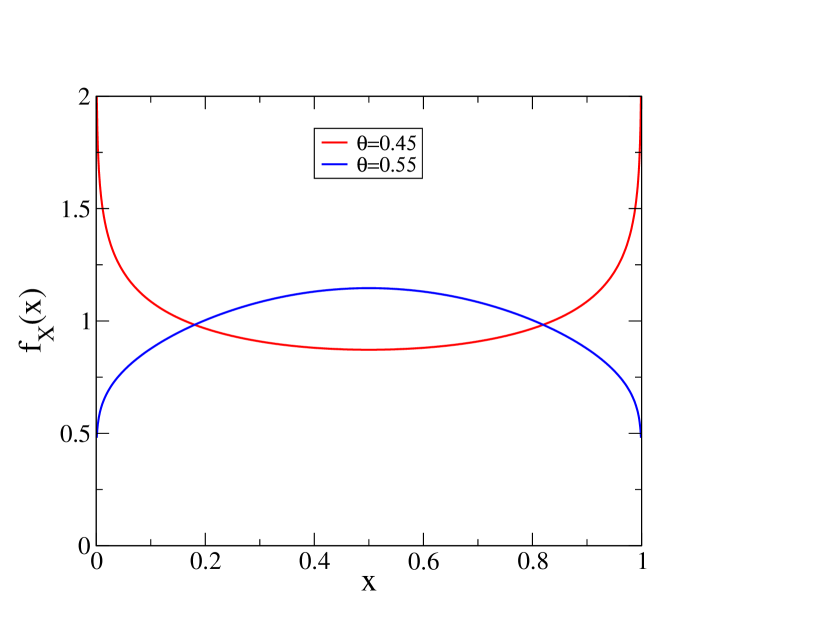
Figure 4: Density of the scaled occupation time $X=\lim_{t\to\infty}t^{-1}{\bf T}_{t}$ for two values of the tail exponent $\theta$, illustrating the change of concavity when crossing $\theta=1/2$ (Brownian bridge). For this latter value the distribution is uniform between $0$ and $1$. The two values of $\theta$ in the figure were chosen not too far from $1/2$ because the further from this value, the more difficult is the numerical evaluation of the distribution of the occupation time.

Expanding the left and right sides of (6.21) yields the moments of the distribution $f_{X}(x)$:

$$\langle X\rangle=\frac{1}{2},\quad\langle X^{2}\rangle=\frac{1}{2(1+\theta)},\quad\langle X^{3}\rangle=\frac{2-\theta}{4(1+\theta)},$$

$$\langle X^{4}\rangle=\frac{3(2-\theta^{2})}{2(1+\theta)(2+\theta)(3+\theta)},$$ (6.26)

and so on. For $\theta=1/2$ one recovers the moments of the uniform distribution on $(0,1)$.

Coming back to the quantity $S_{t}$, we have, using (6.2),

$$\hat{f}_{S}(s,u)=\hat{f}_{{\bf T}}(s-u,2u),$$ (6.27)

so

$$\hat{f}_{S}(s,u)_{|{\rm num}}=\frac{1}{1-\hat{\rho}(s-u)\hat{\rho}(s+u)}\left(1+\frac{\hat{\rho}(s-u)+\hat{\rho}(s+u)}{2}\right).$$ (6.28)

Here $\hat{f}_{S}(s,u)$ is the bilateral Laplace transform of $f_{S}(t,y)$ with respect to $y$ (see [3]) and its usual Laplace transform with respect to $t$. The scaled quantity $M_{t}=t^{-1}S_{t}$ has, when $t\to\infty$, the limiting density

$$f_{M}(m)=\frac{1}{2}f_{X}\left(\frac{1+m}{2}\right),$$ (6.29)

where $-1<m<1$, with vanishing odd moments and

$$\langle M^{2}\rangle=\frac{1-\theta}{1+\theta},\quad\langle M^{4}\rangle=\frac{(1-\theta)(6-5\theta)}{(2+\theta)(3+\theta)},$$ (6.30)

and so on. Considering time as a distance, $M_{t}$ has the interpretation of the magnetisation of a simple spin system, as we shall discuss shortly.

7 In the spatial domain

Let us conclude by interpreting the results derived above in the spatial domain, where time is now considered as a spatial coordinate. In this framework, the tied-down (or pinning) condition is very natural since it amounts to saying that the size of the finite system is fixed.

The $\sigma_{T}$ process defined at the beginning of section 5 now represents a one-dimensional spin system consisting of a fluctuating number $N_{L}$ of spin domains spanning the total size of the system, denoted by $L$ in this context. These domains have lengths $\tau_{i}$, which are discrete random variables with a common distribution denoted by $f_{\ell}=\mathop{\rm Prob}\nolimits(\tau=\ell)$. The probability associated to the realisation $\{\ell_{1},\dots,\ell_{n}\}$ of the sequence of $N_{L}=n$ intervals $\{\tau_{1},\dots,\tau_{n}\}$, is given by the transcription in the spatial domain of (2.9)

$$p(L,\ell_{1},\dots,\ell_{n},n)=\frac{f_{\ell_{1}}\dots f_{\ell_{n}}\delta\left(\sum_{i=1}^{n}\ell_{i},L\right)}{Z(L)},$$ (7.1)

where the Kronecker delta $\delta(i,j)=1$ if $i=j$ and $0$ otherwise. The denominator is

$$Z(L) = \sum_{n\geq 0}\sum_{\ell_{1}\dots\ell_{n}}f_{\ell_{1}}\dots f_{\ell_{n}}\delta\Big{(}\sum_{i=1}^{n}\ell_{i},L\Big{)}.$$ (7.2)

Equation (7.1) can be interpreted as the Boltzmann distribution of an equilibrium model with Hamiltonian (or energy)

$$E(n,\{\ell_{i}\})=-\frac{1}{\beta}\sum_{i=1}^{n}\ln f_{\ell_{i}},$$ (7.3)

where $(n,\{\ell_{i}\})$ is a realisation of the set of observables (number of domains, lengths of domains), with the constraint that the lengths of domains sum up to $L$. In this context, $Z(L)$ is simply the partition function. The expression (7.3) is precisely the energy, at criticality, of the model defined in [6, 7], with the specific choice

$$f_{\ell}=\frac{1}{\zeta(c)}\frac{1}{\ell^{c}},$$ (7.4)

where $c$ plays the role of $1+\theta$ and $\zeta(c)$ is the Riemann zeta function $\zeta(c)=\sum_{\ell\geq 1}\ell^{-c}$. This model is itself a simplified version of the Poland-Scheraga model [5], where the bubbles are seen as spin domains.

The two-time correlation $C(t,T,T+T^{\prime})=\langle\sigma_{T}\sigma_{T+T^{\prime}}\rangle$ becomes the spatial pair correlation function $C(L,x,x+y)=\langle\sigma_{x}\sigma_{x+y}\rangle$ (see figure 5). The scaled quantity $M_{t}$ has the interpretation of the magnetisation of the spin system, i.e., (skipping details about the value of the spin located at the origin),

$$M_{L}=\frac{1}{L}\sum_{i=1}^{N_{L}}(-)^{i}\ell_{i}.$$ (7.5)

The transcription of (5.17) yields the pair correlation function in the Porod regime $y\ll x\sim L$ ($L$ is large)

$$\langle\sigma_{x}\sigma_{x+y}\rangle \approx 1-\frac{\sin\pi\theta}{\pi(1-\theta)}\left[\frac{x}{L}\left(1-\frac{x}{L}\right)\right]^{\theta-1}\left(\frac{y}{L}\right)^{1-\theta}$$ (7.6)

$$\approx 1-\frac{\sin\pi\theta}{\pi(1-\theta)}\left(\frac{yL}{x(L-x)}\right)^{1-\theta}.$$

This expression is universal. Likewise, the probability for two spins at distance $y$ apart to belong to the same domain is given in the persistence regime $x\ll y\sim L$ by the transcription of (5.30), namely

$$p_{0}(L,x,x+y) \approx \frac{\sin\pi\theta}{\pi\theta}\left(\frac{yL}{x(L-y)}\right)^{-\theta},$$ (7.7)

which is also universal.

The transcription of the results of section 6 predicts that the critical magnetisation is fluctuating in the thermodynamical limit, with a broad distribution $f_{M}(m)$ given by (6.29) and (6.24) (see figure 4), whenever the tail exponent $\theta$ of the distribution of domain sizes $f_{\ell}$ is less than one (or $1<c<2$ for the exponent $c$). The distribution $f_{M}(m)$ is universal, i.e., does not depend on the details of $f_{\ell}$. We refer to [2] for a study of the distribution of the number of domains $N_{L}$.

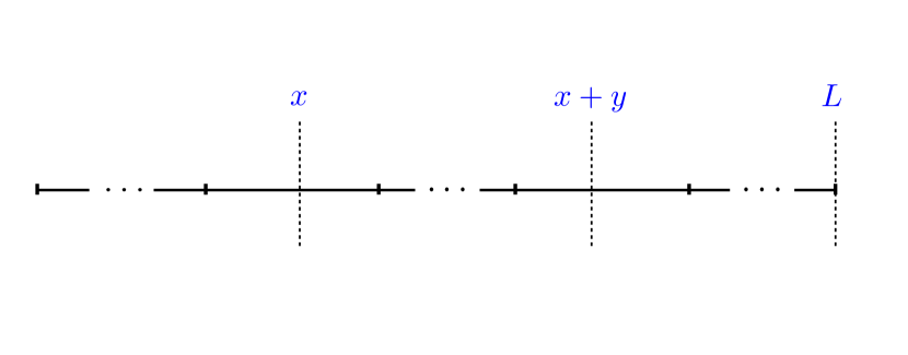
Figure 5: Spatial coordinates defining the pair correlation function $\langle\sigma_{x}\sigma_{x+y}\rangle$.

The results above also provide some answers to issues raised in the past in the field of stochastically evolving surfaces. In [8, 9] coarse-grained depth models for Edwards-Wilkinson and KPZ surfaces are considered. For one of them (the CD2 model in the classification of [8, 9]) the surface profile is related to the tied-down random walk (corresponding to $\theta=1/2$). The expression (7.6) can therefore be interpreted as the pair correlation function of this model in the Porod regime. The prediction $\langle\sigma_{x}\sigma_{x+y}\rangle-1\sim(y/L)^{1-\theta}$ given in [8, 9] for $0<\theta<1$ should also be compared to (7.6). The largest interval for the CD2 model is found in [8, 9] by numerical simulations to satisfy $\tau_{{\rm max}}^{(1)}/L\approx 0.48$, the second largest to satisfy $\tau_{{\rm max}}^{(2)}/L\approx 0.16$. These values are consistent with the analytical predictions $\tau_{{\rm max}}^{(1)}/L\approx 0.483498\ldots$, $\tau_{{\rm max}}^{(2)}/L\approx 0.159987\ldots$ obtained from [2, 16] (see also [17]). Finally, the existence of a broad distribution for the magnetisation of the tied-down renewal process (see (6.29) and (6.24)), which can be seen as a generalisation of the CD2 model with a varying exponent $\theta$, is in line with the expected phenomenology put forward in [8, 9, 18, 19] for fluctuation-dominated phase ordering phenomena. Thus tied-down renewal processes with power-law distribution of intervals are minimal processes implementing a number of the expected characteristics of fluctuation-dominated phase ordering phenomena.

Appendix A Derivation of equation (3.4)

The number $N_{T}$ of events up to time $T$ takes the values $m=0,1,\dots$ and the number $N_{t}$ of events up to time $t$ takes the values $n=m+1,m+2,\dots$ (see figure 1). Consider the probability density

$$f_{E,N_{T},N_{t}}(t,T,m,n,y) = \frac{{{\rm d}}}{{{\rm d}}y}\mathop{\rm Prob}\nolimits(E_{T}<y,N_{T}=m,N_{t}=n|t_{N_{t}}=t)$$ (1.1)

$$= \langle\delta(y-t_{m+1}+T)I(t_{m}<T<t_{m+1})\rangle,$$

where $I(\cdot)$ is the indicator function of the event inside the parentheses. Then by summation upon $m$ and $n$ we get the density of $E_{T}$

$$f_{E}(t,T,y)=\sum_{m\geq 0}\sum_{n\geq m+1}f_{E,N_{T},N_{t}}(t,T,m,n,y).$$ (1.2)

The Laplace transform of (1.1) with respect to $t,T,y$ (with $s,u,v$ conjugate to these variables) reads

$$\mathrel{\mathop{\cal L}\limits_{t,T,y}}f_{E,N_{T},N_{t}}(t,T,m,n,y)=\mathrel{\mathop{\cal L}\limits_{t}}\langle\int_{t_{m}}^{t_{m+1}}{{\rm d}}T\,\rme^{-uT}\rme^{-v(t_{m+1}-T)}\rangle.$$ (1.3)

Its numerator is

$$\mathrel{\mathop{\cal L}\limits_{t,T,y}}f_{E,N_{T},N_{t}}(t,T,m,n,y)_{|{\rm num}} = \int_{0}^{\infty}\left(\prod_{i=1}^{n}{\rm d}\ell_{i}\rho(\ell_{i})\rme^{-s\ell_{i}}\right)\rme^{-vt_{m+1}}\int_{t_{m}}^{t_{m+1}}{{\rm d}}T\,\rme^{-T(u-v)}$$ (1.4)

$$= \hat{\rho}(s+u)^{m}\hat{\rho}(s)^{n-m-1}\frac{\hat{\rho}(s+u)-\hat{\rho}(s+v)}{v-u}.$$

Summing upon $m$ and $n$ yields (3.4).

Setting $v=0$ in (1.4) yields the Laplace transform

$$\mathrel{\mathop{\cal L}\limits_{t,T}}\mathop{\rm Prob}\nolimits(N_{T}=m,N_{t}=n|t_{N_{t}}=t)_{|{\rm num}}=\hat{\rho}(s+u)^{m}\hat{\rho}(s)^{n-m-1}\frac{\hat{\rho}(s)-\hat{\rho}(s+u)}{u}.$$ (1.5)

Summing this expression upon $m$ and $n$ gives back (3.5).

Appendix B Derivation of equation (3.7)

This derivation is very similar to that given above for $f_{E}$. Consider the probability density

$$f_{A,N_{T},N_{t}}(t,T,m,n,y) = \frac{{{\rm d}}}{{{\rm d}}y}\mathop{\rm Prob}\nolimits(A_{T}<y,N_{T}=m,N_{t}=n|t_{N_{t}}=t)$$ (2.1)

$$= \langle\delta(y-T+t_{m})I(t_{m}<T<t_{m+1})\rangle.$$

The Laplace transform of (2.1) with respect to $t,T,y$ (with $s,u,v$ conjugate to these variables) reads

$$\mathrel{\mathop{\cal L}\limits_{t,T,y}}f_{A,N_{T},N_{t}}(t,T,m,n,y)=\mathrel{\mathop{\cal L}\limits_{t}}\langle\int_{t_{m}}^{t_{m+1}}{{\rm d}}T\,\rme^{-uT}\rme^{-v(T-t_{m})}\rangle.$$ (2.2)

Its numerator is

$$\mathrel{\mathop{\cal L}\limits_{t,T,y}}f_{A,N_{T},N_{t}}(t,T,m,n,y)_{|{\rm num}} = \hat{\rho}(s+u)^{m}\hat{\rho}(s)^{n-m-1}\frac{\hat{\rho}(s)-\hat{\rho}(s+u+v)}{u+v}.$$ (2.3)

Summing upon $m$ and $n$ yields (3.7).

Appendix C Derivations of equations (4.3) and (4.4)

Let the number of events $N_{T}$ up to time $T$ take the value $m_{1}$, and the number of events $N(T,T+T^{\prime})=N_{T+T^{\prime}}-N_{T}$ between $T$ and $T+T^{\prime}$ take the value $m_{2}$. We consider the probability of this event (see figure 2)

$$\mathop{\rm Prob}\nolimits(N_{T}=m_{1},N(T,T+T^{\prime})=m_{2},N_{t}=n|t_{N_{t}}=t)$$

$$=\langle I(t_{m_{1}}<T<t_{m_{1}+1})I(t_{m_{1}+m_{2}}<T+T^{\prime}<t_{m_{1}+m_{2}+1})\rangle.$$ (3.1)

Consider first the case $m_{2}\geq 1$. In Laplace space, where $s,u,v$ are conjugate to the temporal variables $t,T,T^{\prime}$, a simple computation gives

$$\mathrel{\mathop{\cal L}\limits_{t,T,T^{\prime}}}\mathop{\rm Prob}\nolimits(N_{T}=m_{1},N(T,T+T^{\prime})=m_{2},N_{t}=n|t_{N_{t}}=t)_{|{\rm num}}$$

$$=\hat{\rho}(s)^{n-m_{1}-m_{2}-1}\hat{\rho}(s+u)^{m_{1}}\frac{\hat{\rho}(s+v)-\hat{\rho}(s+u)}{u-v}\hat{\rho}(s+v)^{m_{2}-1}\frac{\hat{\rho}(s)-\hat{\rho}(s+v)}{v}.$$ (3.2)

Summing on $m_{1}$ from $0$ and on $n$ from $m_{1}+m_{2}+1$ yields

$$\mathrel{\mathop{\cal L}\limits_{t,T,T^{\prime}}}\mathop{\rm Prob}\nolimits(N(T,T+T^{\prime})=m_{2}|t_{N_{t}}=t)_{|{\rm num}}$$

$$=\frac{1}{1-\hat{\rho}(s)}\frac{1}{1-\hat{\rho}(s+u)}\frac{\hat{\rho}(s+v)-\hat{\rho}(s+u)}{u-v}\frac{\hat{\rho}(s)-\hat{\rho}(s+v)}{v}\hat{\rho}(s+v)^{m_{2}-1},$$ (3.3)

which is (4.3) (with $m\equiv m_{2}$).

Consider now the case $m_{2}=0$. We have likewise

$$\mathop{\rm Prob}\nolimits(N_{T}=m_{1},N(T,T+T^{\prime})=0,N_{t}=n|t_{N_{t}}=t)$$

$$=\langle I(t_{m_{1}}<T<t_{m_{1}+1})I(T+T^{\prime}<t_{m_{1}+1})\rangle.$$ (3.4)

In Laplace space, where $s,u,v$ are conjugate to the temporal variables $t,T,T^{\prime}$, a simple computation gives

$$\mathrel{\mathop{\cal L}\limits_{t,T,T^{\prime}}}\mathop{\rm Prob}\nolimits(N_{T}=m_{1},N(T,T+T^{\prime})=0,N_{t}=n|t_{N_{t}}=t)_{|{\rm num}}$$

$$=\hat{\rho}(s)^{n-m_{1}-1}\hat{\rho}(s+u)^{m_{1}}\frac{1}{v}\left[\frac{\hat{\rho}(s)-\hat{\rho}(s+u)}{u}-\frac{\hat{\rho}(s+v)-\hat{\rho}(s+u)}{u-v}\right].$$ (3.5)

Summing on $m_{1}$ from $0$ and on $n$ from $m_{1}+1$ yields

$$\mathrel{\mathop{\cal L}\limits_{t,T,T^{\prime}}}\mathop{\rm Prob}\nolimits(N(T,T+T^{\prime})=0|t_{N_{t}}=t)_{|{\rm num}}$$

$$=\frac{1}{1-\hat{\rho}(s)}\frac{1}{1-\hat{\rho}(s+u)}\frac{1}{v}\left[\frac{\hat{\rho}(s)-\hat{\rho}(s+u)}{u}-\frac{\hat{\rho}(s+v)-\hat{\rho}(s+u)}{u-v}\right],$$ (3.6)

which is (4.4).

References

References

- [1] Wendel J G 1964 Math. Scand. 14 21
- [2] Godrèche C 2017 J. Phys. A 50 195003
- [3] Godrèche C and Luck J M 2001 J. Stat. Phys. 104 489
- [4] Godrèche C, Majumdar S N and Schehr G 2015 J. Stat. Mech. P03014
- [5] Poland D and Scheraga H A 1966 J. Chem. Phys. 45 1464
- [6] Bar A and Mukamel D 2014 Phys. Rev. Lett. 112 015701
- [7] Bar A and Mukamel D 2014 J. Stat. Mech. P11001
- [8] Das D and Barma M 2000 Phys. Rev. Lett. 85 1602
- [9] Das D, Barma M and Majumdar S N 2001 Phys. Rev. E 64 046126
- [10] Cox D R 1962 Renewal theory (London: Methuen)
- [11] Feller W 1968 1971 An Introduction to Probability Theory and its Applications Volumes 1&2 (New York: Wiley)
- [12] Baldassari A, Bouchaud J P, Dornic I and Godrèche C 1999 Phys. Rev. E 59 R20
- [13] Bray A J 1994 Adv. Phys. 43 357
- [14] Yano Y 2006 Publ. RIMS Kyoto Univ. 42 787
- [15] Yano K and Yano Y 2008 Statist. Probab. Lett. 78 2175
- [16] Szabó R and Vetö B 2016 J. Stat. Phys. 165 1086
- [17] Bar A, Majumdar S N, Schehr G and Mukamel D 2016 Phys. Rev. E 93 052130
- [18] Barma M 2008 Eur. Phys. J. B 64 387
- [19] Barma M private communication