Fully computable a posteriori error estimator using anisotropic flux equilibration
on anisotropic meshes

Abstract

Fully computable a posteriori error estimates in the energy norm are given for singularly perturbed semilinear reaction-diffusion equations posed in polygonal domains. Linear finite elements are considered on anisotropic triangulations. To deal with the latter, we employ anisotropic quadrature and explicit anisotropic flux reconstruction. Prior to the flux equilibration, divergence-free corrections are introduced for pairs of anisotropic triangles sharing a short edge. We also give an upper bound for the resulting estimator, in which the error constants are independent of the diameters and the aspect ratios of mesh elements, and of the small perturbation parameter.

1 Introduction

We consider linear finite element approximations to singularly perturbed semilinear reaction-diffusion equations of the form

$$Lu:=-\varepsilon^{2}\triangle u+f(x,y;u)=0\quad\mbox{for}\;\;(x,y)\in\Omega,\qquad u=0\quad\mbox{on}\;\;\partial\Omega,$$ (1.1)

posed in a, possibly non-Lipschitz, polygonal domain $\Omega\subset\mathbb{R}^{2}$. Here $0<\varepsilon\leq 1$. We also assume that $f$ is continuous on $\Omega\times\mathbb{R}$ and satisfies $f(\cdot;s)\in L_{\infty}(\Omega)$ for all $s\in\mathbb{R}$, and the one-sided Lipschitz condition $f(x,y;u)-f(x,y;v)\geq C_{f}[u-v]$ whenever $u\geq v$, with some constant $C_{f}\geq 0$. Then there is a unique $u\in W_{\ell}^{2}(\Omega)\subseteq W_{q}^{1}{\color[rgb]{0,0,0}(\Omega)}\subset C(\bar{\Omega})$ for some $\ell>1$ and $q>2$ [9, Lemma 1]. We additionally assume that $C_{f}+\varepsilon^{2}\geq 1$ (as a division by $C_{f}+\varepsilon^{2}$ immediately reduces (1.1) to this case).

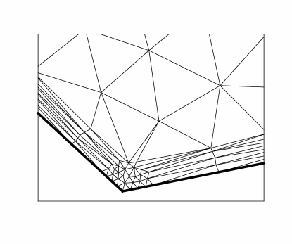
Fig. 1: Example of a mesh that satisfies all assumptions made in §2 (including ${\mathcal{A}}1$ and ${\mathcal{A}}2$).

Our goal is to give explicitly and fully computable a posteriori error estimates on reasonably general anisotropic meshes (such as on Fig. 1 and Fig. 2) in the energy norm defined by

$$\vvvert v\vvvert_{\varepsilon\,;{\Omega}}:=\Bigl{\{}\varepsilon^{2}\|\nabla v\|^{2}_{{\Omega}}+C_{f}\|v\|^{2}_{{\Omega}}\Bigr{\}}^{1/2},$$

where $\color[rgb]{0,0,0}\|\cdot\|_{\mathcal{D}}:=\|\cdot\|_{L_{2}({\mathcal{D}})}\;\forall{\mathcal{D}}\subseteq\Omega$. This goal is achieved by a certain combination of explicit flux reconstruction and flux equilibration.

Flux equilibration for equations of type (1.1) was considered in [1, 3, 4, 7] on shape-regular meshes (see also [2, Chap. 6] for the case $\varepsilon=1$), and in [10] on anisotropic meshes. The estimators in [3, 4, 7] are based on flux reconstructions, while [1, 10] employ solutions of certain local problems.

Our approach in this paper differs from the previous work in a few ways.

• The fluxes are equilibrated within a local patch using anisotropic weights depending on the local, possibly anisotropic, mesh geometry (see (5.3)).

• Prior to the flux equilibration, divergence-free corrections are introduced for pairs of anisotropic triangles sharing a short edge (see §6, in particular, (6.2)).

• A certain anisotropic quadrature is used on anisotropic elements (see §3). This is motivated by some observations made in [13], and also enables us to drop some mesh assumptions made in recent papers [14, 15].

• Our estimator is explicitly and fully computable in the sense that it involves no unknown error constants (unlike other estimators on anisotropic meshes, such as in [10, 14, 15]).

• In contrast to [10], an upper bound for our estimator involves no matching functions (which we discuss below). In fact, the error constant $C$ in the upper bound (1.2) is independent not only of the diameters and the aspect ratios of mesh elements, but also of the small perturbation parameter $\varepsilon$.

• Unlike [1, 3, 4, 7], and also [23, 18, 20, 19], we consider the semilinear case, which mostly simplifies the presentation (as $f$ may include a few linear terms).

• By contrast, dealing with anisotropic elements requires some non-incemental changes in the flux construction and also a more intricate analysis compared to the isotropic-mesh case.

• The efficiency of error estimators on anisotropic meshes was addressed in [18, 20, 19] using the standard bubble function approach. However, a numerical example will be given in §9 that clearly demonstrates that short-edge jump residual terms in such bounds are not sharp. So, under additional restrictions on the anisotropic mesh, we shall give a new bound for the short-edge jump residual terms, and thus show that at least for some anisotropic meshes the error estimator constructed in the paper is efficient.

The robustness of our estimator, denoted by $\mathcal{E}$, with respect to the mesh aspect ratios, as well as the small perturbation parameter $\varepsilon$, is demonstrated by the following upper bound (which follows from Theorems 3 and 5):

$${\mathcal{E}}\leq C\,\Bigl{\{}\sum_{z\in\mathcal{N}}{\color[rgb]{0,0,0}\min\{1,\,\varepsilon h_{z}^{-1}\}}\,\bigl{\|}\varepsilon J_{z}\bigr{\|}^{2}_{\omega_{z}} {}+\sum_{z\in\mathcal{N}}\bigl{\|}\min\{1,\,h_{z}\varepsilon^{-1}\}\,f_{h}^{I}\bigr{\|}^{2}_{\omega_{z}}+\bigl{\|}f_{h}-f_{h}^{I}\bigr{\|}^{2}_{\Omega}\Bigr{.}$$

$$\Bigr{.}+\sum_{T\in\mathcal{T}}\bigl{\|}\lambda_{T}\,{\rm osc}(f_{h}^{I};T)\bigr{\|}^{2}_{T} {}+\!\!\sum_{z\in{\mathcal{N}}^{*}_{\partial\Omega}}\!\bigl{\|}\lambda_{T}f_{h}(z)\bigr{\|}^{2}_{\omega_{z}}\Big{\}}^{1/2},$$ (1.2)

where $C$ is independent of the diameters and the aspect ratios of elements in the triangulation $\mathcal{T}$, and of $\varepsilon$. Here $\mathcal{N}$ is the set of nodes in $\mathcal{T}$, and $\omega_{z}$ is the patch of elements surrounding any $z\in\mathcal{N}$, while $J_{z}$ is the maximum within $\omega_{z}$ of the standard jump in the normal derivative of the computed solution $u_{h}$ across an element edge, $f_{h}=f(\cdot;u_{h})$ and $f_{h}^{I}$ is its standard piecewise-linear Lagrange interpolant. We also use $\lambda_{T}=\min\{1,\,H_{T}\varepsilon^{-1}\}$, $H_{T}\simeq{\rm diam}(T)$, $h_{T}\simeq H_{T}^{-1}|T|$, and $h_{z}\simeq|\omega_{z}|/{\rm diam}(\omega_{z})$ (and some notation defined in the final paragraph of this section). The boundary subset ${\mathcal{N}}^{*}_{\partial\Omega}$ of $\mathcal{N}$ is defined in (2.4).

To relate (1.2) to interpolation error bounds (as well as to possible adaptive-mesh construction strategies), note that $|J_{z}|$ may be interpreted as approximating the diameter of $\omega_{z}$ under the metric induced by the squared Hessian matrix of the exact solution (while $f_{h}^{I}$ approximates $\varepsilon^{2}\triangle u$). Note also that the right-hand side in (1.2) is similar to the estimator in the recent paper [15], and reduces, in the case of shape-regular meshes, to a version of the estimator given by [23].

Explicit residual-type a posteriori error estimates for problems of type (1.1) were also given in [23, 9] on shape-regular meshes, [22, 12, 6] on anisotropic tensor-product meshes, and [18, 20, 19, 14, 15, 16] on more general anisotropic meshes (for $\varepsilon=1$ in [22, 18]). All these estimates are not fully guaranteed in the sense that they involve unknown error constants. (The cited papers deal with the energy norm, except for [6, 9, 12, 14] addressing the maximum norm.)

Note that the error constants in the estimators of [18, 19, 20] (as well as the upper bound for the estimator [10] that we already mentioned) involve the so-called matching functions. The latter depend on the unknown error and take moderate values only when the grid is either isotropic, or, being anisotropic, is aligned correctly to the solution, while, in general, they may be as large as mesh aspect ratios. The presence of such matching functions in the estimator is clearly undesirable, and is entirely avoided in recent papers [14, 15, 16], as well as in our upper bound (1.2).

Finally, note that a posteriori error estimation on anisotropic meshes presents a more serious challenge not only compared to the shape-regular-mesh case, but also to the a priori error estimation. Indeed, there is a vast number of papers showing that a-priori-chosen anisotropic meshes offer an efficient way of computing reliable numerical approximations of solutions that exhibit sharp boundary and interior layers. In the context of singularly perturbed differential equations, such as (1.1) with $\varepsilon\ll 1$, see, for example, [8, 11, 17, 21] and references therein.

The paper is organized as follows. In §2, we list all triangulation assumptions. Next, §3 describes the considered finite element discretization with quadrature. The structure of the reconstructed flux and the main results are presented in §4. The case $h_{z}\lesssim\varepsilon$ is addressed in §§5–6, while §7 deals with the case $h_{z}\gtrsim\varepsilon$. The efficiency of the constructed estimator is illustrated by some numerical results in §8. We conclude the paper by discussing lower error bounds on anisotropic meshes in §9.

Notation. We write $a\simeq b$ when $a\lesssim b$ and $a\gtrsim b$, $a={\mathcal{O}}(b)$ when $|a|\lesssim b$, and $a\lesssim b$ when $a\leq Cb$ with a generic constant $C$ depending on $\Omega$ and $f$, but $C$ does not depend on either $\varepsilon$ or the diameters and the aspect ratios of elements in $\mathcal{T}$. Also, we write $a\ll b$ when $a<c_{0}b$ with a fixed small constant $c_{0}$ (used to distinguish between anisotropic and isotropic elements). The indicator function $\mathbbm{1}_{A}$ takes value $1$ if condition $A$ is satisfied, and vanishes otherwise. For any $\mathcal{D}\subset\Omega$, we let $\|\cdot\|_{\mathcal{D}}=\|\cdot\|_{L_{2}(\mathcal{D})}$, and $\color[rgb]{0,0,0}{\rm osc}(v;\mathcal{D})=\sup_{\mathcal{D}}v-\inf_{\mathcal{D}}v\;\forall v\in L_{\infty}(\mathcal{D})$, while ${\boldsymbol{\nu}}$ and $\boldsymbol{\mu}$, possibly subscripted, denote the unit vectors on $\partial\mathcal{D}$ in the outward normal and counterclockwise tangential direction, respectively. For any triangles $T$ and $T^{\prime}$ sharing an edge, a standard notation is used:

$$\bigl{[}\boldsymbol{\tau}\cdot{\boldsymbol{\nu}}\bigr{]}_{\partial T\cap\partial T^{\prime}}:=\boldsymbol{\tau}\cdot{\boldsymbol{\nu}}\bigr{|}_{T}+\boldsymbol{\tau}\cdot{\boldsymbol{\nu}}\bigr{|}_{T^{\prime}}\,,\qquad\bigl{[}\partial_{\boldsymbol{\nu}}u_{h}\bigr{]}_{\partial T\cap\partial T^{\prime}}:=\bigl{[}\nabla u_{h}\cdot{\boldsymbol{\nu}}\bigr{]}_{\partial T\cap\partial T^{\prime}}\,.$$

2 Triangulation assumptions

We shall use $z$, $S$ and $T$ to respectively denote particular mesh nodes, edges and triangular elements, while $\mathcal{N}$, $\mathcal{S}$ and $\mathcal{T}$ will respectively denote their sets. For each $T\in\mathcal{T}$, let $H_{T}$ be the maximum edge length and $h_{T}:=2H_{T}^{-1}|T|$ be the minimum altitude in $T$. For each $z\in\mathcal{N}$, let $\omega_{z}$ be the patch of elements surrounding any $z\in\mathcal{N}$, ${\mathcal{S}}_{z}$ the set of edges originating at $z$, and

$$H_{z}:={\rm diam}(\omega_{z}),\quad h_{z}:=\max_{T\subset\omega_{z}}h_{T},\quad\mathring{h}_{z}:=\min_{T\subset\omega_{z}}h_{T},\quad\gamma_{z}:={\mathcal{S}}_{z}\setminus\partial\Omega.\vspace{-0.1cm}$$ (2.1)

(With slight abuse of notation, such as in the latter formula, we occasionally treat subsets of $\mathcal{N}$, $\mathcal{S}$ and $\mathcal{T}$ as sets of points.)

Throughout the paper we make some triangulation assumptions. All of them are automatically satisfied by shape-regular triangulations.

• Maximum Angle condition. Let the maximum interior angle in any triangle $T\in\mathcal{T}$ be uniformly bounded by some positive $\lambda_{0}<\pi$.

• Let the number of triangles containing any node be uniformly bounded.

• For any $z\in\mathcal{N}$, one has

  $$h_{T}\simeq\mathring{h}_{z}\;\;\mbox{and}\;\;H_{T}\simeq H_{z}\qquad\mbox{or}\qquad h_{T}\simeq H_{T}\qquad\forall\ T\subset\omega_{z}.$$ (2.2)

Fig. 2: Examples of anisotropic nodes $z\in{\mathcal{N}}_{\rm ani}$ (left), nodes $z\in{\mathcal{N}}\backslash({\mathcal{N}}_{\rm ani}\cup{\mathcal{N}}_{\rm iso})$ (centre), an isotropic node $z\in{\mathcal{N}}_{\rm iso}$ (right), and a node $z\in{\mathcal{N}}_{\partial\Omega}^{*}$ (bottom left). Examples of nodes that satisfy ${\mathcal{A}}1_{\rm ani}^{*}$ (top left), ${\mathcal{A}}1_{\rm ani}$ (bottom left), and ${\mathcal{A}}1_{\rm mix}$ (centre and right).

We also distinguish subsets ${\mathcal{N}}_{\rm ani}$, ${\mathcal{N}}_{\rm iso}$ and ${\mathcal{N}}^{*}_{\partial\Omega}$ of ${\mathcal{N}}$ (see Fig. 2). Note that ${\mathcal{N}}_{\rm ani}\cap{\mathcal{N}}_{\rm iso}=\emptyset$, while ${\mathcal{N}}\backslash({\mathcal{N}}_{\rm ani}\cup{\mathcal{N}}_{\rm iso})$ is not necessarily empty.

(1) Anisotropic nodes, whose set is denoted by ${\mathcal{N}}_{\rm ani}$, are such that

$$h_{z}\ll H_{z},\qquad\quad h_{T}\simeq h_{z}\;\;\mbox{and}\;\;H_{T}\simeq H_{z}\quad\;\forall\ T\subset\omega_{z}.$$ (2.3)

Note that (2.3) implies (2.2), while $z\in{\mathcal{N}}_{\rm ani}$ implies $\mathring{h}_{z}\simeq h_{z}$.

(2) Isotropic nodes, to whose set we shall refer as ${\mathcal{N}}_{\rm iso}$, are such that $h_{z}\simeq H_{z}$.

(3) One may expect anisotropic elements near the boundary to be aligned along it. To distinguish some boundary nodes for which it is not the case, we introduce

$${\mathcal{N}}^{*}_{\partial\Omega}:=\bigl{\{}z\in{\mathcal{N}}_{\rm ani}\cap\partial\Omega\backslash\{\mbox{corners of~{}}\Omega\}\mbox{~{}and~{}}|{\mathcal{S}}_{z}\cap\partial\Omega|\simeq h_{z}\lesssim\varepsilon\bigr{\}}.$$ (2.4)

Occasionally, we shall make additional assumptions that we describe below.

1. Each $z\in\mathcal{N}$ with $h_{z}\lesssim\varepsilon$ satisfies $z\in{\mathcal{N}}_{\rm ani}\backslash\{\mbox{corners of~{}}\Omega\}$ and condition ${\mathcal{A}}1_{\rm ani}$, or it satisfies condition ${\mathcal{A}}1_{\rm mix}$; see below.

2. Quasi-non-obtuse anisotropic elements. Let the maximum triangle angle at $z\in{\mathcal{N}}_{\rm ani}$ be bounded by $\frac{\pi}{2}+\lambda_{1}\frac{h_{z}}{H_{z}}$ for some positive constant $\lambda_{1}$.

3. With $\mathring{\mathcal{S}}_{z}:=\{S\subset{\mathcal{S}}_{z}:|S|\simeq\mathring{h}_{z}\}$ and $\mathring{\omega}_{z}:=\{T\subset\omega_{z}:h_{T}\simeq H_{T}\simeq\mathring{h}_{z}\}$ respectively denoting the sets of edges and isotropic triangles of diameter${}\simeq\mathring{h}_{z}$ within $\omega_{z}$, let $(\mathring{\omega}_{z}\cup\mathring{\mathcal{S}}_{z})\backslash\{z\}$ be connected.

4. Each $z\in\mathcal{N}$ with $h_{z}\gtrsim\varepsilon$ satisfies $\mathring{h}_{z}\geq\sqrt{6}\varepsilon$.

Note that ${\mathcal{A}}1_{\rm ani}$ is always satisfied by isotropic elements, so it requires only some of the anisotropic part of the mesh to be close to a non-obtuse triangulation. ${\mathcal{A}}1_{\rm mix}$ is also always satisfied on shape-regular meshes (as then $\mathring{\omega}_{z}=\omega_{z}$). For anisotropic nodes, ${\mathcal{A}}1_{\rm mix}$ may be satisfied if $z\in\partial\Omega$ (in this case, $\mathring{\omega}_{z}=\emptyset$, while $\mathring{\mathcal{S}}_{z}\backslash\{z\}$ is connected only if $\mathring{\mathcal{S}}$ contains a single edge). Note also that $\mathcal{A}2$ is satisfied for any $z\not\in{\mathcal{N}}_{\rm iso}$, while for isotropic nodes it does impose a mild restriction (as for the latter, $h_{z}\simeq H_{z}$, so whenever $H_{z}\gtrsim\varepsilon$, within $\omega_{z}$ we impose $h_{T}\geq\sqrt{6}\varepsilon$).

We shall also consider a weaker version of ${\mathcal{A}}1$.

1. Each $z\in\mathcal{N}$ with $h_{z}\lesssim\varepsilon$ satisfies $z\in{\mathcal{N}}_{\rm ani}\backslash\partial\Omega$ and condition ${\mathcal{A}}1_{\rm ani}^{*}$, or $z\in{\mathcal{N}}^{*}_{\partial\Omega}$ and satisfies ${\mathcal{A}}1_{\rm ani}$, or it satisfies condition ${\mathcal{A}}1_{\rm mix}$.

2. Local Element Orientation condition. For $z\in\mathcal{N}_{\rm ani}$, there exists a rectangle $R_{z}\supset\omega_{z}$ such that $|R_{z}|\simeq|\omega_{z}|$.

3 Finite element method with quadrature

We discretize (1.1) using linear finite elements. Let $S_{h}\subset H_{0}^{1}(\Omega)\cap C(\bar{\Omega})$ be a piecewise-linear finite element space relative to a triangulation $\mathcal{T}$, and let the computed solution $u_{h}\in S_{h}$ satisfy

$$\varepsilon^{2}\langle\nabla u_{h},\nabla v_{h}\rangle+\langle f_{h},v_{h}\rangle_{h}=0\quad\forall\;v_{h}\in S_{h},\qquad\quad f_{h}(\cdot):=f(\cdot;u_{h}).$$ (3.1)

Here $\langle\cdot,\cdot\rangle$ is the $L_{2}(\Omega)$ inner product, and $\langle\cdot,\cdot\rangle_{h}$ is its quadrature approximation.

We now describe $\langle f_{h},v_{h}\rangle_{h}$ used in (3.1). For the integral over $T\in\mathcal{T}$, a quadrature formula $Q_{T}$ is employed, which is anisotropic on a certain subset ${\mathcal{T}}^{*}$ of anisotropic elements:

$$Q_{T}(w)=|T|\sum_{j=1}^{3}\theta_{T;z_{j}}w(z_{j}):=\left\{\!\begin{array}[]{cl}\frac{1}{3}|T|\bigl{(}w(z_{1})+w(z_{2})+w(z_{3})\bigr{)}&\mbox{for~{}}T\in{\mathcal{T}}\backslash{\mathcal{T}}^{*},\\[5.69046pt] \frac{1}{2}|T|\bigl{(}w(z_{1})+w(z_{2})\bigr{)}&\mbox{for~{}}T\in{\mathcal{T}}^{*}.\end{array}\right.$$ (3.2)

Here $\{z_{j}\}_{j=1}^{3}$ are the vertices of $T$, with $z_{3}=:z^{*}$ opposite the shortest edge, while

$${\mathcal{T}}^{*}:=\{T\in{\mathcal{T}}:h_{T}\ll H_{T}\mbox{~{}and~{}}h_{T}\lesssim\varepsilon\}{}\,\backslash\,{\mathcal{T}}_{0}\,,$$ (3.3)

with ${\mathcal{T}}_{0}\subset\{T\in{\mathcal{T}}:z^{*}\in{\mathcal{N}}_{\rm iso}\mbox{~{}and~{}}z_{1},z_{2}\not\in{\mathcal{N}}_{\rm ani}\backslash\partial\Omega\}$ (so, unless one wants to minimize ${\mathcal{T}}^{*}$, the simplest option is ${\mathcal{T}}_{0}:=\emptyset$). Now, let

$$\langle f_{h},v_{h}\rangle_{h}:=\sum_{T\in{\mathcal{T}}\backslash{\mathcal{T}}^{*}}Q_{T}(f_{h}v_{h})+\sum_{T\in{\mathcal{T}}^{*}}Q_{T}(\widebar{f}_{h}v_{h}),$$ (3.4)

where

$$\widebar{f}_{h}=\bar{f}_{h;T}:={\textstyle\frac{1}{3}}[f_{h}(z_{1})+f_{h}(z_{2})+f_{h}(z_{3})]\quad\forall\ T\in{\mathcal{T}}.$$ (3.5)

As $\widebar{f}_{h}$ is an elementwise constant approximation of $f_{h}$, so $Q_{T}(\bar{f}_{h}v_{h})=\bar{f}_{h,T}Q_{T}(v_{h})$.

Note that the discretization (3.1), (3.2), (3.3), (3.4) can be written as

$$\sum_{S\subset\gamma_{z}}{\textstyle\frac{1}{2}}\varepsilon^{2}|S|\bigl{[}\partial_{\boldsymbol{\nu}}u_{h}\bigr{]}_{S}+\sum_{T\subset\omega_{z}}\theta_{T;z}|T|\,F_{T;z}=0\qquad\forall\ z\in{\mathcal{N}}\backslash\partial\Omega,$$ (3.6)

where $F_{T;z}:=f_{h}(z)$ for $T\in{\mathcal{T}}\backslash{\mathcal{T}}^{*}$ and $F_{T;z}:=\bar{f}_{h;T}$ for $T\in{\mathcal{T}}^{*}$. It will be sometimes convenient to replace the second sum here using an average $\widebar{F}_{z}$ of $F_{T;z}$, associated with $z$, defined by

$$\widebar{F}_{z}\sum_{T\subset\omega_{z}}\!\theta_{T;z}|T|:=\!\sum_{T\subset\omega_{z}}\!\theta_{T;z}|T|\,F_{T;z}\;\;\forall\ z\not\in\partial\Omega,\quad\widebar{F}_{z}:=\color[rgb]{0,0,0}\left\{\!\!\begin{array}[]{cl}0&\!\!\mbox{for}\;z\in{\mathcal{N}}^{*}_{\partial\Omega}:H_{z}\gtrsim\varepsilon,\\ f_{h}(z)&\!\!\mbox{otherwise for}\;z\in\partial\Omega.\end{array}\right.\vspace{0.1cm}$$ (3.7)

Remark 1.

The above quadrature yields the standard linear lumped-mass finite element discretization on ${\mathcal{T}}\backslash{\mathcal{T}}^{*}$. On ${\mathcal{T}}^{*}\!$, a special anisotropic quadrature is employed (designed to address certain convergence issues reported in [13]). The resulting method may be also interpreted as the vertex-centered finite volume method (or the box method) with a special choice of control volumes, applied to the approximation of our equation $-\varepsilon^{2}\triangle u+\widebar{f(\cdot;u)}=0$. A related interpretation as a Petrov-Galerkin method is also possible.

Remark 2.

Our results remain valid, if $Q_{T}(f_{h}v_{h})$ is replaced by $Q_{T}(\widebar{f}_{h}v_{h})$ in the first sum in (3.4). However, using $Q_{T}(f_{h}v_{h})$ for $h_{T}\gg\varepsilon$ yields a superior discretization (as in this case the local stiffness matrices become negligible so diagonal mass matrices are preferable). On the other hand, replacing $Q_{T}(\widebar{f}_{h}v_{h})$ by $Q_{T}(f_{h}v_{h})$ in the second sum in (3.4) yields a less standard lumped-mass discretization on ${\mathcal{T}}^{*}$. For the latter choice, our estimator will enjoy a version of the upper bound (1.2) with $\lambda_{T}$ replaced by $1$ whenever $h_{T}\ll H_{T}\lesssim\varepsilon$. Furthermore, all our results remain valid without any changes if $Q_{T}(\widebar{f}_{h}v_{h})$ is used only for $T\in{\mathcal{T}}^{*}:H_{T}\lesssim\varepsilon$.

4 A posteriori error estimator. Main Results

We start with a relatively standard auxiliary result, a version of which can be found, for example, in [3, Lemma 1] and [7, Theorem 3.1].

Theorem 3.

For any $u_{h}\in S_{h}$, let $\boldsymbol{\tau}\in H^{1}({\rm div},T)\ \forall T\in\mathcal{T}$ also satisfy

$$[\boldsymbol{\tau}\cdot{\boldsymbol{\nu}}]=[\partial_{\boldsymbol{\nu}}u_{h}]\qquad\mbox{on all}\;\;S\in{\mathcal{S}}\backslash\partial\Omega.$$ (4.1)

Then, for a solution $u$ of (1.1), with $C_{f}>0$, one has

$$\vvvert u_{h}-u\vvvert_{\varepsilon\,;\Omega}\leq{\mathcal{E}}:=\Bigl{\{}\|\varepsilon\boldsymbol{\tau}\|_{\Omega}^{2}+C_{f}^{-1}\|\varepsilon^{2}{\rm div}\boldsymbol{\tau}+f_{h}\|_{\Omega}^{2}\Bigr{\}}^{1/2}.$$ (4.2)

Proof.

With $v:=u_{h}-u$, one has

$$\vvvert u_{h}-u\vvvert^{2}_{\varepsilon\,;\Omega} \leq\varepsilon^{2}\langle\nabla(u_{h}-u),\nabla v\rangle+\langle f(\cdot;u_{h})-f(\cdot;u),v\rangle$$

$$=\varepsilon^{2}\langle\nabla u_{h},\nabla v\rangle+\langle f(\cdot;u_{h}),v\rangle\,,$$

$$=\varepsilon^{2}\langle\boldsymbol{\tau},\nabla v\rangle+\langle\varepsilon^{2}{\rm div}\boldsymbol{\tau}+f_{h},v\rangle,$$

which immediately implies (4.2). Here we employed the observation (obtained using $\triangle u_{h}=0$ in any $T$, and (4.1)) that

$$\langle\nabla u_{h},\nabla v\rangle+\langle\underbrace{\triangle u_{h}}_{{}=0},v\rangle=\sum_{S\in\mathcal{S}}\int_{S}v\underbrace{[\partial_{\boldsymbol{\nu}}u_{h}]}_{{}=[\boldsymbol{\tau}\cdot{\boldsymbol{\nu}}]}=\langle\boldsymbol{\tau},\nabla v\rangle+\langle{\rm div}\boldsymbol{\tau},v\rangle.$$

Note that here (as well as in (4.2)), with slight abuse of notation, we understood $\triangle u_{h}$ and ${\rm div}\boldsymbol{\tau}$ as regular functions in $\Omega$ defined elementwise. ∎

Remark 4 (Cases $C_{f}\geq 0$ and $C_{f}=C_{f}(x,y)$).

An inspection of the above proof shows that the estimator ${\mathcal{E}}$ in (4.2) can be replaced by a more general

$${\mathcal{E}}:=\Bigl{\{}(1-\vartheta)^{-1}\|\varepsilon\boldsymbol{\tau}\|_{\Omega}^{2}+\bigl{(}C_{f}+\varepsilon^{2}C_{\Omega}^{-2}\vartheta\bigr{)}^{-1}\|\varepsilon^{2}{\rm div}\boldsymbol{\tau}+f_{h}\|_{\Omega}^{2}\Bigr{\}}^{1/2},$$

where $C_{\Omega}$ is the Poincaré constant, and $\vartheta\in[0,1)$ is an arbitrary constant, with $\vartheta>0$ unless $C_{f}>0$. Note also that if $C_{f}=C_{f}(x,y)$, the above result remains valid with an obvious modification of the energy norm to $\vvvert v\vvvert_{\varepsilon\,;\Omega}:=\bigl{\{}\varepsilon^{2}\|\nabla v\|^{2}_{\Omega}+\|C_{f}^{1/2}v\|^{2}_{\Omega}\bigr{\}}^{1/2}$ and a similar modification of ${\mathcal{E}}$.

4.1 Structure of $\boldsymbol{\tau}$

Clearly, $\boldsymbol{\tau}$ that satisfies the conditions of Theorem 3 is not unique, and there are various choice available in the literature.

Our task in this paper is to explicitly define $\boldsymbol{\tau}$ to be used in (4.2) in a way that is appropriate for anisotropic meshes. We introduce a suitable $\boldsymbol{\tau}$ in the form

$$\boldsymbol{\tau}:=\sum_{z\in\mathcal{N}}\boldsymbol{\tau}_{\!z}+\sum_{T\in{\mathcal{T}}^{\!f}}\boldsymbol{\tau}_{\!T}^{f}+\sum_{S\in{\mathcal{S}}^{*}}\boldsymbol{\tau}_{\!S}^{J},\qquad\quad{\mathcal{T}}^{\!f}:=\{T\in{\mathcal{T}}:H_{T}\lesssim\varepsilon\},$$ (4.3)

where $\boldsymbol{\tau}_{\!z}$, $\boldsymbol{\tau}_{\!T}^{f}$, and $\boldsymbol{\tau}_{\!S}^{J}$ have support on $\omega_{z}$, $T$, and $T\cup T^{\prime}$ for $S=\partial T\cap\partial T^{\prime}$, respectively. It is also convenient to set $\boldsymbol{\tau}_{\!T}^{f}$ and $\boldsymbol{\tau}_{\!S}^{J}$ to $0$ whenever respectively $T\not\in{\mathcal{T}}^{\!f}$ and $S\not\in{\mathcal{S}}^{*}$. Under condition ${\mathcal{A}}1$, we set ${\mathcal{S}}^{*}:=\emptyset$, while otherwise ${\mathcal{S}}^{*}$ is essentially the set of short edges shared by pairs of anisotropic triangles (see §6 for details).

To be more precise, in the case ${\mathcal{S}}^{*}=\emptyset$, the function $\boldsymbol{\tau}_{\!z}$, with support on $\omega_{z}$, is simply required to satisfy

$$[\boldsymbol{\tau}_{\!z}\cdot{\boldsymbol{\nu}}]=\phi_{z}[\partial_{\boldsymbol{\nu}}u_{h}]\;\;\mbox{on}\;\;\gamma_{z},\qquad\quad\boldsymbol{\tau}_{\!z}\cdot{\boldsymbol{\nu}}=0\;\;\mbox{on}\;\;\partial\omega_{z}\backslash\partial\Omega,$$ (4.4)

where $\{\phi_{z}\}_{z\in\mathcal{N}}$ are the standard basis hat functions. The function $\boldsymbol{\tau}_{\!T}$, with support in $T$, satisfies

$$\boldsymbol{\tau}_{\!T}\cdot{\boldsymbol{\nu}}=0\quad\mbox{on}\;\partial T\quad\mbox{and}\quad\varepsilon^{2}{\rm div}\boldsymbol{\tau}_{\!T}+(f_{h}^{I}-\widebar{f}_{h})=0\quad\mbox{in}\;T\qquad\forall\ T\in{\mathcal{T}}^{\!f},$$ (4.5)

and is explicitly defined (see, e.g., [3, (22)]) by

$$\boldsymbol{\tau}_{\!T}^{f}:=b_{1}\phi_{2}\phi_{3}|S_{1}|\boldsymbol{\mu}_{1}+b_{2}\phi_{3}\phi_{1}|S_{2}|\boldsymbol{\mu}_{2}+b_{3}\phi_{1}\phi_{2}|S_{3}|\boldsymbol{\mu}_{3},\qquad{\color[rgb]{0,0,0}b_{j}}:={\textstyle\frac{1}{3}}\varepsilon^{-2}\nabla f_{h}^{I}\cdot|S_{j}|\boldsymbol{\mu}_{j}\,,$$ (4.6)

where $\{z_{j}\}_{j=1}^{3}$ are the vertices of $T$ with the corresponding basis functions $\phi_{j}:=\phi_{z_{j}}$, and for $j=1,2,3$, the edge $S_{j}$ is opposite to $z_{j}$, while the counterclockwise tangential unit vector $\boldsymbol{\mu}_{j}$ lies along $S_{j}$; see Fig. 3.

Fig. 3: Notation used in (4.6): the edge $S_{j}$ is opposite to the vertex $z_{j}$, the counterclockwise tangential unit vector $\boldsymbol{\mu}_{j}$ lies along $S_{j}$.

4.2 Upper bound for the estimator

In this section, we present a theorem, which, combined with (4.2), gives the upper bound (1.2) for the estimator $\mathcal{E}$. At the same time, this theorem provides valuable information on the local properties of the components of $\boldsymbol{\tau}$ in (4.3). These components (except for $\boldsymbol{\tau}_{\!T}^{f}$) are constructed and analyzed in §§5–6 for the case $h_{z}\lesssim\varepsilon$, and in §7 for the case $h_{z}\gtrsim\varepsilon$. So, with the exception of (4.9), all bounds in the following theorem will be obtained in these forthcoming sections. (To be more precise, here we summarize the results of Lemmas 11, 12, 16 and 21.)

Theorem 5.

Let $u_{h}$ solve (3.1) with $\langle\cdot,\cdot\rangle_{h}$ defined in §3, and set

$$J_{z}:=\max_{S\subset\gamma_{z}}\Bigl{|}[\partial_{\boldsymbol{\nu}}u_{h}]_{S}\Bigr{|}\qquad\mbox{and}\qquad\lambda_{T}:=\min\{1,\,H_{T}\varepsilon^{-1}\}\;\;\;\;\forall T\in{\mathcal{T}}\!.$$

(i) Under conditions ${\mathcal{A}}1$ and ${\mathcal{A}}2$, one can construct $\boldsymbol{\tau}$, subject to (4.1), in the form (4.3) with ${\mathcal{S}}^{*}=\emptyset$, where $\boldsymbol{\tau}_{z}$ and an associated function $g_{z}$, both with support in $\omega_{z}$, satisfy, for any $z\in\mathcal{N}$,

$$\sum_{\textstyle{z\in{\mathcal{N}}:{}\above 0.0pth_{z}\lesssim\varepsilon}}\varepsilon^{2}{\rm div}\boldsymbol{\tau}_{\!z}+\widebar{f}_{h}={} \sum_{z\in\mathcal{N}}g_{z}\quad\mbox{in~{}}\Omega,$$ (4.7)

$$\mathbbm{1}_{h_{z}\gtrsim\varepsilon}\,\|\varepsilon^{2}{\rm div}\boldsymbol{\tau}_{\!z}\|_{\omega_{z}}\!+\|\varepsilon\boldsymbol{\tau}_{\!z}\|_{\omega_{z}}\!+\|g_{z}\|_{\omega_{z}}\!\lesssim{} {\color[rgb]{0,0,0}\min\{1,\varepsilon h_{z}^{-1}\}^{1/2}}\|\varepsilon J_{z}\|_{\omega_{z}}\!+\min\{1,h_{z}\varepsilon^{-1}\}\|f_{h}^{I}\|_{\omega_{z}}$$

$$+\!\!\sum_{T\subset\omega_{z}}\!\!\lambda_{T} \|{\rm osc}(f_{h}^{I};T)\|_{T}{}+\mathbbm{1}_{z\in{\mathcal{N}}^{*}_{\partial\Omega}}\,\|\lambda_{T}f_{h}(z)\|_{\omega_{z}},$$ (4.8)

while $\boldsymbol{\tau}_{\!T}^{f}$ from (4.6) satisfies (4.5), and, for any $T\in\mathcal{T}$,

$$\|\varepsilon^{2}{\rm div}\boldsymbol{\tau}^{f}_{T}+(f_{h}-\widebar{f}_{h})\|_{T}+\|\varepsilon\boldsymbol{\tau}^{f}_{T}\|_{T}\lesssim\lambda_{T}\|{\rm osc}(f_{h}^{I};T)\|_{T}+\|f_{h}-f_{h}^{I}\|_{T}.$$ (4.9)

(ii) Under conditions ${\mathcal{A}}1^{*}$ and ${\mathcal{A}}2$, one can construct $\boldsymbol{\tau}$, subject to (4.1), in the form (4.3) with ${\mathcal{S}}^{*}\neq\emptyset$, such that the above relations (4.7), (4.8), (4.9) hold true and, in addition, for any edge $S=\partial T\cap\partial T^{\prime}\in{\mathcal{S}}^{*}$ with an endpoint $z$,

$${\rm div}\boldsymbol{\tau}_{\!S}^{J}=0\;\;\mbox{in~{}}T\cup T^{\prime},\quad\;\;\bigl{\|}\varepsilon\boldsymbol{\tau}_{\!S}^{J}\bigr{\|}_{T\cup T^{\prime}}\lesssim\bigl{\|}\varepsilon[\partial_{\boldsymbol{\nu}}u_{h}]_{S}\bigr{\|}_{T\cup T^{\prime}}\lesssim{\color[rgb]{0,0,0}\min\{1,\,\varepsilon h_{z}^{-1}\}^{1/2}\|\varepsilon J_{z}\|_{\omega_{z}}\,.}$$ (4.10)

Proof of (4.9). If $T\in{\mathcal{T}}^{\!f}$, so, by (4.3), $\lambda_{T}\simeq H_{T}\varepsilon^{-1}$, a calculation [3, §3.3] shows that (4.6) implies (4.5), while $|\gamma_{j}|\lesssim\varepsilon^{-2}{\rm osc}(f_{h}^{I};T)$ yields $|\varepsilon\boldsymbol{\tau}_{\!T}^{f}|\lesssim H_{T}\varepsilon^{-1}{\rm osc}(f_{h}^{I};T)$. The desired bound (4.9) for $T\in{\mathcal{T}}^{\!f}$ follows. Otherwise, i.e. if $T\not\in{\mathcal{T}}^{\!f}$, so $\lambda_{T}\simeq 1$, one has $\boldsymbol{\tau}_{\!T}^{f}=0$, while $|f_{h}-\widebar{f}_{h}|\leq|f_{h}-f_{h}^{I}|+{\rm osc}(f_{h}^{I};T)$, so we again get (4.9).

Remark 6.

Note that for $z\in{\mathcal{N}}^{*}_{\partial\Omega}$, the bound (4.8) involves $\lambda_{T}|f_{h}(z)|\simeq\min\{\varepsilon^{-1},H_{z}^{-1}\}\,H_{z}|f_{h}(z)|$, where $\varepsilon^{-2}H_{z}|f_{h}(z)|$ may be interpreted as the diameter of $\omega_{z}$ under the metric induced by the squared Hessian matrix of the exact solution at $z\in\partial\Omega$. Indeed, as $u=0$ on $\partial\Omega$, the Hessian matrix involves only the normal derivatives, while $\varepsilon^{-2}f_{h}=\varepsilon^{-2}f(\cdot;0)=\partial_{\boldsymbol{\nu}}^{2}u$ on $\partial\Omega$; see also the definition of ${\mathcal{N}}^{*}_{\partial\Omega}$.

5 Construction of $\boldsymbol{\tau}_{z}$ for $h_{z}\lesssim\varepsilon$ under condition ${\mathcal{A}}1$

Let the patch $\omega_{z}$ be formed by $N_{z}$ triangles $\{T_{i}\}_{i=1}^{N_{z}}\subset\mathcal{T}$, numbered counterclockwise so that $\gamma_{z}$ is formed by the edges $\partial T_{i-1}\cap\partial T_{i}$ for $i=1,\ldots,N_{z}$ if $z\not\in\partial\Omega$ (with the notation $T_{0}:=T_{N_{z}}$), and for $i=2,\ldots,N_{z}$ if $z\in\partial\Omega$ (see Fig. 4 (left, centre)). For each $T_{i}\subset\omega_{z}$, let $z$ be opposite to the edge denoted $S_{i}$, with the outward normal and the counterclockwise tangential unit vectors denoted ${\boldsymbol{\nu}}_{i}$ and $\boldsymbol{\mu}_{i}$ (see Fig. 4 (right)).

Define $\boldsymbol{\tau}_{\!z}$ associated with $z$ by

$$\boldsymbol{\tau}_{\!z}:=\phi_{z}\bigl{(}\alpha_{i}{\boldsymbol{\nu}}_{i}+\beta_{i}d_{i}^{-1}\boldsymbol{\mu}_{i}\bigr{)}\quad\forall\ T_{i}\subset\omega_{z},\qquad d_{i}:=2|T_{i}|\,|S_{i}|^{-1},$$ (5.1a)

where, using $$F_{T;z} \widebar{F}_{z}$$ and from (3.6), (3.7),

$${\color[rgb]{0,0,0}\alpha_{i}:=\varepsilon^{-2}d_{i}\theta_{T_{i};z}\widetilde{F}_{T_{i};z},\qquad}\widetilde{F}_{T;z}:=\left\{\begin{array}[]{cl}\widebar{F}_{z}&\mbox{if}\;\;H_{z}\gtrsim\varepsilon\mbox{~{}and~{}}z\in{\mathcal{N}}_{\rm ani},\\ F_{T;z}&\mbox{otherwise}.\end{array}\right.$$ (5.1b)

Here we require $$\{\beta_{i}\}_{i=1}^{N_{z}}$$ to satisfy

$$\beta_{i-1}-\beta_{i}+\alpha_{i-1}{\boldsymbol{\nu}}_{i-1}\cdot|S_{i-1}^{+}|{\boldsymbol{\nu}}^{+}_{i-1}+\alpha_{i}{\boldsymbol{\nu}}_{i}\cdot|S_{i}^{-}|{\boldsymbol{\nu}}^{-}_{i}=|S_{i}^{-}|\bigl{[}\partial_{\boldsymbol{\nu}}u_{h}\bigr{]}_{\partial T_{i-1}\cap\partial T_{i}}$$ (5.1c)

for $$i=1,\ldots,N_{z} z\not\in\partial\Omega i=2,\ldots,N_{z} z\in\partial\Omega S_{i}^{\pm}:=\partial T_{i}\cap\partial T_{i\pm 1} {\boldsymbol{\nu}}^{\pm}_{i} \boldsymbol{\mu}^{\pm}_{i} S_{i}^{\pm} T_{i}$$ if , and for if . We use the notation , as well as and for the outward normal and the counterclockwise tangential unit vectors of the edge in triangle (see Fig. 4 (right)).

Fig. 4: Notation in (5.1): $\omega_{z}$ is formed by $\{T_{i}\}_{i=1}^{N_{z}}$ with $N_{z}=3$ (left) and $N_{z}=5$ (centre); the edge $S_{i}$ in $T_{i}$ is opposite to $z$, with the outward normal and the counterclockwise tangential unit vectors ${\boldsymbol{\nu}}_{i}$ and $\boldsymbol{\mu}_{i}$; the other edges $S_{i}^{\pm}=\partial T_{i}\cap\partial T_{i\pm 1}$ have the outward normal and the counterclockwise tangential unit vectors ${\boldsymbol{\nu}}^{\pm}_{i}$ and $\boldsymbol{\mu}^{\pm}_{i}$ (right).

Lemma 7.

Let $h_{z}\lesssim\varepsilon$. Then relations (5.1) for $\boldsymbol{\tau}_{\!z}$ imply (4.4) and

$$\varepsilon^{2}{\rm div}\boldsymbol{\tau}_{\!z}+\theta_{T;z}\widetilde{F}_{T;z} =0\qquad\forall\ T\subset\omega_{z},$$ (5.2a)

$$\|\varepsilon\boldsymbol{\tau}_{\!z}\|_{\omega_{z}} \lesssim\|h_{z}\varepsilon^{-1}f^{I}_{h}\|_{\omega_{z}}+\varepsilon\,\Bigl{\{}\sum_{i=1}^{N_{z}}\beta^{2}_{i}d_{i}^{-2}|T_{i}|\Bigr{\}}^{1/2}.$$ (5.2b)

The system (5.1c) for $\{\beta_{i}\}_{i=1}^{N_{z}}$ is consistent and has infinitely many solutions.

Proof.

Combining ${\rm div}(\phi_{z}\boldsymbol{\mu}_{i})=\nabla\phi_{z}\cdot\boldsymbol{\mu}_{i}=0$ with ${\rm div}(\phi_{z}{\boldsymbol{\nu}}_{i})=\nabla\phi_{z}\cdot{\boldsymbol{\nu}}_{i}=-d_{i}^{-1}$ one gets ${\rm div}\boldsymbol{\tau}_{\!z}+\alpha_{i}d_{i}^{-1}=0$ in $T_{i}\subset\omega_{z}$, which immediately implies (5.2a). For (5.2b), note that $d_{i}\theta_{T_{i};z}\lesssim h_{z}\theta_{T_{i};z}$, because, in view of (3.2), (3.3), unless $d_{i}\lesssim h_{z}$, one has $T_{i}\in{\mathcal{T}}^{*}$ and $z=z^{*}_{T_{i}}$ so $\theta_{T_{i};z}=0$. Now, $|\varepsilon\alpha_{i}|\lesssim(h_{z}\varepsilon^{-1})\,\theta_{T_{i};z}|\widetilde{F}_{T_{i};z}|$. Combining this with (5.1b) and (3.7), one gets (5.2b)

Next, note that (4.4), combined with (5.1a), is equivalent to

$$\bigl{(}\alpha_{i-1}{\boldsymbol{\nu}}_{i-1}+\beta_{i-1}d_{i-1}^{-1}\boldsymbol{\mu}_{i-1}\bigr{)}\cdot{\boldsymbol{\nu}}^{+}_{i-1}+\bigl{(}\alpha_{i}{\boldsymbol{\nu}}_{i}+\beta_{i}d_{i}^{-1}\boldsymbol{\mu}_{i}\bigr{)}\cdot{\boldsymbol{\nu}}^{-}_{i}=\bigl{[}\partial_{\boldsymbol{\nu}}u_{h}\bigr{]}_{\partial T_{i-1}\cap\partial T_{i}}\,.$$

Multiplying this by $|S_{i-1}^{+}|=|S_{i}^{-}|$ and noting that $d_{i}=\boldsymbol{\mu}_{i}\cdot|S_{i}^{+}|{\boldsymbol{\nu}}^{+}_{i}=-\boldsymbol{\mu}_{i}\cdot|S_{i}^{-}|{\boldsymbol{\nu}}^{-}_{i}$, one gets (5.1c). So (5.1c) is, indeed, equivalent to (4.4).

Finally, consider the system (5.1c) for $\{\beta_{i}\}_{i=1}^{N_{z}}$. For this system to be consistent, it suffices to show that it is under-determined (as then, taking any specific $\beta_{1}$, one can uniquely compute all other $\{\beta_{i}\}$). For $z\in\partial\Omega$, there are $N_{z}-1$ equations, so this system is clearly under-determined. For $z\not\in\partial\Omega$, this is also the case as an application of $\sum_{i=1}^{N_{z}}$ to (5.1c) yields $0$. To check the latter, one first employs the observation that ${\boldsymbol{\nu}}_{i}\cdot\bigl{(}|S_{i}^{+}|{\boldsymbol{\nu}}^{+}_{i}+|S_{i}^{-}|{\boldsymbol{\nu}}^{-}_{i}\bigr{)}+2|T_{i}|d_{i}^{-1}=0$, and then recalls (5.1b), as well as (3.6) and (3.7). ∎

Remark 8 (Anisotropic flux equilibration).

The choice of a particular solution $\{\beta_{i}\}$ of (5.1c) is crucial, as our estimator, roughly speaking, involves the component $\sum_{i=1}^{N_{z}}\beta^{2}_{i}d_{i}^{-2}|T_{i}|$ from (5.2b), while, unless the mesh is shape-regular, $d_{i}^{-2}|T_{i}|=\frac{1}{4}|S_{i}|^{2}|T_{i}|^{-1}$ may vary very significantly within $\omega_{z}$. One simple and useful approach is to minimize this component, i.e. given any particular solution $\{\hat{\beta}_{i}\}$ of (5.1c), let

$$\beta_{i}:=\hat{\beta}_{i}-C_{z},\qquad\mbox{where}\quad\sum_{i}(\hat{\beta}_{i}-C_{z})d_{i}^{-2}|T_{i}|=0.\vspace{-2pt}$$ (5.3)

(Alternatively, one can set $\beta_{i}:=0$ for the element $T_{i}$ with the largest $d_{i}^{-2}|T_{i}|$ within $\omega_{z}$, or choose $\{\beta_{i}\}$ as in the proof of Lemma 12.)

Remark 9 (Computing $\boldsymbol{\tau}_{\!z}$ via optimization).

More generally, for $h_{z}\lesssim\varepsilon$, one can construct $\boldsymbol{\tau}_{\!z}$ using (5.1a) in which $\{\alpha_{i}\}$ and $\{\beta_{i}\}$ are chosen to minimize

$$\sum_{i=1}^{N_{z}}\Bigl{(}{\textstyle\frac{1}{6}}\varepsilon^{2}\alpha_{i}^{2}+{\textstyle\frac{1}{6}}\varepsilon^{2}\beta^{2}_{i}d_{i}^{-2}+[\theta_{T;z}F_{T;z}-\varepsilon^{2}\alpha_{i}d_{i}^{-1}]^{2}\Bigr{)}|T_{i}|\qquad\mbox{subject to \eqref{tau_n_hat}}.\vspace{-0.1cm}$$ (5.4)

(Here we in fact minimize $\|\varepsilon\boldsymbol{\tau}_{\!z}\|^{2}_{\omega_{z}}+\|\varepsilon^{2}{\rm div}\boldsymbol{\tau}_{\!z}+\theta_{T;z}F_{T;z}\|^{2}_{\omega_{z}}$, while (5.1b) is dropped). Then Theorem 5 remains valid (in view of the results in §§5.1–5.2 and §6).

Remark 10.

It is assumed throughout this section that any $z\in{\mathcal{N}}_{\rm ani}$ with $h_{z}\lesssim\varepsilon$ also satisfies $\omega_{z}\subset{\mathcal{T}}^{*}$. This is consistent with the definition (3.3) of ${\mathcal{T}}^{*}$ as long as the somewhat imprecise condition $h_{T}\lesssim\varepsilon$ used in (3.3) always follows from $h_{z}\lesssim\varepsilon$.

5.1 Proof of (4.7) and (4.8) in Theorem 5(i) for $h_{z}\lesssim\varepsilon$

Our findings in this section are presented as two lemmas.

Lemma 11.

Let $\{\boldsymbol{\tau}_{\!z}\}$ satisfy (5.1a), (5.1b) for any $z\in\mathcal{N}$ with $h_{z}\lesssim\varepsilon$. Then for any $z\in{\mathcal{N}}$, there is a function $g_{z}$ with support on $\omega_{z}$ that satisfies (4.7) and (4.8).

Proof.

In any $T\subset\omega_{z}$, let $g_{z}:=\varepsilon^{2}{\rm div}\boldsymbol{\tau}_{\!z}+\theta_{T;z}F_{T;z}$ if $h_{z}\lesssim\varepsilon$, and $g_{z}:=\theta_{T;z}F_{T;z}$ otherwise. In view of (3.2), (3.6), $\sum_{{\mathcal{N}}\cap z\in\partial T}\theta_{T;z}F_{T;z}=\widebar{f}_{h;T}=\widebar{f}_{h}$ in any $T\in\mathcal{T}$, so the first assertion (4.7) follows. Next, if $h_{z}\gtrsim\varepsilon$, i.e. $\min\{1,\,h_{z}\varepsilon^{-1}\}\simeq 1$, one immediately gets $\|g_{z}\|_{\omega_{z}}\lesssim\min\{1,\,h_{z}\varepsilon^{-1}\}\|f_{h}^{I}\|_{\omega_{z}}$. Otherwise, i.e. if $h_{z}\lesssim\varepsilon$, a version of (5.2a) implies $g_{z}=\theta_{T;z}F_{T;z}-\varepsilon^{2}\alpha_{i}d_{i}^{-1}=\theta_{T;z}(F_{T;z}-\widetilde{F}_{T;z})$, and so $|g_{z}|\leq|F_{T;z}-\widetilde{F}_{T;z}|$ for any $T\subset\omega_{z}$. By (5.1b), unless $g_{z}=0$, one has $|g_{z}|\leq|F_{T;z}-\widebar{F}_{z}|\leq{\rm osc}(f_{h}^{I};\omega_{z})+\color[rgb]{0,0,0}\mathbbm{1}_{z\in{\mathcal{N}}^{*}_{\partial\Omega}}f_{h}(z)$, where we also used (3.7). At the same time, $H_{z}\gtrsim\varepsilon$ implies $1\simeq\min\{1,\,H_{z}\varepsilon^{-1}\}\simeq\lambda_{T}$ (as $z\in{\mathcal{N}}_{\rm ani}$ so $H_{z}\simeq H_{T}$). Combining these observations with $|T|\simeq|\omega_{z}|$ for any $T\subset\omega_{z}$ yields $\|g_{z}\|_{\omega_{z}}\lesssim{}$ the second line in (4.8). ∎

Fig. 5: Examples of nodes that satisfy ${\mathcal{A}}1_{\rm mix}$ with the set $\{T_{i}\}_{i=1}^{n}$ (used in the proof of Lemma 12) highlighted by the grey color: $n=5$ (top left), $n=3$ (bottom left), $n=4$ (right).

Lemma 12.

Under condition ${\mathcal{A}}1$, for any $z\in\mathcal{N}$ with $h_{z}\lesssim\varepsilon$, there is a solution $\{\beta_{i}\}_{i=1}^{N_{z}}$ of (5.1c) such that $\boldsymbol{\tau}_{\!z}$ defined by (5.1) satisfies (4.8).

Proof.

Our task is to show that $\|\varepsilon\boldsymbol{\tau}_{\!z}\|_{\omega_{z}}$ satisfies (4.8), in which the right-hand side involves $\color[rgb]{0,0,0}\min\{1,\,\varepsilon h_{z}^{-1}\}\simeq 1$ and $\min\{1,\,h_{z}\varepsilon^{-1}\}\simeq h_{z}\varepsilon^{-1}$. So it suffices to prove

$$\|\varepsilon\boldsymbol{\tau}_{\!z}\|_{\omega_{z}}\lesssim\|\varepsilon J_{z}\|_{\omega_{z}}\!+h_{z}\varepsilon^{-1}\|f^{I}_{h}\|_{\omega_{z}}+\!\!\sum_{T\subset\omega_{z}}\!\!\lambda_{T}\|{\rm osc}(f_{h}^{I};T)\|_{T}+\mathbbm{1}_{z\in{\mathcal{N}}^{*}_{\partial\Omega}}\,\|\lambda_{T}f_{h}(z)\|_{\omega_{z}}.$$ (5.5)

An inspection of the proof of Lemma 7 reveals that if $\widetilde{F}_{T;z}=F_{T;z}$ in (5.1b), then

$$\sum_{T_{i}\subset\omega_{z}}\|\varepsilon\alpha_{i}\|^{2}_{\omega_{z}}\lesssim|\omega_{z}|\,|h_{z}\varepsilon^{-1}f_{h}(z)|^{2}+|\omega_{z}|\!\sum_{\textstyle{T_{i}\in{\mathcal{T}}^{*}:{}\above 0.0ptd_{i}\simeq h_{T_{i}}}}\!\!|d_{i}\varepsilon^{-1}\widebar{f}_{h;T}|^{2}\lesssim\sum_{T\subset\omega_{z}}\|h_{z}\varepsilon^{-1}f^{I}_{h}\|^{2}_{T},$$

where for the first relation we used (3.6) combined with (3.2), (3.3), and for the second, $|\omega_{z}|\simeq h_{z}H_{z}$ and $h_{T_{i}}H_{z}\simeq|T_{i}|$ for any $T_{i}\in{\mathcal{T}}^{*}$. One gets a similar conclusion for the case $\widetilde{F}_{T;z}=\widebar{F}_{z}$ in (5.1b) (in fact, the latter case is more straightforward as then $z\in{\mathcal{N}}_{\rm ani}$ so $|T_{i}|\simeq|\omega_{z}|$ for any $T_{i}\subset\omega_{z}$). Now, in view of (5.2b), to get the desired assertion (5.5), it suffices to show that

$$|\beta_{i}d_{i}^{-1}|\lesssim|J_{z}|+\max_{j=1,\ldots,N_{z}}|\alpha_{j}|+|\hat{\sigma}_{z}|,$$ (5.6)

with some $\hat{\sigma}_{z}$ such that $\|\varepsilon\hat{\sigma}_{z}\|_{\omega_{z}}$ satisfies a version of (5.5).

For (5.6), we start with a straightforward observation that follows from (5.1c):

$$\mbox{if~{}~{}}|S_{i}^{-}|\simeq d_{i}\gtrsim d_{i-1}\quad\Rightarrow\quad|\beta_{i}d_{i}^{-1}|\lesssim|\beta_{i-1}d_{i-1}^{-1}|+|\alpha_{i-1}|+|\alpha_{i}|+|J_{z}|.$$ (5.7)

Consider three cases (a), (b) and (c).

(a) Suppose that $z$ satisfies ${\mathcal{A}}1_{\rm mix}$. Then the $N_{z}$ triangles in $\omega_{z}$ can be numbered counterclockwise so that the set $\{T_{i}\}_{i=1}^{n}\neq\emptyset$, with some $n=n_{z}\leq N_{z}$, is formed by all triangles having at least one edge in $\mathring{S}_{z}$ (see Fig. 5). To be more precise, this set will include all triangles from $\mathring{\omega}_{z}$, and, possibly, one or two anisotropic triangles that either share an edge with $\mathring{\omega}_{z}\neq\emptyset$ or, if $\mathring{\omega}_{z}=\emptyset$ and so $\mathring{S}_{z}$ includes a single edge, touch this edge. Note that then $d_{i}\simeq\mathring{h}_{z}$ for $i=1,\ldots,n_{z}$ and $d_{i}\simeq H_{z}$ for $i>n_{z}$, while $|S_{i}^{-}|\simeq\mathring{h}_{z}$ for $i=2,\ldots,n_{z}$. So setting $\beta_{1}:=0$ and applying (5.7) for $i>1$, we arrive at (5.6) with $\hat{\sigma}_{z}:=0$.

(b) Next, consider $z\in{\mathcal{N}}_{\rm ani}\backslash\partial\Omega$ that satisfies ${\mathcal{A}}1_{\rm ani}$ (and so not ${\mathcal{A}}1_{\rm mix}$). Then $\mathring{\mathcal{S}}_{z}$ includes exactly two edges of length${}\simeq{\mathring{h}}_{z}\simeq h_{z}$. Let the triangles $\{T_{i}\}_{i=1}^{N}$ forming the patch $\omega_{z}$ be numbered counterclockwise so that $\mathring{\mathcal{S}}_{z}=\{\partial T_{i-1}\cap\partial T_{i}\}_{i=1,m+1}$, for some $m=m_{z}\leq N_{z}-2$ (see Fig. 6 (left)).

Note that $d_{i}\simeq h_{z}$ only for $i=0,1,m,m+1$ and $d_{i}\simeq H_{z}$ otherwise, while $|S_{i}^{-}|\simeq h_{z}$ for $i=1,m$ and $\simeq H_{z}$ otherwise. Hence, one can employ (5.7) for $i\neq 0,m$. So it remains to get the desired bound (5.6) only for $i=0,m$. For this, let

$$\widetilde{\sigma}_{z}:=\sum_{i=2}^{m}|S_{i}^{-}|\bigl{[}\partial_{\boldsymbol{\nu}}u_{h}\bigr{]}_{\partial T_{i-1}\cap\partial T_{i}}+2\varepsilon^{-2}\sum_{i=1}^{m}\theta_{T_{i};z}|T_{i}|\,\widetilde{F}_{T_{i};z}$$ (5.8)

(compare with (3.6)). Now, an application of $\sum_{i=1}^{m}$ to (5.1c) (and also noting that ${\boldsymbol{\nu}}_{i}\cdot\bigl{(}|S_{i}^{+}|{\boldsymbol{\nu}}^{+}_{i}+|S_{i}^{-}|{\boldsymbol{\nu}}^{-}_{i}\bigr{)}+2|T_{i}|d_{i}^{-1}=0$) yields

$$\beta_{0}-\beta_{m}+\alpha_{0}{\boldsymbol{\nu}}_{0}\cdot|S_{0}^{+}|{\boldsymbol{\nu}}^{+}_{0}-\alpha_{m}{\boldsymbol{\nu}}_{m}\cdot|S_{m}^{+}|{\boldsymbol{\nu}}^{+}_{m}=|S_{1}^{-}|\bigl{[}\partial_{\boldsymbol{\nu}}u_{h}\bigr{]}_{\partial T_{0}\cap\partial T_{1}}+\widetilde{\sigma}_{z}.$$ (5.9)

So, for example, one can set $\beta_{0}:=0$ and compute and then estimate $\beta_{m}$ from (5.9). Or, one can choose $\beta_{0}$ and $\beta_{m}$, in agreement with (5.9), but in a more balanced way. Importantly, one can ensure for $i=0,m$ that $|\beta_{i}d_{i}^{-1}|\lesssim|\alpha_{i}|+|J_{z}|+h_{z}^{-1}|\widetilde{\sigma}_{z}|$. Consequently, we get (5.6) for all $i$ with $\hat{\sigma}_{z}:=h_{z}^{-1}\widetilde{\sigma}_{z}$.

Finally, similarly to (3.7), define a version of (5.8):

$$\sigma_{z}:=\sum_{i=2}^{m}|S_{i}^{-}|\bigl{[}\partial_{\boldsymbol{\nu}}u_{h}\bigr{]}_{\partial T_{i-1}\cap\partial T_{i}}+2\varepsilon^{-2}\widebar{F}_{z}\sum_{i=1}^{m}\theta_{T_{i};z}|T_{i}|.$$ (5.10)

By (5.1b), unless $\widetilde{\sigma}_{z}=\sigma_{z}$, one has $\widetilde{F}_{T_{i};z}\neq\widebar{F}_{z}$ and so $H_{z}\varepsilon^{-1}\simeq\min\{1,\,H_{z}\varepsilon^{-1}\}\simeq\lambda_{T}$ (the latter is also because $z\in{\mathcal{N}}_{\rm ani}$), so $\varepsilon h_{z}^{-1}|\widetilde{\sigma}_{z}-\sigma_{z}|\lesssim\sum_{T\subset\omega_{z}}\lambda_{T}\,{\rm osc}(f_{h}^{I};T)$. Combining this with a technical result (5.13) (obtained below in §5.2), one arrives at

$$|\varepsilon h_{z}^{-1}\widetilde{\sigma}_{z}|=|\varepsilon\hat{\sigma}_{z}|\lesssim|\varepsilon J_{z}|+h_{z}\varepsilon^{-1}|\widebar{F}_{z}|+\sum_{T\subset\omega_{z}}\lambda_{T}\,{\rm osc}(f_{h}^{I};T).$$ (5.11)

As $\|\widebar{F}_{z}\|_{\omega_{z}}\lesssim\|f_{h}^{I}\|_{\omega_{z}}$ (by (3.6), (3.7)), so we have again obtained (5.6) with $\|\varepsilon\hat{\sigma}_{z}\|_{\omega_{z}}$ now satisfying a version of (5.5). This completes the proof of (5.5) for this case.

(c) It remains to consider $z\in{\mathcal{N}}^{*}_{\partial\Omega}$, which satisfies ${\mathcal{A}}1_{\rm ani}$ but not ${\mathcal{A}}1_{\rm mix}$. This case is similar to case (b), with a version of (5.9) becoming

$$\beta_{1}-\beta_{m}-\alpha_{1}{\boldsymbol{\nu}}_{1}\cdot|S_{1}^{-}|{\boldsymbol{\nu}}^{-}_{1}-\alpha_{m}{\boldsymbol{\nu}}_{m}\cdot|S_{m}^{+}|{\boldsymbol{\nu}}^{+}_{m}=\widetilde{\sigma}_{z}.$$

Again, using (5.13), we get a version of (5.11) with an additional term $H_{z}\varepsilon^{-1}|\widebar{F}_{z}|$ in the right-hand side. As, by (3.7), unless $\widebar{F}_{z}=0$, one has $\widebar{F}_{z}=f_{h}(z)$ and $H_{z}\varepsilon^{-1}\simeq\min\{1,\,H_{z}\varepsilon^{-1}\}\simeq\lambda_{T}$ for $z\in{\mathcal{N}}^{*}_{\partial\Omega}$, we again get (5.5). ∎

5.2 Estimation of $\sigma_{z}$

Here we give one technical result on $\sigma_{z}$. Throughout this section, we use the notation from the proof of Lemma 12.

Lemma 13.

(i) If $z\in{\mathcal{N}}_{\rm ani}\backslash\partial\Omega$, with $h_{z}\lesssim\varepsilon$, satisfies ${\mathcal{A}}1_{\rm ani}^{*}$, then for $\sigma_{z}$ of (5.10) one has

$$\varepsilon h_{z}^{-1}\bigg{|}\sigma_{z}-\!\!\!\sum_{i=1,m+1}\boldsymbol{\mu}_{i-1}^{+}\cdot{\mathbf{i}}_{\xi}\,\,\frac{H_{T_{i-1}}H_{T_{i}}}{H_{T_{i-1}}+H_{T_{i}}}\,[\partial_{\boldsymbol{\nu}}u_{h}]_{\partial T_{i-1}\cap\partial T_{i}}\bigg{|}\lesssim|\varepsilon J_{z}|+h_{z}\varepsilon^{-1}|\widebar{F}_{z}|,$$ (5.12)

where $\mathbf{i}_{\xi}$ is the unit vector that points from $z$ in the direction of any edge from $\{S_{i}^{-}\}_{i=2}^{m}$.

(ii) If $z\in{\mathcal{N}}_{\rm ani}\backslash\{\mbox{corners of~{}}\Omega\}$, with $h_{z}\lesssim\varepsilon$, satisfies ${\mathcal{A}}1_{\rm ani}$ but not ${\mathcal{A}}1_{\rm mix}$, then

$$\varepsilon h_{z}^{-1}|\sigma_{z}|\lesssim|\varepsilon J_{z}|+h_{z}\varepsilon^{-1}|\widebar{F}_{z}|+\mathbbm{1}_{z\in{\mathcal{N}}^{*}_{\partial\Omega}}\,\,H_{z}\varepsilon^{-1}|\widebar{F}_{z}|.$$ (5.13)

Proof.

(i) For any scalar $w$, let $\llbracket w\rrbracket_{\partial T_{i-1}\cap\partial T_{i}}:=w\bigr{|}_{\partial T_{i}}-w\bigr{|}_{\partial T_{i-1}}$. Furthermore, for fixed $z\in\mathcal{N}$, introduce the local cartesian coordinates $(\xi,\eta)$ such that $z=(0,0)$, and ${\mathbf{i}}_{\xi}$ points in the $\xi$ direction (see Fig. 6 (left)). In these coordinates, let $(\xi_{i},\eta_{i})$ be the endpoint of the edge $S_{i}^{-}=\partial T_{i-1}\cap\partial T_{i}$ on $\partial\omega_{z}$.

Now, a calculation shows that $|S_{i}^{-}|\bigl{[}\partial_{\boldsymbol{\nu}}u_{h}\bigr{]}_{\partial T_{i-1}\cap\partial T_{i}}=\eta_{i}\llbracket\partial_{\xi}u_{h}\rrbracket-\xi_{i}\llbracket\partial_{\eta}u_{h}\rrbracket$, where, by ${\mathcal{A}}^{*}_{\rm ani}$ and the maximum angle condition, any $|\eta_{i}|\lesssim h_{z}$, while $\displaystyle H_{z}^{+}:=\min_{i=2,\ldots m}\xi_{i}\simeq H_{z}$ and $0\leq\xi_{i}-H_{z}^{+}\lesssim h_{z}$, so

$$\sigma_{z}=-\sum_{i=2}^{m}H_{z}^{+}\llbracket\partial_{\eta}u_{h}\rrbracket_{\partial T_{i-1}\cap\partial T_{i}}+{\mathcal{O}}(h_{z}|J_{z}|)+\varepsilon^{-2}\widebar{F}_{z}\!\sum_{i=1,m}\!\!\!|T_{i}|.$$ (5.14)

Here we also used $\theta_{T_{i};z}=0$ for $i=2,\ldots,m-1$ and $\theta_{T_{i};z}=\frac{1}{2}$ for $i=1,m$ in view of $T_{i}\subset{\mathcal{T}}^{*}$ for any $T_{i}\subset\omega_{z}$ (see also (3.2), (3.3)).

Next, multiplying (3.6) combined with (3.7) by $2\varepsilon^{-2}$, then subtracting $\sigma_{z}$ and applying a similar argument, one gets

$$-\sigma_{z}=\sum_{i=m+2}^{N}H_{z}^{-}\llbracket\partial_{\eta}u_{h}\rrbracket_{\partial T_{i-1}\cap\partial T_{i}}+{\mathcal{O}}(h_{z}|J_{z}|)+\varepsilon^{-2}\widebar{F}_{z}\!\!\!\!\sum_{i=m+1,N}\!\!\!\!|T_{i}|.$$ (5.15)

Here $\displaystyle H_{z}^{-}:=\min_{i=m+2,\ldots N}|\xi_{i}|\simeq H_{z}$, and we also used $|S_{i}^{-}|\simeq h_{z}$ for $i=1,m+1$.

Finally, using $|T_{1}|=\frac{1}{2}|\xi_{2}\eta_{1}-\xi_{1}\eta_{2}|=\frac{1}{2}\eta_{1}H_{z}^{+}+{\mathcal{O}}(h_{z}^{2})$ (where $|\xi_{1}|+|\eta_{2}|\lesssim h_{z}$) and similar observations for the other triangle areas, we arrive at

$$\sum_{i=1,m}\!\!H_{z}^{-}|T_{i}|-\sum_{i=m+1,N}\!\!\!H_{z}^{+}|T_{i}|={\mathcal{O}}(h_{z}^{2}H_{z}).$$

Combining this with (5.14), (5.15) and $\sum_{i=1}^{N}\llbracket\partial_{\eta}u_{h}\rrbracket_{\partial T_{i-1}\cap\partial T_{i}}=0$ yields

$$(H_{z}^{-}+H_{z}^{+})\sigma_{z}=\!\!\sum_{i=1,m+1}\!\!H_{z}^{-}H_{z}^{+}\,\llbracket\partial_{\eta}u_{h}\rrbracket_{\partial T_{i-1}\cap\partial T_{i}}+h_{z}H_{z}\,{\mathcal{O}}\bigl{(}|J_{z}|+h_{z}\varepsilon^{-2}|\widebar{F}_{z}|\bigr{)}.$$

The desired assertion (5.12) follows in view of $H_{z}^{+}=H_{T_{i}}+{\mathcal{O}}(h_{z})$ for $i=1,m$ and a similar relation with $H_{z}^{-}$ for $i=m+1,N$, as well as

$$\llbracket\partial_{\eta}u_{h}\rrbracket_{\partial T_{i-1}\cap\partial T_{i}}=\boldsymbol{\mu}_{i-1}^{+}\cdot{\mathbf{i}}_{\xi}\,\,[\partial_{\boldsymbol{\nu}}u_{h}]_{\partial T_{i-1}\cap\partial T_{i}}\,.$$

The latter follows from $\partial_{\eta}={\mathbf{i}}_{\eta}\cdot\nabla$ combined with $\llbracket\nabla u_{h}\rrbracket_{\partial T_{i-1}\cap\partial T_{i}}={\boldsymbol{\nu}}_{i}^{-}[\partial_{\boldsymbol{\nu}}u_{h}]_{\partial T_{i-1}\cap\partial T_{i}}$ and ${\boldsymbol{\nu}}_{i}^{-}\cdot{\mathbf{i}}_{\eta}=\boldsymbol{\mu}_{i-1}^{+}\cdot{\mathbf{i}}_{\xi}\,$.

(ii) If $z\in{\mathcal{N}}_{\rm ani}\backslash\partial\Omega$, then ${\mathcal{A}}1$ implies $|\boldsymbol{\mu}_{i-1}^{+}\cdot{\mathbf{i}}_{\xi}|\lesssim h_{z}H_{z}^{-1}$, so (5.12) implies (5.13). It remains to consider $z\in{\mathcal{N}}^{*}_{\partial\Omega}$. In view of ${\mathcal{A}}1$ and (2.4), one may choose the unit vector ${\mathbf{i}}_{\xi}$ in part (i) of this proof to be normal to $\partial\Omega$. As $u_{h}=\partial_{\eta}u_{h}=0$ on $\partial\Omega$ so $\sum_{i=2}^{m}\llbracket\partial_{\eta}u_{h}\rrbracket_{\partial T_{i-1}\cap\partial T_{i}}=0$, so (5.14) again yields the desired assertion (5.13). ∎

Fig. 6: Notation used in Lemma 13 (left): the edges $\{S_{i}^{-}\}_{i=2}^{m}$ (here $m=4$) are highlighted, the unit vector ${\mathbf{i}}_{\xi}$ in the direction of any of these edges (here $S_{3}^{-}$), local coordinates $(\xi,\eta)$, the endpoint $(\xi_{2},\eta_{2})$ of the edge $S_{2}^{-}$. Notation used in the definition (6.2) of $\boldsymbol{\tau}_{\!S}^{J}$ (right).

6 Construction of $\boldsymbol{\tau}_{z}$ for $h_{z}\lesssim\varepsilon$ under weaker condition ${\mathcal{A}}1^{*}$. Proof of Theorem 5(ii)

This section deals with a weaker version ${\mathcal{A}}1^{*}$ of ${\mathcal{A}}1$. For this we need to address the terms subtracted from $\sigma_{z}$ in (5.12) (which are $\lesssim h_{z}|J_{z}|$ under assumption ${\mathcal{A}}1$, but not under ${\mathcal{A}}1^{*}$).

Let ${\mathcal{S}}^{*}\color[rgb]{0,0,0}\subset{\mathcal{S}}$ in the definition (4.3) of $\boldsymbol{\tau}$ be

$$\color[rgb]{0,0,0}{\mathcal{S}}^{*}:=\!\bigl{\{}S\mbox{~{}is shortest edge in $T$ and $T^{\prime}$}:\,h_{T}\ll H_{T},\;h_{T^{\prime}}\ll H_{T^{\prime}},\;h_{T}\simeq h_{T^{\prime}}\lesssim\varepsilon\bigr{\}}.$$ (6.1)

Roughly speaking, ${\mathcal{S}}^{*}\subset\mathcal{S}$ is the set of short edges shared by pairs of anisotropic triangles. Now, we include a non-trivial component $\sum_{S\in{\mathcal{S}}^{*}}\boldsymbol{\tau}_{\!S}^{J}$ in $\boldsymbol{\tau}$, where $\boldsymbol{\tau}_{\!S}^{J}$ has support on $T\cup T^{\prime}$ for any $S=\partial T\cap\partial T^{\prime}\in{\mathcal{S}}^{*}$, and

$$\boldsymbol{\tau}_{\!S}^{J}:={\color[rgb]{0,0,0}\kappa_{S}}(d^{*}_{T})^{-1}(\phi_{z}+\phi_{z^{\prime}})\boldsymbol{\mu}^{*}_{T}\;\;\mbox{in~{}}T,\qquad{\color[rgb]{0,0,0}\kappa_{S}}:=\boldsymbol{\mu}_{T}^{*}\cdot{\mathbf{i}}_{T}^{*}\,\,\frac{H_{T}H_{T^{\prime}}}{H_{T}+H_{T^{\prime}}}\,[\partial_{\boldsymbol{\nu}}u_{h}]_{S}\,.$$ (6.2)

Here $d_{T}^{*}:=2|T||S|^{-1}$, $\boldsymbol{\mu}_{T}^{*}$ is the tangential unit vector along $S$ in the counterclockwise direction in $T$, the edge $S$ joins the nodes $z^{\prime}$ and $z$, with $\boldsymbol{\mu}_{T}^{*}$ pointing from $z^{\prime}$ to $z$, and ${\mathbf{i}}^{*}_{T}$ is the unit vector in the direction from $z^{*}_{T^{\prime}}$ to $z^{*}_{T}$, the latter being the vertices opposite to $S$ in $T^{\prime}$ and $T$ respectively; see Fig. 6 (right). Note that $\boldsymbol{\mu}^{*}_{T}=-\boldsymbol{\mu}^{*}_{T^{\prime}}$ and ${\mathbf{i}}^{*}_{T}=-{\mathbf{i}}^{*}_{T^{\prime}}$ so the definition of $\kappa_{S}$ is consistent for $T$ and $T^{\prime}$.

Lemma 14.

For any $S=\partial T\cap\partial T^{\prime}\in{\mathcal{S}}^{*}$ with the notation (6.1), (6.2), one has (4.10) and

$$\boldsymbol{\tau}_{\!S}^{J}\cdot{\boldsymbol{\nu}}=0\;\;\mbox{on~{}}S,\qquad|S^{\prime\prime}|\boldsymbol{\tau}_{\!S}^{J}\cdot{\boldsymbol{\nu}}={\color[rgb]{0,0,0}\kappa_{S}}(\phi_{z}-\phi_{z^{\prime}})\;\;\mbox{on~{}any~{}edge~{}}S^{\prime\prime}\subset\partial T\backslash S.$$ (6.3)

Proof.

For ${\rm div}\boldsymbol{\tau}_{\!S}^{J}=0$ in (4.10), as well as (6.3), imitate the proof of Lemma 7. For the first bound on $\varepsilon\boldsymbol{\tau}_{\!S}^{J}$ in (4.10), note that $d_{T}^{*}\simeq d_{T^{\prime}}^{*}\simeq H_{T}$ implies $|\boldsymbol{\tau}_{\!S}^{J}|\lesssim H_{T}^{-1}|{\color[rgb]{0,0,0}\kappa_{S}}|\lesssim|[\partial_{\boldsymbol{\nu}}u_{h}]_{S}|$. For the final assertion in (4.10), note that $|T\cup T^{\prime}||\omega_{z}|^{-1}\lesssim(h_{T}+h_{T^{\prime}})h_{z}^{-1}\lesssim\min\{1,\varepsilon h_{z}^{-1}\}$. ∎

Now that $\sum_{S\in{\mathcal{S}}^{*}}\boldsymbol{\tau}_{\!S}^{J}$ is included in $\boldsymbol{\tau}$, we need to ensure that $\boldsymbol{\tau}$ still satisfies (4.1). For this, the definition of $\boldsymbol{\tau}_{\!z}$ should be updated to take into account the possibly non-trivial jumps $[\boldsymbol{\tau}_{\!S}^{J}\cdot{\boldsymbol{\nu}}]$ across $\gamma_{z}$. For a possible modification of $\boldsymbol{\tau}_{\!z}$ in the case $h_{z}\gtrsim\varepsilon$, see Remark 20.

For $h_{z}\lesssim\varepsilon$, the definition (5.1) of $\boldsymbol{\tau}_{\!z}$ is tweaked as follows. Relations (5.1a) and (5.1b) remain unchanged, while in (5.1c) we replace $\{\beta_{i}\}_{i=1}^{N_{z}}$ by $\{\beta_{i}^{*}\}_{i=1}^{N_{z}}$, where

$$\color[rgb]{0,0,0}\beta_{i}:=\beta_{i}^{*}+\kappa_{i}+\kappa_{i+1},\qquad\kappa_{i}:=\left\{\begin{array}[]{cl}\kappa_{\partial T_{i-1}\cap\partial T_{i}}&\mbox{if~{}~{}}\partial T_{i-1}\cap\partial T_{i}\subset{\mathcal{S}}^{*},\\[3.0pt] 0&\mbox{otherwise.}\end{array}\right.$$ (6.4)

Remark 15 (Anisotropic flux equilibration).

The observations of Remark 8 remain valid (although a version of system (5.1c) is now solved for $\{\beta_{i}^{*}\}$ ). One can simply use (5.3) (or choose $\{\beta_{i}\}$ as in the proof of Lemma 16). Similarly, one can minimize (5.4), only subject to (5.1c) with $\{\beta_{i}\}$ replaced by $\{\beta_{i}^{*}\}$ in the latter.

Lemma 16.

Under condition ${\mathcal{A}}1^{*}$, for any $z\in\mathcal{N}$ with $h_{z}\lesssim\varepsilon$, let $\boldsymbol{\tau}_{\!z}$ be defined by (5.1a) and (5.1b) and use the notation (6.1), (6.2). Then there is a solution of the system (5.1c), in which $\{\beta_{i}\}_{i=1}^{N_{z}}$ is replaced by $\{\beta_{i}^{*}\}_{i=1}^{N_{z}}$ of (6.4), such that $\boldsymbol{\tau}$ of (4.3) satisfies (4.1) and the results of Lemmas 7, 11 and 12 remain true.

Proof.

One can easily check that, indeed, the results of Lemmas 7 and 11 remain true, while for Lemma 12, it suffices to obtain (5.6). That the normal jumps in $\boldsymbol{\tau}$ satisfy (4.1) can be checked by a direct calculation using (6.3) and taking into account that if $(\partial{T_{i-1}}\cap\partial T_{i})\subset(\gamma_{z}\cap{\mathcal{S}}^{*})$, then $\beta_{i}-\beta_{i-1}=\beta_{i}^{*}-\beta_{i-1}^{*}$ (in view of $\color[rgb]{0,0,0}\kappa_{{i-1}}=\kappa_{i+1}=0$). Note that in the latter case (5.7) is still true.

Otherwise, i.e. for $(\partial{T_{i-1}}\cap\partial T_{i})\not\subset(\gamma_{z}\cap{\mathcal{S}}^{*})$, a version of (5.7) will be employed:

$$\mbox{if~{}}|S_{i}^{-}|\simeq d_{i}\gtrsim d_{i-1}\;\Rightarrow\;|\beta_{i}d_{i}^{-1}|\lesssim|\beta_{i-1}d_{i-1}^{-1}|+\max_{j}|\alpha_{j}|+{\color[rgb]{0,0,0}\max_{j}|\kappa_{j}|}d_{i}^{-1}+|J_{z}|.$$ (6.5)

Next, consider two cases (a) and (b), as in the proof of Lemma 12, to get the bound (5.6) for $\beta_{i}d_{i}^{-1}$ and thus complete the proof.

(a) Suppose that $z$ satisfies ${\mathcal{A}}1_{\rm mix}$. Unless $\gamma_{z}\cap{\mathcal{S}}^{*}=\emptyset$ (and so the results of Lemma 12 apply), $\mathring{\omega}_{z}=\emptyset$ and $\mathring{\mathcal{S}}_{z}=\gamma_{z}\cap{\mathcal{S}}^{*}$ contains exactly one edge $\partial T_{1}\cap\partial T_{2}$. Then note that $\kappa_{i}=0$ unless $i=2$. Set $\beta_{1}:=0$ and use (5.7) with $i=2$ as in the proof of Lemma 12. For $i>2$, use (6.5), where $d_{i}\simeq H_{z}$, so the additional term $\color[rgb]{0,0,0}\max|\kappa_{j}|d_{i}^{-1}=|\kappa_{2}|H_{z}^{-1}\lesssim|J_{z}|$. So we get (5.6) with $\hat{\sigma}_{z}:=0$.

(b) It remains to consider $z\in{\mathcal{N}}_{\rm ani}\backslash\partial\Omega$ under condition ${\mathcal{A}}1_{\rm ani}^{*}$ (as $z\in{\mathcal{N}}_{\rm ani}\cap\partial\Omega$ satisfies either ${\mathcal{A}}1_{\rm ani}$ or ${\mathcal{A}}1_{\rm mixed}$, so have been considered in part (a) or in Lemma 12). We shall imitate part (b) from the proof of Lemma 12. Note that $(\partial{T_{i-1}}\cap\partial T_{i})\subset(\gamma_{z}\cap{\mathcal{S}}^{*})$ (and so $\kappa_{i}\neq 0$) only for $i=1,m+1$. Hence, we employ (5.7) for $i=1,m+1$, and (6.5) with $d_{i}\simeq H_{z}$ for $i\neq 1,m,m+1,N$, and it remains to bound $\beta_{i}d_{i}^{-1}$ for $i=0,m$. For the latter, combining (5.9) with (6.4) yields

$$[\beta_{0}-{\color[rgb]{0,0,0}\kappa_{1}}]-[\beta_{m}-{\color[rgb]{0,0,0}\kappa_{m+1}}]=\widetilde{\sigma}_{z}+{\mathcal{O}}\bigl{(}h_{z}|J_{z}|\bigr{)}.$$

From this bound, one gets (5.6) only now $\hat{\sigma}_{z}:=h_{z}^{-1}(\widetilde{\sigma}_{z}+\color[rgb]{0,0,0}\kappa_{1}-\kappa_{m+1})$. As $|\widetilde{\sigma}_{z}-\sigma_{z}|$ was bounded in the proof of Lemma 12, to complete the proof, it remains to show

$$\varepsilon h_{z}^{-1}|\sigma_{z}+{\color[rgb]{0,0,0}\kappa_{1}-\kappa_{m+1}}|\lesssim|\varepsilon J_{z}|.$$

The above follows from (5.12) using the following observations. For $\color[rgb]{0,0,0}\kappa_{1}=\kappa_{\partial{T_{0}}\cap\partial T_{1}}$, we use the triangle $T_{0}$ with $\boldsymbol{\mu}^{*}_{T_{0}}=\boldsymbol{\mu}_{0}^{+}$ and $|{\mathbf{i}}^{*}_{T_{0}}+{\mathbf{i}}_{\xi}|\lesssim h_{z}H_{z}^{-1}$. Similarly, for $\color[rgb]{0,0,0}\kappa_{m+1}=\kappa_{\partial{T_{m}}\cap\partial T_{m+1}}$, we use the triangle $T_{m}$ with $\boldsymbol{\mu}^{*}_{T_{m}}=\boldsymbol{\mu}_{m}^{+}$ and $|{\mathbf{i}}^{*}_{T_{m}}-{\mathbf{i}}_{\xi}|\lesssim h_{z}H_{z}^{-1}$. ∎

7 Construction of $\boldsymbol{\tau}_{z}$ for $h_{z}\gtrsim\varepsilon$ under condition ${\mathcal{A}}2$

Throughout this section, for any $T\subset\omega_{z}$, we use $S_{T}$, ${\boldsymbol{\nu}}_{T}$ and $\boldsymbol{\mu}_{T}$, as well as $S_{T}^{\pm}$, ${\boldsymbol{\nu}}_{T}^{\pm}$ and $\boldsymbol{\mu}_{T}^{\pm}$, defined as in §5 (see Fig. 4 (right)) only with subscript $T$ in place of $i$ when dealing with element $T$. We start with two useful technical results.

Fig. 7: Notation used in Lemma 17: each triangle $T^{\pm}\!\!\subset T$ shares the edge $S_{T}^{\pm}$ with $T$ and has another edge of length $\varepsilon^{\prime}\simeq\varepsilon$ along $S_{T}^{\mp}$.

Lemma 17.

Let $h_{T}\geq\sqrt{6}\varepsilon$. For any triangle $T$ with a vertex $z$, there exist two functions $\boldsymbol{\tau}_{z;T}^{+}$ and $\boldsymbol{\tau}_{z;T}^{-}$ in $T$ such that

$$\boldsymbol{\tau}_{z;T}^{\pm}\cdot{\boldsymbol{\nu}}=0\;\;\mbox{on~{}}\partial T\backslash S_{T}^{\pm},\qquad\boldsymbol{\tau}_{z;T}^{\pm}\cdot{\boldsymbol{\nu}}=\phi_{z}\;\;\mbox{on~{}}S_{T}^{\pm},$$ (7.1a)

$$\|\varepsilon\,{\rm div}\boldsymbol{\tau}_{z;T}^{\pm}\|^{2}_{T}=\|\boldsymbol{\tau}_{z;T}^{\pm}\|^{2}_{T}={\textstyle\frac{1}{2\sqrt{6}}}\varepsilon|S_{T}^{\pm}|\varsigma_{T;z}^{-1},\quad\;\;\varsigma_{z;T}:=\sin\angle(S_{T}^{-},S_{T}^{+}).$$ (7.1b)

Proof.

Let $\varepsilon^{\prime}:=\sqrt{6}\varepsilon$ and, skipping the subscripts when there is no ambiguity, set

$$\boldsymbol{\tau}^{+}:=-\varsigma^{-1}\varphi^{+}_{z}\boldsymbol{\mu}^{-},\qquad\boldsymbol{\tau}^{-}:=\varsigma^{-1}\varphi^{-}_{z}\boldsymbol{\mu}^{+}.$$

Here $\varphi^{+}_{z}$ is a barycentric coordinate in the triangle $T^{+}$ formed by the edge $S^{+}_{T}=S^{+}$ and the point $z+\varepsilon^{\prime}\boldsymbol{\mu}^{-}$ such that $\varphi^{+}_{z}\bigr{|}_{z}=1$; see Fig. 7. Similarly, $\varphi^{-}_{z}$ is a barycentric coordinate in the triangle $T^{-}$ formed by the edge $S^{-}_{T}=S^{-}$ and the point $z-\varepsilon^{\prime}\boldsymbol{\mu}^{+}$.

The boundary properties (7.1a) are satisfied as $\boldsymbol{\mu}^{\pm}\cdot{\boldsymbol{\nu}}^{\pm}=0$ and $\varsigma=-\boldsymbol{\mu}^{-}\cdot{\boldsymbol{\nu}}^{+}=\boldsymbol{\mu}^{+}\cdot{\boldsymbol{\nu}}^{-}$. Next, using $|T^{+}|=\frac{1}{2}\varepsilon^{\prime}|S^{+}|\varsigma$,

$$\|\boldsymbol{\tau}^{+}\|^{2}_{T}={\textstyle\frac{1}{6}}\varsigma^{-2}|T^{+}|={\textstyle\frac{1}{2\sqrt{6}}}\varepsilon\varsigma^{-1}|S^{+}|,$$

while ${\rm div}\boldsymbol{\tau}^{+}=-\varsigma^{-1}\partial_{\boldsymbol{\mu}^{-}}\varphi^{+}_{z}=\varsigma^{-1}\varepsilon^{\prime-1}$ so $\|\varepsilon\,{\rm div}\boldsymbol{\tau}^{+}\|^{2}_{T}=(\varepsilon/\varepsilon^{\prime})^{2}\varsigma^{-2}|T^{+}|=\|\boldsymbol{\tau}^{+}\|^{2}_{T}$. ∎

Remark 18 (Version of ${\mathcal{A}}2$).

In ${\mathcal{A}}2$, one can impose that each $z\in\mathcal{N}$ with $h_{z}\gtrsim\varepsilon$ satisfies $\mathring{h}_{z}\geq c^{\prime}\varepsilon$ for any fixed positive constant $c^{\prime}$ (rather than $\mathring{h}_{z}\geq\sqrt{6}\varepsilon$). For this case, one can employ a version of the above lemma under the condition $h_{T}\geq c^{\prime}\varepsilon$. Choosing $\varepsilon^{\prime}:=c^{\prime}\varepsilon$ in the proof, one, indeed, arrives at the following version of (7.1b):

$$\|\varepsilon\,{\rm div}\boldsymbol{\tau}_{z;T}^{\pm}\|^{2}_{T}=6c^{\prime-2}\|\boldsymbol{\tau}_{z;T}^{\pm}\|^{2}_{T}=(2c^{\prime})^{-1}\varepsilon|S_{T}^{\pm}|\varsigma_{T;z}^{-1}\,.$$

Lemma 19.

For any triangle $T$ with a vertex $z$ and its opposite edge $S_{T}$ satisfying $|S_{T}|>4\sqrt{6}\varepsilon$, there exists a function $\varphi_{z;T}\in C(\bar{T})$ such that

$$\varphi_{z;T}=\phi_{z}\;\;\mbox{on~{}}\partial T,\qquad\|\varepsilon\,{\rm div}(\varphi_{z;T}\,\boldsymbol{\mu}_{T})\|^{2}_{T}\leq\|\varphi_{z;T}\|^{2}_{T}={\textstyle\frac{2}{\sqrt{6}}}\varepsilon|T||S_{T}|^{-1}\lesssim\varepsilon H_{T}.$$ (7.2)

Proof.

Introduce the two triangles $T^{-},T^{+}\subset T$, each $T^{\pm}$ formed by the edge $S_{T}^{\pm}$ and a common vertex lying on the median of $T$ originating at $z$, subject to $|T^{\pm}|=\sqrt{6}\varepsilon|T||S_{T}|^{-1}<\frac{1}{4}|T|$ (see Fig. 8). Now, define a unique $\varphi_{z;T}\in C(\bar{T})$ that (i) satisfies $\varphi_{z;T}=\phi_{z}$ on $\partial T$; (ii) has support in $T^{-}\cup T^{+}$; (ii) is linear in each $T^{\pm}$. Clearly, $\|\varphi_{z;T}\|^{2}_{T}=\frac{1}{6}(|T^{-}|+|T^{+}|)$. Furthermore, a calculation shows that $|{\rm div}(\varphi_{z;T}\,\boldsymbol{\mu}_{T})|=|\partial_{\boldsymbol{\mu}_{T}}\varphi_{z;T}|\leq|S_{T}|^{-1}|T|/|T^{\pm}|$ so $|\varepsilon\,{\rm div}(\varphi_{z}\boldsymbol{\mu}_{T})|\leq\frac{1}{\sqrt{6}}$ in $T^{-}\cup T^{+}$. Combining these observations, one gets (7.2) (with the final relation in (7.2) easily following from $|T|\simeq h_{T}H_{T}\lesssim|S_{T}|H_{T}$). ∎

Fig. 8: Notation used in Lemma 19: each triangle $T^{\pm}\!\!\subset T$ is formed by the edge $S_{T}^{\pm}$ and a common vertex lying on the median of $T$ originating at $z$.

Fig. 9: For various nodes, the set $\omega_{z}^{*}$ (defined in (7.3)) is highlighted by the grey color.

7.1 Definition of $\boldsymbol{\tau}_{\!z}$ for $h_{z}\gtrsim\varepsilon$

Introduce a subset $\omega_{z}^{*}$ of $\omega_{z}$ and, using $\varphi_{z;T}$ from Lemma 19, a related function $\phi_{z}^{*}$:

$$\omega_{z}^{*}:=\Bigl{\{}T\subset\omega_{z}:\color[rgb]{0,0,0}|S_{T}|\simeq h_{T}\ll H_{T}\Bigr{\}},\quad\phi_{z}^{*}:=\left\{\begin{array}[]{cl}\varphi_{z;T}&\mbox{on~{}~{}}T\subset\omega_{z}^{*}:|S_{T}|>4\sqrt{6}\varepsilon,\\ \phi_{z}&\mbox{otherwise}.\end{array}\right.$$ (7.3)

Thus, $\omega_{z}^{*}$ includes only triangles with extremely small angles at $z$, so $\omega_{z}\backslash\omega_{z}^{*}\neq\emptyset$ (see Fig. 9). Note also that $\phi_{z}^{*}=\phi_{z}$ on $\gamma_{z}$. Now, using $\boldsymbol{\tau}_{z;T}^{\pm}$ from Lemma 17, set

$$\boldsymbol{\tau}_{\!z}:=\left\{\begin{array}[]{ll}{\textstyle\frac{1}{2}}\Bigl{(}{\mathcal{J}}_{z}\bigr{|}_{S^{-}_{T}}\boldsymbol{\tau}_{z;T}^{-}+{\mathcal{J}}_{z}\bigr{|}_{S^{+}_{T}}\boldsymbol{\tau}_{z;T}^{+}\Bigr{)}&\mbox{for~{}~{}}T\subset\omega_{z}\backslash\omega_{z}^{*},\\[8.5359pt] (\beta_{T}d_{T}^{-1})\,{\color[rgb]{0,0,0}\phi_{z}^{*}}\,\boldsymbol{\mu}_{T},\;\;\;d_{T}:=2|T|\,|S_{T}|^{-1}&\mbox{for~{}~{}}T\subset\omega_{z}^{*},\end{array}\right.$$ (7.4)

where, with the convention $[\partial_{\boldsymbol{\nu}}u_{h}]_{\partial\Omega}:=0$,

$${\mathcal{J}}_{z}\bigr{|}_{S^{\pm}_{T}}:=\left\{\begin{array}[]{cl}\bigl{[}\partial_{\boldsymbol{\nu}}u_{h}\bigr{]}_{S_{T}^{\pm}}&\mbox{if~{}~{}}S_{T}^{\pm}\not\subset\partial\omega_{z}^{*},\\[8.5359pt] \displaystyle|S_{T}^{\pm}|^{-1}\sum_{S\in\gamma_{z;T}^{\pm}}|S|\,\bigl{[}\partial_{\boldsymbol{\nu}}u_{h}\bigr{]}_{S}&\mbox{otherwise}.\end{array}\right.$$ (7.5)

To define $\gamma_{z;T}^{\pm}$ in (7.5), it is convenient to assume that $\omega_{z}^{*}$ includes triangles with their boundaries. Now, let $\omega_{z;T}^{\pm}$ be the maximal connected subset of $\omega_{z}^{*}\backslash\{z\}$ that shares the edge $S^{\pm}_{T}$ with $T$. The set of all edges originating at $z$ that are contained in this subset $\omega_{z;T}^{\pm}$ (including $S^{\pm}_{T}$) is denoted $\gamma_{z;T}^{\pm}$.

The unique set of values $\{\beta_{T}\}$ for $T\subset\omega_{z}^{*}$ in (7.4) is chosen to satisfy (4.4). For example, consider a bundle of $m$ triangles $\omega_{z;T}^{+}=\omega_{z;T^{\prime}}^{-}=\{T_{i}\}_{i=1}^{m}$, numbered counterclockwise, that touches $T,T^{\prime}\subset\omega_{z}\backslash\omega_{z}^{*}$. Now, (4.4) is equivalent to a version of (5.1c):

$$\beta_{i-1}-\beta_{i}=|S_{i}^{-}|[\partial_{\boldsymbol{\nu}}u_{h}]_{\partial T_{i-1}\cap\partial T_{i}},\quad i=1,\ldots,m+1,$$ (7.6a)

where the notation $$\beta_{i}:=\beta_{T_{i}} i=1,\ldots,m$$ is used for , while

$$\beta_{0}=-\beta_{m+1}:={\textstyle\frac{1}{2}}\sum_{i=1}^{m+1}|S_{i}^{-}|[\partial_{\boldsymbol{\nu}}u_{h}]_{\partial T_{i-1}\cap\partial T_{i}}={\textstyle\frac{1}{2}}|S^{+}_{T}|\,{\mathcal{J}}_{z}\bigr{|}_{S^{+}_{T}}={\textstyle\frac{1}{2}}|S^{-}_{T^{\prime}}|\,{\mathcal{J}}_{z}\bigr{|}_{S^{-}_{T^{\prime}}}.$$ (7.6b)

Note that the above system involves $m+1$ equations for $\{\beta_{i}\}_{i=1}^{m}$, but is consistent and has a unique solution. This becomes clear on application of $\sum_{i=1}^{m+1}$ to (7.6a) which yields a relation for $\beta_{0}-\beta_{m+1}$ consistent with (7.6b).

If for a bundle of $m$ triangles $\cup_{i=1}^{m}T_{i}=\omega_{z;T}^{+}$, numbered counterclockwise, one has $S^{+}_{m}\subset\partial\Omega$, then we use (7.6a) with $i\neq m+1$, and $\beta_{0}$ from (7.6b) (while $\beta_{m+1}$ remains undefined). Similarly, if $S^{-}_{1}\subset\partial\Omega$, then use (7.6a) with $i\neq 1$ combined with the definition of $\beta_{m+1}$ from (7.6b) (and $\beta_{0}$ remaining undefined).

Remark 20 ($\gamma_{z}\cap{\mathcal{S}}^{*}\neq\emptyset$).

Note that ${\mathcal{S}}^{*}$, defined by (6.1), can be chosen so that $\gamma_{z}\cap{\mathcal{S}}^{*}=\emptyset$ whenever $h_{z}\gtrsim\varepsilon$ under condition ${\mathcal{A}}2$ (as then $h_{T}\gtrsim\varepsilon$). If, however, $\gamma_{z}\cap{\mathcal{S}}^{*}\neq\emptyset$, then the non-trivial jumps $[\boldsymbol{\tau}_{\!S}^{J}\cdot{\boldsymbol{\nu}}]$ across $\gamma_{z}$ are easily taken into account by replacing $[\partial_{\boldsymbol{\nu}}u_{h}]_{\partial T_{i-1}\cap\partial T_{i}}$ with $[\partial_{\boldsymbol{\nu}}u_{h}]_{\partial T_{i-1}\cap\partial T_{i}}+|S_{i}^{-}|^{-1}(\kappa_{i-1}-\kappa_{i+1})$ in (7.5) and (7.6) (where $\kappa_{i}$ is defined in (6.4)). With this modification, Lemma 21 below remains valid as $|\kappa_{i}|\lesssim H_{z}|J_{z}|\;\forall i$ (the latter follows from (6.2)).

7.2 Proof of (4.8) in Theorem 5 for $h_{z}\gtrsim\varepsilon$

It suffices to prove the following.

Lemma 21.

Under condition ${\mathcal{A}}2$, for any $z\in{\mathcal{N}}$ with $h_{z}\gtrsim\varepsilon$, the function $\boldsymbol{\tau}_{\!z}$ defined by (7.1), (7.2), (7.3) (7.4), (7.5), (7.6) satisfies (4.4) and

$$\|\varepsilon^{2}\,{\rm div}\boldsymbol{\tau}_{\!z}\|^{2}_{\color[rgb]{0,0,0}\omega_{z}}+\|\varepsilon\boldsymbol{\tau}_{\!z}\|^{2}_{\color[rgb]{0,0,0}\omega_{z}}\color[rgb]{0,0,0}\lesssim\sum_{S\in\gamma_{z}}\!\!\varepsilon|S|\,\,\bigl{(}\varepsilon[\partial_{\boldsymbol{\nu}}u_{h}]_{S}\bigr{)}^{2}\lesssim\varepsilon h_{z}^{-1}\,\|\varepsilon J_{z}\|^{2}_{\omega_{z}}\,,\vspace{-0.2cm}$$ (7.7)

where $\varepsilon|S|\simeq\min\{\varepsilon|S|,\,|\omega_{z}|\}$ for any $S\in\gamma_{z}$.

Proof.

Condition (4.4) is satisfied by the construction of $\boldsymbol{\tau}_{\!z}$ in §7.1, so it remains to establish (7.7).

First, for each fixed $S\in\gamma_{z}\cap\mathring{\mathcal{S}}_{z}$ (i.e. $|S|\simeq\mathring{h}_{z}$), we shall trace the contribution of $[\partial_{\boldsymbol{\nu}}u_{h}]_{S}$ to $\boldsymbol{\tau}_{\!z}$ of (7.4). In this case, $[\partial_{\boldsymbol{\nu}}u_{h}]_{S}$ is involved in $\boldsymbol{\tau}_{\!z}$ only on the triangles adjacent to $S$ (such triangles are not in $\omega_{z}^{*}$) in the form of the terms ${\mathcal{J}}_{z}\bigr{|}_{S}=[\partial_{\boldsymbol{\nu}}u_{h}]_{S}$. Hence, the contribution of the considered $[\partial_{\boldsymbol{\nu}}u_{h}]_{S}$ to the left-hand side of (7.7) is indeed bounded by $\varepsilon|S|(\varepsilon[\partial_{\boldsymbol{\nu}}u_{h}]_{S})^{2}$, as can be shown by an application of (7.1b) with $|S_{T}^{\pm}|=|S|$ and $\varsigma_{z;T}^{-1}\simeq 1$. Furthermore, $|S|\lesssim H_{z}$ implies $\varepsilon|S|\lesssim\varepsilon h_{z}^{-1}|\omega_{z}|$ and so $\varepsilon|S|(\varepsilon[\partial_{\boldsymbol{\nu}}u_{h}]_{S})^{2}\lesssim\,\varepsilon h_{z}^{-1}\|\varepsilon[\partial_{\boldsymbol{\nu}}u_{h}]_{S}\|^{2}_{\omega_{z}}$.

It remains to bound the contribution to the left-hand side of (7.7) of $[\partial_{\boldsymbol{\nu}}u_{h}]_{S}$ for the edges $S\not\in\mathring{\mathcal{S}}_{z}$. In this case, $|S|\simeq H_{z}$, so $\varepsilon|S|\bigl{(}\varepsilon[\partial_{\boldsymbol{\nu}}u_{h}]_{S}\bigr{)}^{2}\simeq\,\varepsilon h_{z}^{-1}\bigl{\|}\varepsilon[\partial_{\boldsymbol{\nu}}u_{h}]_{S}\bigr{\|}^{2}_{\omega_{z}}$. This observation implies that it now suffices to prove only the second relation in (7.7), or, equivalently, show that $\|\varepsilon\,{\rm div}\boldsymbol{\tau}_{\!z}\|^{2}_{T}+\|\boldsymbol{\tau}_{\!z}\|^{2}_{T}\lesssim\varepsilon H_{z}|J_{z}|^{2}$ for any $T\subset\omega_{z}$, to which we proceed.

Suppose $T\subset\omega_{z}^{*}$. By (7.3), $d_{T}\simeq H_{T}\simeq H_{z}$, and, by (7.6), $|\beta_{T}|\lesssim H_{z}|J_{z}|$, so $|d_{T}^{-1}\beta_{T}|\lesssim|J_{z}|$. Now, if $\phi_{z}^{*}=\varphi_{z;T}$ in $T$, then the desired bound on $\|\varepsilon\,{\rm div}\boldsymbol{\tau}_{\!z}\|^{2}_{T}+\|\boldsymbol{\tau}_{\!z}\|^{2}_{T}$ follows from (7.2) combined with $\varepsilon H_{T}\leq\varepsilon H_{z}$. Otherwise, $\phi_{z}^{*}=\phi_{z}$ in $T$ implies ${\rm div}\boldsymbol{\tau}_{\!z}=0$ (see the proof of Lemma 7), and also $h_{T}\lesssim\varepsilon$ (in view of the definition of $\phi_{z}^{*}$ in (7.3)), so again $\|\boldsymbol{\tau}_{\!z}\|^{2}_{T}\lesssim|T||J_{z}|^{2}\lesssim\varepsilon H_{z}|J_{z}|^{2}$. Finally, suppose $T\subset\omega_{z}\backslash\omega_{z}^{*}$. Note that $|{\mathcal{J}}_{z}|\lesssim|J_{z}|$, which follows from (7.5) as $|S|\simeq|H_{T}|$ for all edges $S\in\gamma_{z;T}^{\pm}$ including $S_{T}^{\pm}$. Now, the desired bound on $\|\varepsilon\,{\rm div}\boldsymbol{\tau}_{\!z}\|^{2}_{T}+\|\boldsymbol{\tau}_{\!z}\|^{2}_{T}$ follows from (7.1b) with $|S_{T}^{\pm}|\lesssim H_{z}$ and $\varsigma_{z;T}^{-1}\simeq 1$. ∎

8 Numerical results

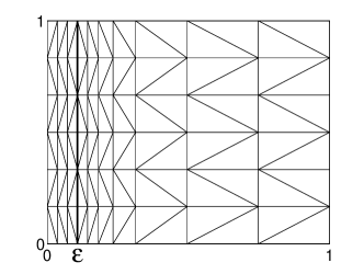
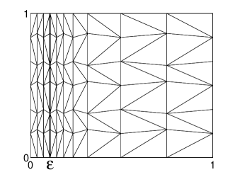
Fig. 10: Non-obtuse triangulation used in §8 (left); its version with obtuse triangles (right).

Our estimator is tested using a simple version of (1.1) with $\Omega=(0,1)^{2}$ and $f=u-F(x,y)$, where $F$ is such that the unique exact solution $u=4y\,(1-y)\,[C_{u}\cos(\pi x/2)-(e^{-x/\varepsilon}-e^{-1/\varepsilon})/(1-e^{-x/\varepsilon})]$ (the latter exhibits a sharp boundary layer at $x=0$); the constant parameter $C_{u}$ in $u$ will take values $1$ and $0$. We consider an a-priori-chosen layer-adapted non-obtuse triangulation, as on Fig. 10 (left), which is obtained by drawing diagonals from the tensor product of the Bakhvalov grid $\{\chi(\frac{i}{N})\}_{i=1}^{N}$ in the $x$-direction [5] and a uniform grid $\{\frac{j}{M}\}_{j=0}^{M}$ in the $y$-direction with $M=\frac{1}{2}N$. The continuous mesh-generating function $\chi(t)=t$ if $\varepsilon>\frac{1}{6}$; otherwise, $\chi(t)=3\varepsilon\ln\frac{1}{1-2t}$ for $t\in(0,\frac{1}{2}-3\varepsilon)$ and is linear elsewhere subject to $\chi(1)=1$. Furthermore, to test our estimator on a mesh with obtuse triangles and, in particular, the role of the estimator components $\boldsymbol{\tau}_{\!S}^{J}$ in (4.3) for $S\in{\mathcal{S}}^{*}$, we distort the initial non-obtuse triangulation by moving some of the nodes upwards/downwards by $\min\{\mathring{h}_{z},\,\frac{1}{8}H_{z}\}$; see Fig. 10 (right).

Table 1: Test problem with $C_{u}=1$, non-obtuse triangulation (see Fig. 10, left).

$N$	$\varepsilon=1$	$\varepsilon=2^{-5}$	$\varepsilon=2^{-10}$	$\varepsilon=2^{-15}$	$\varepsilon=2^{-20}$	$\varepsilon=2^{-25}$	$\varepsilon=2^{-30}$
	Errors $\vvvert u_{h}-u\vvvert_{\varepsilon\,;\Omega}$
64	3.203e-2	5.204e-3	1.065e-3	6.734e-4	6.576e-4	6.571e-4	6.571e-4
128	1.602e-2	2.594e-3	4.534e-4	1.797e-4	1.641e-4	1.636e-4	1.636e-4
256	8.011e-3	1.296e-3	2.157e-4	5.533e-5	4.133e-5	4.081e-5	4.080e-5
512	4.006e-3	6.479e-4	1.062e-4	2.130e-5	1.071e-5	1.020e-5	1.019e-5
	${\mathcal{S}}^{*}=\emptyset$ in (4.3):  Estimators (odd rows)  &  Effectivity Indices (even rows)
64	3.301e-2	6.994e-3	1.325e-3	6.878e-4	6.581e-4	6.572e-4	6.571e-4
	1.031	1.344	1.244	1.021	1.001	1.000	1.000
128	1.647e-2	2.698e-3	6.007e-4	1.928e-4	1.645e-4	1.636e-4	1.636e-4
	1.028	1.040	1.325	1.073	1.003	1.000	1.000
256	8.232e-3	1.335e-3	2.928e-4	6.541e-5	4.178e-5	4.083e-5	4.080e-5
	1.028	1.030	1.357	1.182	1.011	1.000	1.000
512	4.115e-3	6.668e-4	1.460e-4	2.753e-5	1.115e-5	1.022e-5	1.019e-5
	1.027	1.029	1.375	1.292	1.041	1.001	1.000

Table 2: Test problem with $C_{u}=1$, mesh with obtuse triangles (see Fig. 10, right).

$N$	$\varepsilon=1$	$\varepsilon=2^{-5}$	$\varepsilon=2^{-10}$	$\varepsilon=2^{-15}$	$\varepsilon=2^{-20}$	$\varepsilon=2^{-25}$	$\varepsilon=2^{-30}$
	Errors $\vvvert u_{h}-u\vvvert_{\varepsilon\,;\Omega}$
64	3.334e-2	5.311e-3	1.095e-3	7.218e-4	7.072e-4	7.067e-4	7.067e-4
128	1.669e-2	2.647e-3	4.580e-4	1.913e-4	1.768e-4	1.763e-4	1.763e-4
256	8.352e-3	1.323e-3	2.161e-4	5.774e-5	4.451e-5	4.404e-5	4.402e-5
512	4.177e-3	6.612e-4	1.061e-4	2.170e-5	1.149e-5	1.101e-5	1.100e-5
	${\mathcal{S}}^{*}=\emptyset$ in (4.3):  Estimators (odd rows)  &  Effectivity Indices (even rows)
64	3.546e-2	8.155e-3	1.666e-3	7.554e-4	7.083e-4	7.068e-4	7.067e-4
	1.064	1.535	1.521	1.047	1.002	1.000	1.000
128	1.772e-2	3.556e-3	8.999e-4	2.370e-4	1.785e-4	1.764e-4	1.763e-4
	1.062	1.343	1.965	1.239	1.010	1.000	1.000
256	8.866e-3	1.770e-3	5.948e-4	1.254e-4	4.867e-5	4.417e-5	4.403e-5
	1.061	1.339	2.752	2.171	1.093	1.003	1.000
512	4.434e-3	8.842e-4	3.927e-4	1.063e-4	2.169e-5	1.148e-5	1.101e-5
	1.062	1.337	3.703	4.896	1.889	1.043	1.001
	${\mathcal{S}}^{*}\neq\emptyset$ in (4.3):  Estimators (odd rows)  &  Effectivity Indices (even rows)
64	3.546e-2	8.149e-3	1.536e-3	7.466e-4	7.080e-4	7.068e-4	7.067e-4
	1.064	1.534	1.402	1.034	1.001	1.000	1.000
128	1.772e-2	3.553e-3	7.089e-4	2.140e-4	1.776e-4	1.763e-4	1.763e-4
	1.062	1.342	1.548	1.118	1.005	1.000	1.000
256	8.866e-3	1.770e-3	3.474e-4	7.509e-5	4.532e-5	4.406e-5	4.402e-5
	1.061	1.338	1.607	1.300	1.018	1.001	1.000
512	4.434e-3	8.839e-4	1.732e-4	3.238e-5	1.225e-5	1.104e-5	1.100e-5
	1.062	1.337	1.633	1.492	1.066	1.002	1.000

Table 3: Test problem with $C_{u}=0$, mesh with obtuse triangles (see Fig. 10, right).

$N$	$\varepsilon=1$	$\varepsilon=2^{-5}$	$\varepsilon=2^{-10}$	$\varepsilon=2^{-15}$	$\varepsilon=2^{-20}$	$\varepsilon=2^{-25}$	$\varepsilon=2^{-30}$
	Errors $\vvvert u_{h}-u\vvvert_{\varepsilon\,;\Omega}$
64	5.329e-2	4.862e-3	8.425e-4	1.489e-4	2.633e-5	4.655e-6	8.228e-7
128	2.680e-2	2.438e-3	4.222e-4	7.469e-5	1.320e-5	2.334e-6	4.126e-7
256	1.344e-2	1.220e-3	2.110e-4	3.740e-5	6.611e-6	1.169e-6	2.066e-7
512	6.727e-3	6.104e-4	1.051e-4	1.871e-5	3.308e-6	5.848e-7	1.034e-7
	${\mathcal{S}}^{*}=\emptyset$ in (4.3):  Estimators (odd rows)  &  Effectivity Indices (even rows)
64	5.729e-2	7.763e-3	1.487e-3	2.632e-4	4.652e-5	8.224e-6	1.454e-6
	1.075	1.597	1.765	1.767	1.767	1.767	1.767
128	2.881e-2	3.383e-3	8.710e-4	1.565e-4	2.766e-5	4.891e-6	8.645e-7
	1.075	1.388	2.063	2.095	2.095	2.095	2.095
256	1.444e-2	1.689e-3	5.883e-4	1.167e-4	2.063e-5	3.648e-6	6.448e-7
	1.075	1.384	2.788	3.121	3.121	3.121	3.121
512	7.231e-3	8.443e-4	3.903e-4	1.055e-4	1.866e-5	3.299e-6	5.832e-7
	1.075	1.383	3.713	5.638	5.642	5.642	5.642
	${\mathcal{S}}^{*}\neq\emptyset$ in (4.3):  Estimators (odd rows)  &  Effectivity Indices (even rows)
64	5.729e-2	7.668e-3	1.370e-3	2.422e-4	4.282e-5	7.569e-6	1.338e-6
	1.075	1.577	1.626	1.626	1.626	1.626	1.626
128	2.881e-2	3.330e-3	6.870e-4	1.215e-4	2.148e-5	3.797e-6	6.712e-7
	1.075	1.366	1.627	1.627	1.627	1.627	1.627
256	1.444e-2	1.660e-3	3.437e-4	6.086e-5	1.076e-5	1.902e-6	3.362e-7
	1.075	1.360	1.629	1.627	1.627	1.627	1.627
512	7.231e-3	8.301e-4	1.715e-4	3.046e-5	5.385e-6	9.519e-7	1.683e-7
	1.075	1.360	1.632	1.628	1.628	1.628	1.628

In our numerical experiments, we set ${\mathcal{T}}_{0}:=\emptyset$ in (3.3) and replace $\lesssim$ by $\leq$ in (3.3), (4.3), and when dealing with the two cases $h_{z}\lesssim\varepsilon$ and $h_{z}\not\lesssim\varepsilon$, as well as with $h_{T}\lesssim\varepsilon$ in (6.1). Also, we understand $a\ll b$ as $a\leq\frac{1}{5}b$ for any two quantities $a$ and $b$ (so, for example, (3.3) becomes ${\mathcal{T}}^{*}:=\{T\in{\mathcal{T}}:h_{T}\leq\frac{1}{5}H_{T}\mbox{~{}and~{}}h_{T}\leq\varepsilon\}$).

We compute the estimator $\mathcal{E}$ from (4.2) with $C_{f}:=1$ and $\boldsymbol{\tau}$ from (4.3), (4.6). For the non-obtuse mesh of Fig. 10 (left), conditions ${\mathcal{A}}1$ and ${\mathcal{A}}2$ are satisfied, so we set ${\mathcal{S}}^{*}=\emptyset$. The component $\boldsymbol{\tau}_{\!z}$ in (4.3) is computed by (5.1) combined with (5.3) for $h_{z}\leq\varepsilon$, and, otherwise, using (7.3), (7.4), (7.5) combined with (7.6). Note that instead of explicitly including the components involving $\boldsymbol{\tau}_{z;T}^{\pm}$ (from (7.4)) in $\boldsymbol{\tau}$, we use (7.1b) (as well as Remark 18). This somewhat simplifies the computations, but yields a slightly less sharp estimator. Similarly, whenever $\phi_{z}^{*}\neq\phi_{z}$ in (7.4), we employ the bounds from (7.2). When computing the error and the estimator, we replace $\nabla u$ by its linear Lagrange interpolant, and $u$ and $f_{h}$ by their quadratic Lagrange interpolants.

When using the mesh with obtuse triangles of Fig. 10 (right), we consider ${\mathcal{S}}^{*}$ defined by (6.1), and also compare the latter with a simpler choice ${\mathcal{S}}^{*}=\emptyset$. Whenever ${\mathcal{S}}^{*}\neq\emptyset$, the estimator involves $\boldsymbol{\tau}_{\!S}^{J}$ computed by (6.2), while the computation of $\boldsymbol{\tau}_{\!z}$ employs (6.4) and Remark 20.

For the test problem with $C_{u}=1$, the errors $\vvvert u_{h}-u\vvvert_{\varepsilon\,;\Omega}$ are compared with the corresponding estimators $\mathcal{E}$ in Tables 1 and 2. One observes that the effectivity indices (computed as the ratio of the estimator to the error) do not exceed 1.633, as long as ${\mathcal{S}}^{*}\neq\emptyset$ for the mesh with obtuse triangles. By contrast, ${\mathcal{S}}^{*}=\emptyset$ on the mesh with obtuse triangles larger and less stable effectivity indices. But the superiority of the estimator with ${\mathcal{S}}^{*}\neq\emptyset$ is particularly evident for the test problem with $C_{u}=0$ on the mesh with obtuse triangles; compare the effectivity indices for the two choices of ${\mathcal{S}}^{*}$ in Table 3. Some additional numerical results are given in Appendix A.

Overall, for the considered ranges of $\varepsilon$ and $N$, the aspect ratios of the mesh elements take values between 2 and 3.6e+8. Considering these variations, our estimator ${\mathcal{E}}$ performs quite well and its effectivity indices do not exceed 1.63 and stabilize as $\varepsilon\rightarrow 0$ and $N$ increases (as long as ${\mathcal{S}}^{*}\neq\emptyset$ is used for the mesh with obtuse triangles). We have also observed that the inclusion of the estimator components $\boldsymbol{\tau}_{\!S}^{J}$ in (4.3) for $S\in{\mathcal{S}}^{*}\neq\emptyset$, in general, yields a superior estimator. A more comprehensive numerical study of the proposed estimator certainly needs to be conducted, and will be presented elsewhere.

9 Lower error bounds. Estimator efficiency

Throughout this section, we additionally assume that $f(x,y;u)-f(x,y;v)\lesssim|u-v|$, and use the additional notation $J_{S}:=[\partial_{\boldsymbol{\nu}}u_{h}]_{S}$ and $\omega_{S}:=T\cup T^{\prime}$ for any $S=\partial T\cap\partial T^{\prime}\in{\mathcal{S}}$ (with the obvious modification $\omega_{S}:=T$ for the case $S\subset\partial T\cap\partial\Omega$).

Table 4: Lower error estimators for test problem with $u=\sin(\pi ax)$ and $\varepsilon=1$.

		$\,a=1$				$\,a=3$
		$N=20$	$N=40$	$N=80$		$N=20$	$N=40$	$N=80$
		Errors $\vvvert u_{h}-u\vvvert_{\varepsilon\,;\Omega}$ (odd rows)  &  $\|h_{T}(f_{h}-f_{h}^{I})\|_{\Omega}$ (even rows)
$M=\;\;\;2N$		1.01e-1	5.04e-2	2.52e-2		9.26e-1	4.56e-1	2.27e-1
		3.87e-4	4.84e-5	6.05e-6		2.87e-2	3.59e-3	4.50e-4
$M=\;\;\;8N$		1.01e-1	5.04e-2	2.52e-2		9.26e-1	4.56e-1	2.27e-1
		1.07e-4	1.34e-5	1.68e-6		7.95e-3	9.97e-4	1.25e-4
$M=\;32N$		1.01e-1	5.04e-2	2.52e-2		9.26e-1	4.56e-1	2.27e-1
		2.70e-5	3.38e-6	4.22e-7		2.00e-3	2.51e-4	3.14e-5
$M=\!128N$		1.01e-1	5.04e-2	2.52e-2		9.26e-1	4.56e-1	2.27e-1
		6.76e-6	8.45e-7	1.06e-7		5.01e-4	6.28e-5	7.86e-6
		$\underline{\mathcal{E}}$ using $\varrho_{S\rm\scriptsize(\cite[cite]{[\@@bibref{}{Kun01}{}{}]})}$ (odd rows)  &  Effectivity Indices (even rows)
$M=\;\;\;2N$		2.89e-1	1.45e-1	7.24e-2		2.51e+0	1.26e+0	6.33e-1
		2.87	2.88	2.88		2.72	2.78	2.79
$M=\;\;\;8N$		1.32e-1	6.59e-2	3.30e-2		1.17e+0	5.86e-1	2.93e-1
		1.31	1.31	1.31		1.26	1.29	1.29
$M=\;32N$		6.27e-2	3.14e-2	1.57e-2		5.62e-1	2.82e-1	1.41e-1
		0.62	0.62	0.62		0.61	0.62	0.62
$M=\!128N$		3.10e-2	1.55e-2	7.75e-3		2.79e-1	1.39e-1	6.97e-2
		0.31	0.31	0.31		0.30	0.31	0.31
		$\underline{\mathcal{E}}$ using $\varrho_{S\rm(\S\ref{ssec_new_lower})}$ (odd rows)  &  Effectivity Indices (even rows)
$M=\;\;\;2N$		3.00e-1	1.50e-1	7.52e-2		2.61e+0	1.32e+0	6.59e-1
		2.98	2.98	2.98		2.82	2.89	2.90
$M=\;\;\;8N$		2.51e-1	1.26e-1	6.28e-2		2.25e+0	1.13e+0	5.64e-1
		2.49	2.49	2.49		2.43	2.47	2.48
$M=\;32N$		2.47e-1	1.23e-1	6.18e-2		2.21e+0	1.11e+0	5.56e-1
		2.45	2.45	2.45		2.39	2.44	2.45
$M=\!128N$		2.46e-1	1.23e-1	6.17e-2		2.21e+0	1.11e+0	5.55e-1
		2.44	2.45	2.45		2.39	2.43	2.45

9.1 Standard lower error bounds are not sharp. Numerical example

Consider a simple test problem (1.1) with $\varepsilon=1$, the unique exact solution $u=\sin(\pi ax)$ (for $a=1,3$), and $f=u-F(x,y)$ on $\Omega=(0,1)^{2}$. We employ the triangulation obtained by drawing diagonals from the tensor product of the uniform grids $\{\frac{i}{N}\}_{i=0}^{N}$ and $\{\frac{j}{M}\}_{j=0}^{M}$ respectively in the $x$- and $y$-directions (with all diagonals having the same orientation). The standard lumped-mass quadrature, i.e. ${\mathcal{T}}_{*}:=\emptyset$ in (3.2), will be used in numerical experiments in this section (while the anisotropic quadrature with ${\mathcal{T}}_{*}:={\mathcal{T}}$ produces very similar results on this mesh).

For this problem, we compare two lower error estimators: obtained using the standard bubble function approach [19] (see also Lemma 22 in §9.2) and the one obtained in §9.3 (combine Theorem 25 with Lemma 22). They can be described by

$$\underline{\mathcal{E}}:=\Bigl{\{}\sum_{S\in{\mathcal{S}}\backslash\partial\Omega}\varrho_{S}\,J_{S}^{2}+\|h_{T}f_{h}^{I}\|_{\Omega}^{2}\Bigr{\}}^{1/2}\lesssim\vvvert u_{h}-u\vvvert_{\varepsilon\,;\Omega}+\|h_{T}(f_{h}-f_{h}^{I})\|_{\Omega},$$ (9.1a)

where the weight $$\varrho_{S} S\in{\mathcal{S}}\backslash\partial\Omega$$ for is defined by

$$\varrho_{S}=\left\{\begin{array}[]{lll}\varrho_{S\rm\scriptsize(\cite[cite]{[\@@bibref{}{Kun01}{}{}]})}&\!\!\!\!\!\!{}=|S|\displaystyle\min_{T\subset\omega_{S}}\{h_{T}\},&\mbox{\cite[cite]{[\@@bibref{}{Kun01}{}{}]} using bubble functions (also \S\ref{ssec_kun_})},\\[11.38092pt] \varrho_{S\rm(\S\ref{ssec_new_lower})}&\!\!\!\!\!\!{}=\frac{1}{2}|\omega_{S}|,&\mbox{see Theorem~{}\ref{theo_lower} in \S\ref{ssec_new_lower}}.\end{array}\right.$$ (9.1b)

(To be more precise, when $\varrho_{S\rm(\S\ref{ssec_new_lower})}$ is used, the term $\|h_{T}(f_{h}-f_{h}^{I})\|_{\Omega}$ in the right-hand side of (9.1a) should be replaced by a larger $\|H_{T}\,{\rm osc}(f_{h}\,;T)\|_{\Omega}$; see §9.3 for details.)

To address whether the left-hand side $\underline{\mathcal{E}}$ in (9.1a) is sharp, the errors $\vvvert u_{h}-u\vvvert_{\varepsilon\,;\Omega}$ (as well as $\|h_{T}(f_{h}-f_{h}^{I})\|_{\Omega}$) are compared with $\underline{\mathcal{E}}$ in Table 4. Clearly, the standard lower estimator using the weights $\varrho_{S\rm\scriptsize(\cite[cite]{[\@@bibref{}{Kun01}{}{}]})}$ is not sharp. Not only its effectivity indices strongly depend on the ratio $M/N$, but, perhaps more alarmingly, $\underline{\mathcal{E}}$ converges to zero as $M/N$ increases, i.e. the mesh is anisotropically refined in the wrong direction (while the error remains almost independent of $M/N$). By contrast, the estimator of §9.3 performs quite well, with the effectivity indices stabilizing.

When comparing the two estimators, note that $\varrho_{S\rm\scriptsize(\cite[cite]{[\@@bibref{}{Kun01}{}{}]})}\simeq\varrho_{S\rm(\S\ref{ssec_new_lower})}$ when $|S|\simeq{\rm diam}\,\omega_{S}$, however, $\varrho_{S\rm\scriptsize(\cite[cite]{[\@@bibref{}{Kun01}{}{}]})}\ll\varrho_{S\rm(\S\ref{ssec_new_lower})}$ when $|S|\ll{\rm diam}\,\omega_{S}$, i.e. for short edges. Hence, our numerical experiments suggest that it is the short-edge jump residual terms in the standard lower estimator that are not sharp. We shall address this theoretically in §9.3.

9.2 Lower error bounds using the standard bubble approach

Here, for completeness, we prove a version of the lower error bounds from [19, Theorem 4.3] for the semilinear case (similar, but less sharp bounds can also be found in [18, 20]).

Lemma 22.

For a solution $u$ of (1.1) and any $u_{h}\in S_{h}$, one has

$$\min\{1,\,h_{T}\varepsilon^{-1}\}\|f_{h}^{I}\|_{T} \lesssim\underbrace{\vvvert u_{h}-u\vvvert_{\varepsilon\,;{T}}+\min\{1,\,h_{T}\varepsilon^{-1}\}\|f_{h}-f_{h}^{I}\|_{T}}_{{}=:{\mathcal{Y}}_{T}} \forall T\in{\mathcal{T}},$$ (9.2a)

$$|S|^{1/2}\,\,\bigl{|}\varepsilon J_{S}\bigr{|} \lesssim\sum_{T\in\omega_{S}}{\mathcal{Y}}_{T}\,\min\{\varepsilon,\,h_{T}\}^{-1/2} \forall S\in{\mathcal{S}}\backslash\partial\Omega.$$ (9.2b)

Corollary 23.

If $|\omega_{z}|\simeq|T|$ for any $T\subset\omega_{z}$, then

$$\min\{1,\,\varepsilon h_{z}^{-1}\}^{1/2}\,\,\|\varepsilon\widetilde{J}_{z}\|_{\omega_{z}}+\min\{1,\,h_{z}\varepsilon^{-1}\}\|f_{h}^{I}\|_{\omega_{z}}\lesssim\sum_{T\subset\omega_{z}}{\mathcal{Y}}_{T}\,,\vspace{-0.4cm}$$

$$\mbox{where}\qquad\quad\widetilde{J}_{z}:=\underbrace{\max_{S\in\gamma_{z}:|S|\simeq H_{z}}\bigl{|}J_{S}\bigr{|}}_{{}=:\widehat{J}_{z}}\,\,+\,\,\{h_{z}H_{z}^{-1}\}^{1/2}\underbrace{\max_{S\in\gamma_{z}:|S|\ll H_{z}}\bigl{|}J_{S}\bigr{|}}_{{}=:\mathring{J}_{z}}.\hphantom{\mbox{where}\qquad\quad}\vspace{-0.2cm}$$ (9.3)

Remark 24 (Estimator efficiency under an adaptive-mesh-alignment condition).

It appears that the above result is as sharp as one can get using the bubble function approach, while in §9.1 we have seen that the short-edge jump residual terms are not sharp in such bounds. On the other hand, the interpolation error bounds suggest that a reasonably optimal and correctly-aligned mesh may be expected to satisfy $\mathring{J}_{z}\lesssim\widehat{J}_{z}$. Consequently, it appears reasonable to impose a mild version of this condition:

$$\varepsilon\mathring{J}_{z}\lesssim\varepsilon\widehat{J}_{z}+\min\{1,\,\varepsilon h_{z}^{-1}\}^{-1/2}\min\{1,\,h_{z}\varepsilon^{-1}\}\|f_{h}^{I}\|_{L_{\infty}(\omega_{z})}.$$ (9.4)

when constructing a mesh adaptively. Clearly, if both (9.4) and the condition of the above corollary are satisfied for all $z\in\mathcal{N}$, then the upper error estimator from (1.2) is efficient.

Proof of Lemma 22. (i) On any $T\in\mathcal{T}$, consider $w:=f_{h}^{I}\,\phi_{1}\phi_{2}\phi_{3}$, where $\{\phi_{i}\}_{i=1}^{3}$ are the standard hat functions associated with the three vertices of $T$. Now, a standard calculation yields $\|f_{h}^{I}\|_{T}^{2}\simeq\langle f_{h}^{I},w\rangle$. So, using $f_{h}^{I}=-\varepsilon^{2}\triangle u_{h}+f_{h}^{I}$ and (1.1) yields $\|f_{h}^{I}\|_{T}^{2}\simeq\varepsilon^{2}\langle\nabla(u_{h}-u),\nabla w\rangle+\langle f_{h}^{I}-f(\cdot;u),w\rangle$. Next, invoking $\|\nabla w\|_{T}\lesssim h_{T}^{-1}\|w\|_{T}$, one arrives at

$$\|f_{h}^{I}\|_{T}^{2}\lesssim\Bigl{(}(\varepsilon h_{T}^{-1}+1)\vvvert u_{h}-u\vvvert_{\varepsilon\,;{T}}+\|f_{h}-f_{h}^{I}\|_{T}\Bigr{)}\,\|w\|_{T}\,.$$

Here we also used $|f_{h}^{I}-f(\cdot;u)|\lesssim|u_{h}-u|+|f_{h}-f_{h}^{I}|$. The desired result (9.2a) follows in view of $\|w\|_{T}\lesssim\|f_{h}^{I}\|_{T}$ and $\varepsilon h_{T}^{-1}+1\simeq\min\{1,\,h_{T}\varepsilon^{-1}\}^{-1}$.

(ii) For each of the two triangles $T\subset\omega_{S}$, introduce a triangle $\widetilde{T}\subseteq T$ with an edge $S$ such that $|\widetilde{T}|\simeq\min\{\varepsilon,\,h_{T}\}|S|$. Next, set $w:=J_{S}\,\widetilde{\phi}^{\prime}\widetilde{\phi}^{\prime\prime}$, where $\widetilde{\phi}^{\prime}$ and $\widetilde{\phi}^{\prime\prime}$ are the hat functions on the triangulation $\{\widetilde{T}\}_{T\subset\omega_{S}}$ associated with the two end points of $S$ (with $w:=0$ on each $T\backslash\widetilde{T}$ for $T\subset\omega_{S}$). A standard calculation using $\triangle u_{h}=0$ in $T\subset\omega_{S}$ and (1.1), yields

$$|S|\,(\varepsilon J_{S})^{2}\simeq\varepsilon^{2}\int_{S}w\,[\partial_{\boldsymbol{\nu}}u_{h}]_{S}=\varepsilon^{2}\langle\nabla u_{h},\nabla w\rangle=\varepsilon^{2}\langle\nabla(u_{h}-u),\nabla w\rangle-\langle f(\cdot;u),w\rangle.$$

Next, invoking $\|\nabla w\|_{T}\lesssim\min\{\varepsilon,\,h_{T}\}^{-1}\|w\|_{T}$ for any $T\subset\omega_{S}$, we arrive at

$$|S|\,(\varepsilon J_{S})^{2}\lesssim\sum_{T\in\omega_{S}}\underbrace{\Bigl{(}\min\{1,\,h_{T}\varepsilon^{-1}\}^{-1}\vvvert u_{h}-u\vvvert_{\varepsilon\,;T}+\|f_{h}\|_{T}\Bigr{)}}_{{}\lesssim{\mathcal{Y}}_{T}\min\{1,\,h_{T}\varepsilon^{-1}\}^{-1}\;\rm by\;\eqref{lower_f}}\underbrace{\|w\|_{T}}_{\simeq\min\{\varepsilon,\,h_{T}\}^{1/2}|S|^{1/2}|J_{S}|}.\hskip 28.45274pt$$

In view of $\min\{1,\,h_{T}\varepsilon^{-1}\}^{-1}\,\min\{\varepsilon,\,h_{T}\}^{1/2}\,\varepsilon^{-1}\simeq\min\{\varepsilon,\,h_{T}\}^{-1/2}$, one gets (9.2b).

9.3 New lower error bound with sharp short-edge jump residual terms

Throughout this section, we make additional restrictions on the anisotropic mesh as follows. Let $\Omega:=(0,1)^{2}$, and $\{x_{i}\}_{i=0}^{n}$ be an arbitrary mesh in the $x$ direction on the interval $(0,1)$. Then, let each $T\in\mathcal{T}$, for some $i$, (i) have the shortest edge on the line $x=x_{i}$; (ii) have a vertex on the line $x=x_{i+1}$ or $x=x_{i-1}$ (see Fig. 11). Also, let ${\mathcal{N}}={\mathcal{N}}_{\rm ani}$, i.e. each $z\in\mathcal{N}$ be an anisotropic node in the sense of (2.3) and satisfy ${\mathcal{A}}1_{\rm ani}$. The above conditions essentially imply that all mesh elements are anisotropic and aligned in the $x$-direction. The main result of this section is the following.

Fig. 11: Partially structured anisotropic mesh considered in §9.3.

Theorem 25 (Short-edge jump residual terms).

Let $u$ and $u_{h}$ respectively satisfy (1.1) and (3.1), and $\Omega_{i}:=(x_{i-1},x_{i+1})\times(0,1)$. If either no no quadrature is used in $\Omega_{i}$ (i.e. (3.1) involves $\langle f_{h},v_{h}\rangle_{h}=\langle f_{h},v_{h}\rangle$ $\forall v_{h}\in S_{h}$ with support in $\Omega_{i}$), or $\langle\cdot,\cdot\rangle_{h}$ is defined by (3.2)–(3.5) with either $\mathcal{T}\cap\Omega_{i}\subset\mathcal{T}^{*}$, or $\Omega_{i}\cap\mathcal{T}^{*}=\emptyset$, then

$$\sum_{S\in{\mathcal{S}}\cap\{x=x_{i}\}}\!\!\!\min\{\varepsilon|S|,|\omega_{S}|\}\,\bigl{(}\varepsilon{J}_{S}\bigr{)}^{2}\lesssim\underbrace{\vvvert u_{h}-u\vvvert^{2}_{\varepsilon\,;{\Omega_{i}}}+\|\lambda_{T}\,{\rm osc}(f_{h}\,;T)\|^{2}_{\Omega_{i}}}_{{}=\,\sum_{T\subset\Omega_{i}}{\mathcal{Y}}_{T}^{2}\,\,=:\,\,{\mathcal{Y}}_{i}^{2}}\,.$$ (9.5)

To prove this theorem, we shall use an auxiliary result.

Lemma 26.

(i) If $\gamma_{z}\cap\{x=x_{i}\}$ is formed by exactly two edges $S^{-}$ and $S^{+}$, then

$$\bigl{|}J_{{S}^{+}}-J_{{S}^{-}}\bigr{|}\lesssim h_{z}H_{z}^{-1}\!\!\sum_{S\in\gamma_{z}\backslash\{x=x_{i}\}}\!\!\!|J_{S}|.\vspace{-0.1cm}$$ (9.6)

(ii) If $\gamma_{z}\cap\{x=x_{i}\}$ is formed by a single edge $S^{+}\!$, then $J_{{S}^{-}}\!$ in (9.6) is replaced by $0$.

Proof.

(i) Note that in this case $z\not\in\partial\Omega$. Using the notation $\{T_{i}\}$ of §5 (see Fig. 4, centre), let $\llbracket\nabla u_{h}\rrbracket_{\partial T_{i-1}\cap\partial T_{i}}:=\nabla u_{h}\bigr{|}_{\partial T_{i}}-\nabla u_{h}\bigr{|}_{\partial T_{i-1}}$. Then $\sum_{S\in\gamma_{z}}\llbracket\nabla u_{h}\rrbracket_{S}=0$. Multiplying this relation by the unit vector ${\mathbf{i}}_{x}$ in the $x$-direction, and noting that $\llbracket\nabla u_{h}\rrbracket_{{S}^{\pm}}\cdot{\mathbf{i}}_{x}=\pm J_{{S}^{\pm}}$, one gets the desired assertion. We also use the observation that for $S\in\gamma_{z}\backslash\{x=x_{i}\}$, one has $|\llbracket\nabla u_{h}\rrbracket_{S}\cdot{\mathbf{i}}_{x}|\simeq|J_{S}\,{\boldsymbol{\nu}}_{S}\cdot{\mathbf{i}}_{x}|$, where ${\boldsymbol{\nu}}_{S}$ is a unit vector normal to $S$, where, in view of ${\mathcal{A}}1_{\rm ani}$, one has $|{\boldsymbol{\nu}}_{S}\cdot{\mathbf{i}}_{x}|\lesssim h_{z}H_{z}^{-1}$.

(ii) Now $z\in\partial\Omega$, so extend $u_{h}$ to $\mathbb{R}^{2}\backslash\Omega$ by $0$ and imitate the above proof with the modification that now $\sum_{S\in{\mathcal{S}}_{z}}\llbracket\nabla u_{h}\rrbracket_{S}=0$. When dealing with the two edges on $\partial\Omega$, note that for $S\in{\mathcal{S}}_{z}\cap\partial\Omega$, one gets ${\boldsymbol{\nu}}_{S}\cdot{\mathbf{i}}_{x}=0$. ∎

Proof of Theorem 25. Set $H:=x_{i+1}-x_{i-1}$, and $\theta:=\min\bigl{\{}\varepsilon H^{-1},\,\frac{1}{2}\bigr{\}}$, and then $\widetilde{x}_{i\pm 1}:=x_{i}\pm\theta|x_{i\pm 1}-x_{i}|$ and $\widetilde{\Omega}_{i}:=(\widetilde{x}_{i-1},\widetilde{x}_{i+1})\times(0,1)$ (so $\Omega_{i}$ is a rectangular domain, at least, twice as narrow as $\Omega_{i}$). Furthermore, define a triangulation $\widetilde{\mathcal{T}}_{i}$ on $\widetilde{\Omega}_{i}$ by dividing each trapezoid in the partition ${\mathcal{T}}\cap\widetilde{\Omega}_{i}$ into two triangles.

Now, define $v\in C(\bar{\Omega})$ with support in $\widetilde{\Omega}_{i}$ (so $v=0$ on $\partial\widetilde{\Omega}_{i}$) using the standard piecewise-linear interpolation on $\widetilde{\mathcal{T}}_{i}$. Its node values in the interior of $\widetilde{\Omega}_{i}$ are defined by $v(z):={J}_{S}$ for any $z\in\mathcal{N}$ on $\{x=x_{i}\}\backslash\partial\Omega$, where $S\in\gamma_{z}\cap\{x=x_{i}\}$ is any vertical short edge originating at $z$. (For definiteness, let $S$ connect $z$ with the node above it.)

Also, let $v_{h}\in S_{h}$ be the piecewise-linear interpolant of $v$ on the original triangulation ${\mathcal{T}}$ (then $v\in C(\bar{\Omega})$ has support in $\Omega_{i}$), and $w:=v-\theta v_{h}$. Now, a standard calculation yields

$$\underbrace{\varepsilon^{2}\langle\nabla(u_{h}-u),{}\nabla v\rangle+\langle\widehat{f}_{h}-f(\cdot;u),v\rangle}_{{}=:\psi_{1}} {}=\varepsilon^{2}\langle\nabla u_{h},\nabla v\rangle+\langle\widehat{f}_{h},v\rangle\,,$$

$${}=\varepsilon^{2}\langle\partial_{x}u_{h},\partial_{x}w\rangle+\underbrace{\varepsilon^{2}\langle\partial_{y}u_{h},\partial_{y}w\rangle+\langle\widehat{f}_{h},v\rangle-\theta\langle\widehat{f}_{h},v_{h}\rangle_{h}}_{{}=:\psi_{2}}.$$ (9.7)

Here we used a function $\widehat{f}_{h}\approx f_{h}$, which will be specified later subject to the condition $\|\lambda_{T}(\widehat{f}_{h}-f_{h})\|_{\Omega_{i}}\lesssim\|\lambda_{T}\,{\rm osc}(f_{h}\,;T)\|_{\Omega_{i}}\leq{\mathcal{Y}}_{i}$.

With ${\boldsymbol{\nu}}_{x}:=({\boldsymbol{\nu}}\cdot{\mathbf{i}}_{x}){\mathbf{i}}_{x}$ (which is the standard vector projection of the outward normal vector ${\boldsymbol{\nu}}$ onto ${\mathbf{i}}_{x}$), one gets

$$\langle\partial_{x}u_{h},\partial_{x}w\rangle {}=\sum_{S\subset{\mathcal{S}}\cap\Omega_{i}}\int_{S}[\nabla u_{h}\cdot{\boldsymbol{\nu}}_{x}]w=\sum_{S\subset{\mathcal{S}}\cap\{x=x_{i}\}}\int_{S}[\nabla u_{h}\cdot{\boldsymbol{\nu}}_{x}]w,$$

where for $S\subset{\mathcal{S}}\cap\Omega_{i}\backslash\{x=x_{i}\}$, we used $\int_{S}w=\int_{S}v-\theta\int_{S}v_{h}=0$ (as each of $v$ and $v_{h}$ is linear on its support on $S$, and $v=v_{h}$ on $\{x=x_{i}\}$). Next, note that for $S\subset{\mathcal{S}}\cap\{x=x_{i}\}$, one has $|S|\simeq H^{-1}|\omega_{S}|$, while $[\nabla u_{h}\cdot{\boldsymbol{\nu}}_{x}]={J}_{S}$ and $w=(1-\theta)v$ with $v\geq{J}_{S}-{\rm osc}(v\,;S)$ (as $v=J_{S}$ at one of the end points of $S$), so

$$\langle\partial_{x}u_{h},\partial_{x}w\rangle\geq(1-\theta)H^{-1}\!\!\!\sum_{S\subset{\mathcal{S}}\cap\{x=x_{i}\}}\!\!\!|\omega_{S}|\,{J}_{S}\bigl{\{}{J}_{S}-{\rm osc}(v\,;S)\bigr{\}}.$$

Combining the latter with (9.7) multiplied by $\theta H$, and noting that $1-\theta\geq\frac{1}{2}$, one now gets

$$\sum_{S\subset{\mathcal{S}}\cap\{x=x_{i}\}}\!\!\!\theta|\omega_{S}|\,(\varepsilon{J}_{S})^{2}\lesssim\!\!\!\sum_{S\subset{\mathcal{S}}\cap\{x=x_{i}\}}\!\!\!\theta|\omega_{S}|\,\bigl{(}\varepsilon\,{\rm osc}(v\,;S)\bigr{)}^{2}+(\theta H)|\psi_{1}-\psi_{2}|\,.$$ (9.8)

We claim that, to complete the proof, it suffices to get a somewhat similar bound:

$$\sum_{S\subset{\mathcal{S}}\cap\{x=x_{i}\}}\!\!\!\theta|\omega_{S}|\,(\varepsilon{J}_{S})^{2}\lesssim{\mathcal{Y}}_{i}^{2}+\!\!\!\sum_{S\subset{\mathcal{S}}\cap\{x=x_{i}\}}\!\!\!\theta|\omega_{S}|\,\bigl{(}\varepsilon H|S|^{-1}\,{\rm osc}(v\,;S)\bigr{)}^{2}.$$ (9.9)

Indeed, this implies (9.5), as here in the left-hand side, $\theta|\omega_{S}|\simeq\min\{\varepsilon|S|,|\omega_{S}|\}$. Furthermore, using Lemma 26 to estimate ${\rm osc}(v\,;S)$, the sum in the right-hand side of (9.9) is bounded by $\sum_{S\subset{\mathcal{S}}\cap\Omega_{i}\backslash\{x=x_{i}\}}\theta|\omega_{S}|\,(\varepsilon J_{S})^{2}\lesssim\sum_{T\subset\Omega_{i}}{\mathcal{Y}}_{T}^{2}\simeq{\mathcal{Y}}_{i}^{2}$. The latter assertion follows from (9.2b) in view of $\theta|\omega_{S}|\simeq\min\{\varepsilon h_{T},|\omega_{S}|\}\lesssim\min\{\varepsilon|S|,h_{T}|S|\}$ for any $T\subset\omega_{S}$. So it remains to derive (9.9) from (9.8).

For $\psi_{1}$, defined in (9.7), in view of $|f_{h}-f(\cdot;u)|\lesssim|u_{h}-u|$ and $\|\lambda_{T}(\widehat{f}_{h}-f_{h})\|_{\Omega_{i}}\lesssim{\mathcal{Y}}_{i}$, one has

$$|\psi_{1}|\lesssim{\mathcal{Y}}_{i}\,\Bigl{\{}\varepsilon\|\nabla v\|_{\widetilde{\Omega}_{i}}+\|\lambda_{T}^{-1}v\|_{\widetilde{\Omega}_{i}}\Bigr{\}}.$$ (9.10a)

Here, recalling the definition of $$v \partial_{y}v=0 \widetilde{\mathcal{T}}_{i} \{x=x_{i}\} \partial_{y}v=\pm|S|^{-1}{\rm osc}(v\,;S) |\widetilde{T}|\simeq\theta|\omega_{S}| \widetilde{T}\in\widetilde{\mathcal{T}}_{i} S \{x=x_{i}\}$$, note that in any triangle in with a single vertex on , while and for any triangle sharing an edge with , so

$$\|\varepsilon\,\partial_{y}v\|^{2}_{\widetilde{\Omega}_{i}}\lesssim\sum_{S\subset{\mathcal{S}}\cap\{x=x_{i}\}}\!\!\!\theta|\omega_{S}|\,\bigl{(}\varepsilon|S|^{-1}{\rm osc}(v\,;S)\bigr{)}^{2}.$$ (9.10b)

Furthermore, any triangle $$\widetilde{T}\in\widetilde{\mathcal{T}}_{i} S\subset\{x=x_{i}\} |\varepsilon\,\partial_{x}v|\lesssim\varepsilon(\theta H)^{-1}\max_{\widetilde{T}}|v|=\varepsilon(\theta H)^{-1}J_{S} \lambda_{T}^{-1}\simeq\varepsilon(\theta H)^{-1} |\lambda_{T}^{-1}v| |\widetilde{T}|\simeq\theta|\omega_{S}|$$ touches an edge such that , while implies a similar bound for . Combining these observations with yields

$$\|\varepsilon\,\partial_{x}v\|^{2}_{\widetilde{\Omega}_{i}}+\|\lambda_{T}^{-1}v\|^{2}_{\widetilde{\Omega}_{i}}\lesssim\!\!\!\sum_{S\subset{\mathcal{S}}\cap\{x=x_{i}\}}\!\!\!\theta|\omega_{S}|\,\bigl{(}\varepsilon(\theta H)^{-1}J_{S}\bigr{)}^{2}=(\theta H)^{-2}\!\!\!\!\sum_{S\subset{\mathcal{S}}\cap\{x=x_{i}\}}\!\!\!\theta|\omega_{S}|\,(\varepsilon J_{S})^{2}.$$ (9.10c)

To estimate $\psi_{2}$ (defined in (9.7)), set $\widehat{f}_{h}(x,y):=f^{I}_{h}(x_{i},y)$ and $\widehat{v}(x,y):=v(x_{i},y)$ in $\Omega_{i}$. Note that

$$\langle\partial_{y}u_{h},\partial_{y}v\rangle=\theta\,\langle\partial_{y}u_{h},\partial_{y}v_{h}\rangle,\qquad\int_{\widetilde{\Omega}_{i}}\!\widehat{f}_{h}\widehat{v}\,\widetilde{\varphi}_{i}(x)=\theta\,\int_{\Omega_{i}}\!\widehat{f}_{h}\widehat{v}\,\varphi_{i}(x),$$ (9.11)

where $\widetilde{\varphi}_{i}(x)$ and $\varphi_{i}(x)$ are the standard one-dimensional hat functions on the intervals $(\widetilde{x}_{i-1},\widetilde{x}_{i+1})$ and $(x_{i-1},x_{i+1})$, respectively, with $\widetilde{\varphi}_{i}(x_{i})=\varphi_{i}(x_{i})=1$. For the first relation in (9.11), we relied on the observations made on $\partial_{y}v$ when obtaining (9.10b), as well as similar properties of $v_{h}$.

First, consider the case of no quadrature used in $\Omega_{i}$, i.e. $\langle\widehat{f}_{h},v\rangle_{h}=\langle\widehat{f}_{h},v\rangle$. Then

$$\psi_{2}=\int_{\widetilde{\Omega}_{i}}\!\widehat{f}_{h}\bigl{(}v-\widehat{v}\,\widetilde{\varphi}_{i}(x)\bigr{)}-\theta\int_{\Omega_{i}}\!\widehat{f}_{h}\bigl{(}v_{h}-\widehat{v}\,\varphi_{i}(x)\bigr{)}.$$ (9.12)

From this one can show (we shall comment on this below) that

$$|\psi_{2}|\lesssim\underbrace{\bigl{\|}\min\{1,\,h_{T}\varepsilon^{-1}\}\,f_{h}^{I}\bigr{\|}_{\Omega_{i}}}_{{}\lesssim{\mathcal{Y}}_{i}{\rm\;by\;\eqref{lower_f}}}\,\Bigl{\{}\sum_{S\in{\mathcal{S}}\cap\{x=x_{i}\}}\!\!\!\theta|\omega_{S}|\,\bigl{(}\underbrace{\min\{1,\,|S|\varepsilon^{-1}\}^{-1}}_{{}\lesssim\varepsilon|S|^{-1}\theta^{-1}}\,{\rm osc}(v\,;S)\bigr{)}^{2}\Bigr{\}}^{1/2}.$$ (9.13)

Now, combining (9.10) and (9.13) with (9.8) one arrives at the desired assertion (9.9).

To complete the proof, we still need to show that that (9.13) follows from (9.12), as well as $\|\lambda_{T}(\widehat{f}_{h}-f_{h})\|_{\Omega_{i}}\lesssim\|\lambda_{T}\,{\rm osc}(f_{h}\,;T)\|_{\Omega_{i}}$. For each $T\subset\Omega_{i}$, introduce the minimal rectangle $R_{T}=(x_{i-1},x_{i+1})\times(y_{T}^{-},y_{T}^{+})$ containing $T$ (i.e. $(y_{T}^{-},y_{T}^{+})$ is the range of $y$ values within $T$). Note that, crucially, by condition ${\mathcal{A}}1_{\rm ani}$ there is $K\lesssim 1$ such that $|R_{T}|\simeq|T|$ and $R_{T}\subset\omega_{T}^{(K)}\cap\Omega_{i}$, with the notation $\omega_{T}^{(j+1)}$ for the patch of elements in/touching $\omega_{T}^{(j)}$ and $\omega_{T}^{(0)}:=T$. Now, $|v-\widehat{v}\,\widetilde{\varphi}_{i}|\leq{\rm osc}(v\,;R_{T}\cap\{x=x_{i}\})$ for any $T\subset\Omega_{i}$, so (9.12) implies a version of (9.13) with $f_{h}^{I}$ replaced by $\widehat{f}_{h}$, and ${\rm osc}(v\,;S)$ replaced by ${\rm osc}(v\,;R_{T}\cap\{x=x_{i}\})$. As $h_{T^{\prime}}\simeq h_{T}$ and $H_{T^{\prime}}\simeq H_{T}$ for any triangle $T^{\prime}\cap R_{T}\neq\emptyset$, (9.13) follows. Similarly, $|\widehat{f}_{h}-f_{h}|\leq{\rm osc}(f_{h}^{I}\,;R_{T})$ for any $T\subset\Omega_{i}$ implies $\|\lambda_{T}(\widehat{f}_{h}-f_{h})\|_{\Omega_{i}}\lesssim\|\lambda_{T}\,{\rm osc}(f_{h}\,;T)\|_{\Omega_{i}}$.

Finally note that (9.12) is valid only if no quadrature is used in $\Omega_{i}$. Otherwise, the estimation of $\psi_{2}$ needs to be slightly adjusted. For the case ${\mathcal{T}}\cap\Omega_{i}\subset{\mathcal{T}}^{*}$, tweak the definition of $\widehat{f}_{h}$ to $\widehat{f}_{h}(x,y):=\widebar{f}_{i}(y)$, where $\widebar{f}_{i}(y)$ is a one-dimensional piecewise-constant interpolant of $f_{h}$ on $\{x=x_{i}\}\cap\Omega$ such that it is constant on each edge $S\subset\{x=x_{i}\}$. With this modification, $\int_{\Omega_{i}}\!\widehat{f}_{h}\widehat{v}\,\widetilde{\varphi}_{i}(x)=\langle\widehat{f}_{h},v\rangle_{h}$, so the second term in (9.12) vanishes, while all other arguments apply. For the case $\Omega_{i}\cap\mathcal{T}^{*}=\emptyset$, one has $\langle\widehat{f}_{h},v\rangle_{h}=\int_{\Omega}(\widehat{f}_{h},v)^{I}$, so the bound (9.13) on $\psi_{2}$ will additionally include $\|\lambda_{T}\,{\rm osc}(f_{h}^{I}\,;T)\|_{\Omega_{i}}\|\lambda_{T}^{-1}\,v\|_{\widetilde{\Omega}_{i}}$, so (9.10c) is employed again for this additional term.

Remark 27.

Combing the lower error bounds (9.2) and (9.5) and comparing the resulting lower bound with the upper error bound (1.2), one concludes that for the estimator to be efficient, the term $\min\{1,\,\varepsilon h_{z}^{-1}\}\|\varepsilon J_{z}\|^{2}_{\omega_{z}}$ should be replaced by $\sum_{S\in\gamma_{z}}\min\{\varepsilon|S|,|\omega_{z}|\}\,(\varepsilon{J}_{S})^{2}$ in (1.2), and, equivalently, in (4.8). When $h_{z}\gtrsim\varepsilon$, this improvement follows from the first relation in (7.7). Otherwise, if $H_{z}\lesssim\varepsilon$, this follows from $|\omega_{z}|\lesssim\varepsilon|S|$. For the remaining case $h_{z}\lesssim\varepsilon\lesssim H_{z}$, assuming $z\in{\mathcal{N}}_{\rm ani}$ under condition ${\mathcal{A}}1_{\rm ani}$, this sharper upper bound can be shown for a slightly more intricate version of $\boldsymbol{\tau}_{\!z}$, defined as follows. Using the notation of (5.1a) and (7.1) (see Fig. 4 and Fig. 6 (left); also assume that $\boldsymbol{\tau}_{z;T}^{\pm}\in L_{2}(\Omega)$ has support on $T$), set

$$\boldsymbol{\tau}_{\!z}:=\sum_{i=1,m_{z}}{\textstyle\frac{1}{2}}J_{S_{i}^{-}}\bigl{(}\boldsymbol{\tau}_{z;T_{i-1}}^{+}+\boldsymbol{\tau}_{z;T_{i}}^{-}\bigr{)}+\phi_{z}\sum_{i=1}^{N_{z}}\bigl{(}\alpha_{i}{\boldsymbol{\nu}}_{i}+\beta_{i}d_{i}^{-1}\boldsymbol{\mu}_{i}\bigr{)}\,\mathbbm{1}_{(x,y)\in T_{i}}\,,$$

where $\{\alpha_{i}\}$ and $\{\beta_{i}\}$ are chosen to minimize (5.4) subject to the constraints (5.1c), in which $\bigl{[}\partial_{\boldsymbol{\nu}}u_{h}\bigr{]}_{\partial T_{i-1}\cap\partial T_{i}}$ for $i=1,m_{z}$ are replaced by $0$; see Appendix B.

It appears, however, that in most practical situations, this modification of $\boldsymbol{\tau}_{\!z}$ will not improve the estimator, as the short-edge jump residual terms in the upper error estimator are expected to be dominated by the other terms (as discussed in Remark 24).

Appendix A Additional numerical results

We again consider the test problem and the meshes from §8, but now look at two components of the the error in the energy norm. It is reasonable to assume that

$$\vvvert u_{h}-u\vvvert_{\varepsilon\,;\Omega}\simeq\bigl{\{}\varepsilon^{2}\|\nabla u_{h}-(\nabla u)^{I}\|^{2}_{\Omega}+\|u_{h}-u^{I}\|^{2}_{\Omega}\bigr{\}}^{1/2}+\|u-u^{I}\|_{\Omega}\,.$$ (A.1)

Table 5: Test problem with $C_{u}=1$, non-obtuse triangulation (see Fig. 10, left): error component $\bigl{\{}\varepsilon^{2}\|\nabla u_{h}-(\nabla u)^{I}\|^{2}_{2\,;\Omega}+\|u_{h}-u^{I}\|^{2}_{2\,;\Omega}\bigr{\}}^{1/2}$ from (A.1) compared with ${\mathcal{E}}\bigr{|}_{f_{h}:=f_{h}^{I}}$ .

$N$	$\varepsilon=1$	$\varepsilon=2^{-5}$	$\varepsilon=2^{-10}$	$\varepsilon=2^{-15}$	$\varepsilon=2^{-20}$	$\varepsilon=2^{-25}$	$\varepsilon=2^{-30}$
	Errors (odd rows)  &  Computational Rates (even rows)
64	3.203e-2	5.172e-3	8.450e-4	1.489e-4	2.632e-5	4.653e-6	8.225e-7
	1.000	0.997	0.996	0.996	0.996	0.996	0.996
128	1.602e-2	2.591e-3	4.237e-4	7.469e-5	1.320e-5	2.334e-6	4.126e-7
	1.000	0.999	0.999	0.998	0.998	0.998	0.998
256	8.011e-3	1.296e-3	2.119e-4	3.740e-5	6.611e-6	1.169e-6	2.066e-7
	1.000	1.000	1.003	0.999	0.999	0.999	0.999
512	4.006e-3	6.478e-4	1.057e-4	1.871e-5	3.308e-6	5.848e-7	1.034e-7
	${\mathcal{S}}^{*}=\emptyset$ in (4.3):  Estimators (odd rows)  &  Effectivity Indices (even rows)
64	3.290e-2	6.984e-3	1.159e-3	2.047e-4	3.618e-5	6.396e-6	1.131e-6
	1.027	1.350	1.372	1.374	1.375	1.375	1.375
128	1.646e-2	2.695e-3	5.802e-4	1.023e-4	1.808e-5	3.196e-6	5.651e-7
	1.027	1.040	1.369	1.370	1.370	1.370	1.370
256	8.230e-3	1.335e-3	2.908e-4	5.115e-5	9.042e-6	1.598e-6	2.826e-7
	1.027	1.030	1.372	1.368	1.368	1.368	1.368
512	4.115e-3	6.667e-4	1.460e-4	2.558e-5	4.522e-6	7.993e-7	1.413e-7
	1.027	1.029	1.382	1.367	1.367	1.367	1.367

Table 6: Test problem with $C_{u}=1$, non-obtuse triangulation (see Fig. 10, left): error component $\|u-u^{I}\|_{\Omega}$ from (A.1) compared with the estimator component $\|f_{h}-f_{h}^{I}\|_{\Omega}$ .

$N$	$\varepsilon=1$	$\varepsilon=2^{-5}$	$\varepsilon=2^{-10}$	$\varepsilon=2^{-15}$	$\varepsilon=2^{-20}$	$\varepsilon=2^{-25}$	$\varepsilon=2^{-30}$
	Errors (odd rows)  &  Computational Rates (even rows)
64	2.242e-4	6.120e-4	6.496e-4	6.567e-4	6.571e-4	6.571e-4	6.571e-4
	2.000	2.004	2.006	2.006	2.006	2.006	2.006
128	5.607e-5	1.525e-4	1.617e-4	1.635e-4	1.636e-4	1.636e-4	1.636e-4
	2.000	2.002	2.003	2.003	2.003	2.003	2.003
256	1.402e-5	3.807e-5	4.036e-5	4.077e-5	4.079e-5	4.080e-5	4.080e-5
	2.000	2.001	2.002	2.002	2.002	2.002	2.002
512	3.505e-6	9.510e-6	1.008e-5	1.018e-5	1.019e-5	1.019e-5	1.019e-5
	${\mathcal{S}}^{*}=\emptyset$ in (4.3):  Estimators (odd rows)  &  Effectivity Indices (even rows)
64	2.661e-3	5.762e-4	6.484e-4	6.567e-4	6.571e-4	6.571e-4	6.571e-4
	11.867	0.941	0.998	1.000	1.000	1.000	1.000
128	6.671e-4	1.435e-4	1.614e-4	1.634e-4	1.636e-4	1.636e-4	1.636e-4
	11.897	0.941	0.998	1.000	1.000	1.000	1.000
256	1.670e-4	3.579e-5	4.029e-5	4.077e-5	4.079e-5	4.080e-5	4.080e-5
	11.913	0.940	0.998	1.000	1.000	1.000	1.000
512	4.178e-5	8.938e-6	1.006e-5	1.018e-5	1.019e-5	1.019e-5	1.019e-5
	11.921	0.940	0.998	1.000	1.000	1.000	1.000

This error decomposition is useful as the two error components in (A.1) exhibit somewhat different behaviour in our experiments, as${}\simeq\varepsilon^{1/2}N^{-1}$ and${}\simeq N^{-2}$, respectively (compare, for example, the upper parts of Tables  5 and  6). Furthermore, one can identify that ${\mathcal{E}}\bigr{|}_{f_{h}:=f_{h}^{I}}$ (obtained from (4.2) by replacing $f_{h}$ with its linear interpolant $f_{h}^{I}$) essentially estimates the first error component in (A.1) (see Table 5), while $\|f_{h}-f_{h}^{I}\|_{\Omega}$ provides a reasonable estimator for the remaining error component in (A.1) (see Table 6). Indeed, for the estimator components in Tables  5 and  6 (for the latter, when $\varepsilon\leq 2^{-5}$) on the non-obtuse mesh, the effectivity indices do not exceed 1.382 (related results are given in Table 1). For the mesh with obtuse triangles, analogous results are presented in Tables  7 and  8 (with related results in Table  2).

Table 7: Test problem with $C_{u}=1$, mesh with obtuse triangles (see Fig. 10, right): error component $\bigl{\{}\varepsilon^{2}\|\nabla u_{h}-(\nabla u)^{I}\|^{2}_{2\,;\Omega}+\|u_{h}-u^{I}\|^{2}_{2\,;\Omega}\bigr{\}}^{1/2}$ from (A.1) compared with ${\mathcal{E}}\bigr{|}_{f_{h}:=f_{h}^{I}}$ .

$N$	$\varepsilon=1$	$\varepsilon=2^{-5}$	$\varepsilon=2^{-10}$	$\varepsilon=2^{-15}$	$\varepsilon=2^{-20}$	$\varepsilon=2^{-25}$	$\varepsilon=2^{-30}$
	Errors (odd rows)  &  Computational Rates (even rows)
64	3.334e-2	5.274e-3	8.452e-4	1.489e-4	2.632e-5	4.653e-6	8.225e-7
	0.998	0.997	0.996	0.996	0.996	0.996	0.996
128	1.669e-2	2.642e-3	4.236e-4	7.469e-5	1.320e-5	2.334e-6	4.126e-7
	0.999	0.999	1.001	0.998	0.998	0.998	0.998
256	8.352e-3	1.322e-3	2.117e-4	3.740e-5	6.611e-6	1.169e-6	2.066e-7
	1.000	1.000	1.005	0.999	0.999	0.999	0.999
512	4.177e-3	6.611e-4	1.055e-4	1.871e-5	3.308e-6	5.848e-7	1.034e-7
	${\mathcal{S}}^{*}=\emptyset$ in (4.3):  Estimators (odd rows)  &  Effectivity Indices (even rows)
64	3.534e-2	8.142e-3	1.516e-3	2.681e-4	4.739e-5	8.378e-6	1.481e-6
	1.060	1.544	1.794	1.800	1.801	1.801	1.801
128	1.771e-2	3.552e-3	8.840e-4	1.586e-4	2.803e-5	4.955e-6	8.759e-7
	1.061	1.344	2.087	2.123	2.123	2.123	2.123
256	8.864e-3	1.770e-3	5.936e-4	1.174e-4	2.076e-5	3.670e-6	6.487e-7
	1.061	1.339	2.804	3.139	3.140	3.140	3.140
512	4.434e-3	8.842e-4	3.927e-4	1.057e-4	1.870e-5	3.305e-6	5.843e-7
	1.061	1.337	3.722	5.648	5.652	5.652	5.652
	${\mathcal{S}}^{*}\neq\emptyset$ in (4.3):  Estimators (odd rows)  &  Effectivity Indices (even rows)
64	3.534e-2	8.137e-3	1.372e-3	2.422e-4	4.282e-5	7.569e-6	1.338e-6
	1.060	1.543	1.623	1.627	1.627	1.627	1.627
128	1.771e-2	3.550e-3	6.886e-4	1.215e-4	2.148e-5	3.797e-6	6.712e-7
	1.061	1.343	1.626	1.627	1.627	1.627	1.627
256	8.864e-3	1.769e-3	3.453e-4	6.086e-5	1.076e-5	1.902e-6	3.362e-7
	1.061	1.338	1.631	1.627	1.627	1.627	1.627
512	4.434e-3	8.839e-4	1.732e-4	3.046e-5	5.385e-6	9.519e-7	1.683e-7
	1.061	1.337	1.641	1.628	1.628	1.628	1.628

Table 8: Test problem with $C_{u}=1$, mesh with obtuse triangles (see Fig. 10, right): error component $\|u-u^{I}\|_{\Omega}$ from (A.1) compared with the estimator component $\|f_{h}-f_{h}^{I}\|_{\Omega}$ .

$N$	$\varepsilon=1$	$\varepsilon=2^{-5}$	$\varepsilon=2^{-10}$	$\varepsilon=2^{-15}$	$\varepsilon=2^{-20}$	$\varepsilon=2^{-25}$	$\varepsilon=2^{-30}$
	Errors (odd rows)  &  Computational Rates (even rows)
64	2.412e-4	6.591e-4	6.978e-4	7.063e-4	7.067e-4	7.067e-4	7.067e-4
	1.998	2.001	2.001	2.003	2.003	2.003	2.003
128	6.040e-5	1.646e-4	1.743e-4	1.762e-4	1.763e-4	1.763e-4	1.763e-4
	1.999	2.001	2.001	2.002	2.002	2.002	2.002
256	1.511e-5	4.113e-5	4.354e-5	4.399e-5	4.402e-5	4.402e-5	4.402e-5
	1.999	2.000	2.001	2.001	2.001	2.001	2.001
512	3.779e-6	1.028e-5	1.088e-5	1.099e-5	1.100e-5	1.100e-5	1.100e-5
	${\mathcal{S}}^{*}=\emptyset$ in (4.3):  Estimators (odd rows)  &  Effectivity Indices (even rows)
64	2.878e-3	6.274e-4	6.967e-4	7.062e-4	7.067e-4	7.067e-4	7.067e-4
	11.931	0.952	0.998	1.000	1.000	1.000	1.000
128	7.223e-4	1.566e-4	1.740e-4	1.762e-4	1.763e-4	1.763e-4	1.763e-4
	11.958	0.951	0.998	1.000	1.000	1.000	1.000
256	1.809e-4	3.912e-5	4.347e-5	4.399e-5	4.402e-5	4.402e-5	4.402e-5
	11.972	0.951	0.998	1.000	1.000	1.000	1.000
512	4.528e-5	9.777e-6	1.086e-5	1.099e-5	1.100e-5	1.100e-5	1.100e-5
	11.979	0.951	0.998	1.000	1.000	1.000	1.000
	${\mathcal{S}}^{*}\neq\emptyset$ in (4.3): Estimators (odd rows)  &  Effectivity Indices (even rows)
64	2.878e-3	6.274e-4	6.967e-4	7.062e-4	7.067e-4	7.067e-4	7.067e-4
	11.931	0.952	0.998	1.000	1.000	1.000	1.000
128	7.223e-4	1.566e-4	1.740e-4	1.762e-4	1.763e-4	1.763e-4	1.763e-4
	11.958	0.951	0.998	1.000	1.000	1.000	1.000
256	1.809e-4	3.912e-5	4.347e-5	4.399e-5	4.402e-5	4.402e-5	4.402e-5
	11.972	0.951	0.998	1.000	1.000	1.000	1.000
512	4.528e-5	9.777e-6	1.086e-5	1.099e-5	1.100e-5	1.100e-5	1.100e-5
	11.979	0.951	0.998	1.000	1.000	1.000	1.000

Appendix B Justification of Remark 27

To get a sharper version of the upper bound (1.2) for our estimator, with $\min\{1,\,\varepsilon h_{z}^{-1}\}\|\varepsilon J_{z}\|^{2}_{\omega_{z}}$ replaced by a sharper term $\sum_{S\in\gamma_{z}}\min\{\varepsilon|S|,|\omega_{z}|\}\,(\varepsilon{J}_{S})^{2}$, we need to tweak the definition of $\boldsymbol{\tau}_{\!z}$ in (5.1). To be more precise, whenever $h_{z}\lesssim\varepsilon\lesssim H_{z}$ and $\mathring{h}_{z}\not\simeq H_{z}$, let

$$\boldsymbol{\tau}_{\!z} :=\boldsymbol{\tau}_{\!z}^{\prime}+\left\{\begin{array}[]{cl}\displaystyle\sum_{i=1,m}{\textstyle\frac{1}{2}}J_{S_{i}^{-}}\bigl{(}\boldsymbol{\tau}_{z;T_{i-1}}^{+}+\boldsymbol{\tau}_{z;T_{i}}^{-}\bigr{)}&\mbox{if~{}}z\in{\mathcal{N}}_{\rm ani}\backslash{\partial\Omega},\\[14.22636pt] \displaystyle{\textstyle\frac{1}{2}}\mathring{h}_{z}\mathring{\mathcal{J}}_{z}\,\bigl{(}|S_{1}^{+}|^{-1}\boldsymbol{\tau}_{z;T_{1}}^{+}+|S_{n}^{-}|^{-1}\boldsymbol{\tau}_{z;T_{n}}^{-}\bigr{)}&\mbox{if~{}$z$~{}satisfies~{}}{\mathcal{A}}1_{\rm mix},\end{array}\right.$$ (B.1c)

$$\boldsymbol{\tau}_{\!z}^{\prime} :=\phi_{z}\bigl{(}\alpha_{i}{\boldsymbol{\nu}}_{i}+\beta_{i}d_{i}^{-1}\boldsymbol{\mu}_{i}\bigr{)}\quad\forall\ T_{i}\subset\omega_{z},\qquad\qquad\quad\mathring{\mathcal{J}}_{z}:=\mathring{h}_{z}^{-1}\sum_{i=2}^{n}|S_{i}^{-}|J_{S_{i}^{-}}\,.$$ (B.1d)

Here we use the notation of (5.1a) and (7.1) (see Fig. 4 and Fig. 6 (left)), assuming that $\boldsymbol{\tau}_{z;T}^{\pm}\in L_{2}(\Omega)$ has support on $T$, while $m=m_{z}$, $n=n_{z}$ are defined in the proof of Lemma 12. If $z\in{\mathcal{N}}^{*}_{\partial\Omega}$, or $z\in\partial\Omega$ satisfies ${\mathcal{A}}1_{\rm mix}$ and $n_{z}=1$, the definition (5.1) of $\boldsymbol{\tau}_{\!z}$ remains unchanged.

Lemma 28.

Let $\boldsymbol{\tau}_{\!z}$ be modified to (B.1) whenever $h_{z}\lesssim\varepsilon\lesssim H_{z}$ and $\mathring{h}_{z}\not\simeq H_{z}$. Set $\{\alpha_{i},\beta_{i}\}_{i=1}^{N_{z}}$ in (B.1) to minimize (5.4) subject to the constraint $[\boldsymbol{\tau}_{\!z}\cdot{\boldsymbol{\nu}}]=\phi_{z}[\partial_{\boldsymbol{\nu}}u_{h}]$ on $\gamma_{z}$. Then Theorem 5(i) is valid with the term $\min\{1,\,\varepsilon h_{z}^{-1}\}^{1/2}\|\varepsilon J_{z}\|_{\omega_{z}}$ in (4.8) replaced by a sharper $\bigl{\{}\sum_{S\in\gamma_{z}}\min\{\varepsilon|S|,|\omega_{z}|\}\,(\varepsilon{J}_{S})^{2}\bigr{\}}^{1/2}$.

Proof.

For the case $h_{z}\gtrsim\varepsilon$, the sharper version of (4.8) follows from the first relation in (7.7). Otherwise, if $h_{z}\leq H_{z}\lesssim\varepsilon$, this follows from $|\omega_{z}|\lesssim\varepsilon|S|$.

For the remaining case $h_{z}\lesssim\varepsilon\lesssim H_{z}$, using the notation $\mathring{J}_{z}$ and $\widehat{J}_{z}$ of (9.3), we need to show (4.8) with $\min\{1,\,\varepsilon h_{z}^{-1}\}^{1/2}\|\varepsilon J_{z}\|_{\omega_{z}}$ replaced by $\{\varepsilon\mathring{h}_{z}\}^{1/2}\,\varepsilon\mathring{J}_{z}+\|\varepsilon\widehat{J}_{z}\|_{\omega_{z}}$. For $\boldsymbol{\tau}_{\!z}-\boldsymbol{\tau}_{\!z}^{\prime}$, we employ Lemma 17; in particular, (7.1b) implies $\|\varepsilon^{2}{\rm div}(\boldsymbol{\tau}_{\!z}-\boldsymbol{\tau}_{\!z}^{\prime})\|^{2}_{\omega_{z}}\simeq\|\varepsilon(\boldsymbol{\tau}_{\!z}-\boldsymbol{\tau}_{\!z}^{\prime})\|^{2}_{\omega_{z}}\simeq\varepsilon\mathring{h}_{z}(\varepsilon\mathring{J}_{z})^{2}$. Recalling that $g_{z}=\varepsilon^{2}{\rm div}\boldsymbol{\tau}_{\!z}+\theta_{T;z}F_{T;z}$ for $h_{z}\lesssim\varepsilon$, it suffices to prove the desired version of (4.8) for $\|\varepsilon\boldsymbol{\tau}_{\!z}^{\prime}\|_{\omega_{z}}+\|\varepsilon^{2}{\rm div}\boldsymbol{\tau}_{\!z}^{\prime}+\theta_{T;z}F_{T;z}\|_{\omega_{z}}$. In fact, it suffices for the latter to be established for one specific set $\{\alpha_{i},\beta_{i}\}_{i=1}^{N_{z}}$ subject to $[\boldsymbol{\tau}_{\!z}\cdot{\boldsymbol{\nu}}]=\phi_{z}[\partial_{\boldsymbol{\nu}}u_{h}]$ on $\gamma_{z}$. Here the constraint is equivalent to a version of (5.1c) taking into account the possibly non-trivial jumps $[(\boldsymbol{\tau}_{\!z}-\boldsymbol{\tau}_{\!z}^{\prime})\cdot{\boldsymbol{\nu}}]$ across $\gamma_{z}$.

As in the proof of Lemma 12, consider three cases (a), (b) and (c).

(a) Suppose that $z$ satisfies ${\mathcal{A}}1_{\rm mix}$ with $n_{z}\geq 2$. Now, let

$$\alpha_{i}:=\varepsilon^{-2}d_{i}\theta_{T_{i};z}(\widetilde{F}_{T_{i};z}-A_{z})\quad:\quad A_{z}\sum_{i=1}^{N}2\varepsilon^{-2}\theta_{T_{i};z}|T_{i}|:=-\mathring{h}_{z}\mathring{\mathcal{J}}_{z}.$$ (B.2)

Now, the constraint $[\boldsymbol{\tau}_{\!z}\cdot{\boldsymbol{\nu}}]=\phi_{z}[\partial_{\boldsymbol{\nu}}u_{h}]$ on $\gamma_{z}$ yields a version of (5.1c), in which $\frac{1}{2}\mathring{h}_{z}\mathring{\mathcal{J}}_{z}(\mathbbm{1}_{i=2}+\mathbbm{1}_{i=n})$ is subtracted from the right-hand side. Note that the described version of (5.1c) gives a consistent system for $\{\beta_{i}\}_{i=1}^{N}$ with infinitely many solutions, which is shown as in the proof of Lemma 7. In particular, if $z\not\in\partial\Omega$, the consistency of this system can be shown by adding all $N$ equations in this system (and also using ${\boldsymbol{\nu}}_{i}\cdot\bigl{(}|S_{i}^{+}|{\boldsymbol{\nu}}^{+}_{i}+|S_{i}^{-}|{\boldsymbol{\nu}}^{-}_{i}\bigr{)}+2|T_{i}|d_{i}^{-1}=0$), which yields the second relation in (B.2). Note that the latter uniquely defines $A_{z}$ and implies $|A_{z}|\lesssim\varepsilon^{2}|\omega_{z}|^{-1}\mathring{h}_{z}\mathring{J}_{z}$.

Next, set $\beta_{1}:=0$, and imitate the proof of Lemma 12. Now an application of $\sum_{i=2}^{n}$ to the current version of (5.1c) yields $|\beta_{n}d_{n}^{-1}|\simeq|\beta_{n}\mathring{h}_{z}^{-1}|\lesssim\max_{j=1,\ldots,n}|\alpha_{j}|$. Consequently, a version of (5.7) implies $|\beta_{i}d_{i}^{-1}|\lesssim\mathring{J}_{z}+\max_{j=1,\ldots,i}|\alpha_{j}|$ for $i=2,\ldots,n-1$, and $|\beta_{i}d_{i}^{-1}|\lesssim\widehat{J}_{z}+\max_{j=1,\ldots,i}|\alpha_{j}|$ for $i=n+1,\ldots,N$. Note that for $i=2,\ldots,n-1$, one has $|T_{i}|\simeq\mathring{h}_{z}^{2}\lesssim\varepsilon\mathring{h}_{z}$ so $\|\varepsilon\mathring{J}_{z}\|_{T_{i}}\lesssim\{\varepsilon\mathring{h}_{z}\}^{1/2}\,\varepsilon\mathring{J}_{z}$. Note also that $\|\varepsilon\widehat{J}_{z}\|_{T_{i}}\leq\|\varepsilon\widehat{J}_{z}\|_{\omega_{z}}$ for $i=n+1,\ldots,N$. Comparing these observations with the desired version of (4.8) implies that to bound $\|\varepsilon\boldsymbol{\tau}_{\!z}^{\prime}\|_{\omega_{z}}$, it remains to estimate $\max_{i=1,\ldots,N}\|\varepsilon\alpha_{i}\|_{\omega_{z}}$.

For the latter, recall that it was shown in the proof of Lemma 7 that if one sets $A_{z}:=0$ in the current definition of $\alpha_{i}$, then $\max\|\varepsilon\alpha_{i}\|_{\omega_{z}}\lesssim\|h_{z}\varepsilon^{-1}f_{h}^{I}\|_{\omega_{z}}$. For the remaining component $\varepsilon^{-2}d_{i}\theta_{T_{i};z}A_{z}$ of $\alpha_{i}$, recall that $d_{i}\theta_{T_{i};z}\simeq h_{T_{i}}\lesssim h_{z}\lesssim\varepsilon$, so $\varepsilon|\varepsilon^{-2}d_{i}\theta_{T_{i};z}A_{z}|\lesssim|A_{z}|$. On the other hand, $|\varepsilon^{2}{\rm div}\boldsymbol{\tau}_{\!z}^{\prime}+\theta_{T;z}F_{T;z}|\leq|A_{z}|$ (it is a current version of (5.2a)). Hence, to complete the estimation of $\|\varepsilon\boldsymbol{\tau}_{\!z}^{\prime}\|_{\omega_{z}}$, as well as to bound $\|\varepsilon^{2}{\rm div}\boldsymbol{\tau}_{\!z}^{\prime}+\theta_{T;z}F_{T;z}\|_{\omega_{z}}$, we proceed to the bound $\|A_{z}\|_{\omega_{z}}\lesssim|\omega_{z}|^{1/2}(\varepsilon^{2}|\omega_{z}|^{-1}\mathring{h}_{z}\mathring{J}_{z})\lesssim\{\varepsilon\mathring{h}_{z}\}^{1/2}\varepsilon\mathring{J}_{z}$ (in view of $\{\varepsilon\mathring{h}_{z}\}^{1/2}\lesssim|\omega_{z}|^{1/2}$). This observation completes the proof of the desired version of (4.8) in case (a).

(b) Next, consider $z\in{\mathcal{N}}_{\rm ani}\backslash\partial\Omega$ that satisfies ${\mathcal{A}}1_{\rm ani}$ (and so not ${\mathcal{A}}1_{\rm mix}$). Let

$$\alpha_{i}:=\varepsilon^{-2}d_{i}\theta_{T_{i};z}(\widetilde{F}_{T_{i};z}-a_{i})\quad:\quad\sum_{i=1}^{N}2\varepsilon^{-2}\theta_{T_{i};z}|T_{i}|a_{i}=-\sum_{i=1,m}|S_{i}^{-}|J_{S_{i}^{-}}\,.$$ (B.3)

Now, the constraint $[\boldsymbol{\tau}_{\!z}\cdot{\boldsymbol{\nu}}]=\phi_{z}[\partial_{\boldsymbol{\nu}}u_{h}]$ on $\gamma_{z}$ yields a version of (5.1c), in which $\mathbbm{1}_{i\in\{1,m\}}|S_{i}^{-}|J_{S_{i}^{-}}$ is subtracted from the right-hand side. Note that the described version of (5.1c) gives a consistent system for $\{\beta_{i}\}_{i=1}^{N}$ with infinitely many solutions, which is shown as in the proof of Lemma 7. To be more precise, adding all $N$ equations in this system (and also using ${\boldsymbol{\nu}}_{i}\cdot\bigl{(}|S_{i}^{+}|{\boldsymbol{\nu}}^{+}_{i}+|S_{i}^{-}|{\boldsymbol{\nu}}^{-}_{i}\bigr{)}+2|T_{i}|d_{i}^{-1}=0$) yields the second relation in (B.3).

Set

$$a_{i}:=\left\{\begin{array}[]{cl}A_{z}^{+}&\mbox{for}\;\;i=1,\ldots,m,\\ A_{z}^{-}&\mbox{for}\;\;i=m+1,\ldots,N,\end{array}\right.\qquad A_{z}^{+}\sum_{i=1}^{m}2\varepsilon^{-2}\theta_{T_{i};z}|T_{i}|:=\widetilde{\sigma}_{z}\,,$$

where $\widetilde{\sigma}_{z}$ is from (5.8), while $A_{z}^{-}$ is now uniquely defined by the second relation in (B.3). Then, $|A_{z}^{+}|\lesssim\varepsilon H_{z}^{-1}|\varepsilon h_{z}^{-1}\widetilde{\sigma}_{z}|$ and $|A_{z}^{-}|\lesssim|A_{z}^{+}|+\varepsilon H_{z}^{-1}|\varepsilon{J}_{z}|$. Combining these two observations with (5.11) (which was obtained under assumption ${\mathcal{A}}1_{\rm ani}$), one gets

$$A_{z}:=\max_{i=1,\ldots,N}|a_{i}|\lesssim\varepsilon H_{z}^{-1}|\varepsilon J_{z}|+h_{z}\varepsilon^{-1}|\widebar{F}_{z}|+\sum_{T\subset\omega_{z}}\lambda_{T}\,{\rm osc}(f_{h}^{I};T)$$ (B.4)

(where we also used $\varepsilon H_{z}^{-1}\lesssim 1$ for the final two terms).

With these definitions, one gets a version of Lemma 7:

$$|\varepsilon^{2}{\rm div}\boldsymbol{\tau}_{\!z}^{\prime}+\theta_{T;z}\widetilde{F}_{T;z}| \leq A_{z}\qquad\forall\ T\subset\omega_{z},$$ (B.5a)

$$\|\varepsilon\boldsymbol{\tau}_{\!z}^{\prime}\|_{\omega_{z}} \lesssim\|h_{z}\varepsilon^{-1}(|f^{I}_{h}|+A_{z})\|_{\omega_{z}}+\varepsilon\,\Bigl{\{}\sum_{i=1}^{N_{z}}\beta^{2}_{i}d_{i}^{-2}|T_{i}|\Bigr{\}}^{1/2}.$$ (B.5b)

Furthermore, the current version of (5.1c) implies a version of (5.9) with $0$ in the right-hand side: $\beta_{0}-\beta_{m}+\alpha_{0}{\boldsymbol{\nu}}_{0}\cdot|S_{0}^{+}|{\boldsymbol{\nu}}^{+}_{0}-\alpha_{m}{\boldsymbol{\nu}}_{m}\cdot|S_{m}^{+}|{\boldsymbol{\nu}}^{+}_{m}=0$. So for $i=0,m$, set $\beta_{i}:=-\alpha_{i}{\boldsymbol{\nu}}_{i}\cdot|S_{i}^{+}|{\boldsymbol{\nu}}^{+}_{i}$. For the remaining $\{\beta_{i}\}$, a version of (5.7) in which now $J_{z}$ is replaced by $\widehat{J}_{z}$, yields

$$|\beta_{i}d_{i}^{-1}|\lesssim\max_{j=1,\ldots,N}|\alpha_{j}|+|\widehat{J}_{z}|,$$

(this is also true for $i=0,m$). Now, imitating the proof of Lemma 7, the second term in the right-hand side of (B.5b) is bounded by the first term${}+\|\varepsilon\widehat{J}_{z}\|_{\omega_{z}}$. As $h_{z}\varepsilon^{-1}\lesssim 1$, so $\|h_{z}\varepsilon^{-1}A_{z}\|_{\omega_{z}}\lesssim\|A_{z}\|_{\omega_{z}}$, so it now remains to estimate $\|A_{z}\|_{\omega_{z}}$. In fact, the terms in the right-hand side of the bound (B.4) for $A_{z}$ were estimated in the proof of Lemma 12, except for the component $\varepsilon H_{z}^{-1}|\varepsilon J_{z}|$. For the latter, $\|\varepsilon H_{z}^{-1}(\varepsilon J_{z})\|_{\omega_{z}}=|\omega_{z}|^{1/2}\varepsilon H_{z}^{-1}|\varepsilon J_{z}|\lesssim\{\varepsilon h_{z}\}^{1/2}|\varepsilon J_{z}|$ (in view of $\{|\omega_{z}|\varepsilon H_{z}^{-1}\}^{1/2}\simeq\{\varepsilon h_{z}\}^{1/2}$ combined with $\varepsilon H_{z}^{-1}\lesssim 1$). Combining this with $h_{z}\simeq\mathring{h}_{z}$ (as $z\in{\mathcal{N}}_{\rm ani}$), and $\varepsilon h_{z}\lesssim|\omega_{z}|$, one gets $\|\varepsilon H_{z}^{-1}(\varepsilon J_{z})\|_{\omega_{z}}\lesssim\{\varepsilon\mathring{h}_{z}\}^{1/2}\,\varepsilon\mathring{J}_{z}+\|\varepsilon\widehat{J}_{z}\|_{\omega_{z}}$. This completes the proof for case (b).

(c) If either $z\in{\mathcal{N}}^{*}_{\partial\Omega}$ satisfies ${\mathcal{A}}1_{\rm ani}$ but not ${\mathcal{A}}1_{\rm mix}$, or $z\in\partial\Omega$ satisfies ${\mathcal{A}}1_{\rm mix}$ and $n_{z}=1$, then $\mathring{\gamma}_{z}=\emptyset$, so $J_{z}$ does not involve $\mathring{J}_{z}$ (i.e. $J_{z}=\widehat{J}_{z}$), so the original version of (4.8) is equivalent to the desired version of this bound. ∎

References

- [1] M. Ainsworth and I. Babuška, Reliable and robust a posteriori error estimating for singularly perturbed reaction-diffusion problems, SIAM J. Numer. Anal., 36 (1999), pp. 331–353.
- [2] M. Ainsworth and J. T. Oden, A posteriori error estimation in finite element analysis, Wiley-Interscience, New York, 2000.
- [3] M. Ainsworth and T. Vejchodský, Fully computable robust a posteriori error bounds for singularly perturbed reaction-diffusion problems, Numer. Math., 119 (2011), pp. 219–243.
- [4] M. Ainsworth and T. Vejchodský, Robust error bounds for finite element approximation of reaction-diffusion problems with non-constant reaction coefficient in arbitrary space dimension, Comput. Methods Appl. Mech. Engrg., 281 (2014), pp. 184–199.
- [5] N. S. Bakhvalov, On the optimization of methods for solving boundary value problems with boundary layers, Zh. Vychisl. Mat. Mat. Fis., 9 (1969), pp. 841–859 (in Russian).
- [6] N. M. Chadha and N. Kopteva, Maximum norm a posteriori error estimate for a 3d singularly perturbed semilinear reaction-diffusion problem, Adv. Comput. Math., 35 (2011), pp. 33–55.
- [7] I. Cheddadi, R. Fučík, M. I. Prieto and M. Vohralík, Guaranteed and robust a posteriori error estimates for singularly perturbed reaction diffusion equations, M2AN Math. Model. Numer. Anal., 43 (2009), pp. 867–888.
- [8] C. Clavero, J. L. Gracia and E. O’Riordan, A parameter robust numerical method for a two dimensional reaction-diffusion problem, Math. Comp., 74 (2005), pp. 1743–1758.
- [9] A. Demlow and N. Kopteva, Maximum-norm a posteriori error estimates for singularly perturbed elliptic reaction-diffusion problems, Numer. Math., 133 (2016), pp. 707–742.
- [10] S. Grosman, An equilibrated residual method with a computable error approximation for a singularly perturbed reaction-diffusion problem on anisotropic finite element meshes, M2AN Math. Model. Numer. Anal., 40 (2006), pp. 239–267.
- [11] N. Kopteva Maximum norm error analysis of a 2d singularly perturbed semilinear reaction-diffusion problem, Math. Comp., 76 (2007), pp. 631–646.
- [12] N. Kopteva, Maximum norm a posteriori error estimate for a 2d singularly perturbed reaction-diffusion problem, SIAM J. Numer. Anal., 46 (2008), pp. 1602–1618.
- [13] N. Kopteva, Linear finite elements may be only first-order pointwise accurate on anisotropic triangulations, Math. Comp., 83 (2014), pp. 2061–2070.
- [14] N. Kopteva, Maximum-norm a posteriori error estimates for singularly perturbed reaction-diffusion problems on anisotropic meshes, SIAM J. Numer. Anal., 53 (2015), pp. 2519–2544.
- [15] N. Kopteva, Energy-norm a posteriori error estimates for singularly perturbed reaction-diffusion problems on anisotropic meshes, Numer. Math., (2017), to appear.
- [16] N. Kopteva, Energy-norm a posteriori error estimates for singularly perturbed reaction-diffusion problems on anisotropic meshes. Neumann boundary conditions, (2016) submitted for publication, http://www.staff.ul.ie/natalia/pubs.html.
- [17] N. Kopteva and E. O’Riordan, Shishkin meshes in the numerical solution of singularly perturbed differential equations, Int. J. Numer. Anal. Model., 7 (2010), pp. 393–415.
- [18] G. Kunert, An a posteriori residual error estimator for the finite element method on anisotropic tetrahedral meshes, Numer. Math., 86 (2000), pp. 471–490.
- [19] G. Kunert, Robust a posteriori error estimation for a singularly perturbed reaction-diffusion equation on anisotropic tetrahedral meshes, Adv. Comput. Math., 15 (2001), pp. 237–259.
- [20] G. Kunert and R. Verfürth, Edge residuals dominate a posteriori error estimates for linear finite element methods on anisotropic triangular and tetrahedral meshes, Numer. Math., 86 (2000), pp. 283–303.
- [21] H.-G. Roos, M. Stynes and L. Tobiska, Robust Numerical Methods for Singularly Perturbed Differential Equations, Springer, Berlin, 2008.
- [22] K. G. Siebert, An a posteriori error estimator for anisotropic refinement, Numer. Math., 73 (1996), pp. 373–398.
- [23] R. Verfürth, Robust a posteriori error estimators for a singularly perturbed reaction-diffusion equation, Numer. Math., 78 (1998), pp. 479–493.