Non-parametric Estimation of Stochastic Differential Equations
with Sparse Gaussian Processes

Abstract

The application of Stochastic Differential Equations (SDEs) to the analysis of temporal data has attracted increasing attention, due to their ability to describe complex dynamics with physically interpretable equations. In this paper, we introduce a non-parametric method for estimating the drift and diffusion terms of SDEs from a densely observed discrete time series. The use of Gaussian processes as priors permits working directly in a function-space view and thus the inference takes place directly in this space. To cope with the computational complexity that requires the use of Gaussian processes, a sparse Gaussian process approximation is provided. This approximation permits the efficient computation of predictions for the drift and diffusion terms by using a distribution over a small subset of pseudo-samples. The proposed method has been validated using both simulated data and real data from economy and paleoclimatology. The application of the method to real data demonstrates its ability to capture the behaviour of complex systems.

I Introduction

Stochastic Differential Equations (SDEs), also referred to as Langevin equations, provide an effective framework for modelling complex systems comprising a large number of subsystems which show irregular fast dynamics that can be treated as fluctuations or noise. Intuitively, SDEs couple a deterministic equation of motion with noisy fluctuations interfering in its dynamical evolution. They have demonstrated their usefulness in a wide range of applications: diffusion of grains in a liquid Langevin (1908), drift of particles without flux Lançon et al. (2001), turbulence Friedrich and Peinke (1997a, b), fluctuations in plasma Mekkaoui (2013), variations in quasar’s optical flux Kelly et al. (2009), chemical reactions Gillespie (2007), the motion of vehicles in a traffic flow Mahnke et al. (2005), quantitative finance Ghasemi et al. (2007), gene expression Ozbudak et al. (2002), electroencephalography analysis Bahraminasab et al. (2009), etc. (see Friedrich et al. (2011) for a complete review with applications). The only specific requirements that modelling through SDEs imposes are stationarity and markovianity.

In this paper, we consider a system that may be represented by a continuous-time univariate Markov process $x(t)$ described by the SDE:

$$dx(t)=f\big{(}x(t)\big{)}dt+\sqrt{g\big{(}x(t)\big{)}}dW(t),$$ (1)

where $W(t)$ denotes a Wiener process. The Wiener process has independent Gaussian increments $W(t+\tau)-W(t)$ with zero mean and variance $\tau$. Thus, we may intuitively think of $dW(t)$ as white noise, which is the source of randomness of the system. The function $f$ defines a deterministic drift and $g$ modulates the strength of the noise term. The functions $f$ and $g$ are usually referred to as the drift and diffusion coefficients.

When studying complex dynamical systems, the large number of degrees of freedom and the non-linear interactions between the subsystems involved in the dynamics usually hinders obtaining an exact knowledge of the functional forms of both the drift and diffusion coefficients. This leads to the problem of its non-parametric estimation from the observation of an experimental time series $\bm{x}$, which is usually a sampled version of the underlying continuous process $x(t)$: $\bm{x}=\{x_{i}=x((i-1)\cdot\Delta t)\}_{i=1,2,...,N+1}$ (the reason for using $N+1$ as the number of samples will be apparent at the beginning of Section II).

The most widely used non-parametric estimation methods exploit the theoretical expressions for both the drift and diffusion terms Friedrich et al. (2011):

$$\begin{split}f(\xi)&=\lim_{\tau\rightarrow 0}\frac{1}{\tau}\mathbb{E}_{x(t+\tau)}\left[x(t+\tau)-x(t)\mid x(t)=\xi\right],\\ g(\xi)&=\lim_{\tau\rightarrow 0}\frac{1}{\tau}\mathbb{E}_{x(t+\tau)}\left[\big{(}x(t+\tau)-x(t)\big{)}^{2}\mid x(t)=\xi\right],\end{split}$$ (2)

where $\mathbb{E}$ denotes the expectation operator. Eq. (2) suggests the possibility of estimating the dynamical coefficients $f(\xi)$ and $g(\xi)$ by computing “local” means in a small neighbourhood of $\xi$ Friedrich et al. (2011). Typically, the local means are computed after binning the domain of $\bm{x}$ using bins of size $\epsilon$:

$$\begin{split}&\hat{f}(\xi)=\frac{1}{N_{\xi}}\sum_{x_{i}\in B(\xi,\epsilon)}\left[x_{i+1}-x_{i}\right],\\ &\hat{g}(\xi)=\frac{1}{N_{\xi}}\sum_{x_{i}\in B(\xi,\epsilon)}\left[x_{i+1}-x_{i}\right]^{2},\end{split}$$

where $\hat{f}$ and $\hat{g}$ represent the estimates, $B(\xi,\epsilon)$ denotes the bin in which $\xi$ falls and $N_{\xi}$ is the number of points from $\bm{x}$ falling in that bin.

The most obvious limitation of the histogram based approach is that the estimations highly depend on the choice of $\epsilon$. Furthermore, it is not obvious how we should select the size of the bin. More sophisticated approaches rely on replacing the mean of the bins with the mean of the $k$-nearest neighbours Hegger and Stock (2009). However, the free parameter of this approach, $k$, must still be heuristically selected.

Another refinement of those methods grounded in Eq. (2) is achieved by Lamouroux and Lehnertz (2009), which introduces a kernel based (instead of an histogram based) regression for the coefficients. Furthermore, they propose a method for the selection of the bandwidth of the kernel.

Recently, the use of orthogonal Legendre polynomials for approximating the functional form of the dynamical coefficients Rajabzadeh et al. (2016) was proposed. The weights of the polynomials are learnt by minimizing the squared regression error that results after discretizing the SDE with the Euler-Maruyama scheme. Although this method is proposed as non-parametric we actually find that it is closer to a parametric method than to a non-parametric one, since the use of a small subset of any polynomial basis restricts the possible functional shapes of the estimates.

An alternative way for performing non-parametric regression that has become very popular among the machine-learning community is based on the concept of Gaussian Process (GP) Rasmussen and Williams (2006). Instead of working in the weight-space that arises when using a set of basis functions (e.g., when using the Legendre polynomials), GPs permit working directly in the function space by placing a distribution over the functions. This enables a Bayesian treatment of the estimation process. The main advantage of this approach is that it yields probabilistic estimates, which permits the computation of robust confidence intervals. Furthermore, prior distributions modelling our prior beliefs about functions could also be included in the model. In this paper, a GP based method to reconstruct the SDE terms is proposed, with a focus on the computational challenges that common dataset sizes, $N\approx 10^{3}-10^{5}$, impose. A brief overview of the theory of GPs, as well as how they could be used for SDEs estimation is given in Section II.

GPs have already been considered in the context of SDEs in the pioneering work of Ruttor et al. Ruttor et al. (2013). There are two main differences between Ruttor et al. (2013) and our proposal: (1) we attempt to provide estimations in the case where we have a densely sampled time series (resulting in large series) whereas Ruttor et al. (2013) focuses on the case of sparsely observed time series and (2); we apply the GP approach to the estimation of both the drift and diffusion functions whereas Ruttor et al. (2013) only deals with the drift coefficient.

The use of densely observed time series poses a challenge related with the demanding computations that GPs usually require. This is the main drawback that prevents GPs to be more widely utilized as non-parametric regression tool. In our proposal, we tackle the problem by providing a Sparse Gaussian Process approximation (SGP, see Quiñonero-Candela and Rasmussen (2005) for an excellent overview of the subject), which is one of the main contributions of the paper. The sparse approximation is developed in Section III.

Section IV details how to handle the mathematical difficulties that arise in the SGP approximation due to the inclusion of the diffusion in the inference procedure. The estimation of non-constant diffusions has indeed become a major concern. In this sense, non-constant diffusions can be found in many physical systems (see, for example, Lançon et al. (2001); Friedrich and Peinke (1997a, b); Mekkaoui (2013); Mahnke et al. (2005); Ghasemi et al. (2007); Bahraminasab et al. (2009)). Furthermore, it is well established that multiplicative noise can have surprising effects in the dynamics of the system. Some well known examples of these effects are stochastic resonance Gammaitoni et al. (1998), coherence resonance Pikovsky and Kurths (1997) and noise-induced transitions Horsthemke (1984).

Section V discusses how to select the free parameters of the SGP and how to tune them for a better performance of the estimates.

The resulting SGP method is validated in Sections VI and VII on simulated data and real data, respectively. In case of the simulated data, we compare our method with the kernel based regression Lamouroux and Lehnertz (2009) and the polynomial based method of Rajabzadeh et al. (2016). In case of the real data, we apply our method to the study of financial data and climate transitions during the last glacial age. Finally, some conclusions are given in Section VIII.

We shall use the following notation conventions. Vectors will be denoted with a lower-case bold letter (e.g. $\bm{a}$), whereas that upper-case bold letters will be reserved for matrices ($\bm{A}$). The superscript $T$ will be used to denote the transpose of a vector or a matrix ($\bm{a}^{T}$ or $\bm{A}^{T}$). We have already used the expectation operator $\mathbb{E}$. If there is some ambiguity, we shall also write $\mathbb{E}_{\phi}$ to indicate that the expectation should be computed using the $\phi(\cdot)$ distribution. Finally, we shall denote a Gaussian distribution with mean $\bm{\mu}$ and covariance matrix $\bm{\Sigma}$ with $\mathcal{N}(\bm{\mu},\bm{\Sigma})$.

II Gaussian Processes for SDE estimation

We consider the discrete-time signal $\bm{x}$ obtained from sampling the continuous Markov process $x(t)$. If the coefficients of the SDE are approximately constant over small time intervals $[t,t+\Delta t)$, the Euler-Maruyama discretization scheme yields (Iacus, 2009, Chapter 2):

$$x(t+\Delta t)-x(t)\approx f(x(t))\Delta t+\sqrt{g(x(t))}(W(t+\Delta t)-W(t)),$$

which in discrete notation can be written as:

$$\Delta x_{i}=f_{i}\Delta t+\sqrt{g_{i}}(W_{i+1}-W_{i}),$$ (3)

where we have denoted $\Delta x_{i}=x_{i+1}-x_{i}$, $f_{i}=f(x_{i})$ and $g_{i}=g(x_{i})$. Since the increments of the Wiener process $W_{i+1}-W_{i}$ follow a Gaussian distribution $\mathcal{N}(0,\Delta t)$, Eq. (3) can be used to approximate the discrete transition probabilities as:

$$p(x_{i+1}|x_{i},f_{i},g_{i})=\frac{1}{\sqrt{2\pi g_{i}\Delta t}}\exp{\bigg{(}-\frac{1}{2}\frac{(\Delta x_{i}-f_{i}\Delta t)^{2}}{g_{i}\Delta t}\bigg{)}}.$$

Thus, when the stochastic process takes a value close to $x_{i}$, it changes by an amount that is normally distributed, with expectation $f(x_{i})\Delta t$ and variance $g(x_{i})\Delta t$. Since the Wiener increments are independent between them, the log-likelihood of the path can be written as (Iacus, 2009, Chapter 3):

$$\begin{split}\log p(\bm{x}|f,g)=&-\frac{1}{2}\sum_{i=1}^{N}\left[\frac{(\Delta x_{i}-f_{i}\Delta t)^{2}}{g_{i}\Delta t}+\log\big{(}g_{i}\big{)}\right]\\ &-\frac{N}{2}\log\big{(}2\pi\Delta t\big{)}+\log p(x_{1}),\end{split}$$ (4)

It must be noted that this approximation is only valid if $\Delta t$ is small. Concretely, since the Euler-Maruyama scheme has a strong order of convergence of $1/2$, the expected error between a real continuous path and the numerical approximation scales as $\Delta t^{1/2}$ Kloeden and Platen (1999). Furthermore, we may only expect very accurate estimations for both $f$ and $g$ if the number of samples $N$ is large. The time series’ length used for SDE estimation depends on the study, but usual length requirements range from $N\approx 10^{3}$ Rajabzadeh et al. (2016); Ruttor et al. (2013); Lind et al. (2005) to $N\approx 10^{5}$ Hegger and Stock (2009); Kuusela (2004); Prusseit and Lehnertz (2008).

We would like to obtain estimates of $f$ and $g$ given a realization of the process $x(t)$ without any assumption on their form (non-parametric regression). GPs provide a powerful method for non-parametric regression and other machine learning tasks Rasmussen and Williams (2006).

A GP is a collection of random variables indexed by some continuous set (e.g. time or space), which can be used to define a prior over a function $y(\bm{\xi})$, where $\bm{\xi}$ denotes a generic vector-variable belonging to some multidimensional real space $\mathbb{R}^{D}$. A GP assumes that any finite number of function points $\left[y(\bm{\xi}_{1}),y(\bm{\xi}_{2}),\dots,y(\bm{\xi}_{n})\right]$ have a joint Gaussian distribution. Thus, $y(\bm{\xi})\sim\mathcal{GP}(m(\bm{\xi}),k(\bm{\xi},\bm{\xi}^{\prime}))$ is fully specified by a mean function $m(\bm{\xi})$ and a covariance function $k(\bm{\xi},\bm{\xi}^{\prime})$, defined as:

$$\begin{split}&m(\bm{\xi})=\mathbb{E}[y(\bm{\xi})]\\ &k(\bm{\xi},\bm{\xi}^{\prime})=\mathbb{E}\big{[}\big{(}y(\bm{\xi})-m(\bm{\xi})\big{)}\big{(}y(\bm{\xi}^{\prime})-m(\bm{\xi}^{\prime})\big{)}\big{]}.\end{split}$$

By selecting a smooth covariance function $k(\bm{\xi},\bm{\xi}^{\prime})$ we can model smooth functions. Furthermore, the kernel determines almost all the properties of the resulting GP. For example, we can produce periodic processes by using a periodic kernel. Since we are interested in non-parametric regression we shall avoid those kernels that impose any predetermined form on the final predictor, e.g., linear kernels or polynomial kernels. When using flexible kernels, GPs do not make strong assumptions about the nature of the function and, hence, they build their estimates from information derived from the data. Furthermore, even when lots of observations are used, there may still be some flexibility in the estimates. Thus, GPs are regarded as non-parametric methods (Rasmussen and Williams, 2006, Chapter 1). Also, it should be noted that the number of parameters of a GP model grows with the amount of training data, which is another feature of non-parametric methods (Murphy, 2012, Section 1.4.1).

In the SDE estimation problem, we shall use two different GPs for modelling our prior beliefs about the properties of the drift and diffusion terms. After observing the data $\bm{x}$, we shall update our knowledge about them. This updated knowledge is represented by the posterior distributions $p(\bm{f}^{*}|\bm{x})$ and $p(\bm{s}^{*}|\bm{x})$, where $\bm{f}^{*}$ and $\bm{s}^{*}$ represent the sets that result from evaluating $f(x)$ and $g(x)$ over a set of inputs, i.e., $\bm{f}^{*}=\{f(x):x\in\bm{x}^{*}\}$ (a similar expression applies to $g(x)$).

For the drift function $f$, we shall use a GP with zero mean. The zero mean arises from symmetry considerations and our lack of prior knowledge about $f$ (there is no reason to assume positive values instead of negative ones, and viceversa). On the other hand, we must ensure that $g>0$ (since it plays the role of a variance in Eq. (4)). Thus, we assume that $g(x)=\exp\big{(}s(x)\big{)}$, where $s(x)$ is a Gaussian process with a constant mean function $m(x)=v$. The $v$ parameter is useful to control the scale of the noise process and possible numerical issues arising from the explosiveness of the exponential transformation. We shall use general covariance functions $\mathcal{K}_{f}$ and $\mathcal{K}_{s}$ for both processes, parametrized with the hyperparameters $\bm{\theta}_{f}$ and $\bm{\theta}_{s}$, respectively. Hence, our complete model is:

$$\begin{split}\log p(\bm{x}|f,s,v)\approx{}&-\frac{1}{2}\sum_{i=1}^{N}i\left[\frac{(\Delta x_{i}-f_{i}\Delta t)^{2}}{\exp\big{(}s_{i}\big{)}\Delta t}+s_{i}\right]\\ &-\frac{N}{2}\log(2\pi\Delta t),\end{split}$$ (5a)

$$f(x)|\bm{\theta}_{f}\sim{} \mathcal{GP}\big{(}0,\mathcal{K}_{f}(x,x^{\prime},\bm{\theta}_{f})\big{)},$$ (5b)

$$s(x)|\bm{\theta}_{s}\sim{} \mathcal{GP}\big{(}v,\mathcal{K}_{s}(x,x^{\prime},\bm{\theta}_{s})\big{)},$$ (5c)

where we have ignored the distribution of $p(x_{1})$ from Eq. (4) (this is reasonable when $N>>1$). Since $f(x)$ and $g(x)$ are GPs, the discrete vectors $\bm{f}=(f_{1},f_{2},\dots,f_{N})$ and $\bm{s}=(s_{1},s_{2},\dots,s_{N})$ must follow multivariate Gaussian distributions:

$$\bm{f}\mid\bm{\theta}_{f}\sim\mathcal{N}(\bm{0}^{N},\bm{K}_{NN})\qquad\bm{s}\mid\bm{\theta}_{s}\sim\mathcal{N}(\bm{v}^{N},\bm{J}_{NN}),$$ (6)

where the entries of the covariance matrices are defined using

$$\left[\bm{K}_{NN}\right]_{ij}=\mathcal{K}_{f}(x_{i},x_{j},\bm{\theta}_{f}),\qquad\left[\bm{J}_{NN}\right]_{ij}=\mathcal{K}_{s}(x_{i},x_{j},\bm{\theta}_{s}),$$ (7)

and where $\bm{0}^{N}$ and $\bm{v}^{N}$ denote vectors of length $N$ with all their entries set to $0$ and $v$, respectively.

Although in Eqs. (5)-(7) we have explicitly written the dependencies on the hyperparameters $(v,\bm{\theta}_{f}\text{ and }\bm{\theta}_{s})$ for the sake of completeness, we shall assume, for the moment, that they are known and fixed. Hence, we shall remove them from the equations in the next sections to keep the notation uncluttered.

As stated before, our aim is to compute the posteriors of any new set of new function points $\bm{f}^{*}$ (from $f(x)$) and $\bm{s}^{*}$ (from $s(x)$): $p(\bm{f}^{*}|\bm{x})$ and $p(\bm{s}^{*}|\bm{x})$. However, computing the posterior distribution of a model that involves GPs requires the calculation of inverse matrices, which usually scales as $\mathcal{O}(N^{3})$ operations Rasmussen and Williams (2006). For large $N$, such as those used in the SDEs’ literature, this approach is prohibitive. In the next section we discuss how to approximate the GP problem using only $m$ points ($m<<N$), which yields the so-called Sparse Gaussian Processes (SGP) Rasmussen and Williams (2006); Quiñonero-Candela and Rasmussen (2005).

III Approximation with Sparse Gaussian Processes

To overcome the intractable computations that a large dataset requires, many sparse methods construct an approximation to the GP using a small set of $m$ inducing variables ($m<<N$). Our inducing variables shall be the function points that result from evaluating $f(x)$ and $s(x)$ at some pseudo-inputs $\bm{x}_{m}\in\mathbb{R}^{m}$, i.e. $\bm{f}_{m}=\{f(x):x\in\bm{x}_{m}\}$ and $\bm{s}_{m}=\{s(x):x\in\bm{x}_{m}\}$. Note that, although we could have used a set of pseudo-inputs for $f(x)$ and another one for $s(x)$, we have opted for a single set for the sake of simplicity. The key idea is that, instead of using the N-dimensional posterior distribution $p(\bm{f}\mid\bm{x})$ to compute the predictions of the new function points $\bm{f}^{*}$, we could “summarise” the information that we may learn from the data about $f(x)$ in a m-dimensional distribution $\phi_{f_{m}}(\bm{f}_{m})$, and then use it to make the predictions (a similar reasoning also applies to $s(x)$). Since $\bm{f}_{m}$ and $\bm{s}_{m}$ represent the “reference points” that we shall use to make new predictions, it seems reasonable that $\bm{x}_{m}$ should be spread across the range of values of $\bm{x}$. Hence, in our problem, we shall require any pseudo-input to be contained in $[\min\bm{x},\max\bm{x}]$. It must be noted that the pseudo-inputs $\bm{x}_{m}$ may be seen as hyperparameters of the complete model subject to optimization. However, for the moment we shall assume that they are known and fixed. To determine how the pseudo-inputs can be used to make predictions, we shall follow a similar approach to that introduced in Titsias (2009), which used a variational formulation for learning the inducing variables of the SGP. The advantage of this approach is that variational inference naturally arises in our problem when trying to approximate the posterior distributions $p(\bm{f}|\bm{x})$ and $p(\bm{s}|\bm{x})$, as it will be discussed later.

Since $\bm{f}_{m}$ (or $\bm{s}_{m}$) and the $N$ points that result from evaluating $f(x)$ (or $s(x)$) at $\{x_{i}\}_{i=1,2,...N}$ both sample the same GP, we assume:

$$\begin{bmatrix}\bm{f}\\ \bm{f}_{m}\end{bmatrix}\sim\mathcal{N}\left(\begin{bmatrix}\bm{0}\\ \bm{0}\end{bmatrix},\begin{bmatrix}\bm{K}_{NN}&\bm{K}_{Nm}\\ \bm{K}_{mN}&\bm{K}_{mm}\\ \end{bmatrix}\right),$$

$$\begin{bmatrix}\bm{s}\\ \bm{s}_{m}\end{bmatrix}\sim\mathcal{N}\left(\begin{bmatrix}\bm{v}^{N}\\ \bm{v}^{m}\end{bmatrix},\begin{bmatrix}\bm{J}_{NN}&\bm{J}_{Nm}\\ \bm{J}_{mN}&\bm{J}_{mm}\\ \end{bmatrix}\right),$$

where all the submatrices are computed analogously as done in Eq. (7).

Since they will be used throughout the document, it is useful to write the expressions for the conditional distributions as:

$$\begin{split}\bm{f}|\bm{f}_{m}&\sim\mathcal{N}(\bm{A}\bm{f}_{m},\bm{P}),\\ \bm{s}|\bm{s}_{m}&\sim\mathcal{N}(\bm{v}^{N}+\bm{B}(\bm{s}_{m}-\bm{v}^{m}),\bm{Q}),\end{split}$$

with

$$\begin{split}\bm{A}=\bm{K}_{Nm}\bm{K}_{mm}^{-1},&\qquad\bm{P}=\bm{K}_{NN}-\bm{K}_{Nm}\bm{K}_{mm}^{-1}\bm{K}_{mN},\\ \bm{B}=\bm{J}_{Nm}\bm{J}_{mm}^{-1},&\qquad\bm{Q}=\bm{J}_{NN}-\bm{J}_{Nm}\bm{J}_{mm}^{-1}\bm{J}_{mN}.\end{split}$$ (8)

Using this augmented model, the posterior distribution of the new function points $\bm{f^{*}}$, from $f(x)$, and $\bm{s^{*}}$, from $s(x)$, would be:

$$\begin{split}p(\bm{f^{*}},\bm{s^{*}}|\bm{x})=\int&p(\bm{f^{*}},\bm{s^{*}}|\bm{f},\bm{f}_{m},\bm{s},\bm{s}_{m})\\ &\times p(\bm{f},\bm{f}_{m},\bm{s},\bm{s}_{m}|\bm{x})d\bm{f}d\bm{f}_{m}d\bm{s}d\bm{s}_{m}\\ =\int&p(\bm{f^{*}}|\bm{f},\bm{f}_{m})p(\bm{s^{*}}|\bm{s},\bm{s}_{m})\\ &\times p(\bm{f},\bm{f}_{m},\bm{s},\bm{s}_{m}|\bm{x})d\bm{f}d\bm{f}_{m}d\bm{s}d\bm{s}_{m},\end{split}$$ (9)

Following Titsias (2009), we assume that $\bm{f}_{m}$ provides complete information for $\bm{f}^{*}$ in the sense that $p(\bm{f^{*}}|\bm{f}_{m},\textbf{f})=p(\bm{f^{*}}|\bm{f}_{m})$. Similarly, we assume $p(\bm{s^{*}}|\bm{s}_{m},\textbf{s})=p(\bm{s^{*}}|\bm{s}_{m})$. However, these assumptions do not prevent the computation of the GPs’ posterior $p(\bm{f},\bm{f}_{m},\bm{s},\bm{s}_{m}|\bm{x})$. To make the model computationally efficient we shall approximate this distribution by factorizing it in groups of $(\bm{f},\bm{f}_{m})$ and $(\bm{s},\bm{s}_{m})$, as it is usually done in the variational inference approach Titsias (2009); Bishop (2006):

$$\begin{split}p(\bm{f},\bm{f}_{m}\bm{s},\bm{s}_{m}|\bm{x})&\approx\phi(\bm{f},\bm{f}_{m},\bm{s},\bm{s}_{m})\\ &=p(\bm{f}|\bm{f}_{m})\phi_{f_{m}}(\bm{f}_{m})p(\bm{s}|\bm{s}_{m})\phi_{s_{m}}(\bm{s}_{m}),\end{split}$$ (10)

where $\phi_{f_{m}}(\bm{f}_{m})$ and $\phi_{s_{m}}(\bm{s}_{m})$ denote unconstrained variational distributions over $\bm{f}_{m}$ and $\bm{s}_{m}$. Under this assumption, Eq. (9) becomes:

$$\begin{split}p(\bm{f^{*}}\mid\bm{x})&\approx\int p(\bm{f^{*}}\mid\bm{f}_{m})\phi_{f_{m}}(\bm{f}_{m})d\bm{f}_{m},\\ p(\bm{s^{*}}\mid\bm{x})&\approx\int p(\bm{s^{*}}\mid\bm{s}_{m})\phi_{s_{m}}(\bm{s}_{m})d\bm{s}_{m}.\\ \end{split}$$

Given Eq. (10), we may try to minimize the following Kullback-Leibler divergence to calculate the $\phi(\bm{f},\bm{f}_{m},\bm{s},\bm{s}_{m})$ distribution:

$$\begin{split}\mathcal{KL}(\phi\,|\,p)=\int&\phi(\bm{f},\bm{f}_{m},\bm{s},\bm{s}_{m})\\ &\times\log\frac{\phi(\bm{f},\bm{f}_{m},\bm{s},\bm{s}_{m})}{p(\bm{f},\bm{f}_{m},\bm{s},\bm{s}_{m}|\bm{x})}d\bm{f}d\bm{f}_{m}d\bm{s}d\bm{s}_{m}.\end{split}$$ (11)

Taking into account the identity

$$\log p(\bm{x})=\mathcal{L}(\phi)+\mathcal{KL}(\phi\,|\,p),$$

where we have defined

$$\begin{split}\mathcal{L}(\phi)=\int&\phi(\bm{f},\bm{f}_{m},\bm{s},\bm{s}_{m})\\ &\times\log\frac{p(\bm{x},\bm{f},\bm{f}_{m},\bm{s},\bm{s}_{m})}{\phi(\bm{f},\bm{f}_{m},\bm{s},\bm{s}_{m})}d\bm{f}d\bm{f}_{m}d\bm{s}d\bm{s}_{m},\end{split}$$

we notice that minimizing the Kullback-Leibler divergence with respect to $\phi$ is equivalent to maximize the lower bound of the marginal log-likelihood $\mathcal{L(\phi)}$. Setting $\partial\mathcal{L(\phi)}/\partial\phi=0$ we obtain the optimal solutions Bishop (2006):

$$\log\phi_{f_{m}}(\bm{f}_{m})=\mathbb{E}_{\phi_{\text{-}f_{m}}}\left[\log\left(p(\bm{x}|\bm{f},\bm{s})p(\bm{s}_{m})p(\bm{f}_{m})\right)\right],$$ (12a)

$$\log\phi_{s_{m}}(\bm{s}_{m})=\mathbb{E}_{\phi_{\text{-}s_{m}}}\left[\log\left(p(\bm{x}|\bm{f},\bm{s})p(\bm{s}_{m})p(\bm{f}_{m})\right)\right],$$ (12b)

where we have denoted:

$$\begin{split}\phi_{\text{-}f_{m}}(\bm{f},\bm{s},\bm{s}_{m})&=p(\bm{f}|\bm{f}_{m})p(\bm{s}|\bm{s}_{m})\phi_{s_{m}}(\bm{s}_{m})\text{, }\\ \phi_{\text{-}s_{m}}(\bm{f},\bm{f}_{m},\bm{s})&=p(\bm{f}|\bm{f}_{m})\phi_{f_{m}}(\bm{f}_{m})p(\bm{s}|\bm{s}_{m}),\end{split}$$

to the density functions that result from ignoring the distributions $\phi_{f_{m}}(\bm{f}_{m})$ and $\phi_{s_{m}}(\bm{s}_{m})$ from $\phi(\bm{f},\bm{f}_{m},\bm{s},\bm{s}_{m})$ (see Eq. (10)), respectively.

Note that Eqs. (12) are not a closed-form solution of the variational inference problem, since both equations are coupled. However, they naturally suggest the use of a coordinate ascent algorithm to find a solution. The coordinate ascent method iterates between holding $\phi_{f_{m}}(\bm{f}_{m})$ to update $\phi_{s_{m}}(\bm{s}_{m})$ using Eq. (12a) and holding $\phi_{s_{m}}(\bm{s}_{m})$ to update $\phi_{f_{m}}(\bm{f}_{m})$ through Eq. (12b).

In our problem, Eq. (12a) becomes (see Appendix A):

$$\begin{split}\log\phi_{f_{m}}(\bm{f}_{m})=&-\frac{1}{2}\bm{f}_{m}^{T}\left[\bm{K}_{mm}^{-1}+\Delta t\bm{A}^{T}\text{diag}(\bm{\zeta})\bm{A}\right]\bm{f}_{m}\\ &+\left[\bm{\zeta}\odot\bm{\Delta x}\right]^{T}\bm{A}\bm{f}_{m}+\text{constant},\end{split}$$ (13)

where $\odot$ denotes the element-by-element multiplication of two vectors, $\text{diag}(\bm{\zeta})$ is the diagonal matrix constructed using the values of the vector $\bm{\zeta}$ as main diagonal and

$$\zeta_{i}=\mathbb{E}_{\phi_{s_{m}}}\left[\exp{\left(-[\bm{v}^{N}+\bm{B}(\bm{s}_{m}-\bm{v}^{m})]_{i}+\frac{Q_{ii}}{2}\right)}\right],$$ (14)

where $\bm{Q}$ was defined in Eq. (8).

Eq. (13) implies that $\phi_{f_{m}}(\bm{f}_{m})$ follows a Gaussian distribution, that we shall write as:

$$\begin{split}&\phi_{f_{m}}(\bm{f}_{m})=\mathcal{N}(\bm{\mu}_{f},\bm{F}),\text{ where}\\ &\bm{F}=\left[\bm{K}_{mm}^{-1}+\Delta t\bm{A}^{T}\text{diag}(\bm{\zeta})\bm{A}\right]^{-1},\\ &\bm{\mu}_{f}=\bm{F}\bm{A}^{T}(\bm{\zeta}\odot\bm{\Delta x}).\end{split}$$ (15)

On the other hand, Eq. (12b) becomes (see Appendix B):

$$\begin{split}\log&{\phi_{s_{m}}(\bm{s}_{m})}=\\ &-\frac{1}{2\Delta t}\sum_{i=1}^{N}\psi_{i}\exp{\left(-[\bm{v}^{N}+\bm{B}(\bm{s}_{m}-\bm{v}^{m})]_{i}+\frac{Q_{ii}}{2}\right)}\\ &-\frac{1}{2}(\bm{s}_{m}-\bm{v}^{m})^{T}\bm{J}_{mm}^{-1}(\bm{s}_{m}-\bm{v}^{m})\\ &-\frac{1}{2}\sum_{i=1}^{N}[\bm{B}(\bm{s}_{m}-\bm{v}^{m})]_{i}+\text{constant},\end{split}$$ (16)

where

$$\begin{split}\psi_{i}=\mathbb{E}_{\phi_{f_{m}}}\left[\right.&\Delta x_{i}^{2}-2\Delta t\Delta x_{i}[\bm{A}\bm{f}_{m}]_{i}\\ &\left.+(\Delta t)^{2}\left([\bm{A}\bm{f}_{m}]_{i}^{2}+P_{ii}\right)\right].\end{split}$$ (17)

Unlike the distribution for $\phi_{f_{m}}(\bm{f}_{m})$, we cannot identify the distribution that appears in Eq. (16). This is not surprising, since the updates in a variational inference problem are only available in closed-form when using conditionally conjugate distributions. As a consequence, we are forced to use approximate variational inference.

IV Laplace Variational Inference for the Estimation of the Diffusion

Laplace approximations use a Gaussian to approximate intractable density functions. In the context of variational inference, it has already been considered in Wang and Blei (2013), in order to handle non-conjugate models. We shall use this approach to handle Eq. (16). Let $\bm{\hat{s}}_{m}$ be the maximum of the right hand side from Eq. (16), which may be found using numerical optimization techniques. In our implementation of the method, we have used the L-BFGS-B algorithm Byrd et al. (1995), although any other method could have been used. A Taylor expansion around ${\bm{\hat{s}}_{m}}$ gives:

$$\log{\phi_{s_{m}}(\bm{s}_{m})}\approx \frac{1}{2}(\bm{s}_{m}-\bm{\hat{s}}_{m})^{T}\bm{H}_{\log{\phi}}(\bm{\hat{s}}_{m})(\bm{s}_{m}-\bm{\hat{s}}_{m})$$

$$+\text{constant}$$

where $\bm{H}_{\log{\phi}}(\bm{\hat{s}}_{m})$ is the Hessian matrix of ${\log{\phi_{s_{m}}(\bm{s}_{m})}}$ evaluated at $\bm{\hat{s}}_{m}$. In our case:

$${}_{kq}= -\frac{1}{2\Delta t}\sum_{i=1}^{N} \psi_{i}\cdot\exp{\left(-v+\frac{Q_{ii}}{2}\right)}B_{ik}B_{iq}$$

$$\times\exp{\left(-[\bm{B}(\bm{\hat{s}}_{m}-\bm{v}^{m})]_{i}\right)}$$

$$-[\bm{J}_{mm}^{-1}]_{kq}.$$

Thus, the approximate update for $\phi_{s_{m}}(\bm{s}_{m})$ to be used in the coordinate ascent algorithm is a Gaussian distribution:

$$\begin{split}&\phi_{s_{m}}(\bm{s}_{m})\approx\mathcal{N}(\bm{\mu}_{s},\bm{S}),\text{ where}\\ &\bm{\mu}_{s}=\bm{\hat{s}}_{m},\qquad\bm{S}=-[\bm{H}_{\log{\phi}}(\bm{\hat{s}}_{m})]^{-1}.\end{split}$$ (18)

Taking into account that both the distributions of $\bm{f}_{m}$ and $\bm{s}_{m}$ are Gaussians, we can write $\psi_{i}$ and $\zeta_{i}$ as:

$$\begin{split}\zeta_{i}=&\exp{\left[-[v+\bm{B}(\bm{\mu}_{s}-\bm{v}^{m})]_{i}+\frac{1}{2}(Q_{ii}+\bm{B}_{i,.}^{T}\bm{S}\bm{B}_{i,.})\right]},\\ \psi_{i}=&(\Delta x_{i})^{2}-2\Delta t\Delta x_{i}[\bm{A}\bm{\mu}_{f}]_{i}\\ &+(\Delta t)^{2}[\bm{P}+\bm{A}(\bm{\mu}_{f}\bm{\mu}_{f}^{T}+\bm{F})\bm{A}^{T}]_{ii},\end{split}$$ (19)

where $\bm{B}_{i,.}$ denotes the $i$-th row of the $\bm{B}$ matrix. It must be noted that the values of $\bm{\psi}$ and $\bm{\zeta}$ should be updated with each step of the coordinate ascent algorithm. After each step, the convergence of the algorithm must be assessed by computing the lower bound $\mathcal{L}(\phi)$:

$$\begin{split}\mathcal{L}(\phi)=&\mathbb{E}_{\phi}\left[\log p(\bm{x}|f,s)\right]\\ &+\mathbb{E}_{\phi_{f_{m}}}\left[\log p(\bm{f}_{m})\right]+\mathbb{E}_{\phi_{s_{m}}}\left[\log p(\bm{s}_{m})\right]\\ &-\mathbb{E}_{\phi_{f_{m}}}\left[\log\phi_{f_{m}}(\bm{f}_{m})\right]-\mathbb{E}_{\phi_{s_{m}}}\left[\log\phi_{s_{m}}(\bm{s}_{m})\right]\\ =&-\frac{1}{2}\sum_{i=1}^{N}\mathbb{E}_{\phi}\left[\frac{(\Delta x_{i}-\Delta tf_{i})^{2}}{\Delta t\exp{(s_{i})}}-s_{i}\right]\\ &-\frac{N}{2}\log(2\pi\Delta t)-\frac{1}{2}\log|\bm{K}_{mm}|-\frac{m}{2}\log 2\pi\\ &-\frac{1}{2}\mathbb{E}_{\phi_{f_{m}}}\left[\bm{f}_{m}^{T}\bm{K}_{mm}^{-1}\bm{f}_{m}\right]\\ &-\frac{1}{2}\log|\bm{J}_{mm}|-\frac{m}{2}\log 2\pi\\ &-\frac{1}{2}\mathbb{E}_{\phi_{s_{m}}}\left[(\bm{s}_{m}-\bm{v}^{m})^{T}\bm{J}_{mm}^{-1}(\bm{s}_{m}-\bm{v}^{m})\right]\\ &+\mathbb{H}_{\phi_{f_{m}}}\left[\bm{f}_{m}\right]+\mathbb{H}_{\phi_{s_{m}}}\left[\bm{s}_{m}\right],\end{split}$$ (20)

where $\mathbb{H}$ is the entropy of a distribution. Taking the expectations in Eq. (20) yields

$$\begin{split}\mathcal{L}(\phi)=&-\frac{1}{2\Delta t}\sum_{i=1}^{N}\psi_{i}\zeta_{i}-\frac{1}{2}\sum_{i=1}^{N}[\bm{v}^{N}+\bm{B}(\bm{\mu}_{s}-\bm{v}^{m})]_{i}\\ &-\frac{N}{2}\log(2\pi\Delta t)-\frac{1}{2}\log|\bm{K}_{mm}|-\frac{m}{2}\log 2\pi\\ &-\frac{1}{2}\left[\text{tr}(\bm{K}_{mm}^{-1}\bm{F})+\bm{\mu}_{f}^{T}\bm{K}_{mm}^{-1}\bm{\mu}_{f}\right]\\ &-\frac{1}{2}\log|\bm{J}_{mm}|-\frac{m}{2}\log 2\pi\\ &-\frac{1}{2}\left[\text{tr}(\bm{J}_{mm}^{-1}\bm{S})+(\bm{\mu}_{s}-\bm{v}^{m})^{T}\bm{J}_{mm}^{-1}(\bm{\mu}_{s}-\bm{v}^{m})\right]\\ &+\frac{1}{2}\log{\big{(}(2\pi e)^{m}|\bm{F}|\big{)}}+\frac{1}{2}\log{\big{(}(2\pi e)^{m}|\bm{S}|\big{)}}\\ &+\text{constant},\end{split}$$ (21)

where $\text{tr}(\cdot)$ denotes the trace of a matrix. In addition to checking the convergence, computing the lower bound permits checking the correctness of the implementation since it should always increase monotonically; and since it is an approximation to the marginal likelihood, it can be used for Bayesian model selection. For example, we can use the lower bound to select the best kernel among a set of possible ones or to select the number of inducing points $m$. However, there is a subtle detail that must be addressed. Although the variational inference framework approximates the posterior distribution, it only does it around one of the local modes. With $m$ pseudo-inputs, there are $m!$ equivalent modes due to the lack of identifiability of the pseudo-inputs (the different modes only differ through a relabelling of the $\bm{x}_{m}$ vector). A simple approximate solution that takes into account the multi-modality is using:

$$\mathcal{L^{\prime}}\approx\mathcal{L}+\log(m!),$$ (22)

for model selection Bishop (2006).

V Hyperparameter Optimization

So far, we have assumed that the “variance” parameter $v$, the hyperparameters of the covariance functions, $\bm{\theta}_{f}$ and $\bm{\theta}_{s}$, and the pseudo-inputs $\bm{x}_{m}$ were known and fixed. However, Eq. (21) does depend on all these hyperparameters, i.e. $\mathcal{L}(\phi)\equiv\mathcal{L}(\phi,v,\bm{\theta}_{f},\bm{\theta}_{s},\bm{x}_{m})=\mathcal{L}(\phi,\bm{\theta}_{\text{all}})$, and hence, further maximization of the lower bound could be achieved. Note that this optimization permits the automatic selection of the inducing-inputs $\bm{x}_{m}$ and the kernel hyperparameters starting from some reasonable initial values. In our implementation, we have interleaved the updates of the variational distributions with the numerical optimization of the lower bound with respect to the hyperparameters (since the analytical optimization is intractable). This permits the slow adaptation of the hyperparameters to the variational distributions. The resulting algorithm may be compared with a Generalized Expectation Maximization algorithm (GEM) McLachlan and Krishnan (2007). In what we may identify as the E step, the variational distributions are updated. First, the distribution parameters $\bm{\mu}_{f}$ and $\bm{F}$ are modified according to Eq. (15) using the last values obtained for $\bm{\mu}_{s}$ and $\bm{S}$ to compute any expectation involving the random variable $\bm{s}_{m}$. These new values are then used to compute the expectations involving $\bm{f}_{m}$ and updating $\bm{\mu}_{s}$ and $\bm{S}$ through Eq. (18). In the M step, the lower bound given by Eq. (21) is further optimized with respect to the hyperparameters while keeping the distribution parameters $(\bm{\mu}_{f},\bm{F},\bm{\mu}_{s},\bm{S})$ fixed. Given that finding a maximum may have a slow convergence, instead of aiming to maximize the lower bound we sought to change the hyperparameters in such a way as to increase it: $\mathcal{L}(\phi,\bm{\theta}^{n+1}_{\text{all}})>\mathcal{L}(\phi,\bm{\theta}^{n}_{\text{all}})$. This may be interpreted as a “partial” M step. In our implementation, we just limited the number of iterations of a L-BFGS-B algorithm Byrd et al. (1995), although any other numerical method could have been used. Changing from the maximization of the objective to simply searching for an increase of it is what makes our method similar to the GEM algorithm instead of the standard EM algorithm. The E and M steps are then repeated until the convergence of the lower bound $\mathcal{L}$.

V.1 Hyperparameter Initialization and Kernel Selection

The lower bound in a variational problem is usually a non-convex function and hence, the proposed GEM-like algorithm is only guaranteed to converge to a local maximum, which can be sensitive to initialization Blei et al. (2017). Thus, several trials with randomly selected initial values of the hyperparameters should be run. The final estimate can be selected using Eq. (22). However, it should be noted that, experimentally, solutions stacked in a clearly suboptimal local maxima happen infrequently.

Given that SGPs provide a Bayesian framework, the kernels and the initial values for their hyperparameters should be selected to model the prior beliefs about the behaviour of the drift and diffusion functions. Choosing a proper kernel requires some knowledge about the properties of covariance functions (Rasmussen and Williams, 2006, Chapter 4) and experience to combine them to model functions with different kinds of structure (Duvenaud, 2014, Chapter 2). Reasonable choices commonly used in the GP literature when no prior information is available are the squared exponential kernel (or Gaussian kernel) and the rational quadratic kernel Rasmussen and Williams (2006), although any kernel could be used within our method. The squared exponential kernel is one of the most widely used covariance functions in the field of GP regression since it is infinitely differentiable and hence it yields very smooth processes (Rasmussen and Williams, 2006, Chapter 2). Its main hyperparameter is the length-scale $l$, i.e., the variation necessary in the input variable for the function values to appreciably change. On the other hand, the rational quadratic kernel can be seen as an infinite sum of squared exponential covariance functions with different length-scales. It has two main hyperparameters, a mean length-scale $l$ and a parameter controlling the mixing of the different squared exponential kernels (derived from a gamma distribution) (Rasmussen and Williams, 2006, Chapter 4).

The amplitude of a kernel function can be interpreted as the prior belief about the variance of the drift/diffusion term. Hence, large amplitudes can be used when no prior information is available. The selection of the amplitude hyperparameter for the diffusion requires further discussion since we have to link the amplitude of the kernel modelling $s(x)$, $A_{s}$, with our prior belief about the variance of $g(x)=\exp\big{(}s(x)\big{)}$, $A_{g}$. Furthermore, it also requires selecting an initial value for $v$. Since a lognormal random variable $Z\sim\log\mathcal{N}(\mu=v,\sigma^{2}=A_{s})$ fulfils:

$$\mathbb{E}\left[Z\right]=e^{v+\frac{A_{s}}{2}},\qquad\text{Var}\left[Z\right]=(e^{A_{s}}-1)e^{(2v+A_{s})},$$ (23)

we find the proper parameters $v$ and $A_{s}$ from the prior belief $A_{g}$ and the data itself, $\bm{x}$, using:

$$\begin{split}A_{s}&=\log\bigg{(}1+\frac{A_{g}}{(\text{Var}\left[\Delta\bm{x}\right]/\Delta t)^{2}}\bigg{)},\\ v&=\log\bigg{(}\frac{\text{Var}\left[\Delta\bm{x}\right]}{\Delta t}\bigg{)}-\frac{A_{s}}{2}.\end{split}$$ (24)

As argued in Section III, $\bm{f}_{m}$ and $\bm{s}_{m}$ may be interpreted as “reference points” used to infer the shape of $f(x)$ and $s(x)$. Hence, we may expect $\bm{x}_{m}$ to be spread across the range of values of $\bm{x}$ so that the function shapes can be properly modelled in the whole range of $x$. It is also reasonable to assume that the inducing points should be more concentrated in those regions where $f(x)$ or $s(x)$ change their curvature. However, in our non-parametric approach, we cannot presume any prior knowledge about these regions. Thus, a simply strategy for selecting the initial values of the pseudo-inputs would be to uniformly spread $\bm{x}_{m}$ between $\min\bm{x}$ and $\max\bm{x}$. It is possible to design another approach based on the inducing points tending to regions with low uncertainty about the function shape. This is due to the fact that the inducing points permit reducing the variance around their “region of influence”, which enables accurately modelling the low-uncertainty true posterior and hence reducing the Kullback-Leibler divergence. Further evidence about this will given in Section VI. Thus, we propose to initialize the inducing points to the result of applying the quantile function to the values $\{0/(m-1),1/(m-1),...,(m-1)/(m-1)\}$, since this approach concentrates the inducing points in the region where more evidence for inferring confident estimates is available. We will later refer to this approach as the “percentile initialization”. It must be noted that, when performing several runs of the estimation algorithm, random noise can be added to each value of $\bm{x}_{m}$ to obtain slightly different starting points. In practical applications, we also add the restriction that, after adding the noise, the $\bm{x}_{m}$ vector should remain ordered and that $\min{\bm{x}_{m}}\geq\min\bm{x}$ and $\max{\bm{x}_{m}}\leq\max\bm{x}$.

The selection of the number of inducing points $m$ is the most challenging one since SGP usually get better approximations to the full GP posterior when using more points (larger $\mathcal{L^{\prime}}$), at the cost of greater computational time Rasmussen and Williams (2006). When taking into account both factors, there is not an unique way of defining which is the optimum value of $m$ and hence, the final choice can be subjective. Rasmussen et al. suggest to perform runs with small values of $m$ and compare the resulting estimates between them while getting a feeling on how the running time scales Rasmussen and Williams (2006). Since most kernels use a length-scale parameter $l$ we suggest using

$$m=\lfloor(\max\bm{x}-\min\bm{x})/l\rfloor$$ (25)

as a rule of thumb for getting an estimate of a proper number of inducing points. This rule uses only a few inducing points when the function varies very smoothly (large $l$) and a large number of them when the function wiggles quickly (small $l$).

VI Validation on synthetic data

To assess the validity of the SGP method, we compare its performance with the kernel based method Lamouroux and Lehnertz (2009) and with a version of the orthonormal polynomials method Rajabzadeh et al. (2016) using a set of simulated SDEs. From now on, we shall refer to these methods as the KBR (Kernel Based Regression) and the POLY method (since it is based on orthonormal polynomials), respectively. We have included the POLY method since it is described as non-parametric in Rajabzadeh et al. (2016), although we find it closer to a parametric one (see Section I). We have also used these tests to further investigate the impact of the number of pseudo-inputs $m$ on the estimates.

For the validation, we consider the generic SDE described by Eq. (1) parametrized with the drift and diffusion functions summarized in Table 1. It must be noted that some of these tests have been inspired by some well-known models. $M_{1}$ is the celebrated Ornstein-Uhlenbeck model, which describes the motion of a Brownian particle in velocity space Langevin (1908). $M_{4}$ is the Jacobi diffusion process, which has an invariant distribution that is uniform on $(0,1)$ Iacus (2009). A Jacobi based model was used in Larsen and Sørensen (2007) to model exchange rates in target zone. $M_{5}$ is the Cox-Ingersoll-Ross model. Despite it was introduced to model population growth, it has become popular after its proposal for studying short-term interest rates in finance Cox et al. (1985). Although $M_{2}$ and $M_{6}$ do not receive any particular name, they are interesting models since they are able to generate time series with a bimodal density. Finally, $M_{3}$ was used to test dynamical systems with nonlinear drift and diffusion functions and just a single stable point.

For each of these models, 100 time series with a length of $10^{4}$ samples were generated. The Euler-Maruyama scheme with an integration step $\Delta t=0.001$ was used for the simulations. The quality of the estimations obtained for the $i$-th simulation of Model $M_{j}$ was assessed by the weighted integrated absolute error:

$$\mathcal{E}(M_{j},i)=\int_{-\infty}^{\infty}\lvert F(x)-\hat{F}(x)\rvert\cdot p_{i}(x)dx,$$ (26)

where $F$ can be either $f$ or $g$, $\hat{F}$ denotes its estimate and $p_{i}(x)$ is the probability density function of the $i$-th simulation of the $M_{j}$ model. In practice, $p_{i}(x)$ is approximated using a kernel density estimate with a Gaussian kernel. The bandwidth of the kernel is selected using Silverman’s “rule of thumb” (Silverman, 1986, Page 48, Equation 3.31).

To select a proper bandwidth for the KBR method, the selection algorithm described in Lamouroux and Lehnertz (2009) was implemented. Regarding the POLY method, the parameter estimation was performed with polynomials of orders $R=1,2,\dots,5$ and $L=0,1,\dots,3$ for the drift and the diffusion terms, respectively. Instead of using the Legendre polynomials as in Rajabzadeh et al. (2016), the orthonormal polynomials described in Kennedy and Gentle (1980) were employed for easiness of implementation. Our tests indicate that the use of these polynomials instead of the Legendre polynomials do not undermine the expressive power of the method. Three different model selection methods were tested within the POLY framework. The simulation based method proposed in Rajabzadeh et al. (2016), a cross-validation method and a stepwise regression method. Since the later yielded the best results, we shall focus on it. The stepwise regression method that we have implemented uses a bidirectional elimination approach. It starts with no predictors for the drift function. Then, at each step until convergence, it adds or removes an orthonormal polynomial term by comparing the AIC (Akaike Information Criterion) improvement that results from each possible decision. The procedure stops when no more predictors can be added or removed from the model. The method is then repeated for the diffusion term.

Regarding the SGP method, the same kernel was selected for estimating both the drift and diffusion terms:

$$\begin{split}&\mathcal{K}(\bm{\xi},\bm{\xi}^{\prime},A,\bm{\theta})=\theta_{0}\exp\left[-\frac{\theta_{1}}{2}\|\bm{\xi}-\bm{\xi}^{\prime}\|^{2}\right]+(A-\theta_{0}).\end{split}$$ (27)

The kernel $\mathcal{K}$ is a linear combination of a squared exponential kernel (first term in the right-hand side (RHS)) and a constant kernel (second term in the RHS). Note that the hyperparameter $\theta_{1}$ determines the characteristic length-scale of the GP ($l^{2}=1/\theta_{1}$). The constant covariance function was included since a constant diffusion term is often used in the literature. It must be noted that we have not treated the parameter $A$ as an hyperparameter subject to optimization (we have not included it into the hyperparameter vector $\bm{\theta}$). We prefer to keep it fixed so that the total amplitude of the diagonal of the covariance matrices that result from $\mathcal{K}$ always sum up to $A$. In this way, $A$ can be interpreted as the prior belief about the variance of the drift/diffusion term. This eases the comparison between several optimization runs using Eq. (22), since all the estimates share the same prior belief about the range in which the dynamic terms may lie. Note that in order to fulfil $\mathcal{K}(\bm{\xi},\bm{\xi}^{\prime},A,\bm{\theta})\in[0,A]$ we must perform a box-constrained optimization of $\theta_{0}$ ($\theta_{0}\in[0,A]$), which originally motivated the use of the L-BFGS-B method as the optimization algorithm.

Since it is usual to get ill-conditioned covariance matrices when working with GPs we slightly modified Eq. (27). To regularise the covariance matrices a small value on the principal diagonals was added. In general, any type of kernel $\mathcal{Q}$ can be modified to improve stability as:

$$\mathcal{Q}^{\prime}(\bm{x},\bm{x}^{\prime},\bm{\theta},\epsilon)=\mathcal{Q}(\bm{x},\bm{x}^{\prime},\bm{\theta})+\epsilon\delta(\bm{x}-\bm{x}^{\prime}),$$ (28)

where we did not state the dependencies of $\mathcal{Q}$ that are not treated as hyperparameters (e.g., $A$ in Eq. (27)). When using the modified squared exponential kernel $\mathcal{K}^{\prime}$, we did not optimize on the $\epsilon$ parameter to avoid creating large discontinuities in the covariance function.

Since all the models used for testing have very smooth functions and they generate time series with a range of the order of 1, we may expect good estimates with only a few inducing-points. For example, the drift function of $M_{2}$ has three roots at $-1$, $0$ and $1$ and, therefore, a reasonable estimate for its length-scale would belong to $[0.5,1]$. A typical trajectory of $M_{2}$ would probably lie in the interval $x(t)\in[-2,2]$ and hence, an estimate of the $m$ based on Eq. (27) would yield $m=4/0.5=8$. To verify our intuitions, we have followed Rasmussen’s approach Rasmussen and Williams (2006) (see Section V.1). We have calculated the integrated error of the drift function for $M_{6}$ on a small subset of simulations while testing how the computation time scales with $m$. The drift function for $M_{6}$ was selected for the test since it is probably the most complex one. Fig. 1 shows that there are not big differences in the integrated errors for $m\geq 10$, whereas the time per iteration quickly scales.

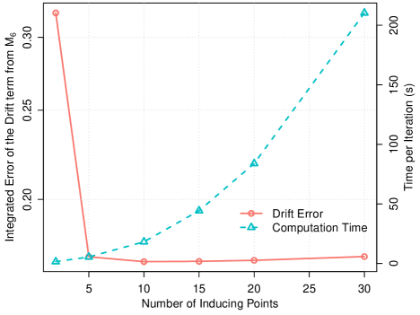
Figure 1: Drift’s integrated error and computational time per iteration depending on $m$ for a small subset of $M_{6}$ simulations.

Based on these results, we run our SGP method using $m=2,5,10$ and $15$. It should be noted that $m<<N$ and hence, we could have used larger $m$ without compromising the computational tractability of the problem. Also note that although Fig. 1 suggests that we could stop searching at $m=10$, we have also included $m=15$. This was done to compare both estimates and further investigate the impact of $m$ in the lower bound. Furthermore, Fig. 1 was obtained using a small subset of the data from a single model and, therefore, there may be simulations for which the use of $m=15$ may yield better estimates.

For each value of $m$, several trials with randomly selected initial values of the hyperparameters were run. The length-scales of both drift and diffusion kernels were restricted to the interval $l\in[0.25,2]$, based again on the fact that all the time series have a range of the order of 1. The value $A_{f}$ was set to 25 (equivalent to a standard deviation of 5) and the initial value of $\theta_{f,0}$ was randomly initialized into the interval $[0,A_{f}]$. The selection of $v$ and the amplitude hyperparameter for the diffusion process was made using Eq. (24) and $A_{g}=25$ for all the models present in the simulated set. The starting values for the pseudo-inputs were selected using the percentile initialization. The final model for each of the time series was selected by using the modified lower bound (Eq. (22)).

Table 2 summarises the mean values of the integrated errors for all the models from Table 1. The best result for each model is marked in bold (smaller is better) . Additionally, a star (*) points those best-results with statistically significant differences with respect to the other two methods. The differences between methods were tested using the Nemenyi post-hoc test Nemenyi (1962). The results in Table 2 show that our proposal has a good performance, specially in the drift estimates, where it performs better than KBR and POLY in the majority of the models. The results for the diffusion are also good, but the SGP method has the largest mean error for the $M_{5}$ model. The reason for this is discussed below.

Table 1: Models used for the validation with synthetic data.

Model	$f(x)$	$\sqrt{g(x)}$
$M_{1}$	$-(x-3)$	$\sqrt{2}$
$M_{2}$	$-(x^{3}-x)$	$1$
$M_{3}$	$-x^{3}$	$0.2+x^{2}$
$M_{4}$	$-0.7(x-0.5)$	$\sqrt{0.7x(1-x)}$
$M_{5}$	$-(x-0.225)$	$0.5\sqrt{x}$
$M_{6}$	$-x+\sin(3.5*x)\exp(-x^{2})$	$0.431$

Table 2: Integrated absolute errors of the methods KBR and POLY and our proposal (denoted as SGP), using different test models with length $N=10^{4}$.

	Drift estimates			Diffusion Estimates
Model	YYYKBR	YYYPOLY	YYYSGP	YYYKBR	YYYPOLY	YYYSGP
$M_{1}$	$0.6863$	$0.7896$	$0.4992*$	$0.03963$	$0.03426$	$0.02684*$
$M_{2}$	$0.5073*$	$0.6267$	$0.5760$	$0.01915$	$0.01878$	$0.01511*$
$M_{3}$	$0.1501$	$0.2731$	$0.1232*$	$0.05293$	$0.02711$	$0.007465*$
$M_{4}$	$0.1244$	$0.1519$	$0.1128*$	$0.02585$	$0.002054*$	$0.0045$
$M_{5}$	$0.09035$	$0.1613$	$0.08256*$	$0.001338*$	$0.001771$	$0.002667$
$M_{6}$	$0.2289$	$0.2618$	$0.2256$	$0.002751$	$0.002972$	$0.002323*$

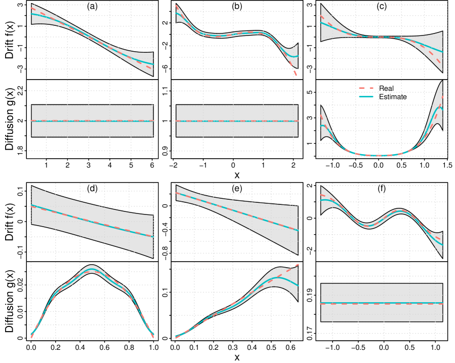
Figure 2: Drift and diffusion estimates obtained from a single trajectory of the simulated models: (a) $M_{1}$, (b) $M_{2}$, (c) $M_{3}$, (d) $M_{4}$, (e) $M_{5}$ and (f) $M_{6}$. The shaded area represents the 95% confidence region.

Fig. 2 illustrates the kind of estimates that the SGP method yields for the drift and diffusion terms from a single realization of the simulated models. Note that the confidence intervals (grey regions) usually increase when $x$ takes extreme values. This is due to the fact that the regions where $x$ takes extreme values are only visited a few times during any simulated trajectory and hence only a few points are available for the estimation. Since there is little data at these regions, the priors have strong influence and the estimates tend to curve towards the prior means. This effect is particularly remarkable for the drift estimates, which curve towards zero, and the diffusion for $M_{5}$. This is probably the reason why the SGP method does not perform as well as expected for the diffusion for $M_{5}$ and the drift for $M_{2}$.

Concerning the selected number of pseudo-inputs $m$, the general trend is that $\mathcal{L^{\prime}}$ (see Eq. (22)) increases with $m$, as we might have expected (see Section V.1). Hence, all the selected models use $m=15$ inducing points. However, it is not always worth to increase $m$ in terms of the integrated error versus the running time, which scales as $\mathcal{O}(2^{m})$ due to the use of the L-BFGS-B algorithm (see Fig. 1). This can be understood by looking at Fig. 3. The figure shows two estimates of the $M_{5}$’s diffusion term obtained using a different number of inducing-points, which are also represented in the plot. As noted with Fig. 2, the width of the confidence intervals (grey regions), depends on the number of points available for the estimation, illustrated with the point cloud. The similarity between both estimates over the high-density region results in an almost identical weighted integrated error. However, the $\mathcal{L^{\prime}}$ is larger for $m=15$ than for $m=10$, mostly because the confidence interval significantly increases in the low-density region for $m=10$. The use of additional inducing-points in the case $m=15$ permits a better control of the estimates and the confidence interval, which results in a larger $\mathcal{L^{\prime}}$ although the weighted integrated error is very similar. Hence, the $\mathcal{L^{\prime}}$ based selection criteria is not optimal for the purpose of minimizing the weighted integrated error without wasting computational resources. From these experimental results about the impact of $m$ in $\mathcal{L^{\prime}}$ we conclude the selection of $m$ should not be based solely on the lower bound, since it monotically increases with $m$ at a cost of greater computation times. Therefore, we suggest adopting Rasmussen’s heuristic (Section V.1) in combination with $\mathcal{L^{\prime}}$, using Eq. (25) as an initial guess for the value of $m$.

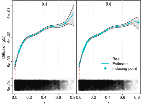
Figure 3: Diffusion estimates obtained using (a) $m=10$ and (b) $m=15$ inducing points. The density of the point cloud at the bottom of the figure represents the number of points available for the estimation at each $x$.

VII Application to real data

VII.1 Financial data

In this Section, we apply our method to a real time series from econophysics with the aim of illustrating the applicability of SDEs to non-stationary problems and the role that non-constant diffusions play in complex dynamics. We study the daily fluctuations in the oil price in the period 1982/01/02-2017/05/30, which results in a time series $\bm{p}$ of length $N\approx 10^{4}$ U.S. Energy Information Administration (2017). Following Ghasemi et al. (2007), we constructed the daily logarithmic increments of the oil price $x_{n}=\log p_{n+1}/p_{n}$ to obtain a stationary time series. The SGP method was then applied using $m=10$ inducing points (randomly started using the percentile initialization) and two squared exponential kernels. The numerical stability of the kernels was improved using Eq. (28). The amplitudes of the kernels were selected to match a standard deviation of 5 for both the drift and diffusion functions. The algorithm was run several times with random initial values for the length-scales. The final estimates selected using the lower bound are shown in Fig. 4. These estimates are in good agreement with those reported in Ghasemi et al. (2007) (although this work focused in a smaller period). Similar estimates are also obtained using the KBR and POLY methods.

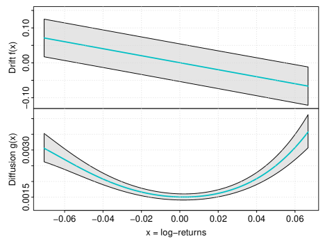
Figure 4: Drift and diffusion estimates obtained with the SGP method on the oil price log-returns.

The drift and diffusion functions shown in Fig. 4 can be approximated by $\hat{f}(x)\approx-x$ and $\hat{g}(x)\approx D+\gamma x^{2}$, which yields the SDE of a quadratic-noise Ornstein-Uhlenbeck process (Gillespie, 1991, Chapter 3). This process is an illustrative example of the effects that multiplicative noise may have in the dynamics of a system. The stationary distribution of a quadratic-noise Ornstein-Uhlenbeck process is a non-standardized Student’s distribution, which is a heavy-tailed distribution that permits the occurrence of large values in the log-returns series. Furthermore, this stationary distribution is more closely confined to the origin in comparison with the standard Ornstein-Uhlenbeck noise, which implies that the stable state is narrower in the quadratic case. This is an example of noise-enhanced stability (Gillespie, 1991, Chapter 3) and illustrates the importance that the non-parametric estimation of the diffusion may have in the study of complex dynamics.

VII.2 Paleoclimatology data

In this Section, we apply our estimation algorithm to a real data problem related to paleoclimatology. Climate records from the Greenland ice cores have played a central role in the study of the Earth’s past climate in the Northern hemisphere. Among other interesting phenomena, these records show abrupt rapid climate fluctuations that occurred during the last glacial period, which ranges from approximately 110 Ky (1 Ky = 1000 years) to 12 Ky before present. These abrupt climate changes are usually referred to as Dansgaard-Oeschger (DO) events. Although there seems to be a general agreement that DO events are transitions between two quasi-stationary states (the glacial or stadial and the interstadial states), it is still actively debated the nature of the phenomena triggering the transitions. It has been argued that the DO events occur quasi-periodically with a recurrence time of approximately 1.47 Ky Schulz (2002). However, recent studies support that the DO events are probably noise induced Ditlevsen et al. (2007); Ditlevsen and Ditlevsen (2009); Krumscheid et al. (2015).

We apply our method to the $\delta^{18}\text{O}$ record during the last glacial period obtained from the North Greenland Ice Core Project (NGRIP) Andersen et al. (2004). The $\delta^{18}\text{O}$ is a measure of the ratio of the stable isotopes oxygen-18 and oxygen-16 which is commonly used to estimate the temperature at the time that each small section of the ice core was formed. It is measured in “permil” (‰, parts per thousand) and its formula is:

$$\delta^{18}\text{O}=\Bigg{(}\frac{\left[\frac{{}^{18}\text{O}}{{}^{16}\text{O}}\right]_{\text{sample}}}{\left[\frac{{}^{18}\text{O}}{{}^{16}\text{O}}\right]_{\text{reference}}}-1\Bigg{)}\cdot 1000\text{ \permil},$$

where reference defines a well-known isotopic composition.

Fig. 5 shows the oxygen isotopic composition from the NGRIP ice core. We consider the period ranging from 70 Ky to 20 Ky before present as in Krumscheid et al. (2015), since it is dominated by the DO events, as can be clearly observed.

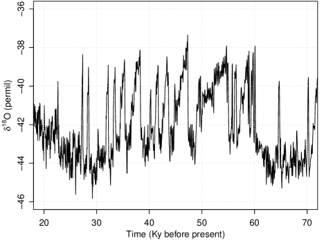
Figure 5: DO transitions during the last glacial period.

We applied our method using different kernels to illustrate that different covariance functions can be used and combined to create different models, and that Eq. (22) can be used to select the best among them. Within our method, testing different kernels is important because we usually do not have enough information about the drift and diffusion terms to decide among them. Furthermore, the performance of GPs depends almost exclusively on the suitability of the chosen kernel to capture the features of the modelled function. Consider the following illustrative example: a function with fast quasi-periodic oscillations superimposed on a linear trend. A squared exponential kernel with a large length-scale can capture the behaviour of the linear slope and make reasonable predictions of the trend for unobserved values, but it won’t be able to model the quick wiggles. On the other hand, a squared exponential kernel with a small length-scale will be able to accurately fit all the data but, since the distance from the training points rapidly increases, it won’t be able to make good predictions for unobserved values, not even for the trend. Furthermore, the uncertainty of the unobserved values will also scale fast. A better covariance choice could make use of a sum of exponential kernels with different length-scales, which would permit to accurately fit the data and make good predictions for the trend. More complex kernel choices are also possible. For a complete example on the impact of the kernel in the modelling capabilities of a GP, see (Rasmussen and Williams, 2006, Chapter 5). For our illustrative example on the paleoclimate data, we used the kernel specified in Eq. (27), a sum of two exponential kernels with different length-scales and a rational quadratic kernel. All these kernels were modified adding a small value to their main diagonals as in Eq. (28).

For each possible kernel, the method was started with random values for the hyperparameters. The number of the pseudo-inputs was set to $m=15$, based on the good results that it achieved at Section VI. The amplitudes of the kernels were selected so that they were compatible with a standard deviation of 30 for both the drift and diffusion functions. The estimates selected based on the value of the modified lower bound (Eq. (22)) are illustrated in Fig. 6. The drift term was obtained using a rational squared kernel whereas the diffusion term was estimated using the kernel from Eq. (27). Note that, as expected, the drift function presents two stable points: one corresponding to the stadial state and the other corresponding to the interstadial state. Integrating the drift function yields the potential function, which indicates that the stadial state corresponds to a stable state of the system since it has the lowest energy. On the other hand, the interstadial state corresponds to a metastable state.

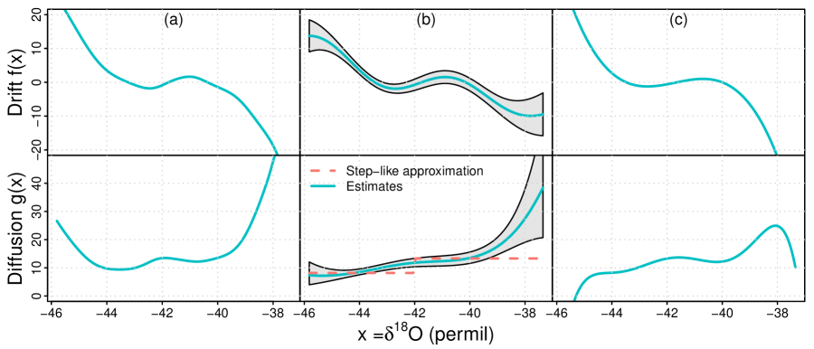
Figure 6: Best drift and diffusion estimates using the (a) KBR, (b) SGP and (c) POLY methods with the paleoclimate data.

The SGP estimate supports the use of a state-dependent diffusion rather than the widely-used constant term. The use of a state-dependent diffusion for the DO events was first proposed in Krumscheid et al. (2015), which suggested:

$$f(x,\bm{\theta})=\sum_{i=0}^{3}\theta_{j}x^{j};\qquad g(x,\bm{\theta})=\begin{cases}\theta_{4}\text{ if }x<\theta_{6}\\ \theta_{5}\text{ if }x\geq\theta_{6}\end{cases}.$$ (29)

Krumscheid et al. suggested the model from Eq. (29) while testing their framework for parametric inference and model selection for SDEs Krumscheid et al. (2015). The authors discussed the model from Eq. (29) since it is able to accurately predict the histogram of the DO events, although the final parametrization that results from their model selection criteria proposes a constant diffusion term. However, our non-parametric methodology suggests that the state dependent diffusion is indeed preferable. Despite it is possible to approximate the SGP diffusion’s estimate using a step function (as can be appreciated in Fig. 6), there exists a linear increasing region for $x>-40$ that does not match Krumscheid’s model. To compare the diffusion model in Ref. Krumscheid et al. (2015) with the SGP’s diffusion model, a Lasso estimate De Gregorio and Iacus (2012) was applied to the diffusion term while keeping the drift term fixed. Lasso penalties are very useful in regression analysis since they are able to set coefficients to zero, eliminating unnecessary variables. Hence, by using the diffusion term:

$$g(x,\bm{\theta})=\begin{cases}\theta_{1}\text{ if }x<-42\\ \theta_{2}\text{ if }-42\leq x<-40\\ \theta_{2}+\theta_{3}(x+40)\text{ if }x\geq-40\end{cases},$$ (30)

we can compare the model proposed in Krumscheid et al. (2015) (which corresponds with setting $\theta_{3}=0$) and our estimate. The Lasso estimate provides evidence in favour of the model obtained through our method, since the $\theta_{3}$ is not eliminated. Note, however, that this evidence it is not conclusive since the time series used for the estimates is quite short ($N\approx 10^{3}$) and there is a lack of points for $x>-39$.

We have also used the SGP estimates to compute the distribution of the time between DO events. 1000 new time series were generated using the Euler-Maruyama scheme. The initial points were sampled with replacement from the real paleoclimate series. To robustly identify the DO states, we fitted a Hidden Markov Model (HMM) with three states and Gaussian response to the real data. The aim of the three states is to clearly identify the stadial state, the interstadial state and a “transition state”. We identified the states of each of the simulated time series using this HMM by means of the Viterbi algorithm Viterbi (1967). The resulting mean time between DO events was 1.50 Ky, in good agreement with the generally accepted value of 1.47 Ky Schulz (2002). However, it must be noted that this value was obtained on basis of a quasi-periodical model, whereas our value is based on a stochastic model.

Using the KBR (Fig. 6) and POLY (Fig. 6) methods result in similar drift estimates, compared with the SGP one. Furthermore, both diffusion estimates also support the use of a the state-dependent model. However, the SGP estimate provides confidence intervals based on a Bayesian setting while the others methods do not. Also, the KBR method presents an unlikely increment in the diffusion for $x<-44$. The POLY method approximates the shape of the state-dependent diffusion using a high order polynomial, which cannot properly capture the plateau for $x<-44$. Additionally, the polynomial fit results in negative values for $x<-45$ which have no sense for a diffusion term.

VIII Discussion and conclusions

In this paper, we have presented a non-parametric estimation method for SDEs from densely-observed time series based on GPs. The only assumptions made on the data are that they fulfil the Markovian condition and that the sampling period is small enough so that the Euler-Maruyama discretization holds. From the point of view of the adoption of GPs to the estimation of SDEs, the main contributions of this paper are: (1) providing estimates for any type of diffusion function and (2) proposing a sparse approximation to the true GP posterior that permits to efficiently handle the typical experimental time series size of $N\approx 10^{3}-10^{5}$. To cope with the computational complexity of calculating the posterior distribution of the GPs (which scales as $\mathcal{O}(N^{3})$), we approximate the GPs using the evidence provided by the data in only a small set of function points, the inducing variables. The inducing variables are learnt by minimizing the Kullback-Leibler divergence between the true posterior GP distribution and the approximated one. The minimization problem is approached using the standard techniques from the variational inference framework, which usually yields a coordinate-ascent optimization to approximate the posterior. However, our approach makes use of a non conjugate model due to the inclusion of the diffusion function, which prevents the direct use of variational inference methods. To tackle the problem, a Laplace approximation was used to compute the distribution modelling the diffusion. It must be noted that, although we have developed our estimation approach bearing in mind the computational challenges that a large $N$ imposes, our proposal can also handle small time series without any further adjustment. Also, although the SGP approximation permits handling large experimental time series, $N$ cannot increase without limit. Variational inference algorithms require a full pass through the whole dataset at each iteration and hence, they become inefficient for massive datasets, even when using sparse techniques like the proposed one. For example, in a computer with an Intel Xeon E5-2650L at 2.05 GHz and using $m=10$, the computation time increases from 8 minutes per iteration with $N=10^{5}$ to 1.4 hours per iteration with $N=10^{6}$. Scaling up variational inference can be done using stochastic gradient optimization, which yields stochastic variational inference Hoffman et al. (2013). Since large datasets are increasingly common, the use of this kind of techniques should be considered in future work.

The performance of the SGP estimates was evaluated using simulated data from different SDE models and compared with the kernel based method Lamouroux and Lehnertz (2009) and the polynomial based method Rajabzadeh et al. (2016). The results show that the SGP approach is able to provide very accurate estimates, specially for the drift term. The main advantage of the SGP method with respect to Lamouroux and Lehnertz (2009) and Rajabzadeh et al. (2016) is that it permits a Bayesian treatment of the estimation problem; this enables obtaining probabilistic predictions and computing robust confidence intervals. Furthermore, the prior information about the drift/diffusion is expressed in a function-space view, i.e., the SGP method permits specifying the prior directly over functions instead of working with weights of some basis expansion. In our view, this is a more natural way of working with functions. Another major advantage of the proposed method is its versatility. Although we have focused on very flexible kernels, any type of kernel (or even combinations of them) can be used, which may completely change the properties of the posterior estimates. For example, using polynomial kernels would yield similar estimates to those of Rajabzadeh et al. (2016), but with the aforementioned advantages of the Bayesian framework and without the possibility of obtaining negative values for the diffusion (see Section VII).

We applied the SGP method to a real problem in econophysics with the aim of illustrating the importance of non-constant diffusions in the behaviour of a system and, hence, the importance of its non-parametric estimation. This example also emphasizes the applicability of the SDE framework to non-stationary time series.

The proposed method was also applied to a real paleoclimate time series: the NGRIP core data showing the DO events occurring during the last glacial period. The SGP method accurately captures the relevant physical states of the time series (the stadial and interstadial states) and yields a mean transition time between DO events that it is close to the accepted value in the literature under the assumption of a deterministic periodic model. This demonstrates its ability to capture the behaviour of real data with complex dynamics. Furthermore, the SGP estimates provide evidence supporting a novel state dependent diffusion model for the DO events. This diffusion model is similar to the step-like function proposed in Krumscheid et al. (2015) for a wide range of the diffusion’s support, but it also adds a linear term for the region corresponding to the most extreme values of the DO events. These results should be viewed with caution, since the estimates were made using small amounts of data. Further research to assess the physical meaning of the model should be made.

In future work we would like to design some criteria to automatically estimate an appropriate number of pseudo-inputs $m$ taking into account both the modified lower bound (Eq. (22)) and the additional computational time required when $m$ increases. The substitution of the exponential transformation used to ensure the positiveness of $g$ in favour of another less-explosive transformation should also be considered in future improvements. The numerical stability of the method would certainly improve with the use of smoother transformations, but the formal expressions required for the variational inference problem would be more complicated. An alternative to avoid the complicated mathematical expressions would be to use black-box variational inference frameworks Titsias RC AUEB and Lázaro-Gredilla (2015). Since black-box methods are based in stochastic variational inference, its application would also permit to scale the exposed methodology to datasets much bigger that those studied in this article. Hence, The application of black-box methods to the reconstruction of SDEs looks promising and should be explored in future work.

We believe that the presented method could help to further comprehend the dynamics underlying a wide variety of complex systems. To that end, we provide an open-source implementation of our method which is freely available at github (https://github.com/citiususc/voila).

Appendix A Variational distribution for the drift

We start expanding the expression inside the expectation operator from Equation (12a):

$$\begin{split}\log\phi_{f_{m}}(\bm{f}_{m})=&\mathbb{E}_{\phi_{\text{-}f_{m}}}\left[\log\left(p(\bm{x}|\bm{f},\bm{s})p(\bm{s}_{m})p(\bm{f}_{m})\right)\right]\\ =&\mathbb{E}_{\phi_{\text{-}f_{m}}}\left[\log p(\bm{x}|\bm{f},\bm{s})\right]+\mathbb{E}_{\phi_{\text{-}f_{m}}}\left[\log p(\bm{s}_{m})\right]\\ &+\mathbb{E}_{\phi_{\text{-}f_{m}}}\left[\log p(\bm{f}_{m})\right].\end{split}$$

Given that the expectation operator does not affect $\log p(\bm{f}_{m})$ and that when applied to $\log p(\bm{s}_{m})$ results in an expression that does not depend on $\bm{f}_{m}$, we may write:

$$\begin{split}\log\phi_{f_{m}}(\bm{f}_{m})=&\mathbb{E}_{\phi_{\text{-}f_{m}}}\left[\log p(\bm{x}|\bm{f},\bm{s})\right]\\ &-\frac{1}{2}\bm{f}_{m}^{T}\bm{K}_{mm}^{-1}\bm{f}_{m}+\text{constant},\end{split}$$ (31)

where we have denoted all terms that do not depend on $\bm{s}_{m}$ as constant. It is convenient to work with the term constant, given that we can infer its value after identifying the distribution of $\phi_{f_{m}}$. In that case, constant corresponds to the normalizing constant required by the distribution $\phi_{f_{m}}$.

Expanding the expression inside the expectation operator from Eq. (31) and joining new constants yields:

$$\log\phi_{f_{m}}(\bm{f}_{m})= -\frac{1}{2\Delta t}\sum_{i=1}^{N} \mathbb{E}_{\phi_{s_{m}}(\bm{s}_{m})p(\bm{s}\mid\bm{s}_{m})}\left[\exp(-s_{i})\right]$$ (32)

$$\times\mathbb{E}_{p(\bm{f}\mid\bm{f}_{m})}\left[(\Delta x_{i}-\Delta tf_{i})^{2}\right]$$

$$-\frac{1}{2}\bm{f}_{m}^{T}\bm{K}_{mm}^{-1} \bm{f}_{m}+\text{constant}.$$

Using Fubini’s rule of integration we may write the first expectation from Eq. 32 as:

$$\mathbb{E}_{\phi_{s_{m}}(\bm{s}_{m})p(\bm{s}\mid\bm{s}_{m})}\left[\exp(-s_{i})\right]=\mathbb{E}_{\phi_{s_{m}}}\big{[}\mathbb{E}_{p(\bm{s}\mid\bm{s}_{m})}\left[\exp(-s_{i})\right]\big{]}.$$ (33)

It is possible to demonstrate that if $X\sim\mathcal{N}(\mu,\sigma^{2})$, $\mathbb{E}\left[\exp(-X)\right]=\exp(-\mu+\sigma^{2}/2)$. Hence, Eq. (33) becomes:

$$\begin{split}\mathbb{E}_{\phi_{s_{m}}}&\big{[}\mathbb{E}_{p(\bm{s}\mid\bm{s}_{m})}\left[\exp(-s_{i})\right]\big{]}=\\ &\mathbb{E}_{\phi_{s_{m}}}\left[-[\bm{v}^{N}+\bm{B}(\bm{s}_{m}-\bm{v}^{m})]_{i}\right]+\frac{Q_{ii}}{2}=\zeta_{i},\end{split}$$ (34)

where we have used the definition of $\zeta_{i}$ from Eq. (14) and the definitions of B and Q from Eq. (8). Introducing back Eqs. (33) and (34) into Eq. (32) we finally arrive to:

$$\log\phi_{f_{m}}(\bm{f}_{m}) =-\frac{1}{2\Delta t}\sum_{i=1}^{N}\zeta_{i}\cdot\mathbb{E}_{p(\bm{f}\mid\bm{f}_{m})}\left[(\Delta x_{i})^{2}-2\Delta t\Delta x_{i}f_{i}-(\Delta t)^{2}f_{i}^{2}\right]-\frac{1}{2}\bm{f}_{m}^{T}\bm{K}_{mm}^{-1}\bm{f}_{m}+\text{constant}$$

$$=-\frac{1}{2\Delta t}\sum_{i=1}^{N}\zeta_{i}\cdot\left[(\Delta x_{i})^{2}-2\Delta t\Delta x_{i}[\bm{A}\bm{f}_{m}]_{i}-(\Delta t)^{2}([\bm{A}\bm{f}_{m}]_{i}^{2}+P_{ii})\right]-\frac{1}{2}\bm{f}_{m}^{T}\bm{K}_{mm}^{-1}\bm{f}_{m}+\text{constant}$$ (35)

Reordering Eq. (35) an expressing it in vectorial form, we recover Eq. (13).

Appendix B Variational distribution for the diffusion

Starting from Eq. (12b) and proceeding similarly to Appendix A it is possible to arrive to:

$$\log \phi_{s_{m}}(\bm{s}_{m})=$$ (36)

$$-\frac{1}{2}(\bm{s}_{m}- \bm{v}^{m})^{T}\bm{J}_{mm}^{-1}(\bm{s}_{m}-\bm{v}^{m})$$

$$-\frac{1}{2\Delta t}\sum_{i=1}^{N} \mathbb{E}_{p(\bm{s}\mid\bm{s}_{m})}\left[\exp(-s_{i})\right]$$

$$\times\mathbb{E}_{\phi_{f_{m}}(\bm{f}_{m})p(\bm{f}\mid\bm{f}_{m})}\left[(\Delta x_{i}-\Delta tf_{i})^{2}\right]$$

$$-\frac{1}{2}\sum_{i=1}^{N} \mathbb{E}_{p(\bm{s}\mid\bm{s}_{m})}\left[s_{i}\right]+\text{constant}.$$

The expectation of $\exp(-s_{i})$ can be computed as in Appendix A (see Eq. (33)), which results in

$$\log \phi_{s_{m}}(\bm{s}_{m})=$$ (37)

$$-\frac{1}{2}(\bm{s}_{m}- \bm{v}^{m})^{T}\bm{J}_{mm}^{-1}(\bm{s}_{m}-\bm{v}^{m})$$

$$-\frac{1}{2\Delta t}\sum_{i=1}^{N} \exp\bigg{(}-[\bm{v}^{N}+\bm{B}(\bm{s}_{m}-\bm{v}^{m})]_{i}+\frac{Q_{ii}}{2}\bigg{)}$$

$$\times\mathbb{E}_{\phi_{f_{m}}(\bm{f}_{m})p(\bm{f}\mid\bm{f}_{m})}\left[(\Delta x_{i}-\Delta tf_{i})^{2}\right]$$

$$-\frac{1}{2}\sum_{i=1}^{N} [\bm{B}(\bm{s}_{m}-\bm{v}^{m})]_{i}+\text{constant}.$$

Using again Fubini’s law, we may write:

$$\mathbb{E}_{\phi_{f_{m}}(\bm{f}_{m})p(\bm{f}\mid\bm{f}_{m})} \left[(\Delta x_{i}-\Delta tf_{i})^{2}\right]$$

$$=\mathbb{E}_{\phi_{f_{m}}} \left[\mathbb{E}_{p(\bm{f}\mid\bm{f}_{m})}\left[(\Delta x_{i}-\Delta tf_{i})^{2}\right]\right]$$

$$=\mathbb{E}_{\phi_{f_{m}}} \left[\Delta x_{i}^{2}\right.-2\Delta t\Delta x_{i}[\bm{A}\bm{f}_{m}]_{i}$$

$$\left.+(\Delta t)^{2}\left([\bm{A}\bm{f}_{m}]_{i}^{2}+P_{ii}\right)\right]=\psi_{i},$$

where we have used the definition of $\psi_{i}$ from Eq. (17). Introducing $\psi_{i}$ into Eq. (37), we finally arrive to Eq. (16).

References

- Langevin (1908) P. Langevin, CR Acad. Sci. Paris 146, 530 (1908).
- Lançon et al. (2001) P. Lançon, G. Batrouni, L. Lobry, and N. Ostrowsky, EPL (Europhysics Letters) 54, 28 (2001).
- Friedrich and Peinke (1997a) R. Friedrich and J. Peinke, Physica D: Nonlinear Phenomena 102, 147 (1997a).
- Friedrich and Peinke (1997b) R. Friedrich and J. Peinke, Physical Review Letters 78, 863 (1997b).
- Mekkaoui (2013) A. Mekkaoui, Physics of plasmas 20, 010701 (2013).
- Kelly et al. (2009) B. C. Kelly, J. Bechtold, and A. Siemiginowska, The Astrophysical Journal 698, 895 (2009).
- Gillespie (2007) D. T. Gillespie, Annu. Rev. Phys. Chem. 58, 35 (2007).
- Mahnke et al. (2005) R. Mahnke, J. Kaupužs, and I. Lubashevsky, Physics Reports 408, 1 (2005).
- Ghasemi et al. (2007) F. Ghasemi, M. Sahimi, J. Peinke, R. Friedrich, G. R. Jafari, and M. R. R. Tabar, Physical Review E 75, 060102 (2007).
- Ozbudak et al. (2002) E. M. Ozbudak, M. Thattai, I. Kurtser, A. D. Grossman, and A. Van Oudenaarden, Nature genetics 31, 69 (2002).
- Bahraminasab et al. (2009) A. Bahraminasab, F. Ghasemi, A. Stefanovska, P. McClintock, and R. Friedrich, New journal of physics 11, 103051 (2009).
- Friedrich et al. (2011) R. Friedrich, J. Peinke, M. Sahimi, and M. R. R. Tabar, Physics Reports 506, 87 (2011).
- Hegger and Stock (2009) R. Hegger and G. Stock, The Journal of chemical physics 130, 034106 (2009).
- Lamouroux and Lehnertz (2009) D. Lamouroux and K. Lehnertz, Physics Letters A 373, 3507 (2009).
- Rajabzadeh et al. (2016) Y. Rajabzadeh, A. H. Rezaie, and H. Amindavar, Physica A: Statistical Mechanics and its Applications 450, 294 (2016).
- Rasmussen and Williams (2006) C. Rasmussen and C. Williams, Gaussian Processes for Machine Learning, Adaptive Computation and Machine Learning (MIT Press, Cambridge, MA, USA, 2006) p. 248.
- Ruttor et al. (2013) A. Ruttor, P. Batz, and M. Opper, in Advances in Neural Information Processing Systems (2013) pp. 2040–2048.
- Quiñonero-Candela and Rasmussen (2005) J. Quiñonero-Candela and C. E. Rasmussen, Journal of Machine Learning Research 6, 1939 (2005).
- Gammaitoni et al. (1998) L. Gammaitoni, P. Hänggi, P. Jung, and F. Marchesoni, Reviews of modern physics 70, 223 (1998).
- Pikovsky and Kurths (1997) A. S. Pikovsky and J. Kurths, Physical Review Letters 78, 775 (1997).
- Horsthemke (1984) W. Horsthemke, in Non-Equilibrium Dynamics in Chemical Systems (Springer, 1984) pp. 150–160.
- Iacus (2009) S. M. Iacus, Simulation and inference for stochastic differential equations: with R examples (Springer Science & Business Media, 2009).
- Kloeden and Platen (1999) P. E. Kloeden and E. Platen, Numerical solution of stochastic differential equations, Applications of mathematics (Springer, Berlin, New York, 1999).
- Lind et al. (2005) P. G. Lind, A. Mora, J. A. Gallas, and M. Haase, Physical Review E 72, 056706 (2005).
- Kuusela (2004) T. Kuusela, Physical Review E 69, 031916 (2004).
- Prusseit and Lehnertz (2008) J. Prusseit and K. Lehnertz, Physical Review E 77, 041914 (2008).
- Murphy (2012) K. P. Murphy, Machine learning: a probabilistic perspective (MIT press, 2012).
- Titsias (2009) M. K. Titsias, in AISTATS, Vol. 12 (2009) pp. 567–574.
- Bishop (2006) C. M. Bishop, Pattern Recognition and Machine Learning (Information Science and Statistics) (Springer-Verlag New York, Inc., 2006).
- Wang and Blei (2013) C. Wang and D. M. Blei, Journal of Machine Learning Research 14, 1005 (2013).
- Byrd et al. (1995) R. H. Byrd, P. Lu, J. Nocedal, and C. Zhu, SIAM Journal on Scientific Computing 16, 1190 (1995).
- McLachlan and Krishnan (2007) G. McLachlan and T. Krishnan, The EM algorithm and extensions, Vol. 382 (John Wiley & Sons, 2007).
- Blei et al. (2017) D. M. Blei, A. Kucukelbir, and J. D. McAuliffe, Journal of the American Statistical Association (2017).
- Duvenaud (2014) D. Duvenaud, Automatic model construction with Gaussian processes, Ph.D. thesis, University of Cambridge (2014).
- Larsen and Sørensen (2007) K. S. Larsen and M. Sørensen, Mathematical Finance 17, 285 (2007).
- Cox et al. (1985) J. C. Cox, J. E. Ingersoll Jr, and S. A. Ross, Econometrica: Journal of the Econometric Society , 385 (1985).
- Silverman (1986) B. W. Silverman, Density estimation for statistics and data analysis, Vol. 26 (CRC press, 1986).
- Kennedy and Gentle (1980) J. Kennedy, William J. and J. E. Gentle, Statistical computing (Marcel Dekker Inc, New York, 1980).
- Note (1) For further reproducibility, the parameters inferred in the algorithm can be found at https://github.com/citiususc/voila/blob/master/additional_material/synthetic_data_parameters.txt.
- Nemenyi (1962) P. Nemenyi, in Biometrics, Vol. 18 (International Biometric Society, 1962) p. 263.
- U.S. Energy Information Administration (2017) U.S. Energy Information Administration, “Crude oil prices from https://www.eia.gov/dnav/pet/pet_pri_spt_s1_d.htm,” (2017).
- Gillespie (1991) D. T. Gillespie, Markov processes: an introduction for physical scientists (Elsevier, 1991).
- Schulz (2002) M. Schulz, Paleoceanography 17 (2002).
- Ditlevsen et al. (2007) P. D. Ditlevsen, K. K. Andersen, and A. Svensson, Climate of the Past 3, 129 (2007).
- Ditlevsen and Ditlevsen (2009) P. D. Ditlevsen and O. D. Ditlevsen, Journal of Climate 22, 446 (2009).
- Krumscheid et al. (2015) S. Krumscheid, M. Pradas, G. Pavliotis, and S. Kalliadasis, Physical Review E 92, 042139 (2015).
- Andersen et al. (2004) K. K. Andersen, N. Azuma, J.-M. Barnola, M. Bigler, P. Biscaye, N. Caillon, J. Chappellaz, H. B. Clausen, D. Dahl-Jensen, H. Fischer, et al., Nature 431, 147 (2004).
- De Gregorio and Iacus (2012) A. De Gregorio and S. M. Iacus, Econometric Theory 28, 838 (2012).
- Viterbi (1967) A. Viterbi, IEEE transactions on Information Theory 13, 260 (1967).
- Hoffman et al. (2013) M. D. Hoffman, D. M. Blei, C. Wang, and J. Paisley, The Journal of Machine Learning Research 14, 1303 (2013).
- Titsias RC AUEB and Lázaro-Gredilla (2015) M. Titsias RC AUEB and M. Lázaro-Gredilla, in Advances in Neural Information Processing Systems 28, edited by C. Cortes, N. D. Lawrence, D. D. Lee, M. Sugiyama, and R. Garnett (Curran Associates, Inc., 2015) pp. 2638–2646.