Point Sweep Coverage on Path

Abstract

An important application of wireless sensor networks is the deployment of mobile sensors to periodically monitor (cover) a set of points of interest (PoIs). The problem of Point Sweep Coverage is to deploy fewest sensors to periodically cover the set of PoIs. For PoIs in a Eulerian graph, this problem is known NP-Hard even if all sensors are with uniform velocity. In this paper, we study the problem when PoIs are on a line and prove that the decision version of the problem is NP-Complete if the sensors are with different velocities. We first formulate the problem of Max-PoI sweep coverage on path (MPSCP) to find the maximum number of PoIs covered by a given set of sensors, and then show it is NP-Hard. We also extend it to the weighted case, Max-Weight sweep coverage on path (MWSCP) problem to maximum the sum of the weight of PoIs covered. For sensors with uniform velocity, we give a polynomial-time optimal solution to MWSCP. For sensors with constant kinds of velocities, we present a $\frac{1}{2}$-approximation algorithm. For the general case of arbitrary velocities, we propose two algorithms. One is a $\frac{1}{2\alpha}$-approximation algorithm family scheme, where integer $\alpha\geq 2$ is the tradeoff factor to balance the time complexity and approximation ratio. The other is a $\frac{1}{2}(1-1/e)$-approximation algorithm by randomized analysis.

I Introduction

Coverage is one of the most important applications of wireless sensor networks (WSNs). In applications of WSN, sensors are placed in an area of interest (AoI) to monitor the environment and detect extraordinary. Coverage problem have been gotten much attention because of its importance. Many researches have been studied on this topic on various scenes, including discrete points[8], 2-dimensional surface, 3-dimensional surface[15], 3-dimensional space, fence[16] and so on. Based on sensors’ characteristic, special factors should be considered such as energy efficiency, maintaining connectivity and so on[19, 18].

However, most of the existing work mainly focus on continuous coverage, where sensors stay still after placed on the objective locations. Not until recently did sweep coverage be brought up to study the periodical coverage situation. Periodical coverage is also a typical application. For example, guards need to patrol barrier periodically where intruders need some time to cross; Information collector should collect information from the objective sensors periodically in case that their memory overflow. In those situations, the objects do not need to covered continuously. So mobile sensors can move around to cover more objects than continuous coverage to reduce monitoring cost. Therefore, sweep coverage begins to be payed attention after being brought up[2, 3, 8, 10, 17].

In this paper, we focus on the point sweep coverage problem in which a set of discrete points need to be covered by a given set of mobile sensors at least once within a given period of time. The point sweep coverage problem was first brought up in the paper[2] that showed finding minimum number of mobile sensors with a constant velocity to cover PoIs in an Eulerian graph is NP-Hard and can not be approximated within a factor of 2. Until now, there have not been papers to discuss the situation in which PoIs are sweep covered by mobile sensors with arbitrary velocities because of its hardness. Nevertheless, it is an important situation because the maximum velocities of mobile sensor would be reduced along with their energy used up. In this paper, we start to study the situation when mobile sensors have arbitrary velocities. It must be a NP-Hard problem when PoIs in graph. We want to study a simpler scene that PoIs are distributed on path. We call it point sweep coverage on path (PSCP) problem, which is to find whether or not a given set of mobile sensors cover all the PoIs on path periodically.

Point sweep coverage problem on path is a simpler scene than graph but also of good practical use. For example, as illustrated in Figure 1, numbers of static sensors are placed on key locations to collect real-time information of ocean or resources. A set of mobile sensors are given to collect the data from the static sensors periodically in case that the memory of the static sensors overflow. It is one of classic practical scene of PSCP problem. Besides, PSCP problem is of practical use in security, forest conservation, resource exploration and so on. It makes PSCP problem necessary to study.

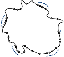
Figure 1: Mobile sensors sweep coverage around island to collect the data from the static sensors

In this paper, we prove that PSCP problem is NP-Complete and define its optimization problem, Max-Weight sweep coverage on path (MWSCP), which is NP-Hard. The MWSCP problem is to find the maximum sum of weight of PoIs covered by a given set of mobile sensors when PoIs are distributed on a path. When the weight of PoIs is one, MWSCP problem turns to be a special case, Max-PoI sweep coverage on path (MPSCP) problem, whose object is to maximum the number of PoIs sweep covered. We analyze the special cases and general case of MWSCP respectively, propose an optimal algorithm for the uniform velocity case and approximation algorithms for others.

The main contributions of this paper are summarized as follows:

• We define the point sweep coverage on path (PSCP) and its variant problems, Max-Weight sweep coverage on path (MWSCP) problem.

• We prove PSCP is NP-Complete and MWSCP is NP-Hard.

• For the special cases of MWSCP problem when sensors have uniform velocity, we present an optimal algorithm.

• For the special cases of MWSCP problem when sensors have constant number of velocities, we propose a $\frac{1}{2}$-approximation algorithm.

• For the general cases of MWSCP problem when sensors have arbitrary velocities, we propose two algorithms. One is a $\frac{1}{2\alpha}$-approximation algorithm family scheme, where integer $\alpha\geq 2$ is the tradeoff factor to balance the time complexity and approximation ratio. And the other is a $\frac{1}{2}(1-1/e)$-approximation algorithm by randomized analysis.

The rest of this paper is organized as follows: Section 2 describes some related work. In Section 3, the definition and NP-Completeness proof of the PSCP problem are given. In Section 4, we define MPSCP problem and MWSCP problem, present our optimal and approximation algorithms for different cases of MWSCP problem. Section 5 concludes the paper.

II Related work

Point sweep coverage was firstly brought up in [2].The authors presented a min-sensor point sweep coverage problem (MSPSC) to find the minimum number of sensors to sweep cover PoIs in Eulerian graph, which was proved NP-Hard by transforming TSP problem to it. The problem could not be approximated within ratio 2 and local algorithms can not work. In [5], the authors distinguished sensors’ strategies, proposed MinExpand algorithm for un-cooperated sensors and Osweep algorithm for cooperated sensors respectively. The mistake of approximation analysis of prior papers was rectified by Gorain et al.[11]. 3-approximation algorithm for MSPSC problem was proposed and it may be the best approximation algorithm for MSPSC until now. No polynomial time constant factor approximation algorithm for MSPSC was also proved. Some variants of MSPSC were also presented. When PoIs had different sweep periods, a $\mathcal{\text{O(log}\rho})$-approximation algorithm were proposed, where $\rho$ was the ratio of the maximum and minimum sweep periods among PoIs. And there were area sweep coverage problem and line sweep coverage problem proposed[9, 10], The problem of area sweep coverage are NP-Hard and a $(\sqrt{2}+\frac{2-\sqrt{2}}{mn})$-approximation algorithm for that were proposed. The line sweep coverage problem was also NP-Hard. Gorain et al. proposed a 2-approximation algorithm and proved the problem can not be approximated within 2. In [1], the effect of sensing range was considered. The authors proposed DSRS problem and proved it NP-Hard. In [12], energy consumption was taken into consideration. Two new problem were proposed. One was to minimizing energy consumption and the other was to minimizing the number of sensors when energy consumption was bounded. All the above papers only focused on the point sweep coverage problem when sensors had uniform velocity. No approximation algorithm had been brought up for sensors having different velocities yet.

Even though the point sweep coverage problem was presented firstly by [2], the concept of sweep coverage initially came from the context of robotics. The researches on robotics often focused on sweep covering continuous lines, and the problem was called boundary patrolling or fence patrolling. In these researches, the aim was to find the minimized idleness, i.e., the longest time interval during which there is at least one point on the boundary still uncovered by any mobile sensors. In [4], the authors firstly studied boundary patrolling problem and proposed two intuitional algorithms for open and close fence patrolling. The optimality of the intuitional algorithms was disproved in [6, 13, 14]. Some examples were proposed to illustrate that the idleness could be reduced to 41/42, 24/25 even 3/4 by special design, assuming the idleness of proportional solution presented in [4] is 1 . Even though the optimality of algorithms presented by Czyzowicz et al. was disproved, the optimal solution had not been brought up yet. In [17], the authors extended the scenes of the Min-idleness point sweep coverage problem to chain, tree, and cyclic roadmap. Within tolerance $\epsilon$, they could get an optimal idleness when PoIs were on chain in time complexity $O(nlog(\epsilon^{-1}))$. And a 8-approximation algorithm was proposed to find min-idleness when PoIs were on cyclic roadmap. The problem is NP-Hard. In [3], the authors described a fragmented boundaries environment and found the optimal solution for Min-idleness in that environment.

III Point sweep coverage on path

In this section, we will study PSCP problem. Firstly we present the definition of PSCP problem. Then we prove PSCP problem NP-complete.

The definition of point sweep coverage on path is given below according to the definition of point sweep coverage[2].

defn 1.

(Point Sweep Coverage on Path problem) Given a set of PoIs $P=\{p_{1},p_{2},..,p_{N}\}$ distributed on a path, each one $p_{i}$ needs to be covered every $T$ time period. If $p_{i}$ is covered within $T$ time period, then we call $p_{i}$ is $T$-sweep covered. Time period $T$ is also called sweep period. Given $M$ mobile sensors $S=\{s_{1},s_{2},..,s_{M}\}$ patrolling the $N$ PoIs, find whether the mobile sensors can sweep cover all PoIs.

Without loss of generality, when PoIs are on an open path, we can simplify that the set of PoIs are located on x-line with x-coordination $X=\{x_{1}=0,x_{2},...,x_{N}\}(x_{1}<x_{2}<...<x_{N})$. Let $V=\{v_{1},v_{2},...,v_{M}\}$ where $v_{i}$ is the velocity of sensor $s_{i}\in S$ $(1\leq i\leq M)$. PoIs have uniform sweep period $T$. Let $L$ denotes the line segment from $1^{st}$ PoI to $N^{th}$ PoI. The algorithm for open path can be easily transformed to the one for close path, so we do not belabor the algorithm for close path.

From the existing work, we know there are thousands of strategies for mobile sensors to cover PoIs and mainly be classified to 2 kinds . Between those, there is a kind of simple strategy, separated strategy, by which mobile sensors move back and forth to cover a line segment without cooperating with others and each PoI is only covered by the same mobile sensor periodically.

defn 2.

(Separated strategy)[3]. Each mobile sensor moves back and forth on the line segment, and the trajectories of different sensor do not overlap with each other.

Separated strategy is not necessarily the optimal strategy. There are complicated strategies by which some sensors cooperate with others to cover the same line segment and PoIs are sweep covered by more than one mobile sensor, which are classified as cooperated strategy. Some examples are proposed to show that separated strategy may slightly worse than some complicated strategy [6, 13] in some special cases, i.e., the covering range covered by a set of mobile sensors using separated strategy would be slightly shorter than some complicated strategy. However, until now, how to cooperate among sensors to get the optimal monitoring efficiency is still unknown.

Using separated strategy, every mobile sensor has its own covering region. The range of the region is denoted by $r_{i}$, $r_{i}\leq v_{i}T/2$ for each $s_{i}\in S$. In optimal deployment, we can just assume $r_{i}=v_{i}T/2$. Then a sensor’s trajectory can be denoted by the first PoI’s location in its covering region and its covering range. Since the covering range of a sensor has already decided by the velocity of the sensor in optimal separated strategy, we can just use the first PoI’s locations in sensors’ covering region to denote the separated deployment.

The notations will illustrated in table 1.

Table I: Notations

Symbol	Definition
$N$	the number of the PoIs
$M$	the number of the sensors
$P$	the set of PoIs $\{p_{1},p_{2},..,p_{N}\}$
$S$	the set of mobile sensors $\{s_{1},s_{2},..,s_{M}\}$
$X$	the locations of PoIs $\{x_{1},x_{2},\ldots,x_{N}\}$ $(x_{1}<x_{2}<...<x_{N})$
$T$	the uniform sweep period of PoIs
$V$	velocities of the sensors $\{v_{1},v_{2},...,v_{M}\}$
$W$	the weight of the PoIs $\{w_{1},w_{2},...,w_{N}\}$

III-A Problem Hardness

In this section, we want to prove PSCP problem NP-Complete. Before the proof, let us recall the definition of the 3-Partition problem and quote a theorem from paper[13]. Then in the proof, we will transform 3-Partition problem to PSCP problem.

defn 3.

(3-Partition)[7]

INSTANCE: Set A of 3m elements, a bound $B\in Z^{+}$, and a size $s(a)\in Z^{+}$for each $a\in A$ such that $B/4<s(a)<B/2$ and such that $\sum_{a\in A}s(a)=mB.$

QUESTION: Can A be partitioned into m disjoint sets $A_{1},A_{2},...,A_{m}$ such that, for $1\leq i\leq m$, $\sum_{a\in A_{i}}s(a)=B$ (note that each $A_{i}$ must therefore contain exactly three elements from A) ?

thm 4.

[13]For three sensors or two sensors, the separated strategy is optimal.

thm 5.

Point sweep coverage on path is NP-Complete problem.

Proof.

Given a 3-Partition instance like definition 3, we construct a PSCP instance. Given a set of $N$ PoIs, where $N=(2B+2)*m$, the positions of PoIs are $\{x_{1},x_{2},...,x_{N}\}(x_{1}<x_{2}<...<x_{N})$. $d_{i}=x_{i+1}-x_{i}(1\leq i<N)$ means the distance between $(j+1)^{th}$ PoI and $j^{th}$ PoI. The positions satisfy the equation below.

$$x_{1} =0$$ (1)

$$d_{j} =B$$

$$(j=k*(2B+2);1\leq k\leq m-1)$$ (2)

$$d_{j} =B/(2B+1)$$

$$((k-1)*(2B+2)<j\leq k*(2B+2);1\leq k\leq m)$$ (3)

Given a set $S$ of $M=3m$ mobile sensors, the velocity of mobile sensor $s_{i}$ is $v_{i}=2*s(a_{i})/T$ for $a_{i}\in A$ $(1\leq i\leq M)$. As mentioned before, if using separated strategy, each mobile sensor has their own covering range $r_{i}=v_{i}T/2=s(a_{i})$, $1\leq i\leq M$. So we get $B/4<r_{i}<B/2$, $\sum_{1\leq i\leq M}r_{i}=mB.$

Let $B_{j}$ denote the line segment from $x_{(j-1)*(2B+2)+1}$ to $x_{j*(2B+2)}$ for $1\leq j\leq m$. Because of equation (3), we get $|B_{j}|=B$. If the 3-Partition instance is satisfied, we get $\sum_{a\in A_{i}}s(a)=B$, where each $A_{i}$ contain exactly three elements from $A$. It means we can obtained proper 3 mobile sensors to sweep cover each $B_{j}$ for $1\leq j\leq m$., then we get a proper deployment for PSCP problem.

Conversely, for the other side, if we have an unique solution for PSCP problem, because of equation (2), mobile sensors $s_{i}$ $(1\leq i\leq M)$ must cover some part of line segment $B_{j}$ $(1\leq j\leq m)$ since the gap between $B_{j}$ and the other is too big. According to theorem 4, because of $B/4<r_{i}<B/2$ for $1\leq j\leq m$, more than 2 sensors would be needed to cover each segment $B_{j}$ $(1\leq j\leq m)$ . Considering there are 3m sensors for m line segment $B_{j}(1\leq j\leq m)$, we get exactly 3 mobile sensors to cover each segment $B_{j}$ $(1\leq j\leq m)$ . According to theorem 4, the strategy is separated strategy. For $B_{j}$ $(1\leq j\leq m)$, assuming covering ranges of the 3 mobile sensor are $r_{j1},r_{j2},r_{j3}$ respectively, we get

$$r_{j1}+r_{j2}+r_{j3}\geq B-2B/(2B+1)$$

And because $r_{j1},r_{j2},r_{j3}\in Z^{+}$, we get $r_{j1}+r_{j2}+r_{j3}\geq B$. If $r_{j1}+r_{j2}+r_{j3}>B$, there must exists $r_{i1}+r_{i2}+r_{i3}<B(i\neq j)$, making it contradiction. So $r_{j1}+r_{j2}+r_{j3}=B$ for $1\leq j\leq m$ . 3-Partition problem is satisfied.

It is clear that the instance of PSCP can be constructed from arbitrary 3-Partition instance in polynomial time of $N$. An example is illustrated in figure 2.

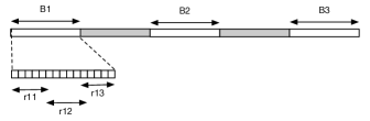
Figure 2: The instance of PSCP when $m=3$, $B=7$. It contains 48 PoIs and 9 sensors. The PoIs are distributed on subsegment $B_{j}$ $(1\leq j\leq 3)$. When the covering range of sensor $s_{i}$ is $\frac{7}{4}\leq r_{i}\leq\frac{7}{2}$ $(1\leq i\leq 9)$, the proper deployment is to deploy 3 sensors to each $B_{j}$.

It is easy to see that $PSCP\in NP$, since it can be checked in polynomial time of $N$ whether the given set of mobile sensors is enough to sweep cover the PoIs or not.

The theorem is proved. ∎

In this process of the above proof, we would find that, considering cooperated strategy or not, PSCP is NP-complete problem.

IV Max-Weight sweep coverage on path problem

We promote an optimization problem for PSCP problem, called Max-PoI Sweep Coverage on Path (MPSCP) problem, which is a special case of Max-Weight sweep coverage on path problem.

defn 6.

(Max-PoI Sweep Coverage on Path Problem) The Max-PoI Sweep Coverage on Path problem is to find the maximum number of PoIs sweep covered on path by the given set of mobile sensors.

In the existing work, there are 2 kinds of optimization problems on point sweep coverage problem proposed. One is Min-sensor Sweep Coverage problem to find minimum number of mobile sensors to sweep cover all the PoIs, the other is Min-idleness sweep coverage problem to minimize maximum time period of the PoIs. However, in applications, resources are always limited. We want to decide whether the given set of mobile sensors can sweep cover the PoIs and if it is not enough, people would like to cover as many PoIs as possible. Max-PoI Sweep Coverage (MPSC) problem is to find the maximum number of PoIs sweep covered by the given mobile sensors. It would maximize utilization efficiency of the given mobile sensors. In theory, MPSC can be used as a decision algorithm for point sweep coverage problem. When the output is $N$, it means all PoIs can be sweep covered by the given set of mobile sensors. We can also use the algorithm for MPSC as a subroutine to fix the Min-sensor sweep coverage problem and the Min-idleness sweep coverage. So it is essential to study MPSC problem.

In this paper, we focus on the point sweep coverage problem on path, so MPSCP would be the our main content. Based on the NPC of PSCP problem, MPSCP problem is a NP-Hard problem.

When we introduce PSCP problem before, we assume the PoIs are on different x-coordinations. Actually, sometimes, some PoIs are on the same x-coordination; or sometimes, PoIs would have different weight depending on their locations’ importance. MPSCP problem would be generalized to its weighted case. We call the weighted case Max-Weight Sweep Coverage on Path (MWSCP) Problem. The object is to find the maximum sum of the weight of PoIs sweep covered, where each of PoIs would have a weight respectively and the weight is allowed to be integer and fractional number. The definition of MWSCP is below.

defn 7.

(Max-Weight Sweep Coverage on Path Problem) Given a set of PoIs on a path and a set of mobile sensors, each of which has a weight respectively, the Max-Weight Sweep Coverage on Path problem is to find the maximum sum of weight of PoIs sweep covered on path by the given set of mobile sensors.

MWSCP is also NP-Hard problem. In the following text, we would fix two kinds of special cases of MWSCP and its general case. We present an optimal algorithm for MWSCP when mobile sensors have uniform velocity and present a $\frac{1}{2}$-approximation algorithm for the case when mobile sensors have constant kinds of velocities. For the general case, we present a $\frac{1}{2\alpha}$-approximation $(\alpha\leavevmode\nobreak\ is\leavevmode\nobreak\ an\leavevmode\nobreak\ integer,\alpha\geq 2)$ algorithm family scheme using rounding method and improve the approximation ratio to $\frac{1}{2}(1-1/e)$ using randomized algorithm.

If the number of PoIs is smaller than or equal to the number of mobile sensors, the problem of MWSCP is trivial. In the following text, we assume the number of PoIs is bigger than the number of mobile sensors, i.e., $N>M$. Static sensors are regarded as special mobile sensors with velocity 0.

IV-A Max-Weight sweep coverage on path with uniform velocity

In this subsection, we show there is a polynomial algorithm for optimal solution for MWSCP when sensors have uniform velocity.

From the paper[17], we know separated strategy is optimal when PoIs on path are sweep covered by mobile sensors with uniform velocity, because when two sensors meet while moving in opposite directions they can “exchange” roles.

lem 8.

Separated strategy is optimal strategy for point sweep coverage on path problem if the given set of mobile sensors have uniform velocity.

Using separated strategy, every sensor has its own covering region. From observation, we find MWSCP using separated strategy problem has the nature of optimal substructure. So we use dynamic programming to get the optimal solution.

Fact 9.

Dynamic programming would be an optimal algorithm to solve MWSCP using separated strategy problem since it has the nature of optimal substructure.

In the case of uniform velocity, we set the uniform velocity of sensors is $v$, then sensors have uniform covering range $r=vT/2$.

Let $OPT(i,j)$ denote the maximum sum of weight of PoIs covered by $i$ sensors from $j^{th}$ PoIs, $n_{j}$ denote the biggest number of PoIs covered by one sensor from $j^{th}$ PoI. $w_{j}$ is the sum of weight of the $n_{j}$ PoIs, i.e., PoIs from $j^{th}$ to $(j+n_{j}-1)^{th}$. The recursive formulation is given below:

$$OPT(i,j)=\\ \begin{array}[]{c}\begin{array}[]{cc}max\left\{\begin{array}[]{c}OPT(i,j+1),\\ OPT(i-1,j+n_{j})+w_{{}_{j}}\end{array}\right\}&\begin{array}[]{c}1\leq i\leq M,\\ 1\leq j<N-1\end{array}\end{array}\end{array}$$

And boundary conditions are

$$OPT(0,j) =0 0\leq j\leq N$$

$$OPT(i,N) =1 1\leq i\leq M$$

The time complexity of the dynamic program is $O(M*N)$ . Since the algorithm is straightforward so we omit it. The dynamic programming algorithm is an optimal algorithm for MWSCP when sensors have uniform velocity.

The PSCP problem when sensors have uniform velocity can also be judged satisfied or not by making the sensors to cover from $1^{th}$ PoI to $N^{th}$ continuously without overlapping.

IV-B Max-Weight sweep coverage on path with constant number of velocities

Now we discuss MWSCP problem when sensors have $K$ different velocities, where $K$ is a constant. In fact, it is not hard to see that the uniform velocity case of MWSCP problem is a special case of MWSCP problem when sensors have constant kinds of velocities. The only difference is that separated strategy is not an optimal strategy any more when $K\geq 2$ and $M\geq 4$[13]. So we use dynamic programming method to find an optimal separated strategy and propose a $\frac{1}{2}$-approximation algorithm for MWSCP problem with constant kinds of velocities considering the difference between separated strategy and cooperated strategy.

Let $m_{i}$ be the number of sensors with velocity $v_{i}$, then $M=\sum\nolimits_{i=1}^{K}m_{i}$. $OPT_{S}(i_{1},i_{2},...,i_{K},j)$ denotes the maximum sum of weight of PoIs covered when there are ${\sum\nolimits_{h=1}^{K}i_{h}}$ sensors to cover the line segment from $j^{th}$ PoI to $N^{th}$ PoI using separated strategy, where $i_{h}$ is the number of sensors with velocity $v_{j}$ $(1\leq h\leq K)$. $n_{ij}$ denotes the maximum number of PoIs covered by a sensor with velocity $v_{i}$ covering from $j^{th}$ PoI and $w_{ij}$ is the sum of weight of the $n_{ij}$ PoIs. The recursive formulation lists below: for $1\leq i_{h}\leq M,1\leq h\leq K,1\leq j\leq N$,

$$OPT_{S}(i_{1},i_{2},...,i_{K},j)=\\ max\left\{\begin{array}[]{c}OPT_{S}(i_{1},i_{2},...,i_{K},j+1),\\ OPT_{S}(i_{1}-1,i_{2},...,i_{K},j+n_{1j})+w_{1j},\\ OPT_{S}(i_{1},i_{2}-1,...,i_{K},j+n_{2j})+w_{2j},\\ ...,\\ OPT_{S}(i_{1},i_{2},...,i_{K}-1,j+n_{Kj})+w_{kj}\end{array}\right\}$$

And boundary conditions are

$$OPT_{S} (0,0,...,0,j)=0$$

$$\qquad\qquad\qquad\hskip 15.00002pt0\leq j\leq N$$

$$OPT_{S} (i_{1},i_{2},...,i_{K},N)=1$$

$$0\leq i_{h}\leq M,1\leq h\leq K,{\sum\nolimits_{h=1}^{K}i_{h}}\geq 1$$

In Algorithm 1, we maintain an array entry $Tr(j)$ for $j=1,...,K$. Each entry $Tr(j)$ is a list of integers. A integer $i$ in the list of entry $Tr(j)$ indicates that $i^{th}$ PoI is the first PoI in the covering region of some sensor with velocity $v_{j}$, whose covering range is $v_{j}T/2$.

Input: The number of sensors $M$, the number of PoIs $N$, sensors’ velocities $V=\{v_{1},v_{2},...,v_{M}\}$, PoIs’ weight $W=\{\omega_{1},\omega_{2},...,\omega_{N}\}$, the number of velocities $K$, sweep period $T$, PoIs’ locations $X=\{x_{1},x_{2},...,x_{N}\}$, an array entry $Tr(i)$ for $1\leq i\leq K$.

Output: The maximum sum of weight of PoIs covered: $O(m_{1},m_{2},...,m_{K},1)$

count the numbers of sensors with different velocities respectively $\{m_{1},m_{2},...,m_{K}\}$;

set $W[K][N]\leftarrow 0$, $Tr[K]\leftarrow 0$;

for  $i\leftarrow 1$ to $K$  do

      for  $j\leftarrow N$ to 1  do

           Let $N[i][j]$ be the biggest number of PoIs covered by one sensor with velocity $v_{i}$ from $j^{th}$ PoI in sweep period $T$, i.e., $w_{ij}$;

           Let $Wt[i][j]$ be the sum of weight of the $N[i][j]$ PoIs covered.;

           end for

          

           end for

          

          set $O[m_{1}+1][m_{2}+1]...[m_{K}+1][N]\leftarrow 0$;;

           initial $O[m_{1}+1][m_{2}+1]...[m_{K}+1][N]$ according to boundary conditions;

          

          for  $j\leftarrow N$ to 1 do

               

               for  $i_{1}\leftarrow 1$ to $m_{1}$  do

                    

                    for  $i_{2}\leftarrow 1$ to $m_{2}$  do

                         

                         for … do

                              

                              for $i_{K}\leftarrow 1$ to $m_{K}$  do

                                    call the recursive formulation to calculate $O(i_{1},i_{2},...,i_{K},j)$;

                                   

                                    end for

                                   

                                    end for

                                   

                                    end for

                                   

                                    end for

                                   

                                    end for

                                   

                                   set $i_{1}=m_{1},i_{2}=m_{2},...,i_{K}=m_{K}$;;

                                    for  $j\leftarrow 1$ to N-1  do

                                        

                                        if $O(i_{1},i_{2},...,i_{K},j)!=O(i_{1},i_{2},...,i_{K},j+1)$  then

                                              for  $h\leftarrow 1$ to $K$  do

                                                   if $i_{h}>0$ $\&\&$ $O(i_{1},i_{2},...,i_{h},...,i_{K},j)==O(i_{1},i_{2},...,i_{h}-1,...,i_{K},j+W[i_{h}][j])+W[i_{h}][j]$  then

                                                        add $j$ to Tr(h); $j-=W[i_{h}][j]$;

                                                        $i_{h}--$;

                                                       

                                                        end if

                                                       

                                                        end for

                                                       

                                                        end if

                                                       

                                                        end for

                                                       

                                                       for  $h\leftarrow 1$ to $K$  do

                                                            

                                                            if  exist $i_{h}!=0$  then

                                                                 

                                                                 add $j$ to Tr(h); break;

                                                                 

                                                                  end if

                                                                 

                                                                  end for

                                                                 

                                                                 for  $1\leq i\leq K$  do

                                                                       place sensors with velocity $v_{i}$ to the locations $Tr(i)$ respectively;

                                                                      

                                                                       end for

                                                                      return $O(m_{1},m_{2},...,m_{K},1)$;

Algorithm 1 MWSCP-K-Velocities

It will take $N*\prod_{i}m_{i}$ time to fix dynamic program in Algorithm 1 and take $N*K$ time to trace back to get the optimal deployment. Note that, $N*\prod_{i}m_{i}\leq N*(M/K)^{K}$, so Algorithm 3 will take $O(N*(M/K)^{K})$ time. Because $K$ is a constant integer, the algorithm is polynomial time algorithm. Now we want to prove that the optimal algorithm for MWSCP using separated strategy is a $\frac{1}{2}$-approximation algorithm for MWSCP. Before that, we prove a more generalized theorem.

thm 10.

A $\beta$-approximation algorithm for MWSCP problem using separated strategy can be turned to be a $\frac{\beta}{2}$-approximation for MWSCP.

Proof:

Let $A$ denote the $\beta$-approximation algorithm for MWSCP problem using separated strategy, and $A_{O}$ denote the optimal algorithm. In resulting deployment of algorithm $A_{O}$, there may be some line segments covered by cooperated strategy and others covered by separated strategy.

Case 1: For the line segments covered by separated strategy in Algorithm $A_{O}$, the sum of weight of PoIs covered in these segments is $OPT_{1}$, which is equal to the sum of weight of PoIs covered by optimal separated strategy. If we sweep cover the same segment with its covering sensors using algorithm $A$, the sum of weight of PoIs covered is $W_{1}\geq\beta*OPT_{1}$.

Case 2: For the line segments covered by cooperated strategy, we assume the optimal sum of weight of PoIs covered is $OPT_{2}$. If we cover the same segment with its covering sensors using optimal separated strategy, we can cover $OPT_{S2}\geq OPT_{2}/2$ PoIs. For example, $l\subseteq L$ is one of the line segments covered by a subset of sensors $S^{\prime}\subseteq S$ with velocities $\left\{v_{1},v_{2},...,v_{n}\right\}$ $(n=|S^{\prime}|)$ using cooperated strategy, in which the sum of weight of PoIs covered is $W_{C}$, $|l|<\sum\nolimits_{i=1}^{n}{v_{i}}$. If we cover $l$ by optimal separated strategy, the covering range of sensors is $|{r}(S^{\prime})|=\sum\nolimits_{i=1}^{n}{{v_{i}}/2}$ and the sum of weight of PoIs covered is $W_{S}$ . If $W_{S}<W_{C}/2$, the uncovered part of segment $l$ whose length is less than $|l|/2$, which can also be covered by $S^{{}^{\prime}}$ containing more weight, then $W_{S}$ is not an optimal solution of separated strategy on segment $l$ . It reduces a contradiction. So $W_{S}\geq W_{C}/2$. It reduces $OPT_{S2}\geq OPT_{2}/2$. Let $W_{2}$ is the sum of weight of PoIs covered by algorithm $A$. We reduce $W_{2}\geq\beta*OPT_{S2}\geq\frac{\text{$\beta$}}{2}*OPT_{2}$.

We get the solution of algorithm $A$ is $W_{1}+W_{2}\geq\frac{\beta}{2}*(OPT_{1}+OPT_{2})$.

The theorem is proved. ∎

thm 11.

Algorithm 3 is an $\frac{1}{2}$-approximation algorithm for MWSCP problem.

Proof:

Algorithm 3 is an optimal dynamic programming algorithm for MWSCP problem using separated strategy. According to Theorem 9, Algorithm 3 is an $\frac{1}{2}$-approximation algorithm for MWSCP problem. ∎

IV-C Max-Weight sweep coverage on path for general cases

In this subsection, we discuss MWSCP for general cases, i.e. when sensors have arbitrary velocities. We use 2 methods to solve the general case of MWSCP problem. One is to use rounding and dynamic programming method, by which we can get a $\frac{1}{2\alpha}$-approximation algorithm scheme, where integer $\alpha\geq 2$. The other is to use randomized method, by which we can get a randomized $\frac{1}{2}$(1-1/e)-approximation algorithm. By conditional expectation method, we can get a deterministic $\frac{1}{2}$(1-1/e)-approximation algorithm by derandomizing the randomized algorithm.

IV-C1 Rounding and dynamic programming method for MWSCP

Given a set of sensors $S$ with velocities $V$, we round the velocities $V$ to $V^{{}^{\prime}}$, make it a new set of sensors input $S^{{}^{\prime}}$. Then we quote Algorithm 1 for sensors $S^{{}^{\prime}}$ to cover the given PoIs. The algorithm 2 is shown below. In the rounding step, let $v_{d}=max\left\{min\leavevmode\nobreak\ d_{min\leavevmode\nobreak\ \alpha},v_{l}\right\}$, where $v_{l}$ denote the lowest velocity except $v_{i}=0$ and $d_{min\leavevmode\nobreak\ \alpha}$ denote the minimum distance between every continuous $\alpha+1$ PoIs. For the sensors in $S$ with velocities lower than $v_{d}$, the velocities will be set to zero. And for the sensors with velocities no lower than $v_{d}$, we set $v_{i}^{{}^{\prime}}=v_{d}*\alpha^{\lfloor log_{\alpha}(v_{i}/v_{d})\rfloor}$ . That is,

$$\begin{cases}v_{i}^{{}^{\prime}}=0&(v_{i}<v_{d},v_{i}\in V)\\ v_{i}^{{}^{\prime}}=v_{d}*2^{\lfloor log_{\alpha}(v_{i}/v_{d})\rfloor}&(v_{i}\geq v_{d},v_{i}\in V)\end{cases}$$

Then the sensors would be rounded to $K=\lceil log_{\alpha}(v_{s}/v_{d})\rceil+1$ groups, where $v_{s}=max\{v_{i}|1\leq i\leq M\}$.

Input: The number of sensors $M$, the number of PoIs $N$, sensors’ velocities $V=\{v_{1},v_{2},...,v_{M}\}$, PoIs’ weight $W=\{\omega_{1},\omega_{2},...,\omega_{N}\}$, sweep period $T$, PoIs’ locations $X=\{x_{1},x_{2},...,x_{N}\}$.

Output: The maximum sum of weight of PoIs sweep covered.

for  $i\leftarrow 1$ to $N-2$  do

      $d_{i,i+2}=x_{i+2}-x_{i}$;

      end for

     

     set $v_{d}=max\{min\{v_{i}|v_{i}\neq 0,1\leq i\leq M\},min\{d_{i,i+2}|1\leq i\leq N-2\}\}$;

     

     set $v_{s}=max\{v_{i}|1\leq i\leq M\}$;

     

     set $m=\lceil log_{\alpha}(v_{s}/v_{d})\rceil$;

     

     for  $i\leftarrow 1$ to $M$  do

          

          if  $v_{i}\geq v_{d}$  then

                // For the sensors with velocities no less than $v_{d}$;

                set $\sigma=\lfloor log_{\alpha}(v_{i}/v_{d})\rfloor$ ;

                set $v_{i}^{{}^{\prime}}=\alpha^{\sigma}*v_{d}$ ;

                else

                     //For the sensors with velocities less than $v_{d}$;

                     $v<v_{d}$;

                     $v_{i}^{{}^{\prime}}=0$;

                    

                     end if

                    

                     end for

                    

                    set $V^{{}^{\prime}}=\{v_{i}^{{}^{\prime}}|1\leq i\leq M\}$, $K=m+1$;

                    

                    initial an entry array $Tr(i)$ for $1\leq i\leq K$ ;

                    

                    apply algorithm 1 to new input ($M$ sensors, $N$ PoIs, sensors’ velocities $V^{{}^{\prime}}$, PoIs’ weight $W$, the number of kinds of velocities $K$, sweep period $T$, PoIs’ locations $X$, $Tr(i)$ for $1\leq i\leq K$);

                    

                    place the sensors with velocities $v_{i}$ to the locations we get from algorithm 1 for the sensors with velocity $v_{i}^{{}^{\prime}}$ ;

                    

return $A_{1}(V^{{}^{\prime}})$

Algorithm 2 MWSCP-General-Cases

Now we prove Algorithm 2 is a $\frac{1}{2\alpha}$-approximation algorithm scheme.

thm 12.

Algorithm 2 is a $\frac{1}{2\alpha}$-approximation algorithm.

Proof:

Given a set of sensors $S$ with velocities $V$, we can get a new set of sensors $S^{{}^{\prime}}$ with rounded velocities $V^{{}^{\prime}}$ like algorithm 2. We assume $A_{1}(S)$ is the optimal separated strategy for $S$. In $A_{1}(S)$ for every sensors $s_{i}\in S$, there is a covering region $R(s_{i})$. For every sensor $s_{i}$ with velocity $v_{i}$ not lower than $v_{d}$, we set $v_{i}^{{}^{\prime}}=v_{d}*\alpha^{\lfloor log_{\alpha}(v_{i}/v_{d})\rfloor}$ , then $v_{i}^{{}^{\prime}}\leq v_{i}\leq\alpha v_{i}^{{}^{\prime}}$. The region $R(s_{i})$ can be covered by $\alpha$ copies of the sensor $s_{i}^{{}^{\prime}}$ with velocity $v_{i}^{{}^{\prime}}$ for each $s_{i}\in S$. According to Pigeonhole principle, there must be a covering region $R^{{}^{\prime}}(s_{i}^{{}^{\prime}})$ covered by one sensor with velocity $v_{i}^{{}^{\prime}}$ having the sum of weight no less than $w(s_{i})/\alpha$, where $\omega(s_{i})$ is the sum of weight of PoIs on range $R(s_{i})$. For each sensor $s_{i}\in S$ with velocity lower than $v_{d}$, note that the covering region $R(s_{i})$ can not cover more than $\alpha$ PoIs, so $R(s_{i})$ can be also covered by $\alpha$ copies of sensor with velocity 0. If we design a new algorithm, let sensor $s_{i}^{{}^{\prime}}\in S^{{}^{\prime}}$ cover the the covering region $R^{{}^{\prime}}(s_{i}^{{}^{\prime}})$ with no less than $w(s_{i})/\alpha$ weight when $v_{i}\geq v_{d}$, otherwise, cover the PoI with most weight in $R(s_{i})$ when $v_{i}<v_{d}$, then we can get a separated deployment for $S^{{}^{\prime}}$, which can obtain the sum of weight no smaller than $A_{1}(S)/\alpha$.

Because $A_{1}(S^{{}^{\prime}})$ is an optimal separated strategy for $S^{{}^{\prime}}$, $A_{1}(S^{{}^{\prime}})$ can at least get the same weight as the deployment above.

According to theorem 9, That Algorithm 4 is a $\frac{1}{2\alpha}$-approximation algorithm is proved. ∎

Note that $\alpha$ is an integer and $\alpha\geq 2$. Some counterexamples show that $\alpha$ can not be fractional number. So we can get the best performance guarantee is $\frac{1}{4}$-approximation by Algorithm 2. Algorithm 2 quote algorithm 1, so the time complexity is $O(N*(M/K)^{K})$ where $K=\lceil log_{\alpha}(v_{s}/v_{d})\rceil+1$. $\alpha$ is a tradeoff between time complexity and performance guarantee. In most cases, the maximum velocity is constant times of minimum nonzero velocity, so $K$ is a constant to make the time complexity of Algorithm 2 is acceptable.

.

IV-C2 Randomized rounding algorithm for MWSCP

Rounding and dynamic programming method gives a $\frac{1}{2\alpha}$-approximation algorithm, where integer $\alpha\geq 2$. Its best performance guarantee is $\frac{1}{4}$-approximation. In this subsection, we use randomized algorithm to analyze MWSCP problem and get an approximation algorithm with better performance guarantee, $\frac{1}{2}(1-1/e)\approx 0.31606$. Besides, no matter the difference between the maximum velocity and the minimum velocity, this algorithm takes polynomial time complexity.

Actually, we still analyze MWSCP problem using separated strategy to get a $(1-1/e)$-approximation algorithm at first, and then get a $\frac{1}{2}(1-1/e)$-approximation algorithm for MWSCP problem without eliminating the cooperated strategy. We use the following integer programming formulation to denote MWSCP using separated strategy problem, where the variable $z_{l}$ indicates whether the $l^{th}$ PoI is covered, the variable $x_{ij}$ indicates whether sensor i sweep cover from $j^{th}$ PoI, and $S_{ij}$ indicates the set of PoIs covered if sensor i sweep covered from $j^{th}$ PoI. $x_{ij}=1$ means the PoIs in $S_{ij}$ are sweep covered. Then the constraint (4) must hold for each PoI $z_{l}$ since at least one set $S_{ij}$ containing $z_{l}$ is included in solution when $z_{l}=1$ and no set containing $z_{l}$ is included otherwise. The constraint (5) means one sensor can be only used once.

$$max\sum_{l=1}^{n}\omega_{l}z_{l}$$

$$s.t. \sum_{(i,j):l\in S_{ij}}x_{ij}\geq z_{l} \forall l\in N$$ (4)

$$\sum_{j}x_{ij}\leq 1 \forall i\in M$$

$$x_{ij}\in\{0,1\} \forall i\in M,j\in N$$

$$z_{l}\in\{0,1\} \forall l\in N$$

Then we get the following linear programming relaxation from the integer program above by replacing the constraints $x_{ij}\in\{0,1\}$ and $z_{l}\in\{0,1\}$ with $0\leq x_{ij}\leq 1$ and $z_{l}\leq 1$ .

$$max\sum_{l=1}^{n}\omega_{l}z_{l}$$

$$s.t. \sum_{(i,j):l\in S_{ij}}x_{ij}\geq z_{l} \forall l\in N$$

$$\sum_{j}x_{ij}\leq 1 \forall i\in M$$

$$0\leq x_{ij}\leq 1 \forall i\in M,j\in N$$

$$z_{l}\leq 1 \forall l\in N$$

Let $(x^{*},z^{*})$ is the optimal solution to the linear program. We use randomized rounding method to analyze MWSCP problem by making sensor i to sweep cover from $j^{th}$ PoI with probability $x_{ij}^{*}$ independently. Then we can get a $(1-1/e)$-approximation randomized algorithm for MWSCP using separated strategy problem.

Input: The number of sensors $M$, the number of PoIs $N$, sensors’ velocities $V=\{v_{1},v_{2},...,v_{M}\}$, PoIs’ weight $W=\{\omega_{1},\omega_{2},...,\omega_{N}\}$, sweep period $T$, PoIs’ locations $X=\{x_{1},x_{2},...,x_{N}\}$.

Output: The maximum sum of weight of PoIs covered

compute an optimal solution $(y^{*},z^{*})$ to the linear program relaxation.

for  $i\leftarrow 1$ to $M$  do

      make sensor $i$ cover from $j^{th}$ PoI independently at random with probability $x_{ij}^{*}$ .;

     

      end for

     

     return

Algorithm 3 Randomized rounding algorithm for MWSCP

thm 13.

Algorithm 3 is a randomized $\frac{1}{2}$(1-1/e)-approximation algorithm for MWSCP.

Proof.

The fractional value $x_{ij}^{*}$ is interpreted as the probability that $S_{ij}$ is chosen. The proof is similar to the proof of theorem 5.10 in [williamson2011design]. Then we see the probability that $z_{l}$ is not covered is

$$Pr[z_{l}\leavevmode\nobreak\ is\leavevmode\nobreak\ not\leavevmode\nobreak\ coverd] = \prod_{(i,j):l\in S_{ij}}(1-x_{ij}^{*})$$

$$\leq [{\frac{1}{n_{l}}\sum_{(i,j):l\in S_{ij}}(1-x_{ij}^{*})}]^{n_{l}}$$

$$\leq (1-\frac{\sum x_{ij}^{*}}{n_{l}})^{n_{l}}$$

$$\leq (1-\frac{z_{l}^{*}}{n_{l}})^{n_{l}}$$

Where $n_{l}$ indicates the number of sets in which $z_{l}$ is included and the last inequality follows from the constraint (6).

When $n_{l}\geq 1$, $f(z_{l}^{*})=1-(1-\frac{z_{l}^{*}}{n_{l}})^{n_{l}}$ is concave. So the probability that $z_{l}$ is covered is

$$Pr[z_{l}\leavevmode\nobreak\ is\leavevmode\nobreak\ covered] \geq 1-(1-\frac{z_{l}^{*}}{n_{l}})^{n_{l}}$$

$$\geq [{1-(1-\frac{1}{n_{l}})^{n_{l}}}]z_{l}^{*}$$

Let W be a random variable that is equal to the total weight of the covered PoIs. let $Y_{l}$ is a random variable such that $Y_{l}$ is 1 if $z_{l}$ is covered and 0 otherwise. We know that

$$E[W] = \sum_{l=1}^{n}\omega_{l}E[Y_{l}]$$

$$= \sum_{l=1}^{n}\omega_{l}Pr(z_{l}\leavevmode\nobreak\ is\leavevmode\nobreak\ covered)$$

$$\geq \sum_{l=1}^{n}\omega_{l}z_{l}^{*}[1-(1-\frac{1}{n_{l}})^{n_{l}}]$$

$$\geq min_{k\geq 1}[1-(1-\frac{1}{k})^{k}]\sum_{l=1}^{n}\omega_{l}z_{l}^{*}$$

$$\geq (1-\frac{1}{e})OPT$$

Now we prove that we can get randomized $(1-1/e)$-approximation algorithm for MWSCP using separated strategy problem by randomized rounding technique. According to theorem 9, Algorithm 4 is $\frac{1}{2}(1-1/e)$-approximation algorithm for MWSCP. ∎

By the method of conditional expectations, we can obtain a deterministic algorithm, Algorithm 4, that has the same performance guarantee as the randomized one. So the algorithm 4 is a deterministic $\frac{1}{2}(1-1/e)$approximation algorithm. Since it takes polynomial time of input to solve the linear programming formulation, denoted as $p(N)$ and $M*N$ linear programming formulations are needed to be solved in the derandomized algorithm. The algorithm 4 is a polynomial algorithm and its time complexity is $O(M*N*p(N))$.

Input: The number of sensors $M$, the number of PoIs $N$, sensors’ velocities $V=\{v_{1},v_{2},...,v_{M}\}$, PoIs’ weight $W=\{\omega_{1},\omega_{2},...,\omega_{N}\}$, sweep period $T$, PoIs’ locations $X=\{x_{1},x_{2},...,x_{N}\}$.

Output: The maximum sum of weight of PoIs covered.

for  $i\leftarrow 1$ to $M$  do

      set $j_{i}=argmax_{j\in N}E(W|x_{1j_{1}}=1,...,x_{(i-1)j_{(i-1)}}=1,x_{ij}=1)$ .;

     

      end for

     

     for  $i\leftarrow 1$ to $M$  do

           make sensor $i$ to cover from $j_{i}^{th}$ PoI. ;

          

           end for

          

          $St=\cup_{i}S_{ij_{i}}$;

          

          $\omega t=\sum_{z_{l}\in St}\omega_{l}$;

          

return $\omega t$

Algorithm 4 Deterministic version for MWSCP

Note that in the algorithm 4,

$$E[W|x_{1j_{1}}=1,...,x_{(i-1)j_{(i-1)}}=1,x_{ij}=1]$$

$$= \sum_{l\in N}\omega_{l}Pr[z_{l}|x_{1j_{1}}=1,...,x_{(i-1)j_{(i-1)}}=1,x_{ij}=1]$$

where $x_{ij_{i}}=1$ means that $j_{i}$ is the final optimal starting location of sensor $i$.

Randomized method usually gets better approximation ratio than $\frac{1}{2}(1-1/e)$ in practice .

V Conclusion

There are many applications of sweep coverage on path, such as forest patrol and intruder detection. In this paper, we first study the problem of point sweep coverage on path and prove it is NP-Complete. We also define its variant, the Max-Weight sweep coverage on path problem, which are NP-Hard. For MWSCP, we propose an optimal algorithm for the case that sensors have uniform velocity and a $\frac{1}{2}$-approximation algorithm for sensors with constant number of velocities. For the general case of MWSCP, we propose two algorithms. One is a $\frac{1}{2\alpha}$-approximation algorithm family scheme, where integer $\alpha\geq 2$. The other is a $\frac{1}{2}(1-1/e)$-approximation algorithm. It is interesting to study Max-Weight sweep coverage problem in other kinds of graphs, e.g., trees, Eulerian graphs and so on. That is what we are about to study.

References

- [1] Zhiyin Chen, Xudong Zhu, Xiaofeng Gao, Fan Wu, Jian Gu, and Guihai Chen. Efficient scheduling strategies for mobile sensors in sweep coverage problem. In Sensing, Communication, and Networking (SECON), 2016 13th Annual IEEE International Conference on, pages 1–4. IEEE, 2016.
- [2] Weifang Cheng, Mo Li, Kebin Liu, Yunhao Liu, Xiangyang Li, and Xiangke Liao. Sweep coverage with mobile sensors. In Parallel and Distributed Processing, 2008. IPDPS 2008. IEEE International Symposium on, pages 1–9. IEEE, 2008.
- [3] Andrew Collins, Jurek Czyzowicz, Leszek Gasieniec, Adrian Kosowski, Evangelos Kranakis, Danny Krizanc, Russell Martin, and Oscar Morales Ponce. Optimal patrolling of fragmented boundaries. In Proceedings of the twenty-fifth annual ACM symposium on Parallelism in algorithms and architectures, pages 241–250. ACM, 2013.
- [4] Jurek Czyzowicz, Leszek Ga̧sieniec, Adrian Kosowski, and Evangelos Kranakis. Boundary patrolling by mobile agents with distinct maximal speeds. In European Symposium on Algorithms, pages 701–712. Springer, 2011.
- [5] Junzhao Du, Yawei Li, Hui Liu, and Kewei Sha. On sweep coverage with minimum mobile sensors. In Parallel and Distributed Systems (ICPADS), 2010 IEEE 16th International Conference on, pages 283–290. IEEE, 2010.
- [6] Adrian Dumitrescu, Anirban Ghosh, and Csaba D Tóth. On fence patrolling by mobile agents. arXiv preprint arXiv:1401.6070, 2014.
- [7] Michael R Gary and David S Johnson. Computers and intractability: A guide to the theory of np-completeness, 1979.
- [8] Barun Gorain and Partha Sarathi Mandal. Point and area sweep coverage in wireless sensor networks. In Modeling & Optimization in Mobile, Ad Hoc & Wireless Networks (WiOpt), 2013 11th International Symposium on, pages 140–145. IEEE, 2013.
- [9] Barun Gorain and Partha Sarathi Mandal. Approximation algorithms for sweep coverage in wireless sensor networks. Journal of Parallel and Distributed Computing, 74(8):2699–2707, 2014.
- [10] Barun Gorain and Partha Sarathi Mandal. Line sweep coverage in wireless sensor networks. In 2014 Sixth International Conference on Communication Systems and Networks (COMSNETS), pages 1–6. IEEE, 2014.
- [11] Barun Gorain and Partha Sarathi Mandal. Approximation algorithm for sweep coverage on graph. Information Processing Letters, 115(9):712–718, 2015.
- [12] Barun Gorain and Partha Sarathi Mandal. Solving energy issues for sweep coverage in wireless sensor networks. Discrete Applied Mathematics, 2016.
- [13] Akitoshi Kawamura and Yusuke Kobayashi. Fence patrolling by mobile agents with distinct speeds. Distributed Computing, 28(2):147–154, 2015.
- [14] Akitoshi Kawamura and Makoto Soejima. Simple strategies versus optimal schedules in multi-agent patrolling. In International Conference on Algorithms and Complexity, pages 261–273. Springer, 2015.
- [15] Linghe Kong, Mingchen Zhao, Xiao-Yang Liu, Jialiang Lu, Yunhuai Liu, Min-You Wu, and Wei Shu. Surface coverage in sensor networks. IEEE Transactions on Parallel and Distributed Systems, 25(1):234–243, 2014.
- [16] Shuangjuan Li and Hong Shen. Minimizing the maximum sensor movement for barrier coverage in the plane. In 2015 IEEE Conference on Computer Communications (INFOCOM), pages 244–252. IEEE, 2015.
- [17] Fabio Pasqualetti, Antonio Franchi, and Francesco Bullo. On cooperative patrolling: Optimal trajectories, complexity analysis, and approximation algorithms. IEEE Transactions on Robotics, 28(3):592–606, 2012.
- [18] Soumyadip Sengupta, Swagatam Das, MD Nasir, and Bijaya K Panigrahi. Multi-objective node deployment in wsns: In search of an optimal trade-off among coverage, lifetime, energy consumption, and connectivity. Engineering Applications of Artificial Intelligence, 26(1):405–416, 2013.
- [19] Zuoming Yu, Jin Teng, Xiaole Bai, Dong Xuan, and Weijia Jia. Connected coverage in wireless networks with directional antennas. ACM Transactions on Sensor Networks (TOSN), 10(3):51, 2014.