Optimal Photon blockade on the maximal atomic coherence

Abstract

There is generally no obvious evidence in any direct relation between photon blockade and atomic coherence. Here instead of only illustrating the photon statistics, we show an interesting relation between the steady-state photon blockade and the atomic coherence by designing a weakly driven cavity QED system with a two-level atom trapped. It is shown for the first time that the maximal atomic coherence has a perfect correspondence with the optimal photon blockade. The negative effects of the strong dissipations on photon statistics, atomic coherence and their correspondence are also addressed. The numerical simulation is also given to support all of our results.

I Introduction

Photon statistics including photon blockade and photon-induced tunneling have attracted extensive attention in the past years. They result from the nonlinearity of the cavity field blocka ; hui and as the typical nonlinear quantum optical effects, are necessary ingredients for prospective developments in quantum information processing optimal . Photon blockade indicates the ability to control the nonlinear response of a system by the injection of single photon blocka , while the phenomenon of photon-induced tunneling is that the system increases the entering probability of subsequent photons hui . These typical features have been theoretically predicted and experimentally observed in many physical systems such as opto-mechanical setups, feed-back control system, super-conducting circuit and so on Rabl ; Nunnenkamp ; 87 ; liao ; yulong ; Hoffman ; Liu ; Winger ; Kimble ; 77 ; Verger . Cavity quantum electrodynamics (CQED) is an important medium to study the atom-photon interactions coherent ; kai ; Rempe ; arka1 ; arka2 ; tianlin . The optical nonlinearity in such a system arises from the discrete energy level structure of the atom, so it has an important application in the photon statistics Kimble ; 77 ; lun ; arka ; zy .

Recently, quantum coherence as an essential ingredient of the quantum world has been widely studied Adesso1 ; Adesso ; Adesso4 ; DD ; yd ; Streltsov ; Marvian . It is at the root of a number of intriguing phenomena of wide-ranging impact in quantum optics Albrecht ; Glauber ; M , where decoherence due to the interaction with an environment is a crucial issue that is of fundamental interest. Quantum coherence which can also been understood via the theory of physical resource plenio1 ; quant has attracted increasing interests in many aspects Yu1 ; yao ; fan ; Lostaglio ; Monras such as hot systems hot , many-body systems Barontini ; Barreiro , biological system plenio1 ; plenio2 ; Ishizaki ; Castro , low-temperature thermodynamics Lostaglio ; berg ; Adesso3 , solid-state physics Lambert , optimization of squeezed light squ and so on. In particular, one of the intriguing aspects of quantum coherence is that the atomic coherence has the ability to enhance the efficiencies of nonlinear optical processes xm ; Harris ; Ebert ; joo . Since the photon blockade requires the strong optical nonlinearity, is there a clear quantitative relation between the atomic coherence and photon blockade in a cavity-atom interaction system? Intuitively, there is no obvious evidence in the relation between the photon blockade and atomic coherence. So we will turn to another weak question whether we can find a physical model that can show the relation between quantum blockade and atomic coherence?

In the present work, we design a weakly driven cavity QED system with a two-level atom trapped and study the relation between the steady-state photon blockade and the atomic coherence. Our interest is not to only illustrate the photon statistics, but to reveal the particularly interesting correspondence between the photon blockade and the coherence of the atom in the steady state. As our main result, we find that in the case of steady state, the atomic coherence has a perfectly consistence with the photon blockade effect. That is, the maximal atomic coherence just corresponds to the optimal photon blockade, but the local maximal bunching points which subject to a two-photon excitation process or a quasi-dark-state process corresponds to nearly vanishing coherence. In addition, we have also shown that once the dissipations of the system become relatively strong, the atomic coherence and the photon anti-bunching effect will be reduced, meanwhile there appears a deviation in the correspondence between atomic coherence and photon blockade because of the increasing widths of the energy levels. The remaining of this paper is organized as follows. In Sec. 2, we briefly describe our model. In Sec. 3, we discuss the mechanism of photon -induced tunneling and photon blockade by the analytical method. In Sec. 4, we study the atomic coherence and present the correspondence relation between coherence and different statistics, whilst a numerical simulation based on the master equation is also given to support our analytic treatment. Finally, we draw our conclusion and give some discussions.

II The physical model

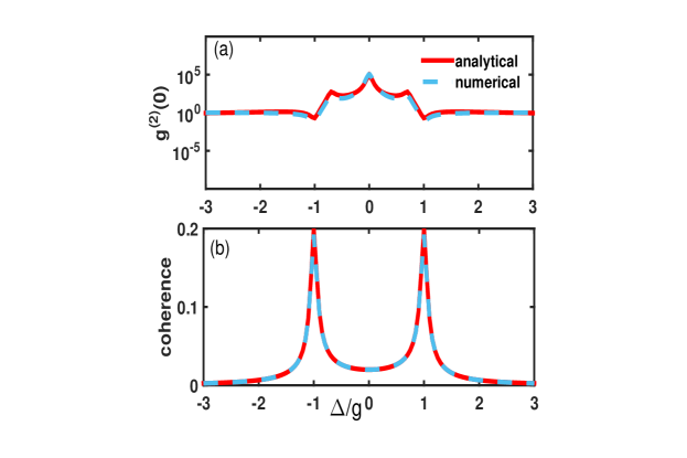
Figure 1: (color online). The equal-time second-order function $g^{(2)}(0)$ and the coherence of atom vs the detuning $\Delta$, respectively. The red curves are analytical results and the green curves are numerical results of the quantum master equation. We take $\gamma/g=0.05,$ $\kappa/g=0.05$, $\eta/g=0.01$.

The system we studied here consists of a single atom (with ground state $\left|g\right\rangle$ and excited state $\left|e\right\rangle$) coupled to a cavity mode and the cavity is weakly driven by a laser with the frequency denoted by $\omega_{L}$ and the Rabi frequency denoted by $\eta$. The coupled system is well governed by the Hamiltonian $H$ (we set $\hbar=1$ hereafter)

$$H = \omega_{a}a^{{\dagger}}a+\omega_{e}\sigma^{+}\sigma^{-}+g(\sigma^{+}a+a^{{\dagger}}\sigma^{-})$$

$$+\eta\left(a^{{\dagger}}e^{-i\omega_{L}t}+ae^{i\omega_{L}t}\right),$$

where $a$ and $\sigma^{-}=\left|g\right\rangle\left\langle e\right|$ are the annihilation and lowering operators for the cavity mode and the atom, respectively and $\omega_{e}$ is the frequency of atomic transition from ground state $\left|g\right\rangle$ to excited state $\left|e\right\rangle$ and $\omega_{a}$ is the cavity resonance frequency. In addition, we set the coupling coefficient between the atom and the cavity mode to be $g$. In the frame rotated at the laser frequency $\omega_{L}$, the Hamiltonian (II) can be rewritten as

$$H = \Delta_{a}a^{{\dagger}}a+\delta\sigma^{+}\sigma^{-}+g(\sigma^{+}a+a^{{\dagger}}\sigma^{-})$$ (2)

$$+\eta\left(a^{{\dagger}}+a\right),$$

with the laser detuning from the cavity mode $\Delta_{a}=\omega_{a}-\omega_{L}$ and $\allowbreak\delta=\omega_{e}-\omega_{L}$ corresponding to the laser detuning from the atom.

For simplicity, we assume that the cavity is resonant with the atom, i.e., $\omega_{a}=\omega_{c}$ and $\Delta_{a}=\delta=\Delta$. Since the system is driven weakly, only few photons can be excited. Thus we can only focus on the few-photon subspace. In this regime, energy eigenstates are in two-level manifolds. So the eigenenergies and eigenstates of the Hamiltonian without driving can be given by

$$E_{n\pm} = n\Delta\pm g\sqrt{n},$$

$$\left|n,-\right\rangle = \frac{1}{\sqrt{2}}(\left|n,g\right\rangle-\left|n-1,e\right\rangle),$$

$$\left|n,+\right\rangle = \frac{1}{\sqrt{2}}(\left|n,g\right\rangle+\left|n-1,e\right\rangle),$$ (3)

where $n$ is the number of energy quanta in the CQED system (in the weak driving regime, we can safely cut off the photon number to 2 ) which distinguishes the different eigenstates. One can easily find the eigenenergies in the manifolds depend on the coupling $g$ (the equivalent coupling rate is $g\sqrt{n}$). The nonlinearity in the coupling between the atom and cavity gives rise to energy level structure which can exhibit different photon statistics behaviors due to the splitting of the eigenenergy jc .

When the environmental effect is taken into account in the current system, there are two mechanisms for energy dissipation: cavity decay and spontaneous emission of the atom. We assume zero temperature reservoirs, the corresponding master equation can be given in the following Lindblad form

$$\dot{\rho} = -i[H,\rho]+\kappa(2a\rho a^{\dagger}-a^{\dagger}a\rho-\rho a^{\dagger}a)$$ (4)

$$+ \gamma(2\sigma^{-}\rho\sigma^{+}-\sigma^{+}\sigma^{-}\rho-\rho\sigma^{+}\sigma^{-}),$$

where $H$ is the system’s original Hamiltonian as given by Eq. (2), $\rho$ is the density operator for the atom-cavity system, $\kappa$ is the field decay rate for the cavity mode, $\gamma$ is the atomic spontaneous emission rate. In general, for a full quantum mechanical treatment of the system, we can compute the numerical solutions to the master equation Eq. (4) using truncated number state bases for the cavity mode 77 . Here, we restrict ourselves in the subspace spanned by the basis $\{\left|n,g\right\rangle,$ $\left|n-1,e\right\rangle\},$ hence the formal solution of $\rho$ can be gotten. Once $\rho$ is given, any physical quantity of the system can be obtained.

III The photon statistics

As mentioned at the beginning, the signatures of the photon behaviors can be detected through photon statistics measurement arka , which can be characterized by the normalized the equal-time correlation function, which is defined for stationary state scully

$$g^{(2)}(0)=\frac{\left\langle a^{\dagger}a^{\dagger}aa\right\rangle}{\langle a^{\dagger}a\rangle^{2}}=\frac{Tr[\rho_{s}a^{\dagger 2}a^{2}]}{[Tr(\rho_{s}a^{\dagger}a)]^{2}},$$ (5)

where $a$ is the annihilation operator for the cavity mode, the $\rho_{s}$ is the steady-state density matrix of the composite system which can be obtained by employing a numerical way to solving the master equation in Eq. (5) tan1 . The photon blockade which means the system ’blocks’ the absorption of a second photon with the same energy and large probability. The limit $g^{(2)}(0)\rightarrow 0$ means the perfect photon blockade in which two photons never occupy the cavity at the same time. On the contrary, when $g^{(2)}(0)>1$, it means photons inside the cavity enhance the resonantly entering probability of subsequent photons li1 ; li2 ; lang .

In order to gain more insight into the physics, we first take an analytic (but approximate) method to calculate the second-order correlation function with the help of the wave function amplitude approach by employing the Schrödinger equation open

$$i\frac{d\left|\Psi\right\rangle}{dt}=H_{eff}\left|\Psi\right\rangle.$$ (6)

Considering the effects of the two channels (the leakage of the cavity $\kappa$, the spontaneous emission $\gamma$ of the atom) , we phenomenologically add the relevant damping contributions to Eq. (2). Thus the effective Hamiltonian can be rewritten as

$$H_{eff}=H-\frac{i}{2}(\kappa a^{\dagger}a+\gamma\sigma^{+}\sigma^{-}).$$ (7)

Analogously to the above statements, we can omit the probability for three or more photons due to the weak driving. This makes it easy to evaluate following analytical expression. In this case, we can suppose that the state of the system can be expressed as fliuds ; steady1 ; Carmichael

$$\left|\Psi\right\rangle = C_{0g}\left|0,g\right\rangle+C_{1g}\left|1,g\right\rangle+C_{0e}\left|0,e\right\rangle$$ (8)

$$+C_{2g}\left|2,g\right\rangle+C_{1e}\left|1,e\right\rangle.$$

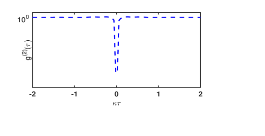
Figure 2: (color online). The evolution of finite time delay correlation function $\ g^{(2)}(\tau)$ of the cavity mode by numerical simulation the master equation. $\ g^{(2)}(\tau)$ exhibits photon antibunching $g^{(2)}(0)\prec g^{(2)}(\tau)$, and sub-Poissonian photon statistics $g^{(2)}(0)\prec 1$. Here, $\gamma/\kappa$=1, $\Delta/\kappa=\delta/\kappa=-20,$ $g/\kappa=20$ .

Based on the definition of $g^{(2)}(0)$, i.e.,

$$g^{(2)}(0)=\frac{\sum_{n}n(n-1)p_{n}}{(\sum_{n}np_{n})^{2}}=\frac{2p_{2}}{(p_{1}+2p_{2})^{2}},$$ (9)

where $p_{n}=$ $\left|C_{n}\right|^{2}$ represents the probability with $n$ photons and $p_{1}=\left|\bar{C}_{1g}\right|^{2},p_{2}=\left|\bar{C}_{2g}\right|^{2}$, one find that $g^{(2)}(0)$ can be obtained so long as one can solve $C_{n}$ given in Eq. (8). To do so, we substitute $\left|\Psi\right\rangle$ into Eq. (6) and arrive at the following dynamical equations

$$\dot{C}_{1g} = -(\kappa/2+i\Delta_{a})C_{1g}-i\eta C_{0g}-igC_{0e}-\sqrt{2}i\eta C_{2g},$$

$$\dot{C}_{0e} = -(\gamma/2+i\delta)C_{0e}-igC_{1g}-i\eta C_{1e},$$

$$\dot{C}_{2g} = -2(\kappa/2+i\Delta_{a})C_{2g}-\sqrt{2}igC_{1e},$$ (10)

$$\dot{C}_{1e} = -(\kappa/2+\gamma/2+i\delta+i\Delta_{a})C_{1e}-\sqrt{2}igC_{2g}-i\eta C_{1e}.$$

Let the initial state of the system be $\left|0,g\right\rangle$. Considering the limit of the weakly driving field again, we can get $\bar{C}_{0g}$ $\rightarrow$ $1$, and Eq. (10) are closed. Thus, Eq. (10) can be easily solved. In the following, we will only consider the question in the steady-state case. In addition, the steady-state solution of Eq. (10) can be analytically obtained, but the precise form are quite cumbersome, so we further neglect the high-order terms of $\eta$ (weak driving) in Eq. (10). Under these conditions, we can get the steady-state solution of Eq. (10) as follows.

$$\bar{C}_{1g}=-\frac{i\eta\alpha}{g^{2}+\alpha\beta},$$ (11)

$$\bar{C}_{0e}=-\frac{g\eta}{g^{2}+\alpha\beta},$$ (12)

$$\bar{C}_{2g}=-\frac{\eta^{2}[g^{2}-\alpha^{2}-\alpha\beta]}{\sqrt{2}(g^{2}+\alpha\beta)(g^{2}+\beta^{2}+\alpha\beta)},$$ (13)

$$\bar{C}_{1e}=\frac{ig^{2}\eta^{2}(\alpha+\beta)}{(g^{2}+\alpha\beta)(g^{2}+\beta^{2}+\alpha\beta)},$$ (14)

with $\alpha=(\gamma/2+i\delta),$ $\beta=(\kappa/2+i\Delta_{a}).$ In the weak-driving case, we can easily get $p_{1}\gg p_{2}$, then the equal-time second-order correlation function can be simplified as $g^{(2)}(0)\approx\frac{2p_{2}}{(p_{1})^{2}}$. It can be further written by

$$g^{(2)}(0)\approx\frac{xy}{z},$$ (15)

where $x:=(g^{2}+\alpha\beta)(g^{2}+\alpha^{\ast}\beta^{\ast}),$ $y:=(g^{2}-\alpha(\alpha+\beta))(g^{2}-\alpha^{\ast}(\alpha^{\ast}+\beta^{\ast})),$ $z:=\alpha^{2}\alpha^{\ast 2}(g^{2}+\beta(\alpha+\beta))(g^{2}+\beta^{\ast}(\alpha^{\ast}+\beta^{\ast})).$

In Fig. 1 (a), we plot $g^{(2)}(0)$ with the detuning $\Delta$ to illustrate the behaviors of photon antibunching and bunching in the case of weak dissipations and driving (here we let $\Delta_{a}=\delta=$ $\Delta$). In this figure, $\Delta=\{\pm g,\pm\sqrt{2}g/2\}$ corresponds to the photon sub-Poissonian and super-Poissonian, respectively. In the blockade regime, the successful blocking of the second photon depends on how well the first photon is coupled to the CQED system arka1 . The quantum signatures can also be manifested by a finite time delay second-order function $g^{(2)}(\tau),$ Based on the second-order correlation function, one can know whether the photon anti-bunching happened or not. The photon antibunching can be demonstrated by a rise of $g^{(2)}(\tau)$ with $\tau$ increasing from 0 to larger values while $g^{(2)}(0)\prec g^{(2)}(\tau)$ pp ; lang . Since reaching $g^{(2)}(\tau)\succ$ $g^{(2)}(0),$ it violates Cauchy-Shwarz inequality and is a nonclassical effect. As shown in Fig. 2, photon antibunching can be observed, $g^{(2)}(0)$ is at a minimum and $g^{(2)}(\tau)$ rise for increasing $\tau.$

IV Atomic coherence and photon statistics

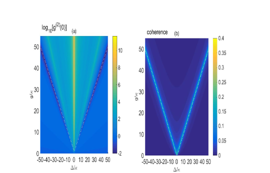
Figure 3: (color online). (a) Logarithmic plot the equal-time second-order function $g^{(2)}(0)$ in (a) as a function of the cavity-atom coupling rate $g$ and detuning $\Delta$. (b) The plot of the atomic coherence varying with $g$ and $\Delta$. The optimal photon anti-bunching and the maximal coherence are illustrated by the white-dashed line respectively in (a) and (b) which corresponds to $\Delta^{2}=g^{2}$. Here, $\gamma/\kappa$=0.5, $\eta/\kappa=0.1$.

In this section, we will give a detailed investigation of the atom’s coherence. It has been shown that the off-diagonal elements of $\rho$ characterize interference. They are usually called as coherence with respect to the basis in which $\rho$ is written wall ; Yu ; ot ; ann . The coherence can be measured by Yu

$$C(\rho)=\left\|\rho-\sigma^{\ast}\right\|_{1}=\sum\limits_{i\neq j}\left|\rho_{ij}\right|,$$ (16)

where $\left\|.\right\|_{1}$ is $l_{1}$ norm and $\sigma^{\ast}$ denotes the diagonal matrix with $\sigma_{ij}^{\ast}=\rho_{ij}.$ It is shown that the coherence measure has a direct geometric meaning and this measure removes the all-diagonal elements and collects the contribution of off-diagonal elements of $\rho$.

Since we have obtained the steady solutions of Eq. (10), we can calculate the state $\left|\Psi\right\rangle$ given in Eq. (8) and the reduced density matrix $\rho_{A}$ for the atom. Thus based on the above method, we can naturally calculate the corresponding coherence. So from the state $\left|\Psi\right\rangle$, one can find that the reduced density matrix of the atom is

$$\rho_{A}=Tr_{R}\left|\Psi\right\rangle\left\langle\Psi\right|=\left|\psi_{0}\right\rangle\left\langle\psi_{0}\right|+\left|\psi_{1}\right\rangle\left\langle\psi_{1}\right|+\left|\bar{C}_{2g}\right|^{2}\left|g\right\rangle\left\langle g\right|,$$ (17)

with

$$\left|\psi_{0}\right\rangle=\bar{C}_{0g}\left|g\right\rangle+\bar{C}_{0e}\left|e\right\rangle,$$ (18)

$$\left|\psi_{1}\right\rangle=\bar{C}_{1g}\left|g\right\rangle+\bar{C}_{1e}\left|e\right\rangle,$$ (19)

and the subscript $R$ means trace over cavity field. Thus one can arrive at

$$\rho_{A}=(\left|\bar{C}_{0g}\right|^{2}+\left|\bar{C}_{1g}\right|^{2}+\left|\bar{C}_{2g}\right|^{2})\left|g\right\rangle\left\langle g\right|+$$ (20)

$$(\bar{C}_{0g}\bar{C}_{0e}^{\ast}+\bar{C}_{1g}\bar{C}_{1e}^{\ast})\left|g\right\rangle\left\langle e\right|+(\bar{C}_{0e}\bar{C}_{0g}^{\ast}+\bar{C}_{1e}\bar{C}_{1g}^{\ast})\left|e\right\rangle\left\langle g\right|$$

$$+(\bar{C}_{0e}\bar{C}_{0e}^{\ast}+\bar{C}_{1e}\bar{C}_{1e}^{\ast})\left|e\right\rangle\left\langle e\right|.$$

Since $\bar{C}_{0g}\rightarrow 1$, $\left|\bar{C}_{0g}\right|^{2}\sim\eta^{0},$ $(\bar{C}_{0g}\bar{C}_{0e}^{\ast},\bar{C}_{0e}\bar{C}_{0g}^{\ast})\sim\eta$, $(\left|\bar{C}_{1g}\right|^{2},\bar{C}_{0e}\bar{C}_{0e}^{\ast})\sim\eta^{2}$, $(\bar{C}_{1g}\bar{C}_{1e}^{\ast},\bar{C}_{1e}\bar{C}_{1g}^{\ast})\sim\eta^{3}$ and $(\left|\bar{C}_{2g}\right|^{2},\bar{C}_{1e}\bar{C}_{1e}^{\ast})\sim\eta^{4},$ the elements of the $\rho_{A}$ can be expanded based on the small $\eta$. To proceed, we can find that the anti-diagonal element is well determined by the function of $\eta$: $f(\eta)=a+b\eta+c\eta^{2}+...$.. Interestingly, to a good approximation, and basing on the steady amplitudes derived from Eq. (6), the coherence is analytically given by

$$C(\rho_{A})=\frac{2g\eta}{\sqrt{x}}.$$ (21)

Next, we will discuss the relations between the coherence and photon blockade in the CQED system. We have plotted Eq. (21) in Fig. 1 (b). We also plot the coherence via the numerical way by solving the master equation in this figure. In the analytic case, the total number of photon is truncated at $n\preceq 2$ to the weak driving. However, we use the numerical calculation to check the analytic results by the master equation where the dimension of photon space is approximately truncated to 4. We also use higher dimensional photon space, no obvious difference appears. In this sense, we think the current dimension of the space is acceptable. One can find that the analytical results matches the numerical simulations very well, which shows the validity of our approximate and analytic results.

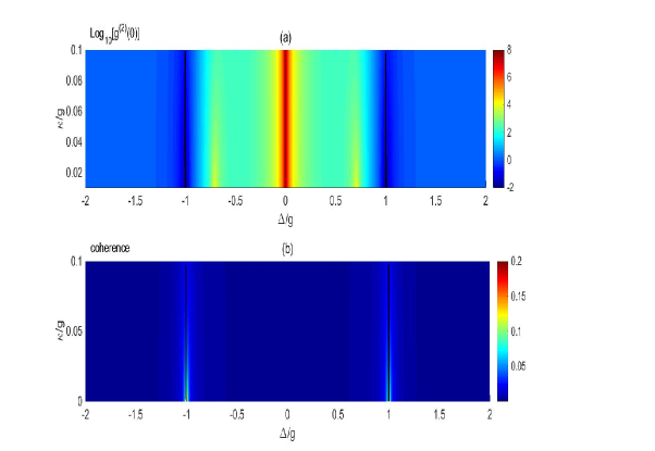
Figure 4: (color online). We plot logarithm of the equal-time second-order correlation function $\log_{10}\left[g^{(2)}(0)\right]$ and the atomic coherence as a function of the detuning $\Delta$ and cavity decay rate $\kappa$. (a) shows the second-order correlation function and (b) corresponds the atomic coherence. The optimal photon anti-bunching and the maximal atomic coherence are also illustrated by the black-solid line in (a) and (b) which corresponds to $\Delta^{2}=g^{2}$. Here, we set $\gamma/g=0.01$, $\eta/g=0.001$.

From Fig. 1 (b), it is obvious that the coherence has a pair of maximal values. Compared with Fig. 1 (a), one can easily find that the two points with the maximal coherence perfectly correspond to the optimal photon blockade, which means the maximal coherence of the atomic state can capture the photon blockade. In addition, one can also see that the maximal photon bunching point corresponds to the almost vanishing coherence instead of the maximal coherence. To better understand this correspondence relation, let us use the analytic expression given in Eq. (21) to analyze the results, from which one can see that the extremum occur at $\Delta=\pm g$ for small $\{\kappa,\gamma\}$. This is consistent with the analysis on the optimal photon anti-bunching condition. In order to give an intuitive understanding of this correspondence, one should note that once $\Delta=\pm g$, the driving field is tuned resonantly with the transition between $\left|0g\right\rangle$ and $\left|1,\pm\right\rangle$ which leads to the optimal photon blockade, meanwhile, the system will locate in the state $\bar{C}_{1g}\left|1,g\right\rangle+\bar{C}_{0e}\left|0,e\right\rangle$. Thus, the state of $\left|0,e\right\rangle$ is actually occupied with a relatively large probability which is proportional to the first order of the driving field $\eta$. It is obvious from Eq. (21) that $\left|\Psi\right\rangle$ owns the relatively large amount of coherence (see in Fig. 1 (b)). When the driving field is resonant to the two-photon process (the transition $\left|0,g\right\rangle$ to $\left|2,\pm\right\rangle)$, thus $\left|2,\pm\right\rangle$ occupies the relatively dominant proportion in $\left|\Psi\right\rangle$. However, the amplitude is proportional to the $\eta^{2}$. To the good approximation, we can omit it safely in Eq. (20). Thus, the coherence at these points do not get the extremum. In addition, it is interesting that the maximal photon bunching point at $\Delta=0$ (photon-induced tunnelling point) does not correspond to an extremum of coherence. At $\Delta=0,$ a quasi-dark state process occurs, the system being driven into a quasi-dark state $\left|d\right\rangle\thicksim g\left|0,g\right\rangle-\eta\left|0,e\right\rangle,$ which provides a channel to be converted to the state $\left|2,g\right\rangle$ as well as $\left|1,e\right\rangle$. Their proportions in $\left|\Psi\right\rangle$ get relatively larger. The net effect on coherence is that $\left|0,e\right\rangle$ reaches a suppression in the driven mode, so the coherence is negligibly small.

In addition, in order to find the general features of the correspondence relation, we plot the coherence and the logarithmic equal-time second-order correlation function with different $\Delta$ and $g$ in Fig. 3. From the Fig. 3, we can observe that optimal anti-bunching corresponds to the maximal coherence with small enough dissipations ($g,\Delta\gg\{\kappa,\gamma\}$) which are plotted by the white dashed lines in the Fig. 3 (a) and Fig. 3 (b). The condition for this correspondence relation can be demonstrated analytically from Eq. (15) and Eq. (21) as $\Delta^{2}=g^{2}.$ In addition, one can find that the dissipations of the cavity and atom have certain influence on both photon statistics and atomic coherence. We plot the effect of the cavity decay $\kappa$ on the correspondence relation in Fig. 4. We note that both the optimal photon statistics and the coherence extremals are reduced with $\kappa$ increasing. Meanwhile, the correspondence relation between coherence and $g^{2}(0)$ gets worse. Mathematically, this can be well understood from Eq. (15) and Eq. (21) from which one can see that all the relevant analysis are satisfied within the error region to the same order as $\kappa^{2}$. Physically, the inaccuracy obviously results from the increasing widths of the energy levels. So generally we always limit our study in the region with small enough dissipations for a good correspondence relation.

V Discussions and conclusion

To conclude, we have studied the photon statistics and the atomic coherence in a weakly driving CQED system and analyzed the physical mechanisms of photon statistics and coherence in details. We systematically study the system parameters’ dependence on the photon statistics and coherence. Our results gave a clear quantitative analysis and connections between atomic coherence and quantum statistics. By numerically solving the master equation in the steady state and calculating the equal time second-order correlation function and the atomic coherence, we obtained a perfect relation between the atomic coherence and the photon blockade, i.e., the maximal coherence always correspond to the optimal anti-bunching points. By the analytical way, we derive the analytical condition for the correspondence relation, which agrees well with the numerical simulation. In addition, the maximal photon bunching point corresponds to the almost vanishing coherence due to a quasi-dark-state process.

Finally, we would like to emphasize that this perfect match relation has been only found in the current special model after all. Whether this relation can exist in other model with much strong quantum blockade deserves us forthcoming research. If such a model could be found, one maybe could enhance the photon blockade by controlling the atomic coherence. In summary, we provided new insight into the rather unexplored area and could be potentially pivotal for future quantum applications.

VI Acknowledgements

Y Zhang thanks J. S. Jin for valuable discussion. This work was supported by the National Natural Science Foundation of China, under Grant No.11375036 and 11175033, the Xinghai Scholar Cultivation Plan and the Fundamental Research Funds for the Central Universities under Grants No. DUT15LK35 and No. DUT15TD47.

References

- (1) M. J. Werner and A. Imamoḡlu, “Photon-photon interactions in cavity electromagnetically induced transparency,” Phys. Rev. A 61, 011801(R) (1999).
- (2) H. Wang et al., “Tunable photon blockade in a hybrid system consisting of an optomechanical device coupled to a two-level system,” Phys. Rev. A 92,033806 (2015).
- (3) S. Ferretti, V. Savona and D. Gerace, “Optimal antibunching in passive photonic devices based on coupled nonlinear resonators,” New J. Phys. 15, 025012 (2013).
- (4) P. Rabl, “Photon Blockade Effect in Optomechanical Systems,” Phys. Rev. Lett. 107, 063601 (2011).
- (5) A. Nunnenkamp, K. Børkje, and S. M. Girvin, “Single-Photon Optomechanics,” Phys. Rev. Lett. 107, 063602 (2011).
- (6) P. Kómár et al., “Single-photon nonlinearities in two-mode optomechanics,” Phys. Rev. A 87, 013839 (2013).
- (7) J. Q. Liao and F. Nori, “Photon blockade in quadratically coupled optomechanical systems,” Phys. Rev. A 88, 023853 (2013).
- (8) Y. L. Liu, Z. P. Liu, and J. Zhang, “Coherent-feedback-induced controllable optical bistability and photon blockade,” J. Phys. B: At. Mol. Opt. Phys. 48, 105501 (2015).
- (9) A. J. Hoffman et al., “Dispersive Photon Blockade in a Superconducting Circuit,.” Phys. Rev. Lett. 107, 053602 (2011).
- (10) Y. X. Liu, X. W. Xu, A. Miranowicz, and F. Nori, “From blockade to transparency: Controllable photon transmission through a circuit-QED system,” Phys. Rev. A 89, 043818 (2014).
- (11) A. Reinhard et al., “Strongly correlated photons on a chip,” Nat. Photonics 6, 93 (2012).
- (12) K. M. Birnbaum et al, “Photon blockade in an optical cavity with one trapped atom,” Nature (London) 436, 87 (2005).
- (13) B. Dayan et al., “A Photon Turnstile Dynamically Regulated by One Atom,” Science 319, 1062 (2008) .
- (14) A. Verger, C. Ciuti, and I. Carusotto, “Polariton quantum blockade in a photonic dot,” Phys. Rev. B 73, 193306 (2006).
- (15) A. Faraon et al., “Climbing the Jaynes–Cummings ladder and observing its nonlinearity in a cavity QED system,”Nature . 454, 315 (2008).
- (16) K. Müller etal., “Coherent Generation of Nonclassical Light on Chip via Detuned Photon Blockade,” Phys. Rev. Lett. 114, 233601 (2015).
- (17) A. Kubanek etal., “Two-Photon Gateway in One-Atom Cavity Quantum Electrodynamics,” Phys. Rev. Lett. 101, 203602 (2008).
- (18) A. Faraon, A. Majumdar, and J. Vučković, “Generation of nonclassical states of light via photon blockade in optical nanocavities,” Phys. Rev. A 81, 033838 (2010).
- (19) A. Majumdar, E. D. Kim, Y. Y. Gong, M. Bajcsy, and J. Vučković, “Phonon mediated off-resonant quantum dot–cavity coupling under resonant excitation of the quantum dot,” Phys. Rev. B 84, 085309 (2011).
- (20) L. Tian and H. J. Carmichael, “Quantum trajectory simulations of the two-state behavior of an optical cavity containing one atom,” Phys. Rev. A 46, R6801 (1992).
- (21) D. E. Chang, V. Vuletić and M-D. Lukin, “Quantum nonlinear optics-photon by photon,” Nat. photonics 8, 685 (2014).
- (22) A. Majumdar, M. Bajcsy and J. Vučković, “Probing the ladder of dressed states and nonclassical light generation in quantum-dot-cavity QED,” Phys. Rev. A 85, 041801(R) (2012).
- (23) Y. Zhang, J. Zhang, S. X. Wu, and C. S. Yu, “The effect of center-of-mass motion on photon statistics,” Ann. Phy 361, 563 (2015).
- (24) A. Streltsovet et al., “Measuring Quantum Coherence with Entanglement,” Phys. Rev. Lett. 115, 020403 (2015).
- (25) M. Piani et al“Robustness of asymmetry and coherence of quantum states” arXiv:1601.03782
- (26) C. Napoli et al, “Robustness of coherence: An operational and observable measure of quantum coherence,” arXiv:1601.03781
- (27) D. Girolami, “Observable Measure of Quantum Coherence in Finite Dimensional Systems” Phys. Rev. Lett. 113, 170401 (2014).
- (28) A. Winter and D. Yang, “Operational Resource Theory of Coherence” Phys. Rev. Lett. 116, 120404 (2016).
- (29) A. Streltsov, “Genuine Quantum Coherence” arXiv:1511.08346
- (30) I. Marvian, R. W. Spekkens, and P. Zanardi, Quantum speed limits, coherence and asymmetry, arXiv:1510.06474
- (31) A. Albrecht, “Some Remarks on Quantum Coherence,” J. Mod. Opt. 41, 2467 (1994).
- (32) R. J. Glauber, “Coherent and Incoherent States of the Radiation Field,” Phys. Rev. 131, 2766 (1963).
- (33) M. O. Scully, “Enhancement of the Index of Refraction via Quantum Coherence,” Phys. Rev. Lett. 67, 1855 (1991).
- (34) T. Baumgratz, M. Cramer, and M.?B. Plenio, “Quantifying Coherence,” Phys. Rev. Lett. 113, 140401 (2014).
- (35) J. Åberg “Quantifying Superposition,” arXiv:quant-ph/0612146 (2006).
- (36) C. S. Yu, Y. Zhang, and H. Q. Zhao, “Quantum correlation via quantum coherence,” Quant. Inf. Proc. 13(6), 1437 (2014).
- (37) Y. Yao, X. Xiao, and C. P. Sun, “Quantum coherence in multipartite systems,” Phys. Rev. A 92, 022112 (2015).
- (38) Z. J. Xi, Y. M. Li, and H. Fan, “Quantum coherence and correlations in quantum system,” Sci. Rep 5, 10922 (2015).
- (39) M. Lostaglio, D. Jennings, and T. Rudolph, “Description of quantum coherence in thermodynamic processes requires constraints beyond free energy,” Nat. Commun. 6, 6383 (2015).
- (40) A. Monras, A. Checińska, and A. Ekert, “Witnessing quantum coherence in the presence of noise,” New J. Phys. 16, 063041 (2014).
- (41) L. Rybak et al., “Generating Molecular Rovibrational Coherence by Two-Photon Femtosecond Photoassociation of Thermally Hot Atoms,” Phys. Rev. Lett. 107, 273001 (2011).
- (42) G. Barontini, R. Labouvie, F. Stubenrauch, A. Vogler, V. Guarrera, and H. Ott, “Controlling the Dynamics of an Open Many-Body Quantum System with Localized Dissipation,” Phys. Rev. Lett. 110, 035302 (2013).
- (43) J. T. Barreiro et al., “An open-system quantum simulator with trapped ions,” Nature 470, 486 (2011).
- (44) J. Cai and M. B. Plenio, “Chemical Compass Model for Avian Magnetoreception as a Quantum Coherent Device,” Phys. Rev. Lett. 111, 230503 (2013).
- (45) A. Ishizaki and G. R. Fleming, “Theoretical examination of quantum coherence in a photosynthetic system at physiological temperature,” Proc. Natl. Acad. Sci. 106, 17255 (2009).
- (46) E. J. O’Reilly and A. Olaya-Castro, “Non-classicality of the molecular vibrations assisting exciton energy transfer at room temperature,” Nat. Commun. 5, 3012 (2014).
- (47) J. Åberg, “Catalytic Coherence,” Phys. Rev. Lett. 113, 150402 (2014).
- (48) L. A. Correa, J. P. Palao, D. Alonso, and G. Adesso, “Quantum-enhanced absorption refrigerators,” Sci. Rep. 4, 3949 (2014).
- (49) C. M. Li, N. Lambert, Y. N. Chen, G. Y. Chen, and F. Nori, “Witnessing Quantum Coherence: from solid-state to biological systems,” Sci. Rep. 2, 885 (2012).
- (50) P. Grünwald and W. Vogel, “Optimal Squeezing in Resonance Fluorescence via Atomic-State Purification,” Phys. Rev. Lett. 109, 013601 (2012).
- (51) H. Wang, D. Goorskey, and M. Xiao, “Enhanced Kerr Nonlinearity via Atomic Coherence in a Three-Level Atomic System,” Phys. Rev. Lett. 87, 073601 (2001).
- (52) M. Bajcsy, A. Majumdar, A Rundquist and J. Vučković,“Photon blockade with a four-level quantum emitter coupled to a photonic-crystal nanocavity,” New J. Phys. 15 025014 (2013).
- (53) S. E. Harris, “Electromagnetically induced transparency,” Phys. Today 50(7), 36 (1997).
- (54) M. Ebert, M. Kwon, T. G. Walker, and M. Saffman, “Coherence and Rydberg blockade of atomic ensemble qubits,” arXiv:1501.04083v4.
- (55) E. T. Jaynes and F. W, Cummings, “Comparison of quantum and semiclassical radiation theories with application to the beam maser,” Proc. IEEE 51, 89 (1963).
- (56) M. O. Scully and M. Suhail Zubairy, “Quantum optics” (Cambridge university press, 1997).
- (57) C. Lang et al., “Observation of Resonant Photon Blockade at Microwave Frequencies Using Correlation Function Measurements,” Phys. Rev. lett 106, 243601 (2011).
- (58) X. T. Zou and L. Mandel, “Photon-antibunching and sub-Poissonian photon statistics,” Phys. Rev. A 41, 475 (1990).
- (59) S. M. Tan, “A computational toolbox for quantum and atomic optics,” J. Opt. B: Quantum Semiclassical Opt. 1, 424 (1999).
- (60) X. W. Xu and Y. Li, “Strong photon antibunching of symmetric and antisymmetric modes in weakly nonlinear photonic molecules,” Phys. Rev. A 90, 033809 (2014).
- (61) X. W. Xu and Y. Li, “Tunable photon statistics in weakly nonlinear photonic molecules,” Phys. Rev. A 90, 043822 (2014).
- (62) H. J. Carmichael., “An Open Systems Approach to Quantum Optics,” Lecture Notes in Physics (Springer, Berlin, 1993).
- (63) I. Carusotto and C. Ciuti, “Quantum fluids of light,” Rev. Mod. Phys, 85, 299 (2013).
- (64) H. J. Carmichael, R. J. Brecha, and P. R. Rice, “Quantum interference and collapse of the wavefunction in cavity QED,” Opt. Commun. 82, 73 (1991).
- (65) H. J. Carmichael, “Photon Antibunching and Squeezing for a Single Atom in a Resonant Cavity,” Phys. Rev. Lett. 55, 2790 (1985).
- (66) D. F. Walls and G. J. Milburn, “ Quantum Optics” (Springer-Verlag, Berlin, Heidelberg, 1994).
- (67) C. S. Yu and H. S. Song, “Bipartite concurrence and localized coherence,” Phys. Rev. A 80, 022324 (2009).
- (68) O. T. Cunha, “The geometry of entanglement sudden death,” New J. Phys. 9, 237 (2007).
- (69) K. Ann and G. Jaeger, “Finite-time destruction of entanglement and non-locality by environmental influences,” Found. Phys. 39, 790 (2009).