A cosmologically motivated reference formulation of numerical relativity

Abstract

The application of numerical relativity to cosmological spacetimes is providing new insights into the behavior of Einstein’s equations, beyond common approximations. In order for simulations to be performed as accurately and efficiently as possible, we investigate a novel formulation of Einstein’s equations. This formulation evolves differences from a “reference” solution describing the dominant behavior of the spacetime, which mitigates error due to both truncation and approximate finite difference calculations. We find that the error in solutions obtained using the reference formulation can be smaller by an order of magnitude or more, with the level of improvement depending on how well the reference solution approximates the exact solution.

1 Introduction

Standard cosmological models contain a number of assumptions, often necessary in order to make these models tractable. One common assumption is that the gravitational physics can be simplified, as cosmological systems are often well-described by linearized gravity or Newtonian physics on an expanding homogeneous background. Yet, such assumptions have not been thoroughly tested and compared to predictions from the full theory of general relativity, leaving open the possibility that these simplifications result in an inaccurate or biased view of our Universe. Already, observations interpreted utilizing such assumptions have found moderate inconsistencies among inferred cosmological parameters [1, 2]. Exploring the validity of gravitational approximations with sufficient accuracy will require a careful, systematic analysis of cosmological models in a fully general relativistic setting.

A number of studies have speculated that quantities computed using approximate gravitational models in a cosmological context require percent-level corrections, with even larger corrections possible, depending on the quantity of interest [3, 4, 5]. Properly characterizing such phenomena will require modeling spacetimes with at least this accuracy and precision—a formidable task, even in the context of Newtonian gravity [6]. In order to explore ideas such as this, numerical relativity is being employed in a cosmological setting with increasing frequency [7, 8, 9, 10, 11, 12, 13].

As a unique method for improving the accuracy of cosmological simulations in full general relativity, we explore a cosmologically-motivated “reference formulation” in which the fully relativistic differences from an approximate, semi-analytic background solution are computed. It should be noted that this is simply a reformulation of Einstein’s equations, not an application of perturbation theory, nor an approximation of Einstein’s equations. The potential benefits of this method are twofold: first, resolving gravitational physics that could not otherwise be resolved due to roundoff error, and second, minimizing error contributions due to finite differencing.

We study the accuracy of this method primarily in a cosmological setting, evolving a universe filled with a pressureless “dust” perfect fluid. We find that the method fares well when the reference solution is a good description of the spacetime, reducing solution error by an order-of-magnitude or more, with this advantage decreasing as the spacetime evolves further away from the reference solution.

In Sec. 2 we develop the reference formulation with cosmological applications in mind, first presenting details of the standard BSSNOK system in Sec. 2.1, then extending the formulation to account for the reference solution in Sec. 2.2. In Sec. 3 we describe initial conditions for a cosmologically-motivated test of the reference formulation, and explore the behavior of simulation error in the reference formulation compared to the standard BSSNOK formulation in Sec. 4.

2 Constructing a reference formulation

2.1 The BSSNOK Formulation

Over the past decade, a variety of formulations of general relativity have been developed for numerical integration, and have demonstrated their ability to accurately model strongly gravitating systems with numerically stability. Perhaps the most commonly used is the BSSNOK formulation, a conformal 3+1 decomposition of the Einstein field equations [14, 15, 16]. In this decomposition, the line element is given by

$$ds^{2}=-\alpha^{2}dt^{2}+\gamma_{ij}\left(dx^{i}+\beta^{i}dt\right)\left(dx^{j}+\beta^{j}dt\right)\,,$$ (1)

where $\alpha$ and $\beta^{i}$ are gauge variables, respectively known as the lapse and shift. The spatial metric, $\gamma_{ij}$, is decomposed into a conformal metric, $\bar{\gamma}_{ij}$, and conformal factor, $\phi$, as $\gamma_{ij}=e^{4\phi}\bar{\gamma}_{ij}$, where the conformal metric has unit determinant and $\det\gamma_{ij}=e^{12\phi}$.

When written in terms of these variables, the Einstein field equations are equivalent to the standard BSSNOK equations,

$$\partial_{t}\phi= -\frac{1}{6}\alpha K+\beta^{i}\partial_{i}\phi+\frac{1}{6}\partial_{i}\beta^{i}$$ (2)

$$\partial_{t}\bar{\gamma}_{ij}= -2\alpha\bar{A}_{ij}+\beta^{k}\partial_{k}\bar{\gamma}_{ij}+\bar{\gamma}_{ik}\partial_{j}\beta^{k}+\bar{\gamma}_{kj}\partial_{i}\beta^{k}-\frac{2}{3}\bar{\gamma}_{ij}\partial_{k}\beta^{k}$$ (3)

$$\partial_{t}K= -\gamma^{ij}D_{j}D_{i}\alpha+\alpha(\bar{A}_{ij}\bar{A}^{ij}+\frac{1}{3}K^{2})+4\pi\alpha(\rho+S)+\beta^{i}\partial_{i}K$$ (4)

$$\partial_{t}\bar{A}_{ij}= e^{-4\phi}(-(D_{i}D_{j}\alpha)+\alpha(R_{ij}-8\pi S_{ij}))^{TF}+\alpha(K\bar{A}_{ij}-2\bar{A}_{il}\bar{A}_{j}^{l})$$ (5)

$$+\beta^{k}\partial_{k}\bar{A}_{ij}+\bar{A}_{ik}\partial_{j}\beta^{k}+\bar{A}_{kj}\partial_{i}\beta^{k}-\frac{2}{3}\bar{A}_{ij}\partial_{k}\beta^{k}\,.$$

Here, the stress-energy tensor has been projected onto the spatial hypersurfaces of the decomposition, resulting in source terms for the BSSNOK metric fields, $\rho$, $S_{ij}$, and $S=\gamma^{ij}S_{ij}$. The variable $K$ is the trace of the extrinsic curvature $K_{ij}$, and $\bar{A}_{ij}$ is the conformally related trace-free part of the extrinsic curvature,

$$e^{4\phi}\bar{A}_{ij}=K_{ij}-\frac{1}{3}\gamma_{ij}K\,.$$ (6)

In general, quantities with bars are raised, lowered, and computed using the conformal metric $\bar{\gamma}_{ij}$, and unbarred quantities with the full 3-metric, $\gamma_{ij}$.

In the BSSNOK formulation, additional auxiliary variables are introduced to improve stability of the system. A contraction of a Christoffel symbol of the conformal metric is evolved,

$$\partial_{t}\bar{\Gamma}^{i}= -2\bar{A}^{ij}\partial_{j}\alpha+2\alpha\left(\bar{\Gamma}_{jk}^{i}\bar{A}^{jk}-\frac{2}{3}\bar{\gamma}^{ij}\partial_{j}K-8\pi\bar{\gamma}^{ij}S_{j}+6\bar{A}^{ij}\partial_{j}\phi\right)$$ (7)

$$+\beta^{j}\partial_{j}\bar{\Gamma}^{i}-\bar{\Gamma}^{j}\partial_{j}\beta^{i}+\frac{2}{3}\bar{\Gamma}^{i}\partial_{j}\beta^{j}+\frac{1}{3}\bar{\gamma}^{li}\partial_{l}\partial_{j}\beta^{j}+\bar{\gamma}^{lj}\partial_{l}\partial_{j}\beta^{i}\,,$$

where $\bar{\Gamma}^{i}=\bar{\gamma}^{jk}\bar{\Gamma}_{jk}^{i}$. A more comprehensive introduction to this formulation of numerical relativity, and the motivation behind this scheme, can be found in textbooks such as [17] and [18].

2.2 A Cosmologically Motivated Reference Formulation

For many spacetimes, there are known solutions of the Einstein (and thus BSSNOK) equations that describe the spacetime, both approximate and exact, with deviations from such solutions expected to be small. The focus of this paper is to examine the behavior of solution error of simulations in a cosmological setting obtained by evolving deviations from dominant reference functions, rather than directly using the BSSNOK equations themselves. These reference functions need not be actual solutions to the Einstein field equations, and need not be known analytically. The goal will be to use such reference functions to reduce the susceptibility of calculations to truncation error or to errors from taking finite differences.

Similar ideas have been explored before [19], particularly in the context of coordinate systems with singularities such as spherical polar coordinates [20]. However, to our knowledge, more general reference functions have not been used.

In a matter-dominated cosmology in geodesic slicing, the dominant solution can be described purely by several variables of interest. We will be evolving differences between these variables and the full BSSNOK variables. We denote difference variables by $\Delta$’s, and define them in terms of reference functions (hatted) and standard BSSNOK metric variables,

$$\Delta\bar{\gamma}_{ij} \equiv\bar{\gamma}_{ij}-\delta_{ij}$$ (8)

$$\Delta\bar{\gamma}^{ij} \equiv\bar{\gamma}^{ij}-\delta^{ij}$$ (9)

$$\Delta\phi \equiv\phi-\hat{\phi}$$ (10)

$$\Delta K \equiv K-\hat{K}$$ (11)

$$\Delta\Gamma^{i} \equiv\Gamma^{i}-\hat{\Gamma}^{i}$$ (12)

$$\Delta\rho \equiv\rho-\hat{\rho}\,.$$ (13)

with the remaining metric variable $\bar{A}_{ij}$ being zero. Additional details regarding computing metric components can be found in A. Once expressions for the evolution of the reference variables have been specified, they can be subtracted from the BSSNOK equations in order to form evolution equations for the difference variables. Because the BSSNOK equations involve only differentiation and multiplication, the leading-order contributions to the BSSNOK equations from the reference solution can be canceled.

Performing this procedure for the differenced conformal metric $\Delta\bar{\gamma}_{ij}$ is straightforward, as the reference metric is taken to be $\delta_{ij}$, which does not change. The right-hand side of the evolution equations for the difference metric is therefore identical to the BSSNOK equations,

$$\partial_{t}\Delta\bar{\gamma}_{ij}\equiv\partial_{t}\bar{\gamma}_{ij}\,.$$ (14)

The remaining variables are chosen to be an approximate solution to the Einstein field equations. For cosmological systems, an approximate solution for a pressureless perfect fluid with zero velocity in geodesic slicing may be found by neglecting $\mathcal{O}(\bar{A}_{ij}^{2})$ terms in the evolution equations for $K$ and $\phi$, as in [9]. Evolution equations for the conformal factor and the trace of the extrinsic curvature therefore obey a set of coupled ODEs at each point,

$$\partial_{t}\hat{\phi} = -\frac{1}{6}\alpha\hat{K}\,,$$ (15)

$$\partial_{t}\hat{K} = \frac{1}{3}\alpha\hat{K}^{2}+4\pi\alpha\hat{\rho}\,.$$ (16)

These equations describe each location in the universe as obeying a locally-FLRW equation. In principle, because fluctuations around this solution are small on the scales of interest (as shown in [9]), the precision with which algebraic operations can be performed is increased.

Deviations of the extrinsic curvature from the reference solution will subsequently be sourced only by the neglected $\bar{A}_{ij}\bar{A}^{ij}$ term. This variable, in turn, is both self-sourced, and sourced by the (trace-free) Ricci tensor. The dominant contribution to the Ricci tensor comes from derivatives of the conformal factor; thus, accurately determining these derivatives is important.

The dominant source of error comes from discretization, or from computing derivatives using finite-difference stencils. To minimize the contribution of this error, we also evolve the gradients of the reference variables locally,

$$\partial_{t}\hat{\phi}_{,i} = -\frac{1}{6}\alpha\hat{K}_{,i}$$ (17)

$$\partial_{t}\hat{K}_{,i} = \frac{2}{3}\alpha\hat{K}\hat{K}_{,i}+4\pi\alpha\hat{\rho}_{,i}$$ (18)

$$\partial_{t}\hat{\phi}_{,ij} = -\frac{1}{6}\alpha\hat{K}_{,ij}$$ (19)

$$\partial_{t}\hat{K}_{,ij} = \frac{2}{3}\alpha\hat{K}_{,i}\hat{K}_{,j}+\frac{2}{3}\alpha\hat{K}\hat{K}_{,ij}+4\pi\alpha\hat{\rho}_{,ij}\,,$$ (20)

from which gradients of BSSNOK fields can be constructed using, eg., $\partial_{i}\phi=\hat{\phi}_{,i}+\partial_{i}\Delta\phi$. Additional reference variables can be defined for each of the remaining metric variables. The most straightforward of these to write is an equation for the conformal Christoffel and its derivative,

$$\partial_{t}\hat{\bar{\Gamma}}^{i} = -\frac{4}{3}\alpha\delta^{ij}\hat{K}_{,j}\,,$$ (21)

$$\partial_{t}\hat{\bar{\Gamma}}_{,k}^{i} = -\frac{4}{3}\alpha\delta^{ij}\hat{K}_{,jk}\,.$$ (22)

In principle, an equation for the conformal 3-metric (beyond the flat-space contribution) and its time derivative $\bar{A}_{ij}$ could be written. However, the evolution equation for $\bar{A}_{ij}$ is sourced by the Ricci tensor, which requires evolving derivatives of the conformal factor and conformal metric, which in turn would require evolving derivatives of ever-increasing order. This procedure could nevertheless be performed and truncated at some order (even at lowest order, i.e. $\bar{A}_{ij}$ could be sourced purely by the Ricci tensor assuming $\bar{\gamma}_{ij}=\delta_{ij}$); however, we leave such an idea for future work.

Finally, the system is closed by evolving a pressureless perfect-fluid stress-energy source mimicking a dark matter component. Such a fluid at rest in geodesic slicing obeys a simple conservation law,

$$\partial_{t}D=\partial_{t}\hat{D}=0\,,$$ (23)

where the reference and standard density variables are given by

$$\hat{D} \equiv \alpha e^{6\hat{\phi}}\hat{\rho}$$ (24)

$$D \equiv \alpha e^{6\phi}\rho\,.$$ (25)

The gradients of the source, $\hat{\rho}_{,i}$ and $\hat{\rho}_{,ij}$ can be derived from these expressions,

$$\hat{\rho}_{,i} = -6\hat{\rho}\hat{\phi}_{,i}+\frac{1}{\alpha}e^{-6\hat{\phi}}\hat{D}_{,i}$$ (26)

$$\hat{\rho}_{,ij} = -3\left(\hat{\rho}_{,j}\hat{\phi}_{,i}+\hat{\rho}_{,i}\hat{\phi}_{,j}+2\hat{\rho}\hat{\phi}_{,ij}\right)+\frac{-3}{\alpha}e^{-6\hat{\phi}}\left(\hat{D}_{,i}\hat{\phi}_{,j}+\hat{D}_{,j}\hat{\phi}_{,i}-\frac{1}{3}\hat{D}_{,ij}\right)\,,$$ (27)

where the right-hand side of Eq. 27 has additionally been symmetrized in the $i$ and $j$ indices.

Subtracting the equations of motion from the BSSNOK equations yields a set of equations for the corresponding difference variables,

$$\begin{array}[]{lll}\partial_{t}\Delta\phi&=&\partial_{t}\phi-\partial_{t}\hat{\phi}\\ &=&-\frac{1}{6}\alpha\Delta K+\beta^{i}\partial_{i}\phi+\frac{1}{6}\partial_{i}\beta^{i}\end{array}$$ (28)

$$\begin{array}[]{lll}\partial_{t}\Delta K&=&\partial_{t}K-\partial_{t}\hat{K}\\ &=&-\gamma^{ij}D_{j}D_{i}\alpha+\alpha\bar{A}_{ij}\bar{A}^{ij}+\frac{1}{3}\alpha\left(\Delta K+2\hat{K}\right)\Delta K\\ &&+4\pi\alpha\Delta\rho+4\pi\alpha S+\beta^{i}\partial_{i}K\end{array}$$ (29)

$$\begin{array}[]{lll}\partial_{t}\Delta\bar{\gamma}_{ij}&=&\partial_{t}\bar{\gamma}_{ij}\\ &=&-2\alpha\bar{A}_{ij}+\beta^{k}\partial_{k}\bar{\gamma}_{ij}+\bar{\gamma}_{ik}\partial_{j}\beta^{k}+\bar{\gamma}_{kj}\partial_{i}\beta^{k}-\frac{2}{3}\bar{\gamma}_{ij}\partial_{k}\beta^{k}\end{array}$$ (30)

$$\begin{array}[]{lll}\partial_{t}\Delta\hat{\bar{\Gamma}}^{i}&=&\partial_{t}\bar{\Gamma}^{i}-\partial_{t}\hat{\bar{\Gamma}}^{i}\\ &=&-2\bar{A}^{ij}\partial_{j}\alpha+2\alpha\bar{\Gamma}_{jk}^{i}\bar{A}^{jk}\\ &&-\frac{4\alpha}{3}\left(\bar{\gamma}^{ij}\partial_{j}\Delta K+\Delta\bar{\gamma}^{ij}\partial_{j}\hat{K}-8\pi\bar{\gamma}^{ij}S_{j}+6\bar{A}^{ij}\partial_{j}\phi\right)\\ &&+\beta^{j}\partial_{j}\bar{\Gamma}^{i}-\bar{\Gamma}^{j}\partial_{j}\beta^{i}+\frac{2}{3}\bar{\Gamma}^{i}\partial_{j}\beta^{j}+\frac{1}{3}\bar{\gamma}^{li}\partial_{l}\partial_{j}\beta^{j}+\bar{\gamma}^{lj}\partial_{l}\partial_{j}\beta^{i}\,.\end{array}$$ (31)

An important point here is that the equations for the difference variables contain no zeroth-order components, and the dominant contribution to gradients can be computed using reference values so long as the reference solution remains a good approximate description of the spacetime.

3 Setting initial conditions

In order to specify initial conditions, we require field configurations that satisfy both the Hamiltonian and momentum constraint equations,

$$0 =\mathcal{H} =R+K^{2}-K_{ij}K^{ij}-16\pi\rho$$ (32)

$$0 =\mathcal{M}^{i} =D_{j}(K^{ij}-\gamma^{ij}K)-8\pi S^{i}\,.$$ (33)

As we are interested in comparing the accuracy of evolution between methods, setting analytic initial conditions is desirable. We simplify the constraint equations by setting the trace-free part of the extrinsic curvature to zero, $\bar{A}_{ij}=0$, and choosing the metric to be conformally flat, $\bar{\gamma}_{ij}=\delta_{ij}$. We can then obtain a solution by specifying the metric variables $\phi(\vec{x})$ and $K={\rm const}$, letting $\rho=\rho_{K}+\rho_{\phi}$, and algebraically solving the Hamiltonian constraint equation for the density variables,

$$K^{2} = 24\pi\rho_{K}\,,$$ (34)

$$\nabla^{2}e^{\phi} = -2\pi e^{5\phi}\rho_{\phi}\,.$$ (35)

This decomposition provides us with the physical metric variables, but a further choice is required in order to determine initial conditions for the reference variables. A straightforward choice is to simply use an FLRW solution close to the above initial conditions. However, this will only reduce roundoff error, not finite differencing error. Thus we instead choose to place all fluctuations in the reference variables themselves,

$$\hat{\rho} = \rho$$ (36)

$$\hat{\phi} = \phi$$ (37)

$$\hat{K} = K$$ (38)

so that the difference variables are all initially zero.

Choosing the conformal density $D$ to be entirely in the reference solution, $D=\hat{D}$, also allows the density reference variable to be computed using this variable,

$$\Delta\rho=\hat{\rho}\,\left[e^{-6\Delta\phi}-1\right]\,,$$ (39)

where the expression in brackets can be evaluated using a function designed to be accurate for small arguments.

For the purposes of this work, we examine two solutions in a periodic spacetime: one containing a single wavelength in the $x$-direction, and one containing a 3-dimensional solution $\phi$-mode in each direction. For these solutions, the conformal factor on the initial slice is respectively chosen to be

$$\phi_{1D} = A\sin(2\pi x+\varphi_{x})$$ (40)

$$\phi_{3D} = A\sin(2\pi x+\varphi_{x})\sin(2\pi y+\varphi_{y})\sin(2\pi z+\varphi_{z})$$ (41)

for some amplitude $A$ that ensures the density is positive everywhere, and arbitrary phases $\varphi_{i}$. Fluctuations in the fluid density are then reconstructed using Eq. 35.

The metric and matter variables can now be fully determined. We choose metric variables in terms of the Hubble scale on the initial slice, $H_{I}^{-1}$, so that

$$\rho_{K}=\frac{3}{8\pi}H_{I}^{2}$$ (42)

and the trace of the extrinsic curvature is $K=-3H_{I}$. The physical simulation volume is chosen to be $L^{3}=(H_{I}^{-1}/2)^{3}$.

4 Results

The main results we present are from simulations in which the sinusoidal metric fluctuations presented in Sec. 3 are resolved by as few points as is necessary to obtain results. For these simulations, we demonstrate the ability of the reference formulation to reduce error in the simulation, and study the behavior as both resolution and finite-difference-method order are increased, and as the solution evolves away from the analytic solution.

Although these tests demonstrate the ability of reference formulations to reduce error, they do not demonstrate the ability of the method to resolve fluctuations on a dominant background spacetime beyond the level of standard formulations. Therefore, in B we present additional runs of a linearized gravitational wave propagating through a flat spacetime.

As finite differences must still be computed in the reference formulation, the method order and convergence rate should remain similar to that of a standard, non-reference formulation. However, the amplitude of fluctuations around the analytic solution are expected to be smaller in the reference formulation, and to an extent smoother, leading to smaller errors when finite differences must be computed.

For cosmological runs, there are a number of ways to quantify the error of the system. In Figure 1, we present the amplitude of constraint violation in standard and reference formulations, for a simulation using Eq. 40 to set initial conditions. These are plotted against the volume-weighted average conformal factor of the spacetime, which increases monotonically with time, and corresponds to roughly half the number of e-folds of cosmological expansion the simulation has undergone.

The amplitude of fluctuations of the conformal factor is $A=2\times 10^{-4}$, resulting in a conformal standard deviation of the density $\sigma_{\rho}/\bar{\rho}\sim 0.05$ on the initial slice, and a minimum and maximum overdensity $\delta_{\rho}/\bar{\rho}\sim 0.1$. We use a very small timestep, $\Delta t=10^{-4}\Delta x$, to ensure time-integration convergence of solutions so that a meaningful comparison of error arising from discretization effects can be made. The simulations are then run until the worst-case surpasses $\sim 10\%$ Hamiltonian constraint violation amplitude relative to the energy scale of the problem, or the maximum $\mathcal{H}/[\mathcal{H}]>0.01$ for

$$[\mathcal{H}]=\frac{e^{5\phi}}{8}\sqrt{\bar{R}^{2}+\left(\frac{2}{3}K^{2}\right)^{2}+(A_{ij}A^{ij})^{2}+(16\pi\rho)^{2}}\,.$$ (43)

Runs are performed using a minimal resolution, $N=6$ in the direction containing fluctuations, with as few points as necessary to compute finite differences in other directions. Finite differences are also computed with minimal accuracy, with error of order $\mathcal{O}(\Delta x^{2})$, and compared to an $\mathcal{O}(\Delta x^{4})$ method.

From Fig. 1, we observe that the amplitude of measured constraint violation is smaller when taking advantage of the reference solution. The benefit of the reference formulation is most pronounced at early simulation times when the solution is closest to the reference solution. As the simulation evolves, deviating further from the reference solution, the relative benefit of the formulation decreases.

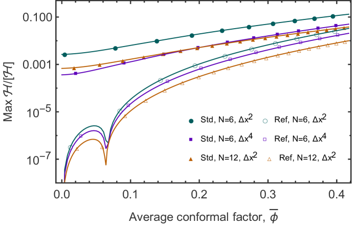
Figure 1: Hamiltonian constraint violation vs the volume-averaged conformal factor (roughly, half the number of cosmological e-folds of expansion undergone) for various 1-dimensional runs. Run parameters are indicated by the legend, including resolution ($N$ being the number of points in the $x$-direction, with a minimal number of points in other directions due to the symmetry of the simulation), finite-difference stencil order (accurate to $\mathcal{O}(\Delta x^{p})$), and method type being either the reference formulation (‘Ref’, open shapes) or the standard BSSNOK formulation (‘Std’, filled shapes). In general, the amount of constraint violation is found to be smaller using the reference formulation.

Beyond the improvement seen when increasing resolution or method order, or when using the reference formulation, there are additional noteworthy features. First, despite the use of analytic initial conditions, runs using the standard BSSNOK formulation mis-infer the amount of constraint violation present due to finite differencing error, resulting in a non-zero measurement of constraint violation on the initial surface. The reference formulation is, at least initially, able to compute the amount of constraint violation to within machine precision. Although the amount of error in the simulations does grow, the error demonstrates appropriate convergence for both formulations.

As computing the amplitude of constraint violation itself requires evaluating finite differences, it suffers from precisely the type of error we are trying to mitigate. Therefore, looking solely at the constraint violation does not provide the best measure of error. Because we are running at a low resolution, we can simply compare to higher resolution runs to obtain a more meaningful comparison. A solution obtained with $N=120$ using an 8th-order finite-difference method is taken to be the true solution, and deviations from this solution are plotted in Figure 2.

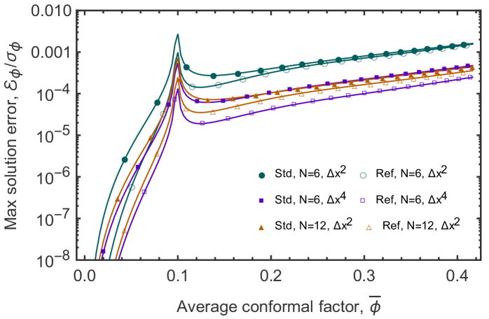
Figure 2: Solution error relative to an $N=120$ simulation as a function of the average conformal factor, $\bar{\phi}$ (a stand-in for time). Simulations performed using the reference formulation are seen to be more accurate, especially at early times when the reference solution is a good approximation.

As with the constraint violation measure, a relative benefit can be seen when using the reference formulation. For these runs, the maximum solution error of the local conformal factor $\varepsilon_{\phi}\equiv|\phi-\phi_{\rm true}|$ is plotted relative to the RMS amplitude of the fluctuations, $\sigma_{\phi}$, so as to emphasize the accuracy with which these fluctuations have been computed rather than the accuracy with which the dominant background cosmology has been computed. Again, the relative benefit is seen to be largest at early times, when the solution is well-described by the approximate reference solution. In this case, the formulation offers an order-of-magnitude benefit, and can be seen to perform better than doubling either the resolution or method order. At late times, however, the relative benefit disappears.

Several final points are of note. First, the reduction in relative error is seen to be somewhat greater for higher finite difference orders, which we speculate is due to the increased smoothness of the reference solution. Second, a spike in the relative error appears around $\bar{\phi}=0.1$. This is due to a brief drop in the value of $\sigma_{\phi}$ as it is driven from initial anti-correlation with density fluctuations towards becoming correlated (a behavior which can be viewed as a peculiarity of geodesic slicing). Finally, although not plotted here, the relative benefit at late times is found to be larger for smaller amplitude fluctuations, i.e. when the reference solution is a better approximation.

We additionally show the results of a 3-dimensional simulation with $N^{3}$ points, with initial conditions described by Eq. 41. These simulations are again run until thee worst case has surpassed roughly 10%-level constraint violation. Results from these runs are plotted in Figures 3 and 4. For these runs, we find similar results when looking at the level of computed constraint violation: the reference formulation yields a substantially smaller inferred level of constraint violation. However, again, the solution error should provide a better measure of simulation accuracy. For a low-order finite difference method, the advantage of the reference formulation disappears as the evolution progresses far enough away from the analytic solution. This remains true at higher resolutions, but is no longer true for a higher order finite difference method, suggesting that this is due to the numerical solution obtained using the reference formulation becoming insufficiently smooth at the level of the order of the finite difference error. However, for higher-order methods where finite differences are computed more accurately, the reference formulation maintains a significant advantage for the duration of the simulation. For both methods and for all choices of numerical and physical parameters, proper numerical convergence is found.

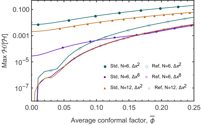
Figure 3: Hamiltonian constraint violation as a function of the volume-averaged conformal factor for various 3-dimensional runs. Run parameters are indicated by the legend, as in previous figures. As with the 1-dimensional case, the computed amount of constraint violation is smaller when using the reference formulation.

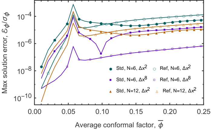
Figure 4: Solution error as a function of the average conformal factor, $\bar{\phi}$. Simulations performed using the reference formulation are found to be more accurate at early times, although less accurate at late times when using a low-order finite difference method.

5 Discussion

We have presented results from a cosmological reference formulation in which the dominant behavior of the spacetime dynamics was well-described by an approximate reference solution. The formulation was seen to provide more accurate results when the reference solution was a good description of the spacetime, and to nevertheless converge even when the reference solution was no longer a good approximation. The reference formulation was also found to be increasingly accurate relative to the non-reference formulation as method order increased.

Several improvements to the cosmological reference formulation presented here can be made that would ostensibly decrease simulation error. The evolution could use a slicing condition with improved stability properties, such as Harmonic slicing. In addition to the reference variables shown above, such a gauge would also require introducing a reference lapse, and spatial derivatives of the lapse. A second improvement would be to evolve the conformal metric and extrinsic curvature components sourced by all terms that do not require computing finite differences.

As we work to simulate cosmological systems in a fully relativistic setting with increasing realism, obtaining accurate results as efficiently as possible is an important goal. This formulation has demonstrated the ability to obtain reliable results and considerably decrease the numerical error without making any additional approximations.

References

Appendix A Accurate calculation of algebraic quantities

From the definitions in Sec. 2.2, care should be taken when raising and lowering indices of difference variables so that they are not directly raised and lowered using the 3-metric $\bar{\gamma}_{ij}$. Given a known difference metric $\Delta\bar{\gamma}_{ij}$, the difference of the inverse can be computed in an algebraic manner by explicitly writing out matrix components inverting, and subtracting. Noting that both $\det\bar{\gamma}_{ij}=\det\hat{\bar{\gamma}}_{ij}=1$, the end result of this operation results in matrix components

$$\Delta\bar{\gamma}^{11} = \hat{\bar{\gamma}}_{33}\Delta\bar{\gamma}_{22}-\Delta\bar{\gamma}_{23}(2\hat{\bar{\gamma}}_{23}+\Delta\bar{\gamma}_{23})+(\hat{\bar{\gamma}}_{22}+\Delta\bar{\gamma}_{22})\Delta\bar{\gamma}_{33}$$

$$\Delta\bar{\gamma}^{12} = -\hat{\bar{\gamma}}_{33}\Delta\bar{\gamma}_{12}+\hat{\bar{\gamma}}_{23}\Delta\bar{\gamma}_{13}+(\hat{\bar{\gamma}}_{13}+\Delta\bar{\gamma}_{13})\Delta\bar{\gamma}_{23}-(\hat{\bar{\gamma}}_{12}+\Delta\bar{\gamma}_{12})\Delta\bar{\gamma}_{33}$$

$$\Delta\bar{\gamma}^{13} = \hat{\bar{\gamma}}_{23}\Delta\bar{\gamma}_{12}-\hat{\bar{\gamma}}_{22}\Delta\bar{\gamma}_{13}-(\hat{\bar{\gamma}}_{13}+\Delta\bar{\gamma}_{13})\Delta\bar{\gamma}_{22}+(\hat{\bar{\gamma}}_{12}+\Delta\bar{\gamma}_{12})\Delta\bar{\gamma}_{23}$$

$$\Delta\bar{\gamma}^{22} = \hat{\bar{\gamma}}_{33}\Delta\bar{\gamma}_{11}-\Delta\bar{\gamma}_{13}(2\hat{\bar{\gamma}}_{13}+\Delta\bar{\gamma}_{13})+(\hat{\bar{\gamma}}_{11}+\Delta\bar{\gamma}_{11})\Delta\bar{\gamma}_{33}$$

$$\Delta\bar{\gamma}^{23} = -\hat{\bar{\gamma}}_{23}\Delta\bar{\gamma}_{11}+\hat{\bar{\gamma}}_{13}\Delta\bar{\gamma}_{12}+(\hat{\bar{\gamma}}_{12}+\Delta\bar{\gamma}_{12})\Delta\bar{\gamma}_{13}-(\hat{\bar{\gamma}}_{11}+\Delta\bar{\gamma}_{11})\Delta\bar{\gamma}_{23}$$

$$\Delta\bar{\gamma}^{33} = \hat{\bar{\gamma}}_{22}\Delta\bar{\gamma}_{11}-\Delta\bar{\gamma}_{12}(2\hat{\bar{\gamma}}_{12}+\Delta\bar{\gamma}_{12})+(\hat{\bar{\gamma}}_{11}+\Delta\bar{\gamma}_{11})\Delta\bar{\gamma}_{22}\,.$$ (44)

All terms in these equations are, notably, multiples of difference metric components; thus for small differences from the reference metric, components of the inverse metric are also small. Conformal Christoffel symbols are also computed using the difference metric,

$$\bar{\Gamma}_{ijk}=\frac{1}{2}\left(\partial_{j}\Delta\bar{\gamma}_{ik}+\partial_{k}\Delta\bar{\gamma}_{ij}-\partial_{i}\Delta\bar{\gamma}_{jk}\right)\,.$$ (45)

Appendix B Linearized Gravitational Wave Test

In this section we present results from a small-amplitude, linearized gravitational wave test around flat space. This is precisely the Apples with Apples linearized wave test [21], however the amplitude is substantially reduced in order to demonstrate the ability of the formulation to resolve small fluctuations around a dominant background—in this case, simply the flat, Minkowski metric.

The noteworthy feature here is that differences from $\delta_{ij}$ are evolved directly. For diagonal metric components in particular, this means that the dominant ‘1’ does not factor into roundoff error. While this particular test shows that features of such small amplitudes can be resolved, it does not demonstrate the ability of the method to model nonlinear physics more accurately, as is the intent behind the main results in Sec. 4.

The linearized wave Apples with Apples (AwA) test examines a linearized gravitational wave solution whose metric is of the form

$$ds^{2}=-dt^{2}+dx^{2}+(1+H)dy^{2}+(1-H)dz^{2}\,,$$ (46)

with

$$H=A\sin(2\pi(x-t))\,,$$ (47)

for a unit length box. The simulation is run for 1000 box-crossing times and checked against the analytic solution. The value of $A$ here is usually taken to be $A=10^{-8}$, so that terms of order $A^{2}$ will be at the level of roundoff error, or a part in $10^{16}$ when compared to the dominant ‘1’ of the flat metric. Here we will present results from a run with $A=10^{-16}$ so that second-order terms are still at the level of roundoff. However, they will now be at the level of roundoff relative to the amplitude of the gravitational wave itself.

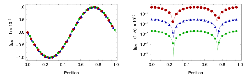
Figure 5: Results from the AwA linear wave test with a very small wave amplitude. Shown is the numerical solution for $g_{zz}$, and the difference of this solution from the analytic, linear solution ($1-H$) after 1000 box-crossing times. Good agreement with the analytic answer demonstrates the ability of the formulation to resolve very small fluctuations around a background spacetime. The test is run for 3 resolutions: 50 points (red, circles), 100 points (blue, triangles), and 200 points (green, squares).

As per test specifications, the simulation was run for 1000 box-crossing times with a timestep $\Delta t=\Delta x/4$. Results from this test are shown in Fig. 5. The observed convergence rate is in agreement with a method accurate to 4th-order in $\Delta x$, consistent with the dominant simulation error arising from the RK4 integration scheme used. Finite difference stencils were computed using an 8th-order scheme.

References

- [1] L. Verde, P. Protopapas, and R. Jimenez, “Planck and the local Universe: Quantifying the tension,” Phys. Dark Univ. 2 (2013) 166–175, arXiv:1306.6766 [astro-ph.CO].
- [2] J. L. Bernal, L. Verde, and A. G. Riess, “The trouble with ,” JCAP 1610 (2016) no. 10, 019, arXiv:1607.05617 [astro-ph.CO].
- [3] C. Clarkson, G. Ellis, J. Larena, and O. Umeh, “Does the growth of structure affect our dynamical models of the universe? The averaging, backreaction and fitting problems in cosmology,” Rept. Prog. Phys. 74 (2011) 112901, arXiv:1109.2314 [astro-ph.CO].
- [4] G. Ellis, R. Maartens, and M. MacCallum, Relativistic Cosmology. Cambridge University Press, 2012. https://books.google.com/books?id=IgkhAwAAQBAJ.
- [5] P. Fleury, C. Clarkson, and R. Maartens, “How does the cosmic large-scale structure bias the Hubble diagram?,” JCAP 1703 (2017) no. 03, 062, arXiv:1612.03726 [astro-ph.CO].
- [6] A. Schneider, R. Teyssier, D. Potter, J. Stadel, J. Onions, D. S. Reed, R. E. Smith, V. Springel, F. R. Pearce, and R. Scoccimarro, “Matter power spectrum and the challenge of percent accuracy,” JCAP 1604 (2016) no. 04, 047, arXiv:1503.05920 [astro-ph.CO].
- [7] E. Bentivegna and M. Korzynski, “Evolution of a family of expanding cubic black-hole lattices in numerical relativity,” Class. Quant. Grav. 30 (2013) 235008, arXiv:1306.4055 [gr-qc].
- [8] C.-M. Yoo and H. Okawa, “Black hole universe with a cosmological constant,” Phys. Rev. D89 (2014) no. 12, 123502, arXiv:1404.1435 [gr-qc].
- [9] J. T. Giblin, J. B. Mertens, and G. D. Starkman, “Departures from the Friedmann-Lemaitre-Robertston-Walker Cosmological Model in an Inhomogeneous Universe: A Numerical Examination,” Phys. Rev. Lett. 116 (2016) no. 25, 251301, arXiv:1511.01105 [gr-qc].
- [10] E. Bentivegna and M. Bruni, “Effects of nonlinear inhomogeneity on the cosmic expansion with numerical relativity,” Phys. Rev. Lett. 116 (2016) no. 25, 251302, arXiv:1511.05124 [gr-qc].
- [11] J. T. Giblin, J. B. Mertens, and G. D. Starkman, “Observable Deviations from Homogeneity in an Inhomogeneous Universe,” Astrophys. J. 833 (2016) no. 2, 247, arXiv:1608.04403 [astro-ph.CO].
- [12] H. J. Macpherson, P. D. Lasky, and D. J. Price, “Inhomogeneous Cosmology with Numerical Relativity,” Phys. Rev. D95 (2017) no. 6, 064028, arXiv:1611.05447 [astro-ph.CO].
- [13] D. Daverio, Y. Dirian, and E. Mitsou, “A numerical relativity scheme for cosmological simulations,” arXiv:1611.03437 [gr-qc].
- [14] T. Nakamura, K. Oohara, and Y. Kojima, “General Relativistic Collapse to Black Holes and Gravitational Waves from Black Holes,” Prog. Theor. Phys. Suppl. 90 (1987) 1–218.
- [15] M. Shibata and T. Nakamura, “Evolution of three-dimensional gravitational waves: Harmonic slicing case,” Phys. Rev. D52 (1995) 5428–5444.
- [16] T. W. Baumgarte and S. L. Shapiro, “On the numerical integration of Einstein’s field equations,” Phys. Rev. D59 (1999) 024007, arXiv:gr-qc/9810065 [gr-qc].
- [17] T. W. Baumgarte and S. L. Shapiro, Numerical Relativity: Solving Einstein’s Equations on the Computer. Cambridge University Press, Cambridge, UK, 2010.
- [18] M. Alcubierre, Introduction to 3+1 numerical relativity. International series of monographs on physics. Oxford Univ. Press, Oxford, 2008. https://cds.cern.ch/record/1138167.
- [19] J. D. Brown, “Covariant formulations of BSSN and the standard gauge,” Phys. Rev. D79 (2009) 104029, arXiv:0902.3652 [gr-qc].
- [20] T. W. Baumgarte, P. J. Montero, and E. Müller, “Numerical Relativity in Spherical Polar Coordinates: Off-center Simulations,” Phys. Rev. D91 (2015) no. 6, 064035, arXiv:1501.05259 [gr-qc].
- [21] M. C. Babiuc et al., “Implementation of standard testbeds for numerical relativity,” Class. Quant. Grav. 25 (2008) 125012, arXiv:0709.3559 [gr-qc].