Maximal Cuts in Arbitrary Dimension

Abstract

We develop a systematic procedure for computing maximal unitarity cuts of multiloop Feynman integrals in arbitrary dimension. Our approach is based on the Baikov representation in which the structure of the cuts is particularly simple. We examine several planar and nonplanar integral topologies and demonstrate that the maximal cut inherits IBPs and dimension shift identities satisfied by the uncut integral. Furthermore, for the examples we calculated, we find that the maximal cut functions from different allowed regions, form the Wronskian matrix of the differential equations on the maximal cut.

1 Introduction

Quantum field theory scattering amplitudes are mathematical quantities enabling physicists to make predictions for physical observables in high energy particle experiments such as the Large Hadron Collider (LHC) at CERN. Although scattering amplitudes are among the most important objects in this research direction, sufficient precision frequently requires explicit computations that are extremely challenging, even with powerful modern techniques. The reason is often the complexity of the Feynman integrals involved, and an inadequate understanding of the underlying mathematics and the surprisingly rich hidden structures of scattering amplitudes that are continuously being unravelled.

The past two decades have seen enormous progress in the development of new enhanced methods for computing multiloop scattering amplitudes. The traditional techniques due to Feynman are no longer preferred by experts for state-of-the-art calculations. Instead, scattering amplitudes are typically reduced to a linear combination of integrand or integral basis elements, whose coefficients then become the primary quantities of interest after the integrals have been carried out once and for all. All one-loop integrals can be expressed in terms of simple algebraic functions along with the logarithm and dilogarithm, whose arguments are again algebraic functions. Today, fully automated computation of one-loop amplitudes has been achieved, either via the unitarity method Bern:1994zx ; Bern:1994cg and its refinements Britto:2004nc ; Forde:2007mi , or by the Ossola, Papadopoulos and Pittau (OPP) approach Ossola:2006us ; Ossola:2008xq at the level of the integrand. More recently, extensions of these techniques to two loops in general theories have been reported, forming the frontier of next-to-next-to-leading (NNLO) corrections. A key element in these developments has been the application of (computational) algebraic geometry Zhang:2016kfo . See refs. Mastrolia:2011pr ; Badger:2012dp ; Mastrolia:2012wf ; Badger:2013gxa ; Badger:2015lda ; Badger:2016ozq ; Mastrolia:2016dhn ; Badger:2017gta for the multiloop version of the OPP method, and refs. Kosower:2011ty ; Johansson:2012zv ; Johansson:2013sda ; Sogaard:2013yga ; Sogaard:2013fpa ; Sogaard:2014ila ; Sogaard:2014oka ; Sogaard:2014jla ; Johansson:2015ava ; Abreu:2017idw ; Abreu:2017xsl for progress on direct extraction of integral coefficients from an integral basis.

One of the remaining bottlenecks in the unitarity and OPP based methods at the multiloop level is the computation of the Feynmans integrals themselves. Morover, at two loops and beyond it is more complicated to even determine an appropriate integral basis Gluza:2010ws at higher multiplicity. Given a complete set of master integrals for the problem in consideration, the standard procedure for evaluating them is to derive differential equations Kotikov:1991pm ; Kotikov:1990kg ; Bern:1992em ; Remiddi:1997ny ; Gehrmann:1999as ; Ablinger:2015tua in the external kinematic invariants, reduce the resulting expression using integration-by-parts (IBP) identities Chetyrkin:1981qh to form a linear system of equations. The integrated expressions are constructed from a much less restricted class of transcendental functions, including for instance generalized polylogarithms. These ideas have proven extremely useful in practice over the years. In particular, if the basis integrals are chosen properly, the differential equations are brought to the canonical form ($\epsilon$-form) proposed by Henn Henn:2013pwa , leading to significant simplifcations. (See ref. Henn:2014qga for a pedagogical review and refs. Argeri:2014qva ; Lee:2014ioa ; Meyer:2016slj ; Prausa:2017ltv ; Gituliar:2017vzm ; Adams:2017tga for algorithms and packages for finding the canonical form.)

Motivated by the tremendous success of generalized unitarity at one loop, we present here a systematic strategy for evaluating maximal cuts of multiloop Feynman integrals, properly defined within dimensional regularization. $D=4$ two-loop maximal unitarity was first achieved by the elegant contour method in ref. Kosower:2011ty by Kosower and Larsen, and then generalized to other $4D$ integrals with external or internal massive legs, nonplanar topology and three-loop order Johansson:2012zv ; Johansson:2013sda ; Sogaard:2013yga ; Sogaard:2013fpa ; Sogaard:2014ila ; Sogaard:2014oka ; Sogaard:2014jla ; Johansson:2015ava . The work by Frellesvig and Papadopoulos Frellesvig:2017aai studied the $D$-dimensional maximal cut via the Baikov representation Baikov:1996cd ; Baikov:1996rk ; Baikov:2005nv , and also explicitly presented the $\epsilon$ expansion around $4D$ for the maximal cut function. On the other hand, using the multivariate residue calculus of Leray, refs. Abreu:2017ptx ; Abreu:2017enx give a precise definition of the cut Feynman integral in dimensional regularization, and argue that integral relations carry over from the uncut Feynman integrals to the cut integrals. While refs. Abreu:2017ptx ; Abreu:2017enx focus on the one-loop case, they predict the construction works at higher loops as well.

In this paper, we systematically study maximal cuts in any spacetime dimensions, by computing the Baikov integrals on the maximal cut over all possible regions, and verify that the maximal cut functions automatically incorporate all integral relations such as IBPs, dimension recurrence relations, and differential equations on the maximal cut. This method applies equally well to planar and nonplanar integrals with and without massive particles. A careful treatment lends credence to the belief that for an integral topology with $m$ master integrals, each master integral would have precisely $m$ linearly independent maximal cut functions in $D$ dimensions. We provide nontrivial evidence that these $m$ maximal cut functions form the Wronskian matrix associated with the differential equation satisfied by the master integrals on the maximal cut. The leading terms of this Wronskian matrix are useful to transform the differential equation to the canonical form.

This paper is related to ref. Primo:2016ebd by Primo and Tancredi, and ref. Zeng:2017ipr by Zeng, which study the differential equations on the maximal cut systematically, and ref. Frellesvig:2017aai by Frellesvig and Papadopoulos which applies the efficient loop-induction method to find the maximal cut in the Baikov representation. We remark that our paper is characterized by (i) always retaining complete dimension dependence for all cuts in closed form, so the limit behaviour of the cut function near any integer dimension can be easily obtained, (ii) giving full dependence of the irreducible scalar product (ISP) indices to make all integral relations (like IBP relations) manifest, (iii) most importantly, providing the complete solution system (Wronskian matrix) for $D$-dimensional IBPs, dimension recurrence identities and differential equations on the maximal cut, from an analysis of all allowed integration regions of the Baikov representation on the cut.

This paper is organized as follows: in section 2, we present the Baikov integral representation with the maximal cut and integral regions for real kinematics. In section 3 and 4, we review the simple $D$-dimensional maximal cut examples with zero or one ISP. Section 5 and 6 contain our main examples, for which the Baikov integration on the cut over different regions gives independent solutions for on-shell IBPs, dimension recurrence relations and differential equations. We explicitly show these solutions are complete by studying the Wronskian of the differential equation.

2 Baikov representation and maximal cuts

We are interested in $L$-loop Feynman integrals with $n$ external momenta and $k$ propagators,

$$I_{a_{1},\ldots a_{k},a_{k+1},\ldots a_{n}}\equiv\int\frac{d^{D}l_{1}}{\pi^{D/2}}\ldots\frac{d^{D}l_{L}}{\pi^{D/2}}\frac{1}{D_{1}^{a_{1}}\ldots D_{k}^{a_{k}}D_{k+1}^{a_{k+1}}\ldots D_{m}^{a_{m}}}\,,$$ (1)

where $m=(n-1)L+L(L+1)/2$ and $k\leq m$. $D_{1}$, $\ldots,$ $D_{k}$ are denominators of Feynman propagators, and $D_{k+1}$, $\ldots,$ $D_{m}$ are the irreducible scalar products (ISPs). So we require that (for integrals in this particular sector),

$$a_{i}>0\,,\quad i=1,\ldots k\,,$$

$$a_{j}\leq 0\,,\quad j=k+1,\ldots m\,.$$ (2)

We use the Baikov representation Baikov:1996rk ; Baikov:1996cd ; Baikov:2005nv of (1). Schemetically,

$$I_{a_{1},\ldots a_{k},a_{k+1},\ldots a_{n}}=C(D,x)\int_{A}dz_{1}\ldots dz_{m}\ \frac{F(z)^{\frac{D-L-n}{2}}}{z_{1}^{a_{1}}\ldots z_{k}^{a_{k}}z_{k+1}^{a_{k+1}}\ldots z_{m}^{a_{m}}}\,,$$ (3)

where $F(z)$ is the Baikov polynomial. The overall factor $C(D,x)$ is a product of hypersphere areas, the Jacobian of the Baikov transformation and the Gram determinant. The kinematic variables are collectively called $x$.

In this paper, we simply consider real-valued external and internal momenta to simplify the discussion of the Baikov integration region $A$. For real momenta, $A$ is determined by the spacetime metric signature and Cauchy-Schwarz inequality. For $L=1$, the integration region $A$ is simply defined by $F(z)\geq 0$. For $L=2$, the integration region $A$ is defined by $F(z)\geq 0$, $\mu_{11}(z)\geq 0$ and $\mu_{22}(z)\geq 0$, where $\mu_{11}(z)$ and $\mu_{22}(z)$ are defined as following: the loop momenta are separated into the projections in the $(n-1)$-dimensional space (spanned by external momenta) and the orthogonal complement,

$$l_{1}=\bar{l}_{1}+l_{1}^{\perp},\quad l_{2}=\bar{l}_{2}+l_{2}^{\perp}\,.$$ (4)

The inner products of $l_{1}^{\perp}$ and $l_{2}^{\perp}$ are $\mu_{11}\equiv-(l_{1}^{\perp})^{2}$, $\mu_{22}\equiv-(l_{2}^{\perp})^{2}$, $\mu_{12}\equiv-(l_{1}^{\perp})\cdot(l_{2}^{\perp})$. In terms of the Baikov representation, the $\mu$’s become polynomials in $z$’s. For real internal momenta, $\mu_{11}\geq 0$, $\mu_{22}\geq 0$. Furthermore, by the Cauchy-Schwarz inequality, $F(z)=\mu_{11}(z)\mu_{22}(z)-\mu_{12}(z)^{2}\geq 0$.

Unitarity cuts become manifest in the Baikov representation. For example, the maximal cut in Baikov representation is to consider the multivariate residue at $z_{1}=z_{2}=\ldots=z_{k}=0$ Baikov:1996rk ; Baikov:1996cd ; Baikov:2005nv ; Lee:2014tja ; Ita:2015tya ; Larsen:2015ped ; Frellesvig:2017aai . If the integral has no double propagators, i.e., $a_{1}=a_{2}=\ldots=a_{k}=1$, the maximal cut becomes

$$C(D,x)\int_{\Omega}dz_{k+1}\ldots dz_{m}\ \frac{F(z_{k+1},\ldots z_{m})^{\frac{D-L-n}{2}}}{z_{k+1}^{a_{k+1}}\ldots z_{m}^{a_{m}}}\,,$$ (5)

where $\Omega$ is the intersection of $A$ and the hyperplane $z_{1}=z_{2}=\ldots=z_{k}=0$. For the case with some $a_{i}>1$, $1\leq i\leq k$, derivates of the Baikov polynomial are needed to get the residue. This form can be used to derive integration-by-parts (IBP) identities Ita:2015tya ; Larsen:2015ped and differential equations Zeng:2017ipr on the maximal cut, and to identify master integrals Lee:2013hzt ; Georgoudis:2016wff , by using Morse theory, tangent vectors and syzygy computations. More generally, the non-maximal cut in Baikov form can be used to derive the complete set of IBPs Ita:2015tya ; Larsen:2015ped .

In this paper, we systematically study (5) in detail. We find that frequently the region $\Omega$ decomposes into several subregions, (see figure 5 for the subregions of massless double box as an explicit example)

$$\Omega=\Omega_{1}\cup\ldots\cup\Omega_{s}\,,$$ (6)

where on the boundary $\partial\Omega_{j}$ of each subregion $\Omega_{j}$, $F=0$. We denote by $s$ the number of such subregions. Then we can explicitly carry out the integration on each $\Omega_{j}$ and apply analytic continuation in $x$ and $D$. The resulting function is named as the maximal cut function on the subregion $\Omega_{j}$,

$$I_{1,\ldots 1,a_{k+1},\ldots a_{n}}\big{|}_{\rm m.c.}^{(j)}\equiv C(D,x)\int_{\Omega_{j}}dz_{k+1}\ldots dz_{m}\ \frac{F(z_{k+1},\ldots z_{m})^{\frac{D-L-n}{2}}}{z_{k+1}^{a_{k+1}}\ldots z_{m}^{a_{m}}}\,.$$ (7)

Since $F=0$ on $\partial\Omega_{j}$, the possible surface term from the integration of a total derivative vanishes. Hence it is clear that for each fixed $j$, the functions $I_{1,\ldots 1,a_{k+1},\ldots a_{n}}\big{|}_{\rm m.c.}^{(j)}$ satisfy (the same form of) integration-by-parts identities on the maximal cut. Similarly, for each fixed $j$, $I_{1,\ldots 1,a_{k+1},\ldots a_{n}}\big{|}_{\rm m.c.}^{(j)}$’s satisfy (the same form of) dimension shift identities and differential equations on the maximal cut.

The integrals over these subregions may not be independent. For each $j$, we may consider $I_{1,\ldots 1,a_{k+1},\ldots a_{n}}\big{|}_{\rm m.c.}^{(j)}$ as a vector with an infinite number of components, indexed by non-positive integer tuples $(a_{k+1},\ldots,a_{m})$. Let $\mathfrak{d}$ be the dimension of the vector space spanned by these $s$ vectors (with meromorphic functions in $D$ as coefficients). We then define the maximal cut as the linear basis of these $s$ vectors,

$$I_{1,\ldots 1,a_{k+1},\ldots a_{n}}\big{|}_{\rm m.c.}\equiv(I_{1,\ldots 1,a_{k+1},\ldots a_{n}}\big{|}_{\rm m.c.}^{(b_{1})},\ldots,I_{1,\ldots 1,a_{k+1},\ldots a_{n}}\big{|}_{\rm m.c.}^{(b_{\mathfrak{d}})})\,,$$ (8)

where $b_{1},\ldots,b_{\mathfrak{d}}$ are the indices of the vectors in the basis. This is our main formula of this paper.

For the examples we considered in this paper, we find that $\mathfrak{d}=n_{\text{MI}}$, the number of master integrals on the maximal cut. Furthermore, let $S$ be the $\mathfrak{d}\times\mathfrak{d}$ matrix, whose element in the $i$th-row and $j$th-column is the $i$-th master integral evaluated on the subregion $\Omega_{b_{j}}$ of the maximal cut. We find explicitly that, for the examples we considered, $S$ is the Wronskian matrix for the differential equation on the maximal cut.

It is also interesting to study the expansion of $S$ near $D=4$ (or any integer spacetime dimension). Define $D=4-2\epsilon$. For example, the expansion is directly related to the $\epsilon$-form of the differential equation Henn:2013pwa ; Henn:2014qga on the maximal cut level Primo:2016ebd ; Frellesvig:2017aai ; Zeng:2017ipr . Suppose that for the $i$-th column of $S$, $S_{i}$, this expansion reads

$$S_{i}=T_{i}\cdot(D-4)^{h_{i}}+o\big{(}(D-4)^{h_{i}}\big{)}\,,$$ (9)

where $T_{i}$ is the leading coefficient column vector, which is itself $D$ independent. Let $T=(T_{1},\ldots,T_{\mathfrak{d}})$ be the square matrix consisting of the leading coefficients. If the differential equation on the maximal cut reads,

$$\frac{\partial}{\partial x}I=(A+B\epsilon)I\,,$$ (10)

where $A$ and $B$ are $\epsilon$ independent, then

$$\frac{\partial}{\partial x}T=AT\,$$ (11)

by the $\epsilon$-expansion of the differential equation. If $T$ is invertible then the new basis $\tilde{I}=T^{-1}I$ satisfies the $\epsilon$-form of the differential equation on the maximal cut,

$$\frac{\partial}{\partial x}\tilde{I}=\epsilon(T^{-1}BT)\tilde{I}\,.$$ (12)

This is equivalent to the Magnus rotation in Argeri:2014qva .

3 Maximal cuts without ISP

Our first example is the one-loop box integral in $D$ dimensions with purely massless kinematics. Let $k_{1},\dots,k_{4}$ be the external momenta subject to the conditions $k_{i}^{2}=0$ and $\sum_{i=1}^{4}k_{i}=0$. We define the two independent Mandelstam invariants by $s=(k_{1}+k_{2})^{2}$ and $t=(k_{1}+k_{4})^{2}$. In order to simplify the problem we will study the maximal cut of the integral rather than the full integrated expression. There are no ISPs in this case, so we will instead consider integrals with arbitrary nonnegative powers $a_{1},\dots,a_{4}$ of the four propagators,

$$I_{a_{1},a_{2},a_{3},a_{4}}=\int\frac{d^{D}l_{1}}{\pi^{D/2}}\frac{1}{D_{1}^{a_{1}}D_{2}^{a_{2}}D_{3}^{a_{3}}D_{4}^{a_{4}}}\,.$$ (13)

The denominator factors are given by

$$D_{1}=l_{1}^{2}\,,\quad D_{2}=(l_{1}-k_{1})^{2}\,,\quad D_{3}=(l_{1}-k_{1}-k_{2})^{2}\,,\quad D_{4}=(l_{1}+k_{4})^{2}\,.$$ (14)

A constructive way of proceeding is to examine the Baikov representation. As discussed in the previous section, the $D$-dimensional scalar box can be written as the four-fold integral

$$I_{1,1,1,1}=\frac{2}{\pi^{3/2}\Gamma\big{(}\frac{D-3}{2}\big{)}\sqrt{\det G_{3}}}\int\prod_{i=1}^{4}\frac{dz_{i}}{z_{i}}F(z)^{\frac{D-5}{2}}\,,$$ (15)

where $F(z)$ is the Baikov polynomial. The maximal cut in arbitrary dimension is the quadruple cut realized by the replacement $z_{i}^{-1}\to\delta(z_{i})$ for $i=1,2,3,4$. This cut localizes the box integral completely. The value of the maximal cut is thus basically determined by the Baikov kernel evaluated at the origin,

$$I_{1,1,1,1}\big{|}_{\rm m.c.}=\frac{2^{7-D}}{\pi^{3/2}\Gamma\big{(}\frac{D-3}{2}\big{)}}s^{\frac{D}{2}-3}t^{\frac{D}{2}-3}(s+t)^{2-\frac{D}{2}}\,.$$ (16)

The leading singularity evaluated in strictly integer dimensions has proven extremely useful when searching for and designing integrals that have uniform degree of transcendentality. Our compact analytic expression embodies the well-known result for the leading singularity in strictly four dimension, but also in odd dimensions, for example for $D=5$,

$$I_{1,1,1,1}^{D=4}\big{|}_{\rm m.c.}=\frac{1}{st}\,,\quad I_{1,1,1,1}^{D=5}\big{|}_{\rm m.c.}=\frac{1}{\sqrt{s}\sqrt{t}\sqrt{s+t}}\,.$$ (17)

We can gain further insight by taking advantage of the maximal cut (16) to, for example, extract information about IBP relations for integrals with doubled propagators. It is straightforward to see that

$$I_{1,1,1,2}\big{|}_{\rm m.c.}=\frac{2^{D-7}}{\pi^{3/2}\Gamma\left(\frac{D-3}{2}\right)}(D-5)s^{\frac{D}{2}-3}t^{\frac{D}{2}-4}(s+t)^{2-\frac{D}{2}}\;.$$ (18)

Upon comparison of eqs. (16) and (18) the common Gamma function can be dropped and therefore we immediately deduce the first very simple instance of an IBP relation,

$$I_{1,1,1,2}={} -\frac{D-5}{t}I_{1,1,1,1}+\cdots\,,$$ (19)

where integrals with fewer than four propagators are truncated. More generally, for generic values of the indices $a_{1},\dots,a_{4}\geq 0$,

$$I_{a_{1},a_{2},a_{3},a_{4}}\big{|}_{\rm m.c.}=\frac{1}{\Gamma\big{(}\frac{D-3}{2}\big{)}}\frac{1}{\sqrt{\det G_{3}}}\bigg{\{}\prod_{i=1}^{4}\frac{1}{(a_{i}-1)!}\frac{\partial^{a_{i}-1}}{\partial z_{i}^{a_{i}-1}}F(z)^{\frac{D-5}{2}}\bigg{\}}\bigg{|}_{z\to 0}\;.$$ (20)

Therefore we can with almost no effort derive any desired IBP identity, for instance for integrals with tripled or several repeated propagators, simply by taking multiple derivatives and relating the resulting expression to eq. (16),

$$I_{3,1,1,1}={} +\frac{(D-6)(D-5)}{2s^{2}}I_{1,1,1,1}+\cdots\,,$$ (21)

$$I_{2,2,1,1}={} +\frac{(D-6)(D-5)}{st}I_{1,1,1,1}+\cdots\,,$$ (22)

$$I_{2,1,1,3}={} -\frac{(D-7)(D-6)(D-5)}{2st^{2}}I_{1,1,1,1}+\cdots\;.$$ (23)

It is also worthwhile to investigate the dimensional dependence of the maximal cut, that is, examine the dimension shifting and dimensional reduction identities. The dimension shifting identity relates a $D$-dimensional integral with an extra-dimensional numerator insertion of $\mu^{2}$ and a scalar integral in $(D+2)$ dimensions. At the level of maximal cuts we readily observe that

$$I_{1,1,1}^{D}[\mu^{2r}]\big{|}_{\rm m.c.}=\frac{\Gamma\big{(}\frac{D-4}{2}+r\big{)}}{\Gamma\big{(}\frac{D-4}{2}\big{)}}I_{1,1,1}^{D+2r}[1]\big{|}_{\rm m.c.}\;.$$ (24)

The ratio of the maximal cuts in this equation is merely a polynomial function of $D$ as it of course should be. In order to appreciate this fact, recall that the Gamma function satisfies the functional identity,

$$\Gamma(1+z)=z\Gamma(z)\;.$$ (25)

Indeed, by iteration of eq. (25) we get the Pochhammer symbol, commonly referred to as the ascending factorial,

$$(z)_{r}\equiv\frac{\Gamma[z+r]}{\Gamma[z]}=z(z+1)(z+2)\cdots(z+r-1)\;.$$ (26)

The dimensional reduction identity relating a $(D+2)$-dimensional integral to a linear combination of $D$-dimensional scalar integrals is again the Gamma function property (25) in disguise. For example,

$$I_{1,1,1,1}^{D+2}=\frac{st}{2(s+t)(D-3)}I_{1,1,1,1}^{D}+\cdots\;.$$ (27)

Finally we look at differential equations and the maximal cut. Since we have access to the leading singularities we can make an educated choice for the normalization which leads to a canonical differential equation in the spirit of ref. Henn:2013pwa . Specializing to $D=4-2\epsilon$ and defining $J=stI_{1,1,1,1}$ we find the expected $\epsilon$-form,

$$\frac{\partial}{\partial x}J\big{|}_{\rm m.c.}=-\frac{\epsilon}{x+1}J\big{|}_{\rm m.c.}\,,$$ (28)

where $x=t/s$. The exact same calculation goes through for $D=5-2\epsilon$, where according to eq. (17) we should instead choose the master integral to be $J=\sqrt{s}\sqrt{t}\sqrt{s+t}I_{1,1,1,1}$.

All results obtained in this section are consistent with the literature.

4 Maximal cuts with one ISP

The next simplest $D$-dimensional maximal cut is the integral with one ISP. In this section, we briefly review this case.

For example, we consider the $D$-dimensional two-loop three-point box-triangle diagram, with six propagators, see figure 1. The inverse propagators are

$$D_{1}=l_{1}^{2}-m_{1}^{2},\quad D_{2}=(l_{1}-k_{1})^{2}-m_{1}^{2},\quad D_{3}=(l_{1}-k_{1}-k_{2})^{2}-m_{1}^{2},$$

$$D_{4}=(l_{2}+k_{1}+k_{2})^{2}-m_{2}^{2},\quad D_{5}=l_{2}^{2}-m_{2}^{2},\quad D_{6}=(l_{1}+l_{2})^{2}-m_{1}^{2}$$ (29)

and the external momenta satisfy $k_{1}^{2}=k_{2}^{2}=0$, $(k_{1}+k_{2})^{2}=s$. There are $2\times(3-1)+2\times(2+1)/2=7$ scalar products of the diagram, therefore the number of ISPs is $7-6=1$. We may choose the ISP to be

$$D_{7}=(l_{2}+k_{1})^{2}\,.$$ (30)

The Baikov variables are defined to be $z_{i}\equiv D_{i}$, $i=1,\ldots,7$. The integrals under consideration are

$$I[a_{1},a_{2},a_{3},a_{4},a_{5},a_{6},-k](D)\equiv\int\frac{d^{D}l_{1}}{\pi^{D/2}}\frac{d^{D}l_{2}}{\pi^{D/2}}\frac{D_{7}^{k}}{D_{1}^{a_{1}}D_{2}^{a_{2}}D_{3}^{a_{3}}D_{4}^{a_{4}}D_{5}^{a_{5}}D_{6}^{a_{6}}}\,.$$ (31)

We may drop the argument $D$ in the notation except for the discussion of dimension shift identities.

(a) $m_{1}=m_{2}=0$

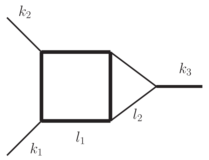
(b) $m_{1}\not=0$, $m_{2}=0$

(c) $m_{1}\not=0$, $m_{2}\not=0$

Figure 1: Two-loop box triangle diagrams

We consider different mass configurations:

• $m_{1}=m_{2}=0$. In this case, the Baikov polynomial with maximal cut $z_{1}=\ldots=z_{6}=0$ is

  $$F=-\frac{1}{4}z_{7}^{2}\,.$$ (32)

  A generic integrand $z_{7}^{k}/(z_{1}\ldots z_{6})$, $k\in\mathbb{N}_{0}$, on the maximal cut reads,

  $$I[1,1,1,1,1,1,-k]\big{|}_{\rm m.c.}=\frac{2^{D-4}}{\pi^{3}\Gamma(D-3)}\frac{1}{8s^{2}}\int_{\Omega}dz_{7}\big{(}-\frac{1}{4}z_{7}^{2}\big{)}^{(D-5)/2}z_{7}^{k}\,.$$ (33)

  Note that

  $$d\bigg{(}\frac{1}{D-4+k}\big{(}-\frac{1}{4}z_{7}^{2}\big{)}^{(D-5)/2}z_{7}^{k+1}\bigg{)}=\big{(}-\frac{1}{4}z_{7}^{2}\big{)}^{(D-5)/2}z_{7}^{k}dz_{7}\,,$$ (34)

  so the integrand of (33) is a polynomial-valued total derivative. Hence

  $$I[1,1,1,1,1,1,-k]\big{|}_{\rm m.c.}=0\,,\quad k\in\mathbb{N}_{0}\,.$$ (35)

  The $D$-dimensional maximal cut vanishes and this implies that the massless box-triangle integral is reducible (to integrals with fewer propagators).

• $m_{1}\not=0$, $m_{2}=0$. In this case, the Baikov polynomial with maximal cut $z_{1}=\ldots=z_{6}=0$ is

  $$F=\frac{z_{7}(4m_{1}^{2}s+4m_{1}^{2}z_{7}-sz_{7})}{4s}\,.$$ (36)

  To simplify the expression, we may redefine the ISP as

  $$\tilde{D}_{7}=z\equiv\frac{4m_{1}^{2}-s}{4m_{1}^{2}s}z_{7}+\frac{1}{2}=\frac{4m_{1}^{2}-s}{4m_{1}^{2}s}(l_{2}+p_{1})^{2}+\frac{1}{2}\,,$$ (37)

  $$\tilde{I}[a_{1},a_{2},a_{3},a_{4},a_{5},a_{6},-k]=\int\frac{d^{D}l_{1}}{\pi^{D/2}}\frac{d^{D}l_{2}}{\pi^{D/2}}\frac{\tilde{D}_{7}^{k}}{D_{1}^{a_{1}}D_{2}^{a_{2}}D_{3}^{a_{3}}D_{4}^{a_{4}}D_{5}^{a_{5}}D_{6}^{a_{6}}}\,.$$ (38)

  Then

  $$F=\frac{4s^{2}x^{2}}{4x-1}(z-\frac{1}{2})(z+\frac{1}{2})\,,$$ (39)

  where $x=m_{1}^{2}/s$.

  We consider the kinematic region $s<4m^{2}$ ($x>1/4$). The $D$-dimensional cut reads

  $$\tilde{I}[1,1,1,1,1,1,-k]\big{|}_{\rm m.c.}=\frac{2^{D-4}}{\pi^{3}\Gamma(D-3)}\frac{x}{2s(4x-1)}\int_{\Omega}dzF^{(D-5)/2}z^{k}\,.$$ (40)

  When $x>1/4$, $\Omega=\Omega_{1}\cup\Omega_{2}$, where $\Omega_{1}=(1/2,\infty)$ and $\Omega_{2}=(-\infty,-1/2)$. The integration (40) over $\Omega_{1}$ is

  $$\tilde{I}[1,1,1,1,1,1,-k]\big{|}_{\rm m.c.}^{(1)}=\frac{s^{D-6}x^{D-4}(4x-1)^{\frac{3}{2}-\frac{D}{2}}}{2^{k+3}\pi^{\frac{5}{2}}}\frac{\Gamma(\frac{4-D-k}{2})}{\Gamma(\frac{D}{2}-1)\Gamma(\frac{1}{2}-\frac{k}{2})}\,,$$ (41)

  and similarly over the region $\Omega_{2}$,

  $$\tilde{I}[1,1,1,1,1,1,-k]\big{|}_{\rm m.c.}^{(2)}=(-1)^{k}\tilde{I}[1,1,1,1,1,1,-k]\big{|}_{\rm m.c.}^{(1)}\,.$$ (42)

  These integrals are convergent when ${\rm Re}(D)>3$ and $k+{\rm Re}(D)<4$. We use (41) as an analytic continuation for generic values of $D$ and $k$. Note that because of the factor $1/\Gamma(\frac{1}{2}-\frac{k}{2})$, $\tilde{I}[1,1,1,1,1,1,-k]\big{|}_{\rm m.c.}^{(1)}=0$ for positive odd $k$. So for $k\in N_{0}$,

  $$\tilde{I}[1,1,1,1,1,1,-k]\big{|}_{\rm m.c.}^{(1)}=\tilde{I}[1,1,1,1,1,1,-k]\big{|}_{\rm m.c.}^{(2)}\,,\quad k\in N_{0}\,.$$ (43)

  Hence we define the $D$-dimensional maximal cut as

  $$\tilde{I}[1,1,1,1,1,1,-k]\big{|}_{\rm m.c.}\equiv\tilde{I}[1,1,1,1,1,1,-k]\big{|}_{\rm m.c.}^{(1)}\,.$$ (44)

  By expression (44), we find that

  $$\tilde{I}[1,1,1,1,1,1,-2]\big{|}_{\rm m.c.} = \frac{1}{4(D-2)}\tilde{I}[1,1,1,1,1,1,0]\big{|}_{\rm m.c.}\,,$$ (45)

  $$\tilde{I}[1,1,1,1,1,1,-4]\big{|}_{\rm m.c.} = \frac{3}{16D(D-2)}\tilde{I}[1,1,1,1,1,1,0]\big{|}_{\rm m.c.}\,,$$ (46)

  $$\tilde{I}[1,1,1,1,1,1,-6]\big{|}_{\rm m.c.} = \frac{15}{64(D+2)D(D-2)}\tilde{I}[1,1,1,1,1,1,0]\big{|}_{\rm m.c.}\,.$$ (47)

  They imply the Feynman integral relations,

  $$\tilde{I}[1,1,1,1,1,1,-2] = \frac{1}{4(D-2)}\tilde{I}[1,1,1,1,1,1,0]+\ldots\,,$$ (48)

  $$\tilde{I}[1,1,1,1,1,1,-4] = \frac{3}{16D(D-2)}\tilde{I}[1,1,1,1,1,1,0]+\ldots\,,$$ (49)

  $$\tilde{I}[1,1,1,1,1,1,-6] = \frac{15}{64(D+2)D(D-2)}\tilde{I}[1,1,1,1,1,1,0]+\ldots\,,$$ (50)

  where $\ldots$ stands for integrals with fewer propagators. These identities agree with IBP output from FIRE Smirnov:2005ky ; Smirnov:2006tz ; Smirnov:2008iw ; Smirnov:2014hma , LiteRed Lee:2012cn ; Lee:2013mka , and Azurite Georgoudis:2016wff .

  The expression (44) can also be used for deriving the dimension shift identity,

  $$\tilde{I}[1,1,1,1,1,1,0](D+2)\big{|}_{\rm m.c.}=-\frac{4m^{4}s}{(D-2)^{2}(4m^{2}-s)}\tilde{I}[1,1,1,1,1,1,0](D)\big{|}_{\rm m.c.}\,,$$ (51)

  which means the dimension shift identity on the maximal cut.

  It is also interesting to study the differential equation on the maximal cut,

  $$\frac{\partial}{\partial x}\tilde{I}[1,1,1,1,1,1,0]=\bigg{(}-2\frac{D-3}{4x-1}+\frac{D-4}{x}\bigg{)}\tilde{I}[1,1,1,1,1,1,0]+\ldots\,,$$ (52)

  where $\ldots$ stands for integrals with fewer propagators. Explicitly, we see that the $D$-dimensional cut $\tilde{I}[1,1,1,1,1,1,0]\big{|}_{\rm m.c.}$ solves the maximal cut part of this equation.

  We can expand the $D$-dimensional maximal cut in $\epsilon$ $(D=4-2\epsilon)$,

  $$\tilde{I}[1,1,1,1,1,1,0]\big{|}_{\rm m.c.}=\frac{1}{8\pi^{3}s^{2}\sqrt{4x-1}\epsilon}+\frac{-2\log(s)-2\log(x)+\log(4x-1)-2\gamma}{8\pi^{3}s^{2}\sqrt{4x-1}}$$

  $$+\frac{\epsilon}{16\pi^{3}s^{2}\sqrt{4x-1}}\bigg{(}8\log(s)\log(x)-4\log(s)\log(4x-1)+4\log^{2}(s)+8\gamma\log(s)+4\log^{2}(x)$$

  $$+\log^{2}(4x-1)+8\gamma\log(x)-4\log(x)\log(4x-1)-4\gamma\log(4x-1)+4\gamma^{2}\bigg{)}+O\left(\epsilon^{2}\right)\,,$$ (53)

  where $\gamma$ is the Euler-Mascheroni constant. From the leading coefficient in $\epsilon$, we see that we may redefine the integral,

  $$J\equiv s^{2}\sqrt{4x-1}\tilde{I}[1,1,1,1,1,1,0]\,,$$ (54)

  such that the differential equation on the maximal cut has the $\epsilon$ form,

  $$\frac{\partial}{\partial x}J=\epsilon\frac{2-4x}{(4x-1)x}J+\ldots,$$ (55)

  where $\ldots$ stands for integrals with fewer propagators.

• $m_{1}\not=0$, $m_{2}\not=0$. Define $x_{1}=m_{1}^{2}/s$ and $x_{2}=m_{2}^{2}/s$. Following similar steps as in the previous case, we define

  $$\tilde{D}_{7}=z\equiv\frac{4m_{1}^{2}-s}{4m_{1}^{2}s}z_{7}+\frac{1}{2}-\frac{m_{2}^{2}}{s}=\frac{4m_{1}^{2}-s}{4m_{1}^{2}s}(l_{2}+p_{1})^{2}+\frac{1}{2}-\frac{m_{2}^{2}}{s}\,,$$ (56)

  $$\tilde{I}[a_{1},a_{2},a_{3},a_{4},a_{5},a_{6},-k]=\int\frac{d^{D}l_{1}}{\pi^{D/2}}\frac{d^{D}l_{2}}{\pi^{D/2}}\frac{\tilde{D}_{7}^{k}}{D_{1}^{a_{1}}D_{2}^{a_{2}}D_{3}^{a_{3}}D_{4}^{a_{4}}D_{5}^{a_{5}}D_{6}^{a_{6}}}\,.$$ (57)

  We find that the $D$-dimensional maximal cut is

  $$\tilde{I}[a_{1},a_{2},a_{3},a_{4},a_{5},a_{6},-k]\big{|}_{\rm m.c.}$$

  $$=\frac{s^{D-6}x_{1}^{D-4}(4x_{1}-1)^{\frac{3}{2}-\frac{D}{2}}(1-4x_{2}+\frac{x_{2}^{2}}{x_{1}})^{\frac{D+k-4}{2}}}{2^{k+2}\pi^{\frac{5}{2}}}\frac{\Gamma(\frac{4-D-k}{2})}{\Gamma(\frac{D}{2}-1)\Gamma(\frac{1}{2}-\frac{k}{2})}\,.$$ (58)

  Again, we can use it to study the IBPs, dimension shift identities, differential equations and $\epsilon$-form, on the maximal cut.

5 Planar maximal cuts with two ISPs

Now we consider $D$-dimensional maximal cuts with two ISPs. In this case, the integral regions become less trivial and we can investigate each region seperately to get a complete set of $D$-dimensional maximal cut functions in kinematic variables.

5.1 Massless sunset

Figure 2: The massless sunset diagram.All momenta flow to the right.

As a warm-up, consider the sunset diagram with massless internal propagators, see figure 2. We have the inverse propagators

$$D_{1}=l_{1}^{2}\,,\quad D_{2}=l_{2}^{2}\,,\quad D_{3}=(l_{1}+l_{2}-k)^{2}\,.$$ (59)

There are two ISPs, which we may choose to be

$$D_{4}=(l_{1}+k)^{2}-2s\,,\quad D_{5}=(l_{2}+k)^{2}-2s\,,$$ (60)

where $s=k^{2}$. Our object of interest is the integral

$$I[a_{1},a_{2},a_{3},-a_{4},-a_{5}]\equiv\int\limits\frac{d^{D}l_{1}}{\pi^{D/2}}\frac{d^{D}l_{2}}{\pi^{D/2}}\frac{D_{4}^{a_{4}}D_{5}^{a_{5}}}{D_{1}^{a_{1}}D_{2}^{a_{2}}D_{3}^{a_{3}}}\,.$$ (61)

Taking the Baikov variables to be $z_{i}=D_{i}$, equation (61) becomes

$$I[a_{1},a_{2},a_{3},-a_{4},-a_{5}]=\frac{1}{s}\frac{2^{D-4}\pi^{D-2}}{\Gamma(D-2)}\int\limits_{\Omega}\left(\prod\limits_{i=1}^{5}dz_{i}\right)F^{\frac{D-4}{2}}\frac{z_{4}^{a_{4}}z_{5}^{a_{5}}}{z_{1}^{a_{1}}z_{2}^{a_{2}}z_{3}^{a_{3}}}\,,$$ (62)

where the integration region $\Omega$ is defined by $F(z)\geq 0$. On the maximal cut the Baikov polynomial is

$$F=\frac{1}{4s}z_{4}z_{5}(s+z_{4}+z_{5})\,,$$ (63)

which we can simplify by rescaling the Baikov variables to

$$x=\frac{z_{4}}{s}\,,\quad y=\frac{z_{5}}{s}\,.$$ (64)

This gives

$$F=xy(1+x+y)\,,$$ (65)

and our integral of interest on the maximal cut then reads

$$J[a,b]\big{|}_{\rm m.c.}^{(\Omega)}=s^{2}\left(\frac{s^{2}}{4}\right)^{\frac{D-4}{2}}\frac{2^{D-4}\pi^{D-2}}{\Gamma(D-2)}s^{a+b}\int\limits_{\Omega}F^{\frac{D-4}{2}}x^{a}y^{b}dxdy\,,$$ (66)

where we have defined the shorthand $J[a,b]\equiv I[1,1,1,-a,-b]$ for notational convenience. The integration splits into four regions,

• $x,y>0$,

• $x>0$, $y<-(1+x)$,

• $x<-(1+y)$, $y>0$,

• $-1<x<0$, $-(1+x)<y<0$.

These regions are shown schematically in figure 3.

Figure 3: Subregions for the integration of the sunset diagram on the maximal cut.

The integration in each of the regions can now be carried out explicitly to give

$$I_{\text{I}} =\int\limits_{0}^{\infty}\int\limits_{0}^{\infty}x^{a}y^{b}(xy(1+x+y))^{\frac{D-4}{2}}dydx$$

$$=\frac{\Gamma(4-a-b-3D/2)\Gamma(-1+a+D/2)\Gamma(-1+b+D/2)}{\Gamma(2-D/2)}\,,$$

$$I_{\text{II}} =\int\limits_{0}^{\infty}\int\limits_{-\infty}^{-(1+x)}x^{a}y^{b}(xy(1+x+y))^{\frac{D-4}{2}}dydx$$

$$=(-1)^{b}\frac{\Gamma(4-a-b-3D/2)\Gamma(-1+a+D/2)\Gamma(-1+D/2)}{\Gamma(2-b-D/2)}\,,$$

$$I_{\text{III}} =\int\limits_{0}^{\infty}\int\limits_{-\infty}^{-(1+y)}x^{a}y^{b}(xy(1+x+y))^{\frac{D-4}{2}}dxdy$$

$$=(-1)^{a}\frac{\Gamma(4-a-b-3D/2)\Gamma(-1+D/2)\Gamma(-1+b+D/2)}{\Gamma(2-a-D/2)}\,,$$

$$I_{\text{IV}} =\int\limits_{-1}^{0}\int\limits_{-(1+x)}^{0}x^{a}y^{b}(xy(1+x+y))^{\frac{D-4}{2}}dydx$$

$$=\frac{(-1)^{1+a+b}\pi}{\sin(D\pi/2)}\,\frac{\Gamma(-1+a+D/2)\Gamma(-1+b+D/2)}{\Gamma(2-D/2)\Gamma(-3+a+b+3D/2)}\,.$$

Note that the integrals only converge when certain restrictions on $a$, $b$, and $D$ are satisfied, but we drop those as we are interested in the analytic continuation anyway. Assuming $a$ and $b$ to be non-negative integers, it follows from the reflection property of the gamma function, $\sin(\pi z)\Gamma(1-z)\Gamma(z)=\pi$, that

$$I_{\text{I}}=I_{\text{II}}=I_{\text{III}}\,,\quad I_{\text{IV}}=(1+2\cos(D\pi))I_{\text{I}}\,.$$ (67)

So there is only one linearly independent function. (Here the coefficient field is set to be the meromorphic function field of $D$.) We thus set the $D$-dimensional maximal cut as the integration over the region I,

$$\begin{aligned} J[a,b]\big{|}_{\rm m.c.}&=\frac{\pi^{D-2}}{\Gamma(D-2)}s^{a+b+D-2}\\ &\quad\times\frac{\Gamma(4-a-b-3D/2)\Gamma(-1+a+D/2)\Gamma(-1+b+D/2)}{\Gamma(2-D/2)}\,.\end{aligned}$$ (68)

If we introduce the descending factorial

$$(z)^{(\underline{r})}\equiv\frac{\Gamma(z+1)}{\Gamma(z-r+1)}=z(z-1)\cdots(z-r+1),$$ (69)

which is related to the Pochhammer symbol (26) by

$$(z)_{r}=(-1)^{r}(-z)^{(\underline{r})}\,,$$ (70)

it is straightforward to see that

$$J[a,b]\big{|}_{\rm m.c.}=J[0,0]\big{|}_{\rm m.c.}\,s^{a+b}\frac{\left(-1+\frac{D}{2}\right)_{a}\left(-1+\frac{D}{2}\right)_{b}}{\left(3-\frac{3D}{2}\right)^{(\underline{a+b})}}\,.$$ (71)

For $a$ and $b$ non-negative integers the last factor evaluates to a rational function in $D$, as one would expect. Equation (71) agrees with IBPs found with FIRE Smirnov:2005ky ; Smirnov:2006tz ; Smirnov:2008iw ; Smirnov:2014hma , LiteRed Lee:2012cn ; Lee:2013mka , and Azurite Georgoudis:2016wff .

In a similar way we readily find the dimension shift identity,

$$\begin{aligned} J[0,0]\big{|}_{\rm m.c.}(D+2)=-\,s^{2}\pi^{2}\frac{(-1+D/2)(-1+D/2)}{2(1-3D/2)_{3}(D-1)}\times J[0,0]\big{|}_{\rm m.c.}(D)\,.\end{aligned}$$ (72)

The differential equation for $J[0,0]\big{|}_{\rm m.c.}$ is simple,

$$\frac{\partial}{\partial s}J[0,0]\big{|}_{\rm m.c.}=\frac{D-2}{s}J[0,0]\big{|}_{\rm m.c.}\,,$$ (73)

and is immediately in $\epsilon$-form if we specialize to $D=2-2\epsilon$.

5.2 Massless double box

The diagram is shown in figure 4.

Figure 4: Massless double box diagram. This graph is produced by the package Azurite Georgoudis:2016wff .

The inverse propagators are

$$D_{1}=l_{1}^{2}\,,\quad D_{2}=(l_{1}-k_{1})^{2}\,,\quad D_{3}=(l_{1}-k_{1}-k_{2})^{2}\,,$$

$$D_{4}=(l_{2}+k_{1}+k_{2})^{2}\,,\quad D_{5}=(l_{2}-k_{4})^{2}\,,\quad D_{6}=l_{2}^{2}\,,\quad D_{7}=(l_{1}+l_{2})^{2}\,,$$ (74)

and the external momenta satisfy $k_{1}^{2}=k_{2}^{2}=k_{4}^{2}=0$, $(k_{1}+k_{2})^{2}=s$ and $(k_{1}+k_{4})^{2}=t$. We define $\chi=t/s$. There are $2(4-1)+2(2+1)/2=9$ scalar products in loop momenta, hence we have two ISPs,

$$D_{8}=(l_{1}+k_{4})^{2}\,,\quad D_{9}=(l_{2}+k_{1})^{2}\,.$$ (75)

The integrals under consideration are

$$I[n_{1},n_{2},\ldots,n_{7},-a,-b]\equiv\int\frac{d^{D}l_{1}}{\pi^{D/2}}\frac{d^{D}l_{2}}{\pi^{D/2}}\frac{D_{8}^{a}D_{9}^{b}}{D_{1}^{n_{1}}D_{2}^{n_{2}}\ldots D_{7}^{n_{7}}}\,.$$ (76)

To simplify notation, define $J[a,b]\equiv I[1,1,1,1,1,1,1,-a,-b]$. Again we hide the argument $D$, except for the discussion of dimensional shift identities.

The Baikov polynomial on the maximal cut is

$$F=\frac{z_{8}z_{9}\left(s^{2}\chi-sz_{8}-sz_{9}-z_{8}z_{9}\right)}{4s^{2}\chi(\chi+1)}\,.$$ (77)

The maximal cut of $J[a,b]$ can be calculated by the integration of $F^{(D-6)/2}z_{8}^{a}z_{9}^{b}$. Consider the kinematic condition $s>0,\chi>0$. The integration region defined by $F\geq 0$ splits into four subregions:

• $z_{8}>0$, $z_{9}>0$, $s^{2}\chi-sz_{8}-sz_{9}-z_{8}z_{9}>0$,

• $z_{8}>0$, $z_{9}<0$, $s^{2}\chi-sz_{8}-sz_{9}-z_{8}z_{9}<0$,

• $z_{8}<0$, $z_{9}>0$, $s^{2}\chi-sz_{8}-sz_{9}-z_{8}z_{9}<0$,

• $z_{8}<0$, $z_{9}<0$, $s^{2}\chi-sz_{8}-sz_{9}-z_{8}z_{9}>0$,

which are shown in figure 5 as the blue area. It is clear that on the four subregions the conditions $\mu_{11}(z)\geq 0$ and $\mu_{22}(z)\geq 0$ are satisfied.

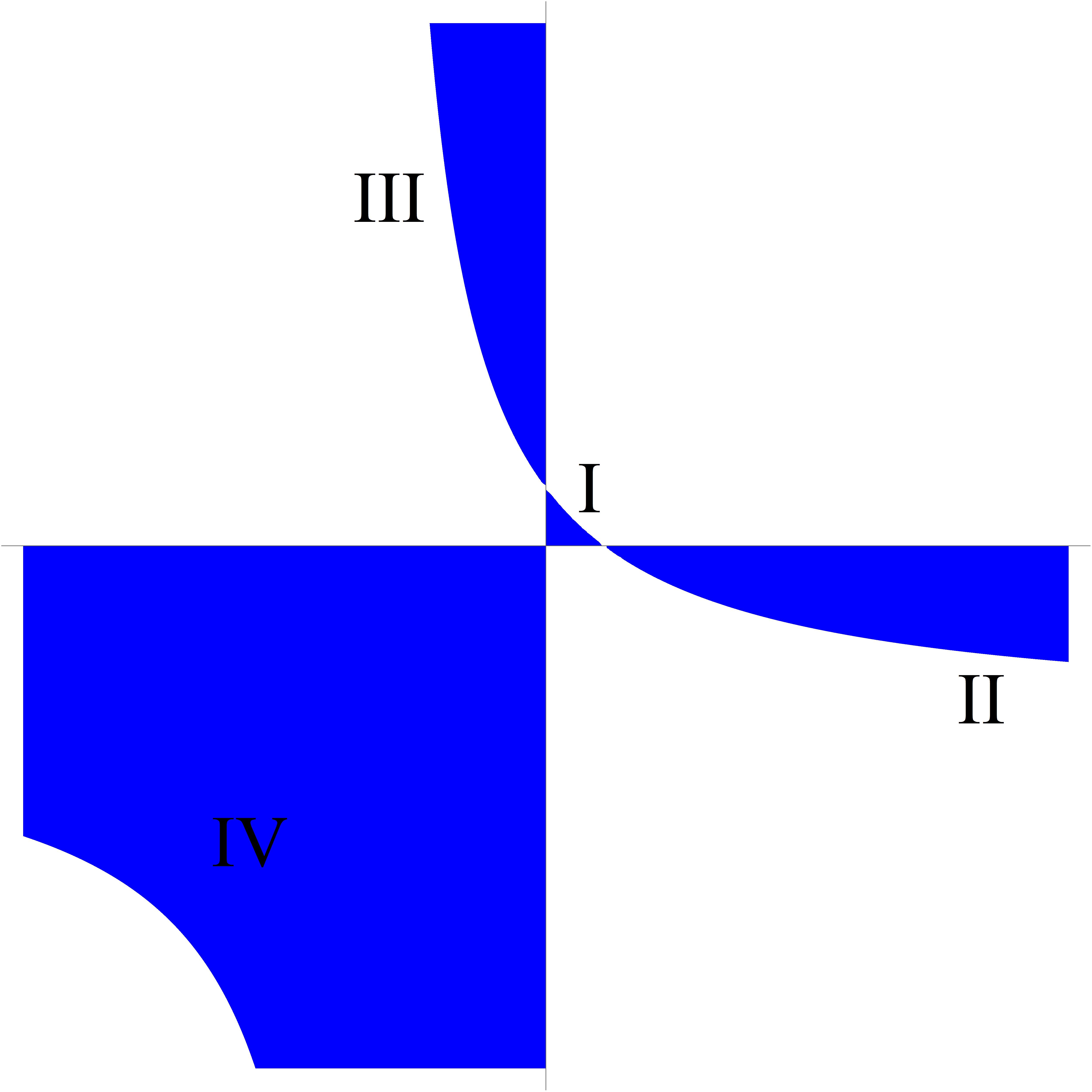
Figure 5: Subregions for the integration of the massless double box diagram on the maximal cut. This plot is for the kinematic configuration, $s=1$ and $\chi=1/3$. The two axes are the ISPs, $z_{8}$ and $z_{9}$. These subregions are symmetric under the flip of two axes.

The integrations over the first three subregions are straightforward, while the integration over the fourth subregion needs careful further splitting. The integration over $\Omega_{\text{I}}$ reads,

$$J[a,b]\big{|}_{\rm m.c.}^{\text{(I)}} =\frac{2^{D-10}}{\pi^{4}st\Gamma(D-4)(s+t)}\int_{0}^{\chi s}dz_{8}\int_{0}^{\frac{s(\chi s-z_{8})}{s+z_{8}}}dz_{9}F^{\frac{D-6}{2}}z_{8}^{a}z_{9}^{b}$$

$$=\frac{\Gamma\left(\frac{D}{2}-2\right)\Gamma\left(a+\frac{D}{2}-2\right)\Gamma\left(b+\frac{D}{2}-2\right)s^{a+b+D-7}\chi^{a+b+D-5}\,}{16\pi^{4}\Gamma(D-4)}$$

$$\times\ _{2}\tilde{F}_{1}\left(a+D-4,b+D-4;a+b+\frac{3D}{2}-6;-\chi\right)\,,$$ (78)

where ${}_{2}\tilde{F}_{1}$ is the regularized hypergeometric function, ${}_{2}\tilde{F}_{1}(\alpha,\beta,\gamma,z)=\,_{2}F_{1}(\alpha,\beta,\gamma,z)/\Gamma(\gamma)$. This result is to be understood as an analytic continuation over $D$, $a$ and $b$.

Similarly the second integration over $\Omega_{\text{II}}$ gives

$$J[a,b]\big{|}_{\rm m.c.}^{\text{(II)}} =\frac{(-1)^{b}\Gamma\left(\frac{D}{2}-2\right)\Gamma(-a-D+5)\Gamma\left(b+\frac{D}{2}-2\right)s^{a+b+D-7}\chi^{a+\frac{D}{2}-3}(\chi+1)^{2-\frac{D}{2}}}{16\pi^{4}\Gamma(D-4)}$$

$$\times\,_{2}\tilde{F}_{1}\left(-a-D+5,b+\frac{D}{2}-2;-a+b+1;-\frac{1}{\chi}\right)\,.$$ (79)

Although apparently this expression does not look symmetric in $a$ and $b$, after a hypergeometric function transformation, the symmetry is manifest:

$$J[a,b]\big{|}_{\rm m.c.}^{\text{(II)}} =-\frac{(-1)^{a+b}\chi^{2-\frac{D}{2}}\sin(\pi D)\Gamma\left(\frac{D}{2}-2\right)\Gamma(-a-D+5)\Gamma(-b-D+5)s^{a+b+D-7}}{16\pi^{4}\Gamma(D-4)\sin\left(\frac{3\pi D}{2}\right)}$$

$$\times\,_{2}\tilde{F}_{1}\left(-a-\frac{D}{2}+3,-b-\frac{D}{2}+3;-a-b-\frac{3D}{2}+8;-\chi\right)$$

$$+\frac{\Gamma\left(\frac{D}{2}-2\right)\Gamma\left(a+\frac{D}{2}-2\right)\Gamma\left(b+\frac{D}{2}-2\right)s^{a+b+D-7}\chi^{a+b+D-5}\,}{16\pi^{4}\Gamma(D-4)\big{(}1+2\cos(\pi D)\big{)}}$$

$$\times\ _{2}\tilde{F}_{1}\left(a+D-4,b+D-4;a+b+\frac{3D}{2}-6;-\chi\right)\,.$$ (80)

The integration over $\Omega_{\text{III}}$ gives

$$J[a,b]\big{|}_{\rm m.c.}^{\text{(III)}}=J[a,b]\big{|}_{\rm m.c.}^{\text{(II)}}\,.$$ (81)

Finally, using the transformation identities of hypergeometric functions, the integration over $\Omega_{\text{IV}}$ is

$$J[a,b]\big{|}_{\rm m.c.}^{\text{(IV)}}=J[a,b]\big{|}_{\rm m.c.}^{\text{(I)}}-2\cos(\pi D)J[a,b]\big{|}_{\rm m.c.}^{\text{(II)}}\,.$$ (82)

Since the integrations over region III and IV are dependent of the integrations over the first two regions, we can define the $D$-dimensional maximal cut as a list of two functions,

$$J[a,b]\big{|}_{\rm m.c.}\equiv\bigg{(}J[a,b]\big{|}_{\rm m.c.}^{\text{(I)}},\ J[a,b]\big{|}_{\rm m.c.}^{\text{(II)}}\bigg{)}\,.$$ (83)

The independence of $J[a,b]\big{|}_{\rm m.c.}^{\text{(I)}}$ and $J[a,b]\big{|}_{\rm m.c.}^{\text{(II)}}$ will be discussed later on.

Then by Gauss’ contiguous relations of $\,{}_{2}F_{1}$ functions, we see that for integer-valued $a$ and $b$’s, $J[a,b]\big{|}_{\rm m.c.}^{\text{(I)}}$’s are linearly generated by $J[0,0]\big{|}_{\rm m.c.}^{\text{(I)}}$, $J[1,0]\big{|}_{\rm m.c.}^{\text{(I)}}$, in the field of rational functions of $D$, $s$ and $\chi$. Similarly, $J[a,b]\big{|}_{\rm m.c.}^{\text{(II)}}$’s are linearly generated by $J[0,0]\big{|}_{\rm m.c.}^{\text{(II)}}$, $J[1,0]\big{|}_{\rm m.c.}^{\text{(II)}}$. Explicitly, we can check that Gauss’ contiguous relations of all regional integrations, $J[a,b]\big{|}_{\rm m.c.}^{(i)}$, $i=$I, II, III, IV, provide the maximal cut $D$-dimensional IBPs,

$$J[1,1]\big{|}_{\rm m.c.}^{(i)} =\frac{1}{2}s^{2}J[0,0]\big{|}_{\rm m.c.}^{(i)}-\frac{3}{2}sJ[1,0]\big{|}_{\rm m.c.}^{(i)}\,,$$

$$J[2,0]\big{|}_{\rm m.c.}^{(i)} =\frac{(D-4)s^{2}\chi}{2(D-3)}J[0,0]\big{|}_{\rm m.c.}^{(i)}-\frac{(3D-2\chi-12)s}{2(D-3)}J[1,0]\big{|}_{\rm m.c.}^{(i)}\,,$$

$$J[2,1]\big{|}_{\rm m.c.}^{(i)} =\frac{s^{2}(2D\chi+9D-8\chi-30)}{4(D-3)}J[1,0]\big{|}_{\rm m.c.}^{(i)}-\frac{(3D-10)s^{3}\chi}{4(D-3)}J[0,0]\big{|}_{\rm m.c.}^{(i)}\,.$$ (84)

These identities agree with the IBP output from FIRE Smirnov:2005ky ; Smirnov:2006tz ; Smirnov:2008iw ; Smirnov:2014hma , LiteRed Lee:2012cn ; Lee:2013mka , and Azurite Georgoudis:2016wff . We conclude that the function relations for $J[a,b]\big{|}_{\rm m.c.}$ provide the IBPs on the maximal cuts.

Gauss’ contiguous relations also imply dimension shift identities on the maximal cut. For example, for $i=$I, II, III, IV,

$$J[0,0]\big{|}_{\rm m.c.}^{(i)}(D+2)=\frac{s^{2}(2(D-3)\chi+3d-10)}{8(D-3)^{3}(\chi+1)}J[0,0]\big{|}_{\rm m.c.}^{(i)}(D)$$

$$-\frac{s(8D\chi+9D-26\chi-30)}{8(D-3)^{3}\chi(\chi+1)}J[1,0]\big{|}_{\rm m.c.}^{(i)}(D)\,.$$ (85)

Note that the $\cos(\pi D)$ factor in the region (82) does not affect dimension shift identities, since it is invariant under $D\to D+2$. We also remark that it is well-known that the solutions of recursive relations for the dimension shift identities may consist of hypergeometric functions Lee:2012te .

We know that the two master integrals of the double box topology satisfy the differential equation on the maximal cut,

$$\frac{\partial}{\partial\chi}\left(\begin{array}[]{c}J[0,0]\\ J[1,0]\end{array}\right)=\left(\begin{array}[]{cc}\frac{D-\chi-5}{\chi(\chi+1)}&\frac{D-4}{s\chi(\chi+1)}\\ \frac{(D-4)s}{2(\chi+1)}&-\frac{D-4}{2\chi(\chi+1)}\\ \end{array}\right)\left(\begin{array}[]{c}J[0,0]\\ J[1,0]\end{array}\right)+\ldots\,,$$ (86)

where $\ldots$ stands for integrals with fewer propagators. We verify that for $i=$ I, II, III, IV, $(J[0,0]\big{|}_{\rm m.c.}^{(i)},J[1,0]\big{|}_{\rm m.c.}^{(i)})^{\rm T}$ solves (86). The maximal cut functions $J[a,b]\big{|}_{\rm m.c.}$ with $(a,b)=(0,0)$, $(1,0)$ form the fundamental solutions of (86),

$$S=\left(\begin{array}[]{c}J[0,0]\big{|}_{\rm m.c.}\\ J[1,0]\big{|}_{\rm m.c.}\end{array}\right)\,,$$

because the Wronskian is nonzero,

$$\det S\propto\chi^{\frac{d}{2}-3}(\chi+1)^{2-\frac{d}{2}}\,.$$ (87)

This justifies the definition of (83) since $J[a,b]\big{|}_{\rm m.c.}^{\text{I}}$ and $J[a,b]\big{|}_{\rm m.c.}^{\text{II}}$ are independent functions in $\chi$.

Finally we check the matrix $S$ in the $D\to 4$ limit and extract the leading coefficients in $\epsilon$. Using the HypExp package Huber:2005yg ; Huber:2007dx , the result is

$$T=\left(\begin{array}[]{cc}\frac{3}{4\pi^{4}s^{3}\chi}&\frac{1}{4\pi^{4}s^{3}\chi}\\ \frac{1}{4\pi^{4}s^{2}}&0\\ \end{array}\right)\,.$$ (88)

From the leading coefficients in $T$ and a suitable linear combination, we may define the transformation matrix

$$\tilde{T}=T\left(\begin{array}[]{cc}0&1\\ 1&-3\end{array}\right)\cdot 4\pi^{4}\,.$$ (91)

Hence we redefine the master integrals as

$$\tilde{J}[0,0]=s^{3}\chi J[0,0]\,,\quad\tilde{J}[1,0]=s^{2}\chi J[1,0]\,,$$ (92)

and the differential equation on the maximal cut (86) turns into the $\epsilon$-form:

$$\frac{\partial}{\partial\chi}\left(\begin{array}[]{c}\tilde{J}[0,0]\\ \tilde{J}[1,0]\\ \end{array}\right)=(D-4)\left(\begin{array}[]{cc}\frac{1}{\chi(\chi+1)}&\frac{1}{\chi+1}\\ \frac{1}{2\chi(\chi+1)}&-\frac{1}{2\chi(\chi+1)}\\ \end{array}\right)\left(\begin{array}[]{c}\tilde{J}[0,0]\\ \tilde{J}[1,0]\\ \end{array}\right)+\ldots\,.$$ (93)

5.3 Double box with one massive leg

We can use the same method to consider the maximal cut of the double box with one massive external leg. The Feynman integral has the same inverse propagators (29), and the kinematic conditions are $k_{1}^{2}=m_{1}^{2}$, $k_{2}^{2}=k_{3}^{2}=k_{4}^{2}=0$. The two ISP are $D_{8}=(l_{1}+k_{4})^{2}$, $D_{9}=(l_{2}+k_{1})^{2}$ and the diagram is shown in figure 6.

Figure 6: Double box diagram with one external massive leg. This graph is produced by the package Azurite .

Define $\chi=t/s$, $\kappa=m_{1}^{2}/s$, $x=z_{8}/s$ and $y=z_{9}/s$. The Baikov polynomial on the maximal cut reads

$$F=\frac{s^{2}xy(\chi+\kappa x-xy-x-y)}{4\chi(-\kappa+\chi+1)}\,.$$ (94)

Consider the kinematic region $s>0$, $\chi>0$ and $\chi+1-\kappa>0$. Again, the integration region defined by $F\geq 0$ splits into four subregions:

• $x>0$, $y>0$, $\chi+\kappa x-xy-x-y>0$,

• $x>0$, $y<0$, $\chi+\kappa x-xy-x-y<0$,

• $x<0$, $y>0$, $\chi+\kappa x-xy-x-y<0$,

• $x<0$, $y<0$, $\chi+\kappa x-xy-x-y>0$.

The subregions are shown in figure 9. On the four subregions the conditions $\mu_{11}(z)\geq 0$ and $\mu_{22}(z)\geq 0$ are satisfied.

Figure 7: Subregions for the integration of the double box diagram with one external massive leg on the maximal cut. The plot is for the kinematic configuration $s=1$, $\chi=1/3$ and $\kappa=1/2$. On the horizontal and vertical axis we have $x$ and $y$, respectively. Note that the subregions are not symmetric under a flip of the axes.

The integrals under consideration are

$$I[n_{1},n_{2},\ldots,n_{7},-a,-b]\equiv\int\frac{d^{D}l_{1}}{\pi^{D/2}}\frac{d^{D}l_{2}}{\pi^{D/2}}\frac{D_{8}^{a}D_{9}^{b}}{D_{1}^{n_{1}}D_{2}^{n_{2}}\ldots D_{7}^{n_{7}}}\,.$$ (95)

Again we define $J[a,b]\equiv I[1,1,1,1,1,1,1,-a,-b]$. The integration over $\Omega_{\text{I}}$ reads

$$J[a,b]\big{|}_{\rm m.c.}^{\text{(I)}} =\frac{\Gamma\left(\frac{D}{2}-2\right)\Gamma\left(a+\frac{D}{2}-2\right)\Gamma\left(b+\frac{D}{2}-2\right)s^{a+b-7}\chi^{a+b+d-5}\left(\frac{1}{1-\kappa}\right)^{a+d-4}}{16\pi^{4}\chi^{5}\Gamma(D-4)}$$

$$\times\,_{2}\tilde{F}_{1}\left(a+D-4,b+D-4;a+b+\frac{3D}{2}-6;\frac{\chi}{\kappa-1}\right)\,.$$ (96)

while the integration over $\Omega_{\text{II}}$ reads

$$J[a,b]\big{|}_{\rm m.c.}^{\text{(II)}} =\frac{(-1)^{b}(1-\kappa)^{-a+b}\Gamma\left(\frac{D}{2}-2\right)\chi^{a+\frac{D}{2}-3}\Gamma(-a-D+5)\Gamma\left(b+\frac{D}{2}-2\right)s^{a+b+D-7}}{16\pi^{4}\Gamma(D-4)}$$

$$\times(-\kappa+\chi+1)^{2-\frac{D}{2}}\,_{2}\tilde{F}_{1}\left(-a-D+5,b+\frac{D}{2}-2;-a+b+1;\frac{\kappa-1}{\chi}\right)\,.$$ (97)

Similar to the massless case, the integrations over $\Omega_{\text{III}}$ and $\Omega_{\text{IV}}$ are related to the previous two integrals through

$$J[a,b]\big{|}_{\rm m.c.}^{\text{(III)}} =J[a,b]\big{|}_{\rm m.c.}^{\text{(II)}}\,,$$ (98)

$$J[a,b]\big{|}_{\rm m.c.}^{\text{(IV)}} =J[a,b]\big{|}_{\rm m.c.}^{\text{(I)}}-2\cos(\pi D)J[a,b]\big{|}_{\rm m.c.}^{\text{(II)}}\,.$$ (99)

Hence we can define the $D$-dimensional maximal cut as a list of two functions, $J[a,b]\big{|}_{\rm m.c.}\equiv\big{(}J[a,b]\big{|}_{\rm m.c.}^{\text{(I)}},\ J[a,b]\big{|}_{\rm m.c.}^{\text{(II)}}\big{)}$. We can see that in the limit $\kappa\to 0$, these integrals become the maximal cut of the massless double box.

From Gauss’ contiguous relations, we see that there are two master integrals on the maximal cut, namely $J[0,0]$ and $J[1,0]$. For $i=$I, II, III and IV, $J[a,b]\big{|}_{\rm m.c.}^{\text{(i)}}$ satisfy the same form of function relations, for example,

$$J[0,1]\big{|}_{\rm m.c.}^{\text{(i)}} =(1-\kappa)J[1,0]\big{|}_{\rm m.c.}^{\text{(i)}}\,,$$

$$J[2,0]\big{|}_{\rm m.c.}^{\text{(i)}} =-\frac{(D-4)s^{2}\chi}{2(D-3)(\kappa-1)}J[0,0]\big{|}_{\rm m.c.}^{\text{(i)}}-\frac{s(3D\kappa-3D-12\kappa+2\chi+12)}{2(D-3)(\kappa-1)}J[1,0]\big{|}_{\rm m.c.}^{\text{(i)}}\,,$$

$$J[2,1]\big{|}_{\rm m.c.}^{\text{(i)}} =-\frac{(3D-10)s^{3}\chi}{4(D-3)}J[0,0]\big{|}_{\rm m.c.}^{\text{(i)}}-\frac{s^{2}(9D\kappa-2d\chi-9D-30\kappa+8\chi+30)}{4(D-3)}J[1,0]\big{|}_{\rm m.c.}^{\text{(i)}}\,.$$ (100)

Again Gauss’ contiguous relations provide IBPs on the maximal cut. We can also check that these maximal cut functions satisfy dimension shift identities.

Define the $2\times 2$ matrix

$$S=\left(\begin{array}[]{c}J[0,0]\big{|}_{\rm m.c.}\\ J[1,0]\big{|}_{\rm m.c.}\end{array}\right)\,.$$

Explicitly, $S$ is the fundamental solution matrix of the differential equations on the maximal cut,

$$\frac{\partial}{\partial\chi}\left(\begin{array}[]{c}J[0,0]\\ J[1,0]\end{array}\right)=\left(\begin{array}[]{cc}-\frac{\kappa D-D-5\kappa+\chi+5}{\chi(-\kappa+\chi+1)}&\frac{(D-4)(\kappa-1)}{s(\kappa-\chi-1)\chi}\\ -\frac{(D-4)s}{2(\kappa-\chi-1)}&\frac{(D-4)(\kappa-1)}{2\chi(-\kappa+\chi+1)}\\ \end{array}\right)\left(\begin{array}[]{c}J[0,0]\\ J[1,0]\end{array}\right)+\ldots\,,$$ (101)

and

$$\frac{\partial}{\partial\kappa}\left(\begin{array}[]{c}J[0,0]\\ J[1,0]\end{array}\right)=\left(\begin{array}[]{cc}-\frac{D-4}{\kappa-\chi-1}&\frac{D-4}{s(-\kappa+\chi+1)}\\ \frac{(D-4)s\chi}{2(\kappa-1)(\kappa-\chi-1)}&\frac{\kappa D-D-6\kappa+2\chi+6}{2(\kappa-1)(\kappa-\chi-1)}\\ \end{array}\right)\left(\begin{array}[]{c}J[0,0]\\ J[1,0]\end{array}\right)+\ldots\,.$$ (102)

The leading coefficients of $S$ in the limit $D\to 4$ read

$$T=\left(\begin{array}[]{cc}\frac{3}{4\pi^{4}s^{3}\chi}&\frac{1}{4\pi^{4}s^{3}\chi}\\ -\frac{1}{4\pi^{4}s^{2}(\kappa-1)}&0\\ \end{array}\right)\,.$$ (105)

Again, the transformation matrix is

$$\tilde{T}=T\left(\begin{array}[]{cc}0&1\\ 1&-3\end{array}\right)\cdot 4\pi^{4}\,,$$ (108)

and the new master integrals are

$$\tilde{J}[0,0]=s^{3}\chi J[0,0]\,,\quad\tilde{J}[1,0]=s^{2}(1-\kappa)\chi J[1,0]\,.$$ (109)

The differential equations turn into the $\epsilon$-form,

$$\frac{\partial}{\partial\chi}\left(\begin{array}[]{c}\tilde{J}[0,0]\\ \tilde{J}[1,0]\\ \end{array}\right)=(D-4)\left(\begin{array}[]{cc}-\frac{\kappa-1}{\chi(-\kappa+\chi+1)}&-\frac{1}{\kappa-\chi-1}\\ \frac{\kappa-1}{2(\kappa-\chi-1)\chi}&-\frac{\kappa-1}{2(\kappa-\chi-1)\chi}\\ \end{array}\right)\left(\begin{array}[]{c}\tilde{J}[0,0]\\ \tilde{J}[1,0]\\ \end{array}\right)+\ldots\,,$$ (110)

and

$$\frac{\partial}{\partial\chi}\left(\begin{array}[]{c}\tilde{J}[0,0]\\ \tilde{J}[1,0]\\ \end{array}\right)=(D-4)\left(\begin{array}[]{cc}-\frac{1}{\kappa-\chi-1}&\frac{\chi}{(\kappa-1)(\kappa-\chi-1)}\\ -\frac{1}{2(\kappa-\chi-1)}&\frac{1}{2(\kappa-\chi-1)}\\ \end{array}\right)\left(\begin{array}[]{c}\tilde{J}[0,0]\\ \tilde{J}[1,0]\\ \end{array}\right)+\ldots\,.$$ (111)

5.4 Double box with two massive legs

The maximal cut of the double box with two non-adjacent external massive legs ($k_{1}^{2}\not=0$, $k_{3}^{2}\not=0$ or $k_{1}^{2}\not=0$, $k_{4}^{2}\not=0$) again consists of hypergeometric $\,{}_{2}F_{1}$ functions, while the double box with adjacent two external massive legs ($k_{1}^{2}\not=0$, $k_{2}^{2}\not=0$) on the maximal cut yields Appell F1 functions. So in this subsection, we focus on the latter case.

The Feynman integral has the same inverse propagators (29), and the kinematic conditions $k_{1}^{2}=m_{1}^{2}$, $k_{2}^{2}=m_{2}^{2}$ and $k_{3}^{2}=k_{4}^{2}=0$. The two ISPs are $D_{8}=(l_{1}+k_{4})^{2}$, $D_{9}=(l_{2}+k_{1})^{2}$ and the diagram is shown in figure 8.

Figure 8: Double box diagram with two adjacent external massive leg. This graph is produced by the package Azurite.

Define $\chi=t/s$, $\kappa_{1}=m_{1}^{2}/s$, $\kappa_{2}=m_{2}^{2}/s$, $x=z_{8}/s$ and $y=z_{9}/s$. The Baikov polynomial on the maximal cut is

$$F=-\frac{s^{2}x\left(\kappa_{1}\kappa_{2}x+xy^{2}-\kappa_{1}xy-\kappa_{2}xy+xy+y^{2}-\chi y\right)}{4\left(-\kappa_{1}\chi-\kappa_{2}\chi+\kappa_{1}\kappa_{2}+\chi^{2}+\chi\right)}\,.$$ (112)

For example, we consider the kinematic regime where $s>0$, $\kappa_{1}$ and $\kappa_{2}$ are small. Specifically, the latter condition means,

$$-\kappa_{1}\chi-\kappa_{2}\chi+\kappa_{1}\kappa_{2}+\chi^{2}+\chi >0,$$ (113)

$$\kappa_{1}^{2}-2\kappa_{2}\kappa_{1}-2\kappa_{1}+\kappa_{2}^{2}-2\kappa_{2}+1 >0\,,$$ (114)

(113) is for the sign of the kinematic factor in $F$. Note that on the curve $F(x,y)=0$, if $y\to c_{1}$ or $y\to c_{2}$,

$$c_{1} =\frac{1}{2}\left(-1+\kappa_{1}+\kappa_{2}-\sqrt{\kappa_{1}^{2}-2\kappa_{2}\kappa_{1}-2\kappa_{1}+\kappa_{2}^{2}-2\kappa_{2}+1}\right)\,,$$ (115)

$$c_{2} =\frac{1}{2}\left(-1+\kappa_{1}+\kappa_{2}+\sqrt{\kappa_{1}^{2}-2\kappa_{2}\kappa_{1}-2\kappa_{1}+\kappa_{2}^{2}-2\kappa_{2}+1}\right)\,,$$ (116)

then $x\to\infty$. It is then important to specify the sign of the expression inside square roots, so we pick up the condition (114).

In this kinematic regime, the integration region defined by $F\geq 0$ splits into four subregions:

• $x>0$, $y>0$, $\kappa_{1}\kappa_{2}x+xy^{2}-\kappa_{1}xy-\kappa_{2}xy+xy+y^{2}-\chi y<0$,

• $x>0$, $y<0$, $\kappa_{1}\kappa_{2}x+xy^{2}-\kappa_{1}xy-\kappa_{2}xy+xy+y^{2}-\chi y<0$,

• $x<0$, $y>0$, $\kappa_{1}\kappa_{2}x+xy^{2}-\kappa_{1}xy-\kappa_{2}xy+xy+y^{2}-\chi y>0$,

• $x<0$, $y<0$, $\kappa_{1}\kappa_{2}x+xy^{2}-\kappa_{1}xy-\kappa_{2}xy+xy+y^{2}-\chi y>0$.

The subregions are shown in figure 9.

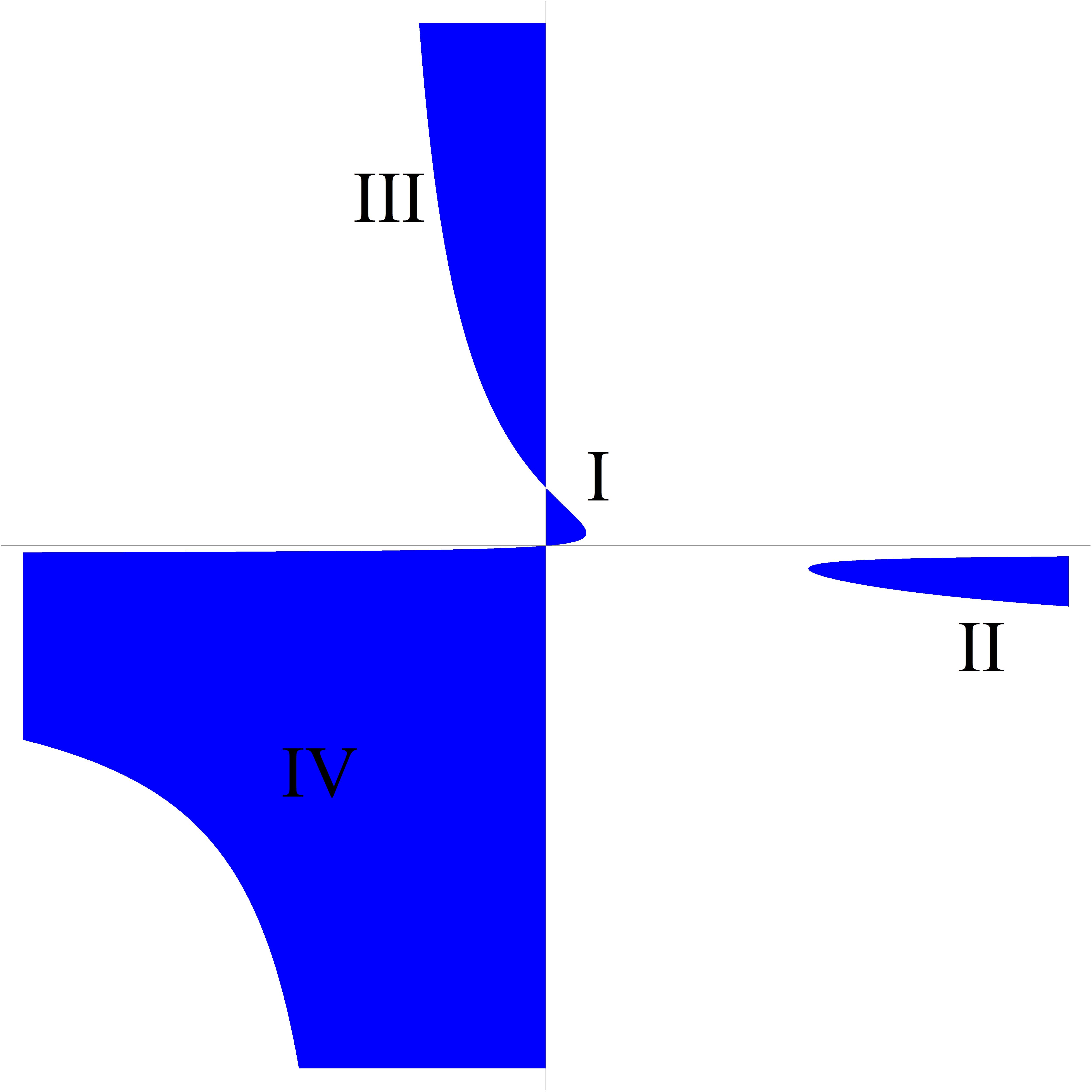
Figure 9: Subregions for the integration of the double box diagram with two adjacent external massive leg on the maximal cut. The parameters for this plot are set as $s=1$, $\chi=1/3$, $\kappa_{1}=1/5$ and $\kappa_{2}=1/7$. On the horizontal and vertical axis we have $x$ and $y$, respectively.

Explicitly, we can check that on the four subregions the conditions $\mu_{11}(z)\geq 0$ and $\mu_{22}(z)\geq 0$ are satisfied.

Again, the integrals under consideration are

$$I[n_{1},n_{2},\ldots,n_{7},-a,-b]\equiv\int\frac{d^{D}l_{1}}{\pi^{D/2}}\frac{d^{D}l_{2}}{\pi^{D/2}}\frac{D_{8}^{a}D_{9}^{b}}{D_{1}^{n_{1}}D_{2}^{n_{2}}\ldots D_{7}^{n_{7}}}\,.$$ (117)

Again we define $J[a,b]\equiv I[1,1,1,1,1,1,1,-a,-b]$. The integration over $\Omega_{\text{I}}$ contains a $y$-integral for $y^{(\ldots)}(\chi-y)^{(\ldots)}(y-c_{1})^{(\ldots)}(y-c_{2})^{(\ldots)}$, hence the result contains the Appell F1 function. Explicitly,

$$J[a,b]\big{|}_{\rm m.c.}^{(\text{I})}=\left(\kappa_{1}\kappa_{2}\right){}^{-a-\frac{D}{2}+2}\left(\left(\kappa_{1}-\chi\right)\left(\kappa_{2}-\chi\right)+\chi\right){}^{2-\frac{D}{2}}s^{a+b+D-7}\chi^{2a+b+2D-9}\,$$

$$\times\frac{\Gamma\left(\frac{D}{2}-2\right)\Gamma\left(a+\frac{D}{2}-2\right)\Gamma(a+b+D-4)}{16\pi^{4}\Gamma(D-4)\Gamma(2a+b+2D-8)}\,$$

$$\times F_{1}\left(a+b+D-4;\frac{1}{2}(2a+D-4),\frac{1}{2}(2a+D-4);2a+b+2D-8;w_{1},w_{2}\right)\,.$$ (118)

where $F_{1}$ is the Appell F1 function. The arguments $w_{1}$ and $w_{2}$ are defined as

$$w_{1}=\frac{\chi}{\kappa_{1}\kappa_{2}}c_{1},\quad w_{2}=\frac{\chi}{\kappa_{1}\kappa_{2}}c_{2}\,.$$ (119)

The integration over $\Omega_{\text{II}}$ reads

$$J[a,b]\big{|}_{\rm m.c.}^{(\text{II})}=4^{a-2}(-1)^{b}\left(w_{1}-w_{2}\right){}^{5}\left(1-w_{2}\right){}^{a+D-5}\left(\frac{w_{1}}{w_{2}}+\frac{w_{2}}{w_{1}}-2\right){}^{-a-\frac{D}{2}}w_{1}^{-3}\left(-w_{2}\right){}^{-2a-b-2D+7}$$

$$\times\left(\left(\kappa_{1}-\chi\right)\left(\kappa_{2}-\chi\right)+\chi\right){}^{2-\frac{D}{2}}(\kappa_{1}\kappa_{2})^{-a-\frac{D}{2}+2}s^{a+b+D-7}\chi^{2a+b+2D-9}\frac{\Gamma(-a-D+5)}{\pi^{3}\Gamma\left(\frac{D-3}{2}\right)\Gamma\left(-a-\frac{D}{2}+\frac{7}{2}\right)}$$

$$\times F_{1}\left(-a-\frac{D}{2}+3;-a-b-D+5,-a-D+5;-2a-D+6;1-\frac{w_{2}}{w_{1}},\frac{w_{1}-w_{2}}{w_{1}-w_{1}w_{2}}\right)\,.$$ (120)

The integration over $\Omega_{\text{III}}$ is

$$J[a,b]\big{|}_{\rm m.c.}^{(\text{III})}=(-1)^{a}\left(\left(\kappa_{1}-\chi\right)\left(\kappa_{2}-\chi\right)+\chi\right){}^{2-\frac{D}{2}}s^{a+b+D-7}\chi^{2a+b+2D-9}\left(\kappa_{1}\kappa_{2}w_{1}w_{2}\right){}^{-a-\frac{D}{2}+2}$$

$$\frac{\Gamma\left(\frac{D}{2}-2\right)\Gamma\left(a+\frac{D}{2}-2\right)\Gamma(-b-D+5)F_{1}\left(-b-D+5;a+\frac{D}{2}-2,a+\frac{D}{2}-2;a-b+1;\frac{1}{w_{1}},\frac{1}{w_{2}}\right)}{16\pi^{4}\Gamma(D-4)\Gamma(a-b+1)}\,.$$ (121)

We can check that the last integration over $\Omega_{\text{IV}}$ is dependent,

$$J[a,b]\big{|}_{\rm m.c.}^{(\text{IV})}=J[a,b]\big{|}_{\rm m.c.}^{(\text{I})}-2\cos(\pi D)J[a,b]\big{|}_{\rm m.c.}^{(\text{III})}\,.$$ (122)

Hence we define the maximal cut as the collection of three cut functions,

$$J[a,b]\big{|}_{\rm m.c.}=\bigg{(}J[a,b]\big{|}_{\rm m.c.}^{(\text{I})},J[a,b]\big{|}_{\rm m.c.}^{(\text{II})},J[a,b]\big{|}_{\rm m.c.}^{(\text{III})}\bigg{)}\,.$$ (123)

There are three master integrals for this diagram on the maximal cut, namely $J[0,0]$, $J[1,0]$ and $J[0,1]$. As was the case for the $\,{}_{2}F_{1}$ function, the contiguous relations of Appell F1 functions generate IBP relations on the maximal cut level. We see that the cut functions on all four subregions, $J[a,b]\big{|}_{\rm m.c.}^{(i)}$, $i=$I, II, III, IV, satisfy IBP relations on the maximal cut. For example,

$$J[1,1]\big{|}_{\rm m.c.}^{(i)}=\frac{1}{2}s^{2}\chi J[0,0]\big{|}_{\rm m.c.}^{(i)}+\frac{1}{2}\left(\kappa_{1}+\kappa_{2}-1\right)sJ[1,0]\big{|}_{\rm m.c.}^{(i)}-sJ[0,1]\big{|}_{\rm m.c.}^{(i)}\,,$$

$$J[2,0]\big{|}_{\rm m.c.}^{(i)}=-\frac{(D-4)\left(\kappa_{1}+\kappa_{2}-1\right)s^{2}\chi}{2(D-3)\left(\kappa_{1}^{2}-2\kappa_{2}\kappa_{1}-2\kappa_{1}+\kappa_{2}^{2}-2\kappa_{2}+1\right)}J[0,0]\big{|}_{\rm m.c.}^{(i)}\,$$

$$-\frac{s}{2(D-3)\left(\kappa_{1}^{2}-2\kappa_{2}\kappa_{1}-2\kappa_{1}+\kappa_{2}^{2}-2\kappa_{2}+1\right)}\bigg{(}2D\kappa_{1}\chi+2D\kappa_{2}\chi+D\kappa_{1}^{2}-2D\kappa_{1}-6D\kappa_{2}\kappa_{1}+$$

$$D\kappa_{2}^{2}-2D\kappa_{2}-2D\chi+D-6\kappa_{1}\chi-6\kappa_{2}\chi-4\kappa_{1}^{2}+20\kappa_{2}\kappa_{1}+8\kappa_{1}-4\kappa_{2}^{2}+8\kappa_{2}+6\chi-4\bigg{)}J[1,0]\big{|}_{\rm m.c.}^{(i)}\,$$

$$+\frac{(D-4)s\left(\kappa_{1}+\kappa_{2}-\chi-1\right)}{(D-3)\left(\kappa_{1}^{2}-2\kappa_{2}\kappa_{1}-2\kappa_{1}+\kappa_{2}^{2}-2\kappa_{2}+1\right)}J[0,1]\big{|}_{\rm m.c.}^{(i)}\,.$$ (124)

Similarly, $J[a,b]\big{|}_{\rm m.c.}^{(i)}$, $i=$I, II, III, IV, satisfy dimension-shift identities because of Appell F1 functions’ contiguous relations.

Let $I=(J[0,0],J[1,0],J[0,1])^{T}$. $I$ should satisfy the differential equations on the maximal cut,

$$\frac{\partial}{\partial\chi}I=M_{\chi}I+\ldots,\quad\frac{\partial}{\partial\kappa_{1}}I=M_{\kappa_{1}}I+\ldots,\quad\frac{\partial}{\partial\kappa_{2}}I=M_{\kappa_{2}}I+\ldots\,,$$ (125)

where the $3\times 3$ matrices are given in figure 10.

Figure 10: Matrices for differential equations on the maximal cut for the double box diagram with two adjacent massive legs.

Explicitly, for any $i=$I, II, III, IV, the vector $(J[0,0]\big{|}_{\rm m.c.}^{(i)},J[1,0]\big{|}_{\rm m.c.}^{(i)},J[0,1]\big{|}_{\rm m.c.}^{(i)})^{T}$ solves the differential equations on the maximal cut. Furthermore, we find that the $3\times 3$ matrix

$$S=\left(\begin{array}[]{c}J[0,0]\big{|}_{\rm m.c.}\\ J[1,0]\big{|}_{\rm m.c.}\\ J[0,1]\big{|}_{\rm m.c.}\end{array}\right)\,,$$ (126)

is the fundamental solution matrix for all these differential equations and the Wronskian is nonzero.

The leading coefficients of $S$ in the limit $D\to 4$ are

$$T=\left(\begin{array}[]{ccc}\frac{1}{2\pi^{4}s^{3}\chi}&0&\frac{1}{4\pi^{4}s^{3}\chi}\\ 0&-\frac{1}{4\pi^{4}\sqrt{\kappa_{1}^{2}-2\kappa_{2}\kappa_{1}-2\kappa_{1}+\kappa_{2}^{2}-2\kappa_{2}+1}s^{2}}&0\\ \frac{1}{4\pi^{4}s^{2}}&0&\frac{1}{4\pi^{4}s^{2}}\\ \end{array}\right)\,.$$ (127)

By a simple column operation, the transformation matrix can be chosen as

$$\tilde{T}=T.\left(\begin{array}[]{ccc}1&0&1\\ 0&1&0\\ -1&0&-2\end{array}\right)4\pi^{4}=\left(\begin{array}[]{ccc}\frac{1}{s^{3}\chi}&0&0\\ 0&-\frac{1}{\sqrt{\kappa_{1}^{2}-2\kappa_{2}\kappa_{1}-2\kappa_{1}+\kappa_{2}^{2}-2\kappa_{2}+1}s^{2}}&0\\ 0&0&-\frac{1}{s^{2}}\\ \end{array}\right)\,.$$ (128)

So we can redefine the basis as

$$\tilde{I}=(s^{3}\chi J[0,0],-s^{2}\sqrt{\kappa_{1}^{2}-2\kappa_{2}\kappa_{1}-2\kappa_{1}+\kappa_{2}^{2}-2\kappa_{2}+1}J[1,0],-s^{2}J[0,1])^{T}\,.$$ (129)

The differential equations on the maximal cut for $\tilde{I}$ is in the $\epsilon$-form,

$$\frac{\partial}{\partial\chi}\tilde{I}=(D-4)\tilde{B}_{\chi}\tilde{I}+\ldots,\quad\frac{\partial}{\partial\kappa_{1}}\tilde{I}=(D-4)\tilde{B}_{\kappa_{1}}\tilde{I}+\ldots,\quad\frac{\partial}{\partial\kappa_{2}}\tilde{I}=(D-4)\tilde{B}_{\kappa_{2}}\tilde{I}+\ldots\,,$$ (130)

where the matrices $\tilde{B}_{\chi}$, $\tilde{B}_{\kappa_{1}}$ and $\tilde{B}_{\kappa_{2}}$ are given in figure 11. Again $\ldots$ stands for integrals with fewer propagators.

Figure 11: Matrices for the $\epsilon$-form differential equations on the maximal cut for the double box diagram with two adjacent massive legs.

6 Nonplanar maximal cuts with two ISPs

We are also interested in confirming that nonplanar integrals are equally amenable to the $D$-dimensional maximal cut procedure demonstrated for one-loop and planar two-loop integrals throughout the previous sections. More specifically, we analyze the maximal cut regions for the purely massless nonplanar double box, evaluate the two-fold integral in the post-hepta-cut degrees of freedom for each subregion separately, and finally investigate the properties of the resulting maximal cut expression.

6.1 Massless nonplanar double box

We adopt the conventions for the external kinematics from the preceeding section. Consider now a generic purely massless $D$-dimensional nonplanar double-box integral,

$$X[n_{1},n_{2},\dots,n_{7},-a,-b]=\int\frac{d^{D}l_{1}}{\pi^{D/2}}\int\frac{d^{D}l_{2}}{\pi^{D/2}}\frac{D_{8}^{a}D_{9}^{b}}{D_{1}^{n_{1}}D_{2}^{n_{2}}\cdots D_{7}^{n_{7}}}\,,$$ (131)

specified by the seven inverse propagators,

$$D_{1}=\ell_{1}^{2}\,,\quad D_{2}=(\ell_{1}-k_{1})^{2}\,,\quad D_{3}=(\ell_{1}-k_{1}-k_{2})^{2}\,,\quad D_{4}=\ell_{2}^{2}\,,$$ (132)

$$D_{5}=(\ell_{2}-k_{4})^{2}\,,\quad D_{6}=(\ell_{1}+\ell_{2})^{2}\,,\quad D_{7}=(\ell_{1}+\ell_{2}+k_{3})^{2}\,,$$ (133)

and two ISPs, which may be picked up as the conventional propagator-like forms,

$$D_{8}=(\ell_{1}+k_{1})^{2}\,,\quad D_{9}=(\ell_{2}+k_{4})^{2}\;.$$ (134)

The momentum flow conventions corresponding to the integral under consideration are shown in figure 12.

Figure 12: The nonplanar double box with four external lines.

The maximal cut evaluated in the Baikov representation reads

$$X[a,b]\big{|}_{\rm m.c.}^{(\Omega)}=\frac{2^{D-5}}{\pi^{4}\Gamma(D-4)\det G_{3}}\int_{\Omega}dz_{8}dz_{9}z_{8}^{a}z_{9}^{b}F(z_{8},z_{9})^{\frac{D-6}{2}}\,,$$ (135)

where

$$F(z_{8},z_{9})=\frac{z_{8}z_{9}\left(s+z_{8}\right)\left(s\chi-z_{8}-z_{9}\right)}{4s^{2}\chi(\chi+1)}\;.$$ (136)

This expression for $F$ parallels eq. (77). The domain of integration $\Omega$ is again defined as the region of the $(z_{8},z_{9})$-plane where the cut Baikov polynomial is nonnegative. As shown in figure 13, for the problem at hand, $\Omega$ is divided into five simple subregions. These subregions take the shape of triangles and rectangles, corresponding to the inequalities:

• $z_{8}>0\,,\;z_{9}>0\,,\;s+z_{8}>0\,,\;t-z_{8}-z_{9}>0\,,$

• $z_{8}>0\,,\;z_{9}<0\,,\;s+z_{8}>0\,,\;t-z_{8}-z_{9}<0\,,$

• $z_{8}<0\,,\;z_{9}<0\,,\;s+z_{8}>0\,,\;t-z_{8}-z_{9}>0\,,$

• $z_{8}<0\,,\;z_{9}>0\,,\;s+z_{8}>0\,,\;t-z_{8}-z_{9}<0\,,$

• $z_{8}<0\,,\;z_{9}>0\,,\;s+z_{8}<0\,,\;t-z_{8}-z_{9}>0\,.$

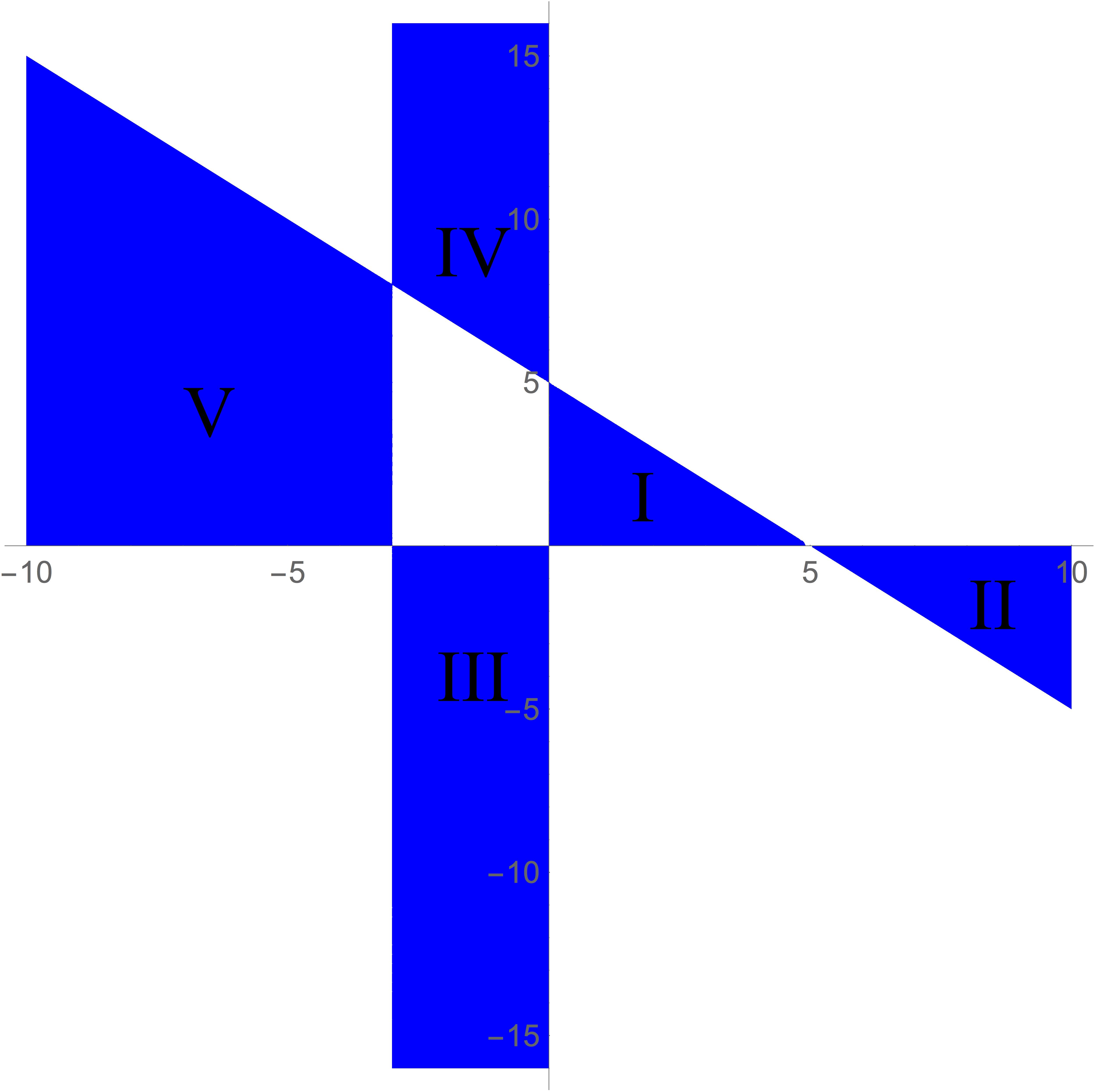
Figure 13: The five regions $\Omega_{I},\dots,\Omega_{V}$ for the maximally cut nonplanar double box with massless internal and external kinematics. The colored area corresponds to $F\geq 0$, where $F$ is the Baikov polynomial. The numeric conditions for this plot are $s=3$ and $t=5$.

We now calculate the double integral for each subregion separately. For example, the integration over region $I$ is parametrized as follows,

$$X[a,b]\big{|}_{\rm m.c.}^{(I)}={} \frac{2^{D-5}}{\pi^{4}\Gamma(D-4)\det G_{3}}\int_{0}^{t}dz_{8}\int_{0}^{t-z_{8}}dz_{9}F(z_{8},z_{9})^{\frac{D-6}{2}}z_{8}^{a}z_{9}^{b}\;.$$ (137)

In this instance and also for the remaining four subregions the result is straightforwardly obtained in the form of ${}_{2}F_{1}$ hypergeometric functions multiplied by kinematic invariants and some Gamma functions as expected. The result for region $I$ can be written as

$$X[a,b]\big{|}_{\rm m.c.}^{(I)}={} \frac{2^{D-5}}{\pi^{4}\Gamma(D-4)}s^{a+b+D-7}\chi^{a+b+D-5}(1+\chi)^{2-\frac{D}{2}}\Gamma\Big{(}a+\frac{D}{2}-2\Big{)}\Gamma\Big{(}b+\frac{D}{2}-2\Big{)}$$

$$\qquad\times\Gamma\Big{(}\frac{D}{2}-2\Big{)}\,_{2}\tilde{F}_{1}\Big{(}3-\frac{D}{2},a+\frac{D}{2}-2;a+b+\frac{3D}{2}-6;-\chi\Big{)}\,.$$ (138)

Completely analogously, for region $II$,

$$X[a,b]\big{|}_{\rm m.c.}^{(II)}={} \frac{2^{D-5}}{\pi^{4}\Gamma(D-4)}(-1)^{b+D}s^{a+b+D-7}\chi^{a+b+\frac{3D}{2}-8}(1+\chi)^{2-\frac{D}{2}}\Gamma(10-a-b-2D)$$

$$\;\;\times\Gamma\Big{(}\frac{D}{2}-2\Big{)}\Gamma\Big{(}b+\frac{D}{2}-2\Big{)}\,_{2}\tilde{F}_{1}\Big{(}10-a-b-2D,3-\frac{D}{2};6-a-D;-\frac{1}{\chi}\Big{)}\,.$$ (139)

Next, we present the results for regions $III$ and $IV$,

$$X[a,b]\big{|}_{\rm m.c.}^{(III)}=\frac{2^{5-D}}{\pi^{4}\Gamma(D-4)}(-1)^{1+a+b}s^{a+b+D-7}\chi^{b+\frac{D}{2}-3}(1+\chi)^{2-\frac{D}{2}}\Gamma(5-b-D)$$ (140)

$$\quad\times\frac{\Gamma\Big{(}a+\frac{D}{2}-2\Big{)}\Gamma\Big{(}b+\frac{D}{2}-2\Big{)}\Gamma\Big{(}\frac{D}{2}-2\Big{)}}{\Gamma\Big{(}3-\frac{D}{2}\Big{)}}\,_{2}\tilde{F}_{1}\Big{(}5-b-D,a+\frac{D}{2}-2;a+D-4;-\frac{1}{\chi}\Big{)}\,,$$

$$X[a,b]\big{|}_{\rm m.c.}^{(IV)}=\frac{2^{D-5}}{\pi^{4}\Gamma(D-4)}(-1)^{a+1}s^{a+b+D-7}\chi^{b+\frac{D}{2}-3}(1+\chi)^{2-\frac{D}{2}}\Gamma(5-b-D)$$

$$\qquad\quad\times\frac{\Gamma\Big{(}a+\frac{D}{2}-2\Big{)}\Gamma^{2}\Big{(}\frac{D}{2}-2\Big{)}}{\Gamma\Big{(}3-b-\frac{D}{2}\Big{)}}\,_{2}\tilde{F}_{1}\Big{(}5-b-D,a+\frac{D}{2}-2;a+D-4;-\frac{1}{\chi}\Big{)}\,.$$ (141)

Finally, the integration over region $V$ yields a slightly more complicated expression involving multiple hypergeometric functions. As we shall see below, the fully simplified output from Mathematica can be further manually reduced to a very compact form.

By inspection of eqs. (138)-(6.1) along with the expression obtained for region $V$, we see that the maximal cut of the nonplanar double box basically gives rise to Gauss’ ${}_{2}F_{1}$ hypergeometric functions with four distinct quadruples of indices, namely,

$${}_{2}\tilde{F}_{1}\Big{(}3-\frac{D}{2},a+\frac{D}{2}-2;a+b+\frac{3D}{2}-6;-\chi\Big{)}\,,$$ (142)

$${}_{2}\tilde{F}_{1}\Big{(}10-a-b-2D,3-\frac{D}{2};6-a-D;-\frac{1}{\chi}\Big{)}\,,$$ (143)

$${}_{2}\tilde{F}_{1}\Big{(}5-b-D,a+\frac{D}{2}-2;a+D-4;-\frac{1}{\chi}\Big{)}\,,$$ (144)

$${}_{2}\tilde{F}_{1}\Big{(}10-a-b-2D,5-b-D;8-a-b-\frac{3D}{2};-\chi\Big{)}\;.$$ (145)

Again, it is however trivial to reexpress two of the hypergeometric functions in terms of the remaining two. For instance, we can choose the integration over regions $I$ and $II$ as the principal results, and simply define the maximal cut function as

$$X[a,b]\big{|}_{\rm m.c.}\equiv\Big{(}X[a,b]\big{|}_{\rm m.c.}^{(I)},X[a,b]\big{|}_{\rm m.c.}^{(II)}\Big{)}\;.$$ (146)

Given that $a$ and $b$ always assume integer values we found the following remarkable simplifications for regions $III$, $IV$ and $V$,

$$X[a,b]\big{|}_{\rm m.c.}^{(III)}={} e^{i\pi D}X[a,b]\big{|}_{\rm m.c.}^{(I)}+2\cos\pi DX[a,b]\big{|}_{\rm m.c.}^{(II)}=X[a,b]\big{|}_{\rm m.c.}^{(IV)}\,,$$ (147)

$$X[a,b]\big{|}_{\rm m.c.}^{(V)}={} e^{i\pi D}X[a,b]\big{|}_{\rm m.c.}^{(I)}+(1+2\cos\pi D)X[a,b]\big{|}_{\rm m.c.}^{(II)}\;.$$ (148)

It is readily verified that all the displayed coefficients can be regarded as merely constants in connection with integral relations, as they are independent of $a$ and $b$, and invariant under dimensional shifts $D\to D\pm 2$.

As for the planar double box, Gauss’ contiguous relations immediately provide all necessary information about the IBPs on the maximal cut by the same argument. From the simple structure of the maximal cut we know that $X[a,b]\big{|}_{\rm m.c.}^{(i)}$ can be reduced to a linear combination of, say, $X[0,0]\big{|}_{\rm m.c.}^{(i)}$ and $X[1,0]\big{|}_{\rm m.c.}^{(i)}$, corresponding to the usual scalar and rank-1 tensor master integrals. This observation holds for any of the five subregions individually. For example, up to rank-2 tensors, for $i=I,II,III,IV,V$,

$$X[0,1]\big{|}_{\rm m.c.}^{(i)}={} +\frac{t}{2}X[0,0]\big{|}_{\rm m.c.}^{(i)}-\frac{1}{2}X[1,0]\big{|}_{\rm m.c.}^{(i)}\,,$$ (149)

$$X[1,1]\big{|}_{\rm m.c.}^{(i)}={} -\frac{1}{8}s\chi X[0,0]\big{|}_{\rm m.c.}^{(i)}+\frac{1}{8}s(2\chi+3)X[1,0]\big{|}_{\rm m.c.}^{(i)}\,,$$ (150)

$$X[2,0]\big{|}_{\rm m.c.}^{(i)}={} +\frac{1}{4}s^{2}\chi X[0,0]\big{|}_{\rm m.c.}^{(i)}-\frac{1}{4}s(3-2\chi)X[1,0]\big{|}_{\rm m.c.}^{(i)}\,,$$ (151)

$$X[0,2]\big{|}_{\rm m.c.}^{(i)}={} +\frac{(D-2)s^{2}\chi(4\chi+1)}{16(D-3)}X[0,0]\big{|}_{\rm m.c.}^{(i)}-\frac{3(D-2)s(2\chi+1)}{16(D-3)}X[1,0]\big{|}_{\rm m.c.}^{(i)}\;.$$ (152)

An elementary manipulation of eq. (146) enables us to also include nonplanar double box integrals with doubled (or simply arbitrary powers of) propagators in the present setup. Here, however, we refrain for brevity from giving any examples along this direction. Instead, we verify that our maximal cut inherits the dimension shifting properties satisfied by the uncut integral. Explicitly, it can be shown that the maximal cut satisfies the raising recurrence relation,

$$X[0,0]\big{|}_{\rm m.c.}^{(i)}(D-2)=$$

$$\frac{D-5}{(D-6)s^{2}\chi^{2}(\chi+1)^{2}}\Big{(}2(3D-16)(10D-47)\chi+3(9(D-10)D+224)$$

$$\qquad\qquad-16(D-5)^{2}\chi^{4}-8(D-5)(2D-11)\chi^{3}+24(D-5)^{2}\chi^{2}\Big{)}X[0,0]\big{|}_{\rm m.c.}^{(i)}(D)$$

$$\quad+\frac{2(D-5)(2D-9)(2\chi+1)(D(4\chi(\chi+1)+9)-4(5\chi(\chi+1)+12))}{(D-6)s^{3}\chi^{2}(\chi+1)^{2}}X[1,0]\big{|}_{\rm m.c.}^{(i)}(D)\,,$$ (153)

and also the lowering recurrence relation,

$$X[0,0]\big{|}_{\rm m.c.}^{(i)}(D+2)=$$

$$\quad\frac{(D-4)s^{2}(D(4(\chi-2)\chi-3)+4\chi(7-3\chi)+10)}{128(D-3)^{3}(2D-7)(\chi+1)}X[0,0]\big{|}_{\rm m.c.}^{(i)}(D)$$

$$\qquad+\frac{(D-4)s(2\chi+1)(D(4\chi(\chi+1)+9)-6(2\chi(\chi+1)+5))}{128(D-3)^{3}(2D-7)\chi(\chi+1)}X[1,0]\big{|}_{\rm m.c.}^{(i)}(D)\;.$$ (154)

These equations are true for any of the five subregions. Similar identities hold for all other nonplanar double box integrals. All integral relations inferred from the maximal cut are validated by FIRE Smirnov:2005ky ; Smirnov:2006tz ; Smirnov:2008iw ; Smirnov:2014hma and Azurite Georgoudis:2016wff .

Let us finally discuss differential equations obeyed by the nonplanar double box integrals and their relation to the maximal cut. From the IBP relations it has already been established that

$$\frac{d}{d\chi}\left(\begin{array}[]{c}\tilde{J}[0,0]\\ \tilde{J}[1,0]\end{array}\right)=\left(\begin{array}[]{cc}\frac{D-\chi-5}{\chi(\chi+1)}&\frac{2D-9}{s\chi(\chi+1)}\\ \frac{(D-4)s}{2(\chi+1)}&\frac{2\chi D-D-10\chi+4}{2\chi(\chi+1)}\\ \end{array}\right)\left(\begin{array}[]{c}\tilde{J}[0,0]\\ \tilde{J}[1,0]\end{array}\right)+\cdots\,,$$ (155)

suppressing integrals with fewer than seven propagators. We have explicitly checked that our maximal cut indeed solves this differential equation, region by region. Moreover, the maximal cut functions (146) again form the Wronskian matrix $S$ associated with this system of differential equations. Defining $S$ as follows,

$$S=\left(\begin{array}[]{c}X[0,0]\big{|}_{\rm m.c.}\\[2.84526pt] X[1,0]\big{|}_{\rm m.c.}\end{array}\right)\,,$$

the Wronskian determinant is found to be nonvanishing,

$$\det S\propto\chi^{\frac{D}{2}-3}(\chi+1)^{\frac{D}{2}-3}\;.$$ (156)

This ensures that $X[a,b]\big{|}_{\rm m.c.}^{(I)}$ and $X[a,b]\big{|}_{\rm m.c.}^{(II)}$ are linearly independent functions of $\chi$ as previously anticipated, and furthermore confirms that the columns of $S$ form the two fundamental solutions to eq. (155). The leading terms of $S$ in the limit $D\to 4$,

$$T=\frac{16}{\pi^{4}}\left(\begin{array}[]{cc}\frac{2\chi+3}{s^{3}\chi(\chi+1)}&-\frac{1}{s^{3}\chi(\chi+1)}\\ \frac{1}{s^{2}(\chi+1)}&-\frac{1}{s^{2}(\chi+1)}\\ \end{array}\right)$$ (159)

again help us to identify a new set of master integrals in order to transform eq. (155) to $\epsilon$-form. We may include a trivial redefinition of $T$ and take the transformation matrix as

$$T^{\prime}=T\left(\begin{array}[]{cc}1&-4\\ 0&-4\\ \end{array}\right)\cdot\frac{\pi^{4}}{16}\,,$$ (162)

which by eq. (12) implies that

$$\frac{d}{d\chi}\left(\begin{array}[]{c}\tilde{J}_{1}\\ \tilde{J}_{2}\end{array}\right)=(D-4)\left(\begin{array}[]{cc}\frac{2\chi+1}{\chi(\chi+1)}&-\frac{4}{\chi}\\ \frac{1}{2(\chi+1)}&-\frac{2\chi+1}{2\chi(\chi+1)}\\ \end{array}\right)\left(\begin{array}[]{c}\tilde{J}_{1}\\ \tilde{J}_{2}\end{array}\right)\,,$$ (169)

where the modified masters $\tilde{J}_{1}$ and $\tilde{J}_{2}$ denote the following mixture of the FIRE basis integrals,

$$\tilde{J}_{1}\equiv s^{2}(1+\chi)J[1,0]\,,\quad\tilde{J}_{2}\equiv-\frac{1}{8}s^{3}\chi J[0,0]+\frac{1}{8}s^{2}(2\chi+3)J[1,0]=sJ[1,1]\;.$$ (170)

The new differential equation is obviously in $\epsilon$-form for $D=4-2\epsilon$.

In summary, we have explicitly verified that all salient features of the maximal cut of the planar double box carry over immediately to the nonplanar double box. Our example here only covered the purely massless case, but we also have succesfully checked several configurations with massive external momenta.

7 Conclusion

In this paper we have presented a precise and consistent technique for evaluating generalized cuts of multiloop Feynman integrals, properly regularized in $D$ dimensions. Our method relies on the Baikov representation, which makes the effect of taking these generalized cuts in arbitrary dimension manifest. We have given examples of the method for several integral topologies with various kinematic configurations, including the one-loop box, two-loop sunset, planar double box and nonplanar double box.

The simplest instance is the maximal cut of a $k$-propagator integral realized by the multivariate residue of the integrand at $z_{1}=\cdots=z_{k}=0$, the $z_{i}$’s being the Baikov variables. In general the maximal cut leaves a multi-fold integral over a domain $\Omega$ defined by the intersection of the cut hyperplanes and the region $A$ where the Baikov kernel $F$ is nonnegative. The remaining integration may be carried out over any subregion of $\Omega$ with $F=0$ on the boundary. We refer to the result as the maximal cut function on subregion $j$; this can be viewed as a generalization of the notion of a composite leading singularity.

The maximal cut function satisfies the same form of integral relations, such as IBPs and dimension shift identities, and differential equations as the uncut integral, region by region. In our examples, the maximal cut functions are compact analytic expressions involving Gamma functions and (generalized-) hypergeometric functions. The integral identities on the maximal cut hence immediately correspond to relations among these special functions, namely recurrence relations and Gauss’ contiguous relations.

One of the principal features of all our examples is that an integral topology with $m$ master integrals has precisely $m$ linearly independent maximal cut function series. For instance, the purely nonplanar double box, with real kinematics, gives rise to five subregions, but only two linearly independent maximal cut functions. This number agrees with the number of master integrals. We have explicitly shown that the linearly independent maximal cut functions form the Wronskian matrix $S$ for the system of differential equations on the maximal cut. Moreover, we have in detail demonstrated that the leading terms of $S$ provide a transformation matrix for differential equation into to canonical (epsilon) form near four dimensions.

From the viewpoint of the differential equation of Feynman integrals without cut, these maximal-cut functions form the fundamental solution set of the “homogenous” equation. To solve the complete differential equation system, can be understood as solving for an “inhomogenous” differential equation. Hence it is expected that these functions would appear in the complete expression of Feynman integrals.

This work brings inspiration for further advances along the direction of multiloop generalized unitarity with arbitrary spacetime dimension.

• In this paper, we simply consider the integration regions corresponding to the real loop momenta and find that it is enough to get the complete solutions for the differential equations on the maximal cut. For more complicated integrals, we may also consider complex loop momenta and integration regions for complex Baikov variables. (For a region to be valid, we still require that on the boundary the Baikov polynomial vanishes, i.e., $F=0$.)

• It would be very interesting to study the maximal cut of elliptic Feynman integrals Laporta:2004rb ; Bloch:2013tra ; Adams:2013kgc ; Adams:2014vja ; Adams:2015gva ; Bloch:2016izu ; Passarino:2016zcd ; Kalmykov:2016lxx ; vonManteuffel:2017hms ; Adams:2017tga with arbitrary spacetime dimension. The $4D$ maximal cut of an elliptic double box was studied via Weierstrass elliptic functions Sogaard:2014jla . The $(D-2)$-iterative form of elliptic differential equations were studied in ref. Adams:2015ydq ; Tancredi:2015bvi ; Remiddi:2016gno . We expect that our method combined with integrals over the fundamental domain of elliptic curves, would provide the maximal cut of elliptic Feynman integrals in a closed form of $D$.

• It is also interesting to see the non-maximal cut in $D$-dimension. We may either directly carry out Baikov integrals with non-maximal cut, or extend known maximal-cut functions to the non-maximal cut results via the block-triangular differential equation.

Appendix A Rudiments of hypergeometric identities

In this appendix, we list several identities for hypergeometric functions which are used in this paper. The discussion follows MR1424469 ; MR1034956 .

Hypergeometric $\,{}_{2}F_{1}$ functions are the solutions of Fuchsian equations with three regular singular points on $\mathbb{CP}^{1}$. With Taylor series, it is defined as

$$\,_{2}F_{1}(\alpha,\beta,\gamma,z)=\sum_{n=0}^{\infty}\frac{(\alpha)_{n}(\beta)_{n}}{n!(\gamma)_{n}}z^{n},\quad|z|<1\,,$$ (171)

where the Pochhammer symbol (26) is used. For other points (except $z=1$) on the complex plane, $\,{}_{2}F_{1}(z)$ can be defined by analytic continuation.

$\,{}_{2}F_{1}(z)$ satisfies the Fuchsian equation (when $\gamma\not\in\mathbb{Z}_{\leq 0}$),

$$z(1-z)\frac{d^{2}f}{dz^{2}}+\big{(}\gamma-(\alpha+\beta+1)z\big{)}\frac{df}{dz}-\alpha\beta f=0\,.$$ (172)

The other independent solution is (when $\gamma\not\in\mathbb{Z}$),

$$z^{1-\gamma}\,_{2}F_{1}(\alpha-\gamma+1,\beta-\gamma+1,2-\gamma,z)\,.$$ (173)

It is possible to study the solution of (172) near the other singular two points $1$ and $\infty$, and the solution will be hypergeometric functions with the fourth arguments $1-z$ and $1/z$. By the linear dependence of solutions, there are relations,

$$\,{}_{2}F_{1}(\alpha,\beta,\gamma,z) =\frac{\Gamma(\gamma)\Gamma(\alpha+\beta-\gamma)(1-z)^{-\alpha-\beta+\gamma}\,_{2}F_{1}(\gamma-\alpha,\gamma-\beta;-\alpha-\beta+\gamma+1;1-z)}{\Gamma(\alpha)\Gamma(\beta)}$$

$$+\frac{\Gamma(\gamma)\Gamma(-\alpha-\beta+\gamma)\,_{2}F_{1}(\alpha,\beta;\alpha+\beta-\gamma+1;1-z)}{\Gamma(\gamma-\alpha)\Gamma(\gamma-\beta)}\,,$$ (174)

$$\,{}_{2}F_{1}(\alpha,\beta,\gamma,z) =\frac{\Gamma(\gamma)(-z)^{-\alpha}\Gamma(\beta-\alpha)\,_{2}F_{1}\left(\alpha,\alpha-\gamma+1;\alpha-\beta+1;\frac{1}{z}\right)}{\Gamma(\beta)\Gamma(\gamma-\alpha)}$$

$$+\frac{\Gamma(\gamma)(-z)^{-\beta}\Gamma(\alpha-\beta)\,_{2}F_{1}\left(\beta,\beta-\gamma+1;-\alpha+\beta+1;\frac{1}{z}\right)}{\Gamma(\alpha)\Gamma(\gamma-\beta)}\,.$$ (175)

Euler’s transformation of hypergeometric $\,{}_{2}F_{1}$ functions is

$$\,{}_{2}F_{1}(\alpha,\beta_{,}\gamma_{,}z)=(1-z)^{\gamma-\alpha-\beta}\,_{2}F_{1}(\gamma-\alpha,\gamma-\beta_{,}\gamma_{,}z)\,.$$ (176)

When calculating the maximal cut functions of different subregions, we frequently use (174), (175) and (176) to connect various $\,{}_{2}F_{1}$ functions.

The functions $\,{}_{2}F_{1}(\alpha+l,\beta+m,\gamma+n,z)$, with $l,m,n\in\mathbb{Z}$ are called “contiguous” to the function $\,{}_{2}F_{1}(\alpha,\beta,\gamma,z)$. Any three contiguous $\,{}_{2}F_{1}$ functions satisfy Gauss’ contiguous relations,

$$A_{1}F_{1}+A_{2}F_{2}+A_{3}F_{3}=0\,,$$ (177)

where the coefficients $A_{i}$’s are rational functions in $\alpha$, $\beta$, $\gamma$ and $z$. The two fundamental Gauss’ contiguous relations follow from the integral representation of $\,{}_{2}F_{1}(z)$,

$$(\gamma-1)\,_{2}F_{1}(\alpha,\beta,\gamma-1,z)-\alpha\,_{2}F_{1}(\alpha+1,\beta_{,}\gamma_{,}z)-(\gamma-\alpha-1)\,_{2}F_{1}(\alpha,\beta_{,}\gamma_{,}z)=0\,$$ (178)

$$\gamma\,_{2}F_{1}(\alpha,\beta,\gamma,z)-\beta z\,_{2}F_{1}(\alpha,\beta+1,\gamma+1,z)-\gamma\,_{2}F_{1}(\alpha-1,\beta,\gamma,z)=0\,,$$ (179)

and all other Gauss’ contiguous relations can be derived from these two. We use these relations for studying the IBPs and dimension-shift identities on the maximal cut level.

When studying the maximal cut in arbitrary dimension, we also meet generalized hypergeometric functions, for example, the Appell F1 function. It has four parameters and two variables, and is defined as,

$$F_{1}(\alpha;\beta_{1},\beta_{2};\gamma;x,y)=\sum_{m=0}^{\infty}\sum_{n=0}^{\infty}\frac{(\alpha)_{m+n}(\beta_{1})_{m}(\beta_{2})_{n}}{m!n!(\gamma)_{m+n}}x^{m}y^{n},\quad|x|<1,|y|<1.$$ (180)

It can be defined outside the polydisc by analytic continuation.

One-variable integrals with four distinct factors can be expressed as the Appell F1 function, for instance,

$$\int_{0}^{1}u^{\alpha-1}(1-u)^{\gamma-\alpha-1}(1-ux)^{-\beta_{1}}(1-uy)^{-\beta_{2}}du=\frac{\Gamma(\alpha)\Gamma(\gamma-\alpha)}{\Gamma(\gamma)}F_{1}(\alpha;\beta_{1},\beta_{2};\gamma;x,y)\,.$$ (181)

The contiguous relations for Appell F1 functions can be found, for example, in the survey article Schlosser2013 .

References

- (1) Z. Bern, L. J. Dixon, D. C. Dunbar, D. A. Kosower, One loop n point gauge theory amplitudes, unitarity and collinear limits, Nucl.Phys. B425 (1994) 217–260. arXiv:hep-ph/9403226, doi:10.1016/0550-3213(94)90179-1.
- (2) Z. Bern, L. J. Dixon, D. C. Dunbar, D. A. Kosower, Fusing gauge theory tree amplitudes into loop amplitudes, Nucl.Phys. B435 (1995) 59–101. arXiv:hep-ph/9409265, doi:10.1016/0550-3213(94)00488-Z.
- (3) R. Britto, F. Cachazo, B. Feng, Generalized unitarity and one-loop amplitudes in N=4 super-Yang-Mills, Nucl.Phys. B725 (2005) 275–305. arXiv:hep-th/0412103, doi:10.1016/j.nuclphysb.2005.07.014.
- (4) D. Forde, Direct extraction of one-loop integral coefficients, Phys.Rev. D75 (2007) 125019. arXiv:0704.1835, doi:10.1103/PhysRevD.75.125019.
- (5) G. Ossola, C. G. Papadopoulos, R. Pittau, Reducing full one-loop amplitudes to scalar integrals at the integrand level, Nucl.Phys. B763 (2007) 147–169. arXiv:hep-ph/0609007, doi:10.1016/j.nuclphysb.2006.11.012.
- (6) G. Ossola, C. G. Papadopoulos, R. Pittau, On the Rational Terms of the one-loop amplitudes, JHEP 05 (2008) 004. arXiv:0802.1876, doi:10.1088/1126-6708/2008/05/004.
-
(7)
Y. Zhang,
Lecture
Notes on Multi-loop Integral Reduction and Applied Algebraic Geometry,
2016.
arXiv:1612.02249.
URL http://inspirehep.net/record/1502112/files/arXiv:1612.02249.pdf - (8) P. Mastrolia, G. Ossola, On the Integrand-Reduction Method for Two-Loop Scattering Amplitudes, JHEP 1111 (2011) 014. arXiv:1107.6041, doi:10.1007/JHEP11(2011)014.
- (9) S. Badger, H. Frellesvig, Y. Zhang, Hepta-Cuts of Two-Loop Scattering Amplitudes, JHEP 1204 (2012) 055. arXiv:1202.2019, doi:10.1007/JHEP04(2012)055.
- (10) P. Mastrolia, E. Mirabella, G. Ossola, T. Peraro, Integrand-Reduction for Two-Loop Scattering Amplitudes through Multivariate Polynomial Division, Phys.Rev. D87 (2013) 085026. arXiv:1209.4319, doi:10.1103/PhysRevD.87.085026.
- (11) S. Badger, H. Frellesvig, Y. Zhang, A Two-Loop Five-Gluon Helicity Amplitude in QCD, JHEP 12 (2013) 045. arXiv:1310.1051, doi:10.1007/JHEP12(2013)045.
- (12) S. Badger, G. Mogull, A. Ochirov, D. O’Connell, A Complete Two-Loop, Five-Gluon Helicity Amplitude in Yang-Mills Theory, JHEP 10 (2015) 064. arXiv:1507.08797, doi:10.1007/JHEP10(2015)064.
- (13) S. Badger, G. Mogull, T. Peraro, Local integrands for two-loop all-plus Yang-Mills amplitudes, JHEP 08 (2016) 063. arXiv:1606.02244, doi:10.1007/JHEP08(2016)063.
- (14) P. Mastrolia, T. Peraro, A. Primo, Adaptive Integrand Decomposition in parallel and orthogonal space, JHEP 08 (2016) 164. arXiv:1605.03157, doi:10.1007/JHEP08(2016)164.
- (15) S. Badger, C. Brønnum-Hansen, F. Buciuni, D. O’Connell, A unitarity compatible approach to one-loop amplitudes with massive fermionsarXiv:1703.05734.
- (16) D. A. Kosower, K. J. Larsen, Maximal Unitarity at Two Loops, Phys. Rev. D85 (2012) 045017. arXiv:1108.1180, doi:10.1103/PhysRevD.85.045017.
- (17) H. Johansson, D. A. Kosower, K. J. Larsen, Two-Loop Maximal Unitarity with External Masses, Phys.Rev. D87 (2013) 025030. arXiv:1208.1754, doi:10.1103/PhysRevD.87.025030.
- (18) H. Johansson, D. A. Kosower, K. J. Larsen, Maximal Unitarity for the Four-Mass Double BoxarXiv:1308.4632.
- (19) M. Sogaard, Global Residues and Two-Loop Hepta-CutsarXiv:1306.1496.
- (20) M. Sogaard, Y. Zhang, Multivariate Residues and Maximal Unitarity, JHEP 12 (2013) 008. arXiv:1310.6006, doi:10.1007/JHEP12(2013)008.
- (21) M. Sogaard, Y. Zhang, Unitarity Cuts of Integrals with Doubled Propagators, JHEP 07 (2014) 112. arXiv:1403.2463, doi:10.1007/JHEP07(2014)112.
- (22) M. Sogaard, Y. Zhang, Massive Nonplanar Two-Loop Maximal Unitarity, JHEP 12 (2014) 006. arXiv:1406.5044, doi:10.1007/JHEP12(2014)006.
- (23) M. Sogaard, Y. Zhang, Elliptic Functions and Maximal Unitarity, Phys. Rev. D91 (8) (2015) 081701. arXiv:1412.5577, doi:10.1103/PhysRevD.91.081701.
- (24) H. Johansson, D. A. Kosower, K. J. Larsen, M. Søgaard, Cross-Order Integral Relations from Maximal Cuts, Phys. Rev. D92 (2) (2015) 025015. arXiv:1503.06711, doi:10.1103/PhysRevD.92.025015.
- (25) S. Abreu, F. Febres Cordero, H. Ita, M. Jaquier, B. Page, Subleading Poles in the Numerical Unitarity Method at Two LoopsarXiv:1703.05255.
- (26) S. Abreu, F. Febres Cordero, H. Ita, M. Jaquier, B. Page, M. Zeng, Two-Loop Four-Gluon Amplitudes with the Numerical Unitarity MethodarXiv:1703.05273.
- (27) J. Gluza, K. Kajda, D. A. Kosower, Towards a Basis for Planar Two-Loop Integrals, Phys.Rev. D83 (2011) 045012. arXiv:1009.0472, doi:10.1103/PhysRevD.83.045012.
- (28) A. V. Kotikov, Differential equation method: The Calculation of N point Feynman diagrams, Phys. Lett. B267 (1991) 123–127, [Erratum: Phys. Lett.B295,409(1992)]. doi:10.1016/0370-2693(91)90536-Y,10.1016/0370-2693(92)91582-T.
- (29) A. V. Kotikov, Differential equations method: New technique for massive Feynman diagrams calculation, Phys. Lett. B254 (1991) 158–164. doi:10.1016/0370-2693(91)90413-K.
- (30) Z. Bern, L. J. Dixon, D. A. Kosower, Dimensionally regulated one loop integrals, Phys. Lett. B302 (1993) 299–308, [Erratum: Phys. Lett.B318,649(1993)]. arXiv:hep-ph/9212308, doi:10.1016/0370-2693(93)90469-X,10.1016/0370-2693(93)90400-C.
- (31) E. Remiddi, Differential equations for Feynman graph amplitudes, Nuovo Cim. A110 (1997) 1435–1452. arXiv:hep-th/9711188.
- (32) T. Gehrmann, E. Remiddi, Differential equations for two loop four point functions, Nucl.Phys. B580 (2000) 485–518. arXiv:hep-ph/9912329, doi:10.1016/S0550-3213(00)00223-6.
- (33) J. Ablinger, A. Behring, J. Blümlein, A. De Freitas, A. von Manteuffel, C. Schneider, Calculating Three Loop Ladder and V-Topologies for Massive Operator Matrix Elements by Computer Algebra, Comput. Phys. Commun. 202 (2016) 33–112. arXiv:1509.08324, doi:10.1016/j.cpc.2016.01.002.
- (34) K. Chetyrkin, F. Tkachov, Integration by Parts: The Algorithm to Calculate beta Functions in 4 Loops, Nucl.Phys. B192 (1981) 159–204. doi:10.1016/0550-3213(81)90199-1.
- (35) J. M. Henn, Multiloop integrals in dimensional regularization made simple, Phys. Rev. Lett. 110 (2013) 251601. arXiv:1304.1806, doi:10.1103/PhysRevLett.110.251601.
- (36) J. M. Henn, Lectures on differential equations for Feynman integrals, J. Phys. A48 (2015) 153001. arXiv:1412.2296, doi:10.1088/1751-8113/48/15/153001.
- (37) R. N. Lee, Reducing differential equations for multiloop master integrals, JHEP 04 (2015) 108. arXiv:1411.0911, doi:10.1007/JHEP04(2015)108.
- (38) M. Argeri, S. Di Vita, P. Mastrolia, E. Mirabella, J. Schlenk, U. Schubert, L. Tancredi, Magnus and Dyson Series for Master Integrals, JHEP 03 (2014) 082. arXiv:1401.2979, doi:10.1007/JHEP03(2014)082.
- (39) C. Meyer, Transforming differential equations of multi-loop Feynman integrals into canonical formarXiv:1611.01087.
- (40) M. Prausa, epsilon: A tool to find a canonical basis of master integralsarXiv:1701.00725.
- (41) O. Gituliar, V. Magerya, Fuchsia: a tool for reducing differential equations for Feynman master integrals to epsilon formarXiv:1701.04269.
- (42) L. Adams, E. Chaubey, S. Weinzierl, Simplifying differential equations for multi-scale Feynman integrals beyond multiple polylogarithms, Phys. Rev. Lett. 118 (14) (2017) 141602. arXiv:1702.04279, doi:10.1103/PhysRevLett.118.141602.
- (43) H. Frellesvig, C. G. Papadopoulos, Cuts of Feynman Integrals in Baikov representationarXiv:1701.07356.
- (44) P. A. Baikov, Explicit solutions of n loop vacuum integral recurrence relationsarXiv:hep-ph/9604254.
- (45) P. A. Baikov, Explicit solutions of the three loop vacuum integral recurrence relations, Phys. Lett. B385 (1996) 404–410. arXiv:hep-ph/9603267, doi:10.1016/0370-2693(96)00835-0.
- (46) P. A. Baikov, A Practical criterion of irreducibility of multi-loop Feynman integrals, Phys. Lett. B634 (2006) 325–329. arXiv:hep-ph/0507053, doi:10.1016/j.physletb.2006.01.052.
- (47) S. Abreu, R. Britto, C. Duhr, E. Gardi, Cuts from residues: the one-loop casearXiv:1702.03163.
- (48) S. Abreu, R. Britto, C. Duhr, E. Gardi, The algebraic structure of cut Feynman integrals and the diagrammatic coactionarXiv:1703.05064.
- (49) A. Primo, L. Tancredi, On the maximal cut of Feynman integrals and the solution of their differential equations, Nucl. Phys. B916 (2017) 94–116. arXiv:1610.08397, doi:10.1016/j.nuclphysb.2016.12.021.
- (50) M. Zeng, Differential equations on unitarity cut surfacesarXiv:1702.02355.
-
(51)
R. N. Lee,
Modern
techniques of multiloop calculations, in: Proceedings, 49th Rencontres de
Moriond on QCD and High Energy Interactions: La Thuile, Italy, March 22-29,
2014, 2014, pp. 297–300.
arXiv:1405.5616.
URL https://inspirehep.net/record/1297497/files/arXiv:1405.5616.pdf - (52) H. Ita, Two-loop Integrand Decomposition into Master Integrals and Surface Terms, Phys. Rev. D94 (11) (2016) 116015. arXiv:1510.05626, doi:10.1103/PhysRevD.94.116015.
- (53) K. J. Larsen, Y. Zhang, Integration-by-parts reductions from unitarity cuts and algebraic geometry, Phys. Rev. D93 (4) (2016) 041701. arXiv:1511.01071, doi:10.1103/PhysRevD.93.041701.
- (54) R. N. Lee, A. A. Pomeransky, Critical points and number of master integrals, JHEP 11 (2013) 165. arXiv:1308.6676, doi:10.1007/JHEP11(2013)165.
- (55) A. Georgoudis, K. J. Larsen, Y. Zhang, Azurite: An algebraic geometry based package for finding bases of loop integralsarXiv:1612.04252.
- (56) A. Smirnov, V. A. Smirnov, Applying Grobner bases to solve reduction problems for Feynman integrals, JHEP 0601 (2006) 001. arXiv:hep-lat/0509187, doi:10.1088/1126-6708/2006/01/001.
- (57) A. Smirnov, An Algorithm to construct Grobner bases for solving integration by parts relations, JHEP 0604 (2006) 026. arXiv:hep-ph/0602078, doi:10.1088/1126-6708/2006/04/026.
- (58) A. Smirnov, Algorithm FIRE – Feynman Integral REduction, JHEP 0810 (2008) 107. arXiv:0807.3243, doi:10.1088/1126-6708/2008/10/107.
- (59) A. V. Smirnov, FIRE5: a C++ implementation of Feynman Integral REduction, Comput. Phys. Commun. 189 (2015) 182–191. arXiv:1408.2372, doi:10.1016/j.cpc.2014.11.024.
- (60) R. N. Lee, Presenting LiteRed: a tool for the Loop InTEgrals REDuctionarXiv:1212.2685.
- (61) R. N. Lee, LiteRed 1.4: a powerful tool for reduction of multiloop integrals, J. Phys. Conf. Ser. 523 (2014) 012059. arXiv:1310.1145, doi:10.1088/1742-6596/523/1/012059.
- (62) J. A. M. Vermaseren, Axodraw, Comput. Phys. Commun. 83 (1994) 45–58. doi:10.1016/0010-4655(94)90034-5.
- (63) D. Binosi, J. Collins, C. Kaufhold, L. Theussl, JaxoDraw: A Graphical user interface for drawing Feynman diagrams. Version 2.0 release notes, Comput. Phys. Commun. 180 (2009) 1709–1715. arXiv:0811.4113, doi:10.1016/j.cpc.2009.02.020.
- (64) R. N. Lee, V. A. Smirnov, The Dimensional Recurrence and Analyticity Method for Multicomponent Master Integrals: Using Unitarity Cuts to Construct Homogeneous Solutions, JHEP 12 (2012) 104. arXiv:1209.0339, doi:10.1007/JHEP12(2012)104.
- (65) T. Huber, D. Maitre, HypExp: A Mathematica package for expanding hypergeometric functions around integer-valued parameters, Comput. Phys. Commun. 175 (2006) 122–144. arXiv:hep-ph/0507094, doi:10.1016/j.cpc.2006.01.007.
- (66) T. Huber, D. Maitre, HypExp 2, Expanding Hypergeometric Functions about Half-Integer Parameters, Comput. Phys. Commun. 178 (2008) 755–776. arXiv:0708.2443, doi:10.1016/j.cpc.2007.12.008.
- (67) S. Laporta, E. Remiddi, Analytic treatment of the two loop equal mass sunrise graph, Nucl. Phys. B704 (2005) 349–386. arXiv:hep-ph/0406160, doi:10.1016/j.nuclphysb.2004.10.044.
- (68) S. Bloch, P. Vanhove, The elliptic dilogarithm for the sunset graph, J. Number Theor. 148 (2015) 328–364. arXiv:1309.5865, doi:10.1016/j.jnt.2014.09.032.
- (69) L. Adams, C. Bogner, S. Weinzierl, The two-loop sunrise graph with arbitrary masses, J. Math. Phys. 54 (2013) 052303. arXiv:1302.7004, doi:10.1063/1.4804996.
- (70) L. Adams, C. Bogner, S. Weinzierl, The two-loop sunrise graph in two space-time dimensions with arbitrary masses in terms of elliptic dilogarithms, J. Math. Phys. 55 (10) (2014) 102301. arXiv:1405.5640, doi:10.1063/1.4896563.
- (71) L. Adams, C. Bogner, S. Weinzierl, The two-loop sunrise integral around four space-time dimensions and generalisations of the Clausen and Glaisher functions towards the elliptic case, J. Math. Phys. 56 (7) (2015) 072303. arXiv:1504.03255, doi:10.1063/1.4926985.
- (72) S. Bloch, M. Kerr, P. Vanhove, Local mirror symmetry and the sunset Feynman integralarXiv:1601.08181.
- (73) G. Passarino, Elliptic Polylogarithms and Basic Hypergeometric Functions, Eur. Phys. J. C77 (2) (2017) 77. arXiv:1610.06207, doi:10.1140/epjc/s10052-017-4623-1.
- (74) M. Yu. Kalmykov, B. A. Kniehl, Counting the number of master integrals for sunrise-type Feynman diagrams via Mellin-Barnes representationarXiv:1612.06637.
- (75) A. von Manteuffel, L. Tancredi, A non-planar two-loop three-point function beyond multiple polylogarithmsarXiv:1701.05905.
- (76) L. Adams, C. Bogner, S. Weinzierl, The iterated structure of the all-order result for the two-loop sunrise integral, J. Math. Phys. 57 (3) (2016) 032304. arXiv:1512.05630, doi:10.1063/1.4944722.
- (77) L. Tancredi, Simplifying Systems of Differential Equations. The Case of the Sunrise Graph, Acta Phys. Polon. B46 (11) (2015) 2125. doi:10.5506/APhysPolB.46.2125.
- (78) E. Remiddi, L. Tancredi, Differential equations and dispersion relations for Feynman amplitudes. The two-loop massive sunrise and the kite integral, Nucl. Phys. B907 (2016) 400–444. arXiv:1602.01481, doi:10.1016/j.nuclphysb.2016.04.013.
-
(79)
E. T. Whittaker, G. N. Watson,
A course of modern
analysis, Cambridge Mathematical Library, Cambridge University Press,
Cambridge, 1996, an introduction to the general theory of infinite processes
and of analytic functions; with an account of the principal transcendental
functions, Reprint of the fourth (1927) edition.
doi:10.1017/CBO9780511608759.
URL http://dx.doi.org/10.1017/CBO9780511608759 -
(80)
Z. X. Wang, D. R. Guo, Special
functions, World Scientific Publishing Co., Inc., Teaneck, NJ, 1989,
translated from the Chinese by Guo and X. J. Xia.
doi:10.1142/0653.
URL http://dx.doi.org/10.1142/0653 -
(81)
M. J. Schlosser, Multiple
Hypergeometric Series: Appell Series and Beyond, Springer Vienna, Vienna,
2013, pp. 305–324.
doi:10.1007/978-3-7091-1616-6_13.
URL http://dx.doi.org/10.1007/978-3-7091-1616-6_13