Explore Inert Dark Matter Blind Spots with Gravitational Wave Signatures
Abstract
Motivated by the absence of dark matter signals in direct detection experiments (such as the recent LUX and PandaX-II experiments) and the discovery of gravitational waves (GWs) at aLIGO, we discuss the possibility to explore a generic classes of scalar dark matter models using the complementary searches via phase transition GWs and the future lepton collider signatures. We focus on the inert scalar multiplet dark matter models and the mixed inert scalar dark matter models, which could undergo a strong first-order phase transitions during the evolution of the early universe, and might produce detectable phase transition GW signals at future GW experiments, such as eLISA, DECIGO and BBO. We find that the future GW signature, together with circular electron-positron collider, could further explore the model’s blind spot parameter region, at which the dark matter-Higgs coupling is identically zero, thus avoiding the dark matter spin-independent direct detection constraints.
I Introduction
A brand new door has been opened to study the fundamental physics and the particle cosmology by the gravitational waves (GWs) after the discovery of the GWs by Advanced Laser Interferometer Gravitational Wave Observatory (aLIGO) Abbott:2016blz . One active research field is the idea of probing the new physics through phase transition GWs, where a strong first-order phase transition (FOPT) is induced by the new physics models and can produce detectable GW signals from three mechanisms: collisions of expanding bubbles walls, magnetohydrodynamic turbulence of bubbles and sound waves in the hot plasma of the early universe Witten:1984rs ; Hogan:1984hx ; Turner:1990rc ; Kamionkowski:1993fg ; Hindmarsh:2013xza ; Hindmarsh:2015qta ; Kosowsky:2001xp ; Caprini:2009yp . Various new physics models have been studied by the new approach of GW signals in the post aLIGO era Huang:2016odd ; Dev:2016feu ; Jaeckel:2016jlh ; Hashino:2016rvx ; Jinno:2016knw ; Yu:2016tar ; Kobakhidze:2016mch ; Huang:2016cjm ; Artymowski:2016tme ; Soni:2016yes ; Balazs:2016tbi ; Dorsch:2016nrg ; Huang:2017laj ; Chao:2017vrq ; Beniwal:2017eik ; Addazi:2017gpt ; Marzola:2017jzl ; Bian:2017wfv , such as the GW detection of the dark matter (DM) Chao:2017vrq ; Beniwal:2017eik , the hidden sector Dev:2016feu ; Jaeckel:2016jlh ; Soni:2016yes ; Addazi:2017gpt ; Huang:2017laj and the electroweak baryogenesis Huang:2016odd ; Huang:2016cjm ; Artymowski:2016tme ; Dorsch:2016nrg ; Bian:2017wfv .
Another important puzzle in particle cosmology is the particle nature of the DM. Usually there are three ways to search for particle DM: direct detection, indirect detection, and collider searches. With the experimental precision of the DM direct detection are gradually approaching the neutrino backgrounds, such as the recent LUX and PandaX-II experiments Tan:2016zwf ; Akerib:2016vxi , GWs may become a new approach to explore the existence of DM since in a large classes of DM models where a FOPT can be trigged by the DM particles and other associated particles Espinosa:2008kw ; Chowdhury:2011ga ; Schwaller:2015tja . In general, a strong FOPT can be triggered by the DM candidates in generic new physics models, which can produce detectable GW spectrum by Evolved Laser Interferometer Space Antenna (eLISA) Seoane:2013qna , Big Bang Observer (BBO) Corbin:2005ny , Deci-hertz Interferometer Gravitational wave Observatory (DECIGO) Seto:2001qf and Ultimate-DECIGO (U-DECIGO) Kudoh:2005as .
In this paper, we study the chance to explore a general classes of DM models through phase transition GW signals since the GW signal becomes a novel approach to study the property of the various new physics models with extended Higgs sector after the discovery of Higgs boson at LHC and GWs at aLIGO. And the extended Higgs sector could incorporate the scalar DM candidate. One generic classes of new physics models are the inert multiplet scalar DM models Cirelli:2005uq ; Hambye:2009pw and mixed scalar DM models Fischer:2013hwa ; Cheung:2013dua . In these models, the scalar multiplets usually belong to a hidden sector, and thus contain the DM candidate. At the same time, we know that usually extra scalars could change the phase transition structure for the standard model (SM) Higgs boson around the temperature of the electroweak scale. Due to extra scalar degree of freedom in the thermal plasma, the extra inert scalars could enhance the strength of the electroweak phase transition. On the other hand, these models typically encounter the tension between tight direct detection constraints and the strong FOPT. To avoid the tighter and tighter direct detection constraints, we could focus on the blind spot region, at which the Higgs-DM coupling is identically zero, thus avoiding the DM spin-independent direct detection constraints. In the scalar multiplet DM models, usually there is strong correlation between the Higgs-DM coupling and the strong FOPT: zero Higgs-DM coupling indicates there is no effect on the electroweak phase transition from the inert DM sector. The only exception in the single scalar multiplet DM models is the inert doublet model (IDM) Ma:2006km ; Barbieri:2006dq , in which although the direct detection rate could be tiny the strong FOPT could be realized. In the blind spot region, requiring the observed relic abundance, the allowed parameter space in IDM is very limited Belyaev:2016lok . To enlarge the allowed parameter region, we consider the mixed inert DM models, in which two inert scalars are mixed Fischer:2013hwa ; Cheung:2013dua , and thus there is large blind spot parameter region. We will study the possibility to obtain strong FOPT in the blind spot parameter region in the mixed DM models. We expect that the GW signature could further explore the parameter region which has not yet been explored by the direct DM detection experiments.
This paper is organized as follows: In Section II, we discuss the general inert scalar DM model, and point out the IDM in the blind spot region could lead to the GW signals while avoiding the DM constraints. In Section III, the mixed inert scalar models are investigated in the blind spot region with the DM constraints and the GW signals. In Section IV, we show our final discussions and conclusions.
II Multiplet Dark Matters and Gravitational Waves
Let us start from a class of DM models in which the SM is extended by adding an electroweak scalar multiplet. The scalar multiplet is -odd under an imposed global symmetry. In certain hypercharge assignment, the neutral component in the scalar multiplet could be the lightest particle in the multiplet, and thus it could be a possible DM candidate. This class of models have been well-studied in the inert isospin-singlet Burgess:2000yq , doublet Ma:2006km ; Barbieri:2006dq , and triplet FileviezPerez:2008bj cases. And a general DM multiplets in terms of the representations have also been investigated systematically Cirelli:2005uq ; Hambye:2009pw . In general, the scalar multiplet belongs to the representation of the group, with hypercharge under the transformation of the gauge group
| (4) |
where the charge runs from to . The relevant Lagrangian is written as
| (5) |
where is the SM Higgs doublet. The scalar potential is usually taken to be
| (6) | |||||
where . For a real multiplet 111A real multiplet only has integer isospin. Thus there is no real doublet, quadruplet, etc., the term is identical to zero, and thus the and terms disappear. As a consequence, only the term connects to , and the tree-level masses of the multiplet components are degenerate with 222The loop corrections to the tree-level masses cause small mass splitting between charged components and neutral DM candidate. . Similarly, in the complex singlet model, the and terms do not exist. For complex doublet model, there will be more terms than Eq. (6) in the potential
| (7) | |||||
To make the real component as the DM candidate, and is needed. For a complex multiplet with higher isospin, for simplicity we will only focus on the case with hypercharge 333If the hypercharge is not zero, the neutral components of the complex multiplet have interaction with the boson, which usually leads to a large spin-independent cross-section between DM and the nucleon Hambye:2009pw . But if for some reason there is a mass splitting between real and imaginary components of the neutral scalar, the direct detection constraints might be avoided. in this work. As shown in Ref. Hambye:2009pw , typically the complex triplet with can be viewed as two real triplets.
Firstly, we discuss the FOPT induced by the inert scalar models. Up to one-loop level, the effective potential at the finite temperature can be written as
where is the thermal effects with the daisy resummation and is the Coleman-Weinberg potential at zero temperature. In the inert scalar models, the necessary potential barrier for the strong FOPT in the effective potential at the finite temperature origins from thermal loop effects, where the bosons contribute to the effective potential with the form in the limit of high-temperature expansion. For the heavy fields whose masses are much larger than the critical temperature, the contributions from heavy particles can be omitted due to Boltzmann suppression. This can help to simplify our discussions when the models have many new fields at different energy scales. Thus, due to the above considerations and the fact that we only study the inert scalar models and the thermal barrier induced strong FOPT, the parameter space of very large mass scalar new bosons are not favored since the field independent term in the thermal masses should be small enough in order not to dilute the cubic terms. We focus our study in the case without very heavy scalars. Therefore, to begin with the concrete prediction of the GW signals in the following examples, the general effective potential near the phase transition temperature can be further approximated by
| (8) |
Here, represents the Higgs boson field in the unitary gauge as , where the angle bracket means the vacuum expectation value (VEV) of the field. The coefficient quantifies the total interactions between the light bosons and the Higgs boson. In the SM, we have and .
Thus, in this case of qualitative analysis, the washout parameter can be obtained as , and it should be larger than one for a strong FOPT. In inert scalar models, the washout parameter usually is approximately proportional to the Higgs-inert scalar coupling for the potential in Eq.(6). Roughly, a larger Higgs-inert scalar coupling produces a stronger FOPT. For high multiplets, the situation becomes more complicated due to the large thermal mass coming from gauge interactions. The large thermal masses on the new scalars cause plasma screening, and thus decrease the strength of the phase transition. Therefore, there are two parameters which control the strong FOPT: the Higgs-inert scalar coupling, and the thermal mass coming from gauge interactions.
We know that the Higgs-inert scalar coupling is usually constrained by the DM direct detection experiments. The tree-level interaction between the DM and the nucleon is through the Higgs boson exchange, which induces the elastic spin-independent cross section
| (9) |
where the Higgs-DM coupling for inert doublet, and for other intert multiplet. Current DM direct detection experiments Tan:2016zwf ; Akerib:2016vxi constrain that the is around for about 100 GeV DM mass. In general, the coupling in direct detection is the same as the one which mainly controls the strong FOPT. Thus the tighter direct detection constraint, the less significance of the FOPT. The only exception is the IDM. In the IDM, due to the extra interaction terms in the scalar potential, the strong correlation between direct detection constraints and FOPT can be avoided. We will focus on the blind spot region in IDM, in which although the direct detection constraint can be evaded, the strong FOPT can be induced. Thus, the corresponding phase transition GWs can be produced and the DM abundance can be explained.
II.1 Inert Singlet, Triplet and Multiplet Scalar Models
In the inert singlet model, the Higgs portal term is crucial, where we use represent the inert singlet scalar instead of . The corresponding washout parameter in the inert singlet model is approximately
| (10) |
In the inert triplet model, we only consider a simple model with an triplet scalar with a zero hypercharge. The relevant term involving the triplet scalar should be . The corresponding washout parameter in the inert triplet model is approximately
| (11) |
However, in both models the direct DM search puts strong constraint , which means the FOPT is forbidden by the DM direct experiments.
For a general -multiplet inert scalar models, there are two competing sources which affect the strong FOPT AbdusSalam:2013eya :
-
•
Higgs-inert multiplet coupling with ;
-
•
plasma screening due to large thermal mass coming from gauge interactions.
Typically the higher multiplet, the larger screening and decoupling effects, which weaken the FOPT. According to Ref. AbdusSalam:2013eya , for a multiplet with , the screening effects significantly decrease the strength of the FOPT. Furthermore, another severe constraint for high multiplet model is from Higgs diphoton rate with all the charged scalars running in the loop. For the real scalar multiplet with , the Higgs coupling measurement data put very strong constraints on the masses of the scalar multiplet to be greater than 300 GeV, which makes the scalar degree of freedom decoupled from the plasma.
II.2 Inert Doublet Model
As mentioned above, usually the blind spot region with zero Higgs-DM coupling indicates the DM sector does not affect the electroweak phase transition. In IDM, zero Higgs-DM coupling does not indicate zero Higgs-inert scalar couplings are zero. There is no correlation between direct detection and strong FOPT in IDM. Therefore, we expect to obtain the strong FOPT and detectable GW signals in the blind spot parameter region.
We investigate the finite temperature effective potential and discuss conditions of strong FOPT in detail Borah:2012pu ; Gil:2012ya ; AbdusSalam:2013eya ; Blinov:2015vma . The relevant scalar potential in the IDM is given in Eq.(7) where stands for the inert doublet scalar without VEV. In the IDM, we assume that only can acquire VEV, namely and H is the lightest component of the inert doublet with the mass . Thus, the particle H is the DM candidate here. The other neutral scalar mass is , and the charged scalar mass is . The thermal phase transition with full 2-loop effective potential has been studied recently Laine:2017hdk and it shows the one-loop effective potential in the high temperature expansion is rather reliable in the IDM. To clearly see the phase transition physics and simplify the following discussions on the phase transition GW signals, we take the following approximation of the one-loop effective potential including the daisy resummation:
| (12) | |||||
where and . In the effective potential, the particles running in the loop are the particles in the model with the following degrees of freedom:
The field-dependent masses of the gauge bosons and the top quark at zero temperature are given by
where is the top Yukawa coupling. The field-dependent thermal masses at the temperature are
where and In the above formulae, we have considered the contribution from daisy resummation, which reads as
Here, the thermal field-dependent masses , where is the bosonic field ’s self-energy in the IR limit. As in the SM, this cubic term is the unique source to produce a thermal barrier in the effective potential, and in the Higgs sector extended models, the new degree of freedoms in the inert scalar models increase the barrier and hence produce strong FOPT. However, the cubic terms should be large enough to produce a strong FOPT. To avoid diluting the cubic contribution to the thermal barrier, the Higgs boson field independent term needs to be very small Chowdhury:2011ga ; Chung:2012vg . Thus, in this limit, we have and . Then, the corresponding washout parameter in the IDM is roughly
From Eq.(9) and the washout parameter, we find that small DM direct detection rate and strong FOPT can be realized when we take the blind spot region, in which approaches to zero 444 can be very small due to the cancellation between three couplings , and while keeping large enough to produce a strong FOPT.. The DM model of IDM needs to satisfy the required DM relic density observed from Planck: Ade:2015xua . This put very strict constraints on the IDM: the DM mass is determined to be GeV Hambye:2009pw except for the parameter region with large mass splitting between charged and neutral components. For the DM mass lower than , the Higgs invisible decay puts very tight constraint on the parameter space. According to the latest study Belyaev:2016lok , there are two viable mass regions:
-
•
near Higgs funnel region with large mass splitting between charged and neutral components: around GeV with ;
-
•
heavy DM region: GeV with in a broader range as gets heavier.
To keep the scalar non-decoupled from the thermal plasma, it is necessary to have light DM. The dominant DM annihilation channel will be with contact, - and -channels. We will focus on the DM mass around GeV, and the blind spot region with . Combined the direct DM constraints, the DM relic density, collider constraints Belyaev:2016lok and the conditions for strong FOPT, this light mass region GeV is favored. The strong FOPT can be produced if and are order , then detectable GW signals can be produced, while keep the coupling between Higgs boson and DM pair small enough to satisfy DM direct experiments and relic density.
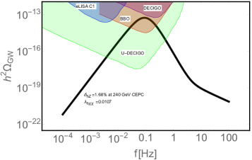
Considering the above discussion, we take one set of benchmark points , and . Then, the corresponding DM mass is 66 GeV, the pseudo scalar mass and the charged scalar mass are both 300 GeV, . Taking this set of benchmark points, the relic density, DM direct search, collider constraints and a strong FOPT can be satisfied simultaneously. Using the methods and formulae in the appendix, the phase transition GW signal is shown in Fig.1, which is just within the sensitivity of BBO and U-DICIGO. The colored regions represent the sensitivities of different GW experiments (DECIGO Moore:2014lga , eLISA Caprini:2015zlo , BBO, and U-DECIGO Kudoh:2005as ), and the black line corresponds to the GW signals, which also means the hZ cross section () deviation from the SM in 240 GeV circular electron-positron collider (CEPC). At the 240 GeV CEPC CEPC-SPPCStudyGroup:2015csa with an integrated luminosity of , the precision of could be about Gomez-Ceballos:2013zzn . And at the 240 GeV CEPC, the deviation of the hZ cross section at one-loop level Huang:2015izx is about Arhrib:2015hoa ; Kanemura:2016sos , which is well within the sensitivity of CEPC. The international linear collider (ILC) Gomez-Ceballos:2013zzn can also test this model. The GW signal and the hZ cross section deviation at future lepton collider can make a double test on the DM of IDM as shown in Fig. 1.
III Gravitational Waves in Mixed Dark Matters
We have discussed FOPT and GWs if there is only one single multiplet scalar dark matter in the dark sector. Due to the tight correlation between strong FOPT and the DM direct detection, only the IDM is viable for strong FOPT and detectable GWs. Based on the relic density requirement, the IDM has very limited viable parameter region: GeV, and the blind spot region . In this section, we would like to extend the single DM multiplet models into the mixed scalar DM models.
The mixed scalar DM scenario involves in several -odd scalar multiplets in the dark sector, which could be mixed. The simplest models involve in two dark matter multiplets: the mixed singlet-doublet model (MSDM) and the mixed singlet-triplet model (MSTM) Fischer:2013hwa ; Cheung:2013dua . Compared to the single scalar DM, the advantages of the mixed DM scenario are
-
•
It is easy to obtain a large blind spot region, at which the DM-Higgs coupling is zero.;
-
•
If the DM is mixture of a singlet and multiplet (well-tempered), the relic density could be realized in a large DM mass range;
-
•
There are more degree of freedoms which contribute to the thermal barriers of the electroweak phase transition.
From the above, we note that it is necessary to have a singlet component to reduce the large annihilation cross section during freeze-out. The higher multiplet is also tightly constrained by the plasma screening and Higgs diphoton constraints.
We will focus on the strong FOPT and GWs in the blind spot region with broad DM mass range in the MSDM and MSTM. Here, we adapt the effective Lagrangian in Ref. Cheung:2013dua . Denote the SM singlet as and the neutral component of the multiplet as . Due to the mixing between two fields, the mass eigenstates have
| (13) | |||||
| (14) |
The effective Lagrangian for the mass eigenstates has
| (15) |
Define the dimensionless coupling and . According to Ref. Cheung:2013dua , the mixed DM scenario could have large viable parameter region after imposing the direct detection constraints and requirement on the DM relic abundance. Unlike the IDM, the DM mass could be arbitrary. The viable parameter region strongly depends on two parameters: the , and the mixing angle . The spin-independent direct detection rate is dominated by the Higgs exchange with the cross section:
| (16) |
Thus, the needs to be small to avoid tight direct detection constraints. In this study, we take the blind spot region: . The dominant thermal annihilation channels could be very different and distinct depending on the DM mass region. To produce detectable GW signature, we would like to focus on the moderate DM mass region ( GeV) 555Of course, the parameter space near the Higgs funnel region is also viable. But we focus on a broader parameter region in this work.. The dominant annihilation channels are
-
•
the -channel annihilations: , in which the annihilation rate depends on the ;
-
•
the contact four point annihilation: for real multiplet and for doublet;
-
•
the -channel annihilation: via exchanging of the charged scalars;
Given in the blind spot region, we assume that the contact and -channel annihilation processes are dominant 666 There is still small parameter region in which the -channel and gauge interactions have interference effects.. In this case, the annihilation cross sections only depend on the gauge interactions, and the annihilation rate near the blind spot region is greatly simplified as
| (17) |
for the mixed singlet-doublet, and
| (18) |
for the mixed singlet-triplet model. To obtain the required relic abundance, the mixing angle needs to satisfy
| (19) | |||||
| (20) |
which could be deduced from Ref. Cirelli:2005uq ; Hambye:2009pw . Note that this simple relation is only valid near the blind spot region. In the interested mass region ( GeV), the well-tempered DM is favored. Therefore, we could choose the benchmark points by acquiring is close to zero (blind spots) and is determined by the above Eq. (20). Using these two conditions, we could obtain correct relic abundance, while escaping the DM direct detection constraints and obtaining a strong FOPT with detectable GWs.
III.1 The Mixed Singlet-Doublet Model
The MSDM contains a singlet with hypercharge , and a doublet with hypercharge . The tree level potential in the MSDM is
Here, we omit all interactions involving only and and the kinetic terms. The mixed mass matrices are
| (23) |
where and . The two eigenvalues of the mass-squared matrix are
| (24) |
with the smaller eigenvalue corresponding to DM mass square
| (25) |
The mixing angle is
| (26) |
The coupling between the Higgs boson and DM is
and the coupling between the Higgs boson and the singlet scalar is
In the DM favored parameter spaces (small , GeV and GeV), a strong FOPT can be induced due to the fact that the strong FOPT can occur in the IDM and the mixing with an inert singlet can enhance the FOPT. The mixing term does not significantly change the phase transition property except for the change of the eigenvalues of the masses. Taking the same approximations as in the IDM and writing in the forms of Eq.(8), we have . The strong FOPT can be easily realized if and are order one which are allowed by the above DM constraints.
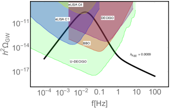
We take one set of benchmark points , , , , and . Then, we have , and . The corresponding GW spectra are shown in Fig.2. This set of benchmark points can evade the constraints from DM direct experiments, give the correct relic density and produce detectable GW signals by eLISA, BBO, DECIGO and U-DECIGO. We estimate the deviation of the hZ cross section at one-loop level is about Arhrib:2015hoa ; Kanemura:2016sos at the 240 GeV CEPC, which is well within the sensitivity of CEPC and ILC. As for the precise prediction on the collider signals at the CEPC and ILC in this MSDM model, we leave it in our future study.
III.2 The Mixed Singlet-Triplet Model
Similarly, the MSTM contains a real singlet and a real triplet with . The relevant potential in the MSTM is
| (29) | |||||
The coupling between the Higgs boson and DM is
with the DM mass square
| (31) |
where and . The coupling between the Higgs boson and the singlet is
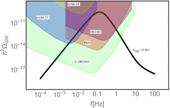
Taking the same approximations as in the above discussions, we have . In the MSTM, we take the set of benchmark points , , GeV, . Then, we have , and . The GW spectrum is shown in Fig.3, which is within the sensitivity of the BBO, eLISA, DECIGO and U-DECIGO. We also leave the study of collider signals in the MSTM in our future study.
IV Conclusion
We have investigated the GW signatures associated with the possible strong FOPT in the early universe in a generic class of inert scalar multiplet DM models. We have found that there is usually a strong tension between the strength of the phase transition and the DM direct detection, except the blind spot region with narrow DM mass range in the IDM. In the IDM, we have shown that although the direct detection experiments could not probe the blind spot region, at which the Higgs-DM coupling is zero, the GW detection and lepton colliders could help us further explore the parameter space which cannot be addressed by the DM searches.
To enlarge the blind spot region with broader DM mass range, we considered the mixed scalar DM scenario. We focused on the minimal singlet-doublet dark matter and minimal singlet-triplet DM models, and showed that the blind spot region in these models could avoid all the relevant constraints, have required relic density, and produce strong FOPT in the early universe. The GW signatures are explored in this scenario, and we found that the blind spot region could be further explored via the GW signatures and collider signatures in future. This provides us a new way to detect the DM in future. And our strategy could also be used to more general DM scenarios than the scalar multiplet DM models. We expect the future GW and collider experiments, such as eLISA and TianQin Luo:2015ght , CEPC and ILC, could probe these DM scenarios beyond the reaches of the DM direct detection experiments.
Acknowledgements
JHY was supported in part under U.S. Department of Energy contract DE-SC0011095. FPH was supported in part by the NSFC (Grant Nos. 11121092, 11033005, 11375202) and by the CAS pilotB program. FPH was also supported by the China Postdoctoral Science Foundation under Grant No. 2016M590133.
Appendix
In this appendix, the details on the calculation of phase transition GW spectrum are shown. In general, there exist three mechanisms to produced phase transition GWs: the first one is the well-known bubble collisions Kamionkowski:1993fg , the second one is the turbulence in the fluid, where a certain fraction of the bubble walls energy is converted into turbulence Kosowsky:2001xp ; Caprini:2009yp , and the last one is the new mechanism of sound waves Hindmarsh:2013xza .
When a strong FOPT occurs, via thermally fluctuating or quantum tunneling the potential barrier, bubbles are nucleated with the nucleation rate per unit volume and Linde:1981zj . The Euclidean action Coleman:1977py ; Callan:1977pt , and then Linde:1981zj where
| (33) |
Thus, the bubble nucleation rate can be obtained Cai:2017cbj by calculating the profile of the scalar field through solving the following bounce equation:
| (34) |
with the boundary conditions and . The phase transition terminates if it satisfies
| (35) |
The phase transition GW spectrum depends on four parameters. The first parameter is , where is determined by Eq.(35). The false vacuum energy (latent heat) density , and the plasma thermal energy density . The parameter represents the strength the FOPT, namely, a larger value of produces stronger GW signature. The second parameter is , where one has , namely, corresponds to the typical time scale of the phase transition. The third parameter is the efficiency factor (i=co,tu,sw), and the last parameter is the bubble wall velocity .
Once the four parameters are known, the corresponding phase transition GWs in the three mechanisms can be directly obtained after considering the red-shift effects . The current peak frequency at each mechanism is with i=co,tu,sw, respectively. In the bubble collision mechanism, the GW spectrum is expressed as Huber:2008hg
with the peak frequency Huber:2008hg at . In the turbulence mechanism, the GW signals have the peak frequency at about at Caprini:2015zlo , and the phase transition GW intensity is formulated by Caprini:2009yp ; Binetruy:2012ze
In the sound wave mechanism, the GW spectrum can be written as Hindmarsh:2013xza ; Caprini:2015zlo
with the peak frequency at Hindmarsh:2013xza ; Caprini:2015zlo , where for relativistic bubbles Espinosa:2010hh .
References
- (1) B. P. Abbott et al. [LIGO Scientific and Virgo Collaborations], Phys. Rev. Lett. 116, no. 6, 061102 (2016) [arXiv:1602.03837 [gr-qc]].
- (2) E. Witten, Phys. Rev. D 30, 272 (1984).
- (3) C. J. Hogan, Phys. Lett. B 133, 172 (1983); C. J. Hogan, Mon. Not. Roy. Astron. Soc. 218, 629 (1986).
- (4) M. S. Turner and F. Wilczek, Phys. Rev. Lett. 65, 3080 (1990).
- (5) M. Kamionkowski, A. Kosowsky and M. S. Turner, Phys. Rev. D 49, 2837 (1994) [astro-ph/9310044].
- (6) M. Hindmarsh, S. J. Huber, K. Rummukainen and D. J. Weir, Phys. Rev. Lett. 112, 041301 (2014) [arXiv:1304.2433 [hep-ph]];
- (7) A. Kosowsky, A. Mack and T. Kahniashvili, Phys. Rev. D 66, 024030 (2002) [astro-ph/0111483].
- (8) C. Caprini, R. Durrer and G. Servant, JCAP 0912, 024 (2009) [arXiv:0909.0622 [astro-ph.CO]].
- (9) M. Hindmarsh, S. J. Huber, K. Rummukainen and D. J. Weir, Phys. Rev. D 92, 123009 (2015) [arXiv:1504.03291 [astro-ph.CO]].
- (10) F. P. Huang, Y. Wan, D. G. Wang, Y. F. Cai and X. Zhang, Phys. Rev. D 94, no. 4, 041702 (2016) doi:10.1103/PhysRevD.94.041702 [arXiv:1601.01640 [hep-ph]].
- (11) J. Jaeckel, V. V. Khoze and M. Spannowsky, Phys. Rev. D 94, no. 10, 103519 (2016) doi:10.1103/PhysRevD.94.103519 [arXiv:1602.03901 [hep-ph]].
- (12) P. S. B. Dev and A. Mazumdar, Phys. Rev. D 93, no. 10, 104001 (2016) doi:10.1103/PhysRevD.93.104001 [arXiv:1602.04203 [hep-ph]].
- (13) K. Hashino, M. Kakizaki, S. Kanemura and T. Matsui, Phys. Rev. D 94, no. 1, 015005 (2016) doi:10.1103/PhysRevD.94.015005 [arXiv:1604.02069 [hep-ph]].
- (14) R. Jinno and M. Takimoto, Phys. Rev. D 95, no. 1, 015020 (2017) doi:10.1103/PhysRevD.95.015020 [arXiv:1604.05035 [hep-ph]].
- (15) H. Yu, B. M. Gu, F. P. Huang, Y. Q. Wang, X. H. Meng and Y. X. Liu, JCAP 1702, 039 (2017) doi:10.1088/1475-7516/2017/02/039 [arXiv:1607.03388 [gr-qc]].
- (16) A. Kobakhidze, A. Manning and J. Yue, arXiv:1607.00883 [hep-ph].
- (17) P. Huang, A. J. Long and L. T. Wang, Phys. Rev. D 94, no. 7, 075008 (2016) doi:10.1103/PhysRevD.94.075008 [arXiv:1608.06619 [hep-ph]].
- (18) M. Artymowski, M. Lewicki and J. D. Wells, JHEP 1703, 066 (2017) doi:10.1007/JHEP03(2017)066 [arXiv:1609.07143 [hep-ph]].
- (19) A. Soni and Y. Zhang, arXiv:1610.06931 [hep-ph].
- (20) C. Balazs, A. Fowlie, A. Mazumdar and G. White, Phys. Rev. D 95, no. 4, 043505 (2017) doi:10.1103/PhysRevD.95.043505 [arXiv:1611.01617 [hep-ph]].
- (21) G. C. Dorsch, S. J. Huber, T. Konstandin and J. M. No, arXiv:1611.05874 [hep-ph].
- (22) F. P. Huang and X. Zhang, arXiv:1701.04338 [hep-ph].
- (23) W. Chao, H. K. Guo and J. Shu, arXiv:1702.02698 [hep-ph].
- (24) A. Beniwal, M. Lewicki, J. D. Wells, M. White and A. G. Williams, arXiv:1702.06124 [hep-ph].
- (25) A. Addazi and A. Marciano, arXiv:1703.03248 [hep-ph].
- (26) L. Marzola, A. Racioppi and V. Vaskonen, arXiv:1704.01034 [hep-ph].
- (27) L. Bian, H. K. Guo and J. Shu, arXiv:1704.02488 [hep-ph].
- (28) A. Tan et al. [PandaX-II Collaboration], Phys. Rev. Lett. 117, no. 12, 121303 (2016) doi:10.1103/PhysRevLett.117.121303 [arXiv:1607.07400 [hep-ex]].
- (29) D. S. Akerib et al. [LUX Collaboration], Phys. Rev. Lett. 118, no. 2, 021303 (2017) doi:10.1103/PhysRevLett.118.021303 [arXiv:1608.07648 [astro-ph.CO]].
- (30) J. R. Espinosa, T. Konstandin, J. M. No and M. Quiros, Phys. Rev. D 78, 123528 (2008) doi:10.1103/PhysRevD.78.123528 [arXiv:0809.3215 [hep-ph]].
- (31) T. A. Chowdhury, M. Nemevsek, G. Senjanovic and Y. Zhang, JCAP 1202, 029 (2012) doi:10.1088/1475-7516/2012/02/029 [arXiv:1110.5334 [hep-ph]].
- (32) P. Schwaller, Phys. Rev. Lett. 115, 181101 (2015) [arXiv:1504.07263 [hep-ph]].
- (33) P. A. Seoane et al. [eLISA Collaboration], arXiv:1305.5720 [astro-ph.CO].
- (34) V. Corbin and N. J. Cornish, Class. Quant. Grav. 23, 2435 (2006) [gr-qc/0512039].
- (35) N. Seto, S. Kawamura and T. Nakamura, Phys. Rev. Lett. 87, 221103 (2001) doi:10.1103/PhysRevLett.87.221103 [astro-ph/0108011].
- (36) H. Kudoh, A. Taruya, T. Hiramatsu and Y. Himemoto, Phys. Rev. D 73, 064006 (2006) [gr-qc/0511145].
- (37) M. Cirelli, N. Fornengo and A. Strumia, Nucl. Phys. B 753, 178 (2006) doi:10.1016/j.nuclphysb.2006.07.012 [hep-ph/0512090].
- (38) T. Hambye, F.-S. Ling, L. Lopez Honorez and J. Rocher, JHEP 0907, 090 (2009) Erratum: [JHEP 1005, 066 (2010)] doi:10.1007/JHEP05(2010)066, 10.1088/1126-6708/2009/07/090 [arXiv:0903.4010 [hep-ph]].
- (39) O. Fischer and J. J. van der Bij, JCAP 1401, 032 (2014) doi:10.1088/1475-7516/2014/01/032 [arXiv:1311.1077 [hep-ph]].
- (40) C. Cheung and D. Sanford, JCAP 1402, 011 (2014) doi:10.1088/1475-7516/2014/02/011 [arXiv:1311.5896 [hep-ph]].
- (41) E. Ma, Phys. Rev. D 73, 077301 (2006) doi:10.1103/PhysRevD.73.077301 [hep-ph/0601225].
- (42) R. Barbieri, L. J. Hall and V. S. Rychkov, Phys. Rev. D 74, 015007 (2006) doi:10.1103/PhysRevD.74.015007 [hep-ph/0603188].
- (43) A. Belyaev, G. Cacciapaglia, I. P. Ivanov, F. Rojas and M. Thomas, arXiv:1612.00511 [hep-ph].
- (44) C. P. Burgess, M. Pospelov and T. ter Veldhuis, Nucl. Phys. B 619, 709 (2001) doi:10.1016/S0550-3213(01)00513-2 [hep-ph/0011335].
- (45) P. Fileviez Perez, H. H. Patel, M. J. Ramsey-Musolf and K. Wang, Phys. Rev. D 79, 055024 (2009) doi:10.1103/PhysRevD.79.055024 [arXiv:0811.3957 [hep-ph]].
- (46) S. S. AbdusSalam and T. A. Chowdhury, JCAP 1405, 026 (2014) doi:10.1088/1475-7516/2014/05/026 [arXiv:1310.8152 [hep-ph]].
- (47) D. Borah and J. M. Cline, Phys. Rev. D 86, 055001 (2012) doi:10.1103/PhysRevD.86.055001 [arXiv:1204.4722 [hep-ph]].
- (48) G. Gil, P. Chankowski and M. Krawczyk, Phys. Lett. B 717, 396 (2012) doi:10.1016/j.physletb.2012.09.052 [arXiv:1207.0084 [hep-ph]].
- (49) N. Blinov, S. Profumo and T. Stefaniak, JCAP 1507, no. 07, 028 (2015) doi:10.1088/1475-7516/2015/07/028 [arXiv:1504.05949 [hep-ph]].
- (50) M. Laine, M. Meyer and G. Nardini, arXiv:1702.07479 [hep-ph].
- (51) D. J. H. Chung, A. J. Long and L. T. Wang, Phys. Rev. D 87, no. 2, 023509 (2013) doi:10.1103/PhysRevD.87.023509 [arXiv:1209.1819 [hep-ph]].
- (52) P. A. R. Ade et al. [Planck Collaboration], Astron. Astrophys. 594, A13 (2016) doi:10.1051/0004-6361/201525830 [arXiv:1502.01589 [astro-ph.CO]].
- (53) C. J. Moore, R. H. Cole and C. P. L. Berry, Class. Quant. Grav. 32, 015014 (2015) [arXiv:1408.0740 [gr-qc]].
- (54) C. Caprini et al., JCAP 1604, no. 04, 001 (2016) doi:10.1088/1475-7516/2016/04/001 [arXiv:1512.06239 [astro-ph.CO]].
- (55) CEPC-SPPC Study Group, IHEP-CEPC-DR-2015-01, IHEP-TH-2015-01, IHEP-EP-2015-01.
- (56) M. Bicer et al. [TLEP Design Study Working Group Collaboration], JHEP 1401, 164 (2014) [arXiv:1308.6176 [hep-ex]].
- (57) F. P. Huang, P. H. Gu, P. F. Yin, Z. H. Yu and X. Zhang, Phys. Rev. D 93, no. 10, 103515 (2016) doi:10.1103/PhysRevD.93.103515 [arXiv:1511.03969 [hep-ph]].
- (58) A. Arhrib, R. Benbrik, J. El Falaki and A. Jueid, JHEP 1512, 007 (2015) doi:10.1007/JHEP12(2015)007 [arXiv:1507.03630 [hep-ph]].
- (59) S. Kanemura, M. Kikuchi and K. Sakurai, Phys. Rev. D 94, no. 11, 115011 (2016) doi:10.1103/PhysRevD.94.115011 [arXiv:1605.08520 [hep-ph]].
- (60) J. Luo et al. [TianQin Collaboration], Class. Quant. Grav. 33, no. 3, 035010 (2016) doi:10.1088/0264-9381/33/3/035010 [arXiv:1512.02076 [astro-ph.IM]].
- (61) A. D. Linde, Nucl. Phys. B 216, 421 (1983) Erratum: [Nucl. Phys. B 223, 544 (1983)]. doi:10.1016/0550-3213(83)90293-6, 10.1016/0550-3213(83)90072-X
- (62) S. R. Coleman, Phys. Rev. D 15, 2929 (1977) Erratum: [Phys. Rev. D 16, 1248 (1977)]. doi:10.1103/PhysRevD.15.2929, 10.1103/PhysRevD.16.1248
- (63) C. G. Callan, Jr. and S. R. Coleman, Phys. Rev. D 16, 1762 (1977). doi:10.1103/PhysRevD.16.1762
- (64) R. G. Cai, Z. Cao, Z. K. Guo, S. J. Wang and T. Yang, arXiv:1703.00187 [gr-qc].
- (65) S. J. Huber and T. Konstandin, JCAP 0809, 022 (2008) [arXiv:0806.1828 [hep-ph]].
- (66) P. Binetruy, A. Bohe, C. Caprini and J. F. Dufaux, JCAP 1206, 027 (2012) [arXiv:1201.0983 [gr-qc]].
- (67) J. R. Espinosa, T. Konstandin, J. M. No and G. Servant, JCAP 1006, 028 (2010) [arXiv:1004.4187 [hep-ph]].