The hottest hot Jupiters may host atmospheric dynamos

Abstract

Hot Jupiters have proven themselves to be a rich class of exoplanets which test our theories of planetary evolution and atmospheric dynamics under extreme conditions. Here, we present three-dimensional magnetohydrodynamic simulations and analytic results which demonstrate that a dynamo can be maintained in the thin, stably-stratified atmosphere of a hot Jupiter, independent of the presumed deep-seated dynamo. This dynamo is maintained by conductivity variations arising from strong asymmetric heating from the planets’ host star. The presence of a dynamo significantly increases the surface magnetic field strength and alters the overall planetary magnetic field geometry, possibly affecting star-planet magnetic interactions.

1 Introduction

To date more than 5000 exoplanets have been discovered and a couple hundred are considered “hot Jupiters” – Jupiter sized planets close to their host star. Hot Jupiters were the first detected exoplanets and remain the best characterized due to their favorable observing conditions. Because of their close proximity to their host star, these planets are tidally locked with a constant day and nightside. This asymmetric heating leads to strong eastward directed atmospheric winds which have been studied extensively (Cho et al., 2003; Showman & Guillot, 2002; Cooper & Showman, 2005; Dobbs-Dixon & Lin, 2008; Showman et al., 2009; Rauscher & Menou, 2010; Lewis et al., 2010; Thrastarson & Cho, 2010; Heng et al., 2011; Kataria et al., 2016). While atmospheric dynamic calculations generally yield similar results, such as eastward winds in excess of a km/s, observations indicate varying circulation efficiency. Infrared observations have demonstrated that hot Jupiters have a range of day-night temperature differentials and there is some indication that this variation is temperature dependent, with hotter planets showing larger differentials than cooler planets (Cowan & Agol, 2011; Komacek & Showman, 2016).

Intense irradiation from the host star can lead to thermal ionization of several alkali metals (Perna et al., 2010a; Batygin & Stevenson, 2010). Therefore, hot Jupiters are partially ionized. Numerous authors have demonstrated that this ionization allows atmospheric winds to couple to the deep-seated, dynamo driven magnetic field (Perna et al., 2010a, b; Batygin & Stevenson, 2010; Menou, 2012a). This coupling could lead to currents which penetrate into the deep atmosphere, generating Ohmic heating, which could in turn, contribute to the inflated radii observed in half of all hot Jupiters (Batygin et al., 2011; Wu & Lithwick, 2013; Ginzburg & Sari, 2015, 2016). Magnetic interaction could also reduce circulation efficiency, particularly in hot planets where the day-night flow could be impeded by the Lorentz force. These results demonstrate that magnetism in hot Jupiters could have important observational consequences and thus, warrant further investigation.

Rogers & Showman (2014) carried out the fist magnetohydrodynamic (MHD) simulations of a hot Jupiter which self-consistently included Ohmic heating. Those simulations found that inclusion of magnetic fields could severely affect the atmospheric flows leading to variable and reversed winds. They also found that while the MHD simulations did reproduce the qualitative picture proposed by earlier theoretical work (Menou, 2012a; Rauscher & Menou, 2013), they failed to reproduce the amplitude of Ohmic heating required to explain inflated radii (Rogers & Showman, 2014; Rogers & Komacek, 2014). The discrepancy between theoretical models and numerical simulations leaves the viability of the Ohmic mechansim for inflating exoplanets still in question.

Hot Jupiters also likely interact with their host stars’ magnetic field, possibly leading to observable features such as asymmetry in the light curves of transiting planets (Vidotto et al., 2010; Cauley, 2015) and induced activity in the atmosphere of their host star (Shkolnik et al., 2003a, b, 2005). Such interactions depend on the planetary magnetic field strength and geometry (Cuntz et al., 2000; Ip et al., 2004). Therefore, understanding the planetary magnetic field is important if we are to correctly interpret such observations.

The day-night temperature differential on hot Jupiters leads to severe day-night variations in ionization and hence, conductivity. Similarly, there are large variations in conductivity between deep and shallow atmospheric layers. Busse & Wicht (1992) showed that variations in conductivity in the direction of the dominant flow, could lead to a dynamo. More recently, Petrelis et al. (2016) showed that a temperature dependent conductivity could produce a dynamo, even with small temperature fluctuations and a weakly temperature-dependent conductivity. Hot Jupiter atmospheres are perhaps the most asymmetric astrophysical objects, with perhaps the largest temperature (conductivity) variations and so provide an ideal testbed of the theories outlined in those works. Here we present three-dimensional (3D) numerical simulations and analytic results which show that a variable conductivity dynamo (VCD) may proceed in some hot Jupiter atmospheres.

2 Numerical simulations of atmospheric dynamos

We solve the full magnetohydrodynamic (MHD) equations in 3D in the anelastic approximation, as described in Rogers & Komacek (2014). The model solves the following equations:

$$\mathbf{\nabla}\cdot{\bar{\rho}}{\bf v} = 0,$$ (1)

$$\mathbf{\nabla}\cdot\mathbf{B} = 0,$$ (2)

$${\bar{\rho}}\frac{\partial\mathbf{v}}{\partial t}+\mathbf{\nabla}\cdot({\bar{\rho}}\mathbf{v}\mathbf{v}) = -{\bf\nabla}p-\rho{\bar{g}}{\hat{\bf r}}+2{\bar{\rho}}{\bf v}\times{\bf\Omega}+\ldots$$ (3)

$$\mbox{}+\mathbf{\nabla}\cdot\left[2{\bar{\rho}}{\bar{\nu}}\left(e_{ij}-\frac{1}{3}\delta_{ij}\,(\mathbf{\nabla}\cdot\mathbf{v})\right)\right]-\frac{1}{\mu_{0}}\mathbf{B}\times({\bf\nabla}\times\mathbf{B}),$$

$${\frac{\partial{T}}{\partial{t}}}+(\mathbf{v}\cdot\nabla){T} = -v_{r}\left[{\frac{\partial{\overline{T}}}{\partial{r}}}-(\gamma-1)\overline{T}h_{\rho}\right]+(\gamma-1)Th_{\rho}v_{r}+\ldots$$ (4)

$$\mbox{}+\gamma\overline{\kappa}\left[\nabla^{2}T+(h_{\rho}+h_{\kappa}){\frac{\partial{T}}{\partial{r}}}\right]+\frac{T_{eq}-T}{\tau_{rad}}+\frac{\eta}{\mu_{o}\rho c_{p}}|\nabla\times\mathbf{B}|^{2}.$$

Equation 1 represents the continuity equation in the anelastic approximation (Gough, 1969; Rogers & Glatzmaier, 2005). This approximation allows some level of compressibility by allowing variation of the reference state density, ${\bar{\rho}}$, which varies in this model by four orders of magnitude. Equation 2 represents the conservation of magnetic flux. Equation 3 represents conservation of momentum including Coriolis and Lorentz forces. Equation 4 represents the energy equation including a forcing term to mimic stellar insolation (fourth term on right hand side) and Ohmic heating (fifth term on right hand side, where T_eq is defined in Equation 6). All variables take their usual meaning and details can be found in Rogers & Komacek (2014).

In the work presented here, the magnetic diffusivity $\eta$ (inverse conductivity) is a function of all space. Therefore, the magnetic induction equation is

$${\partial{\bf B}\over\partial t}=\nabla\times\left({\bf v}\times{\bf B}\right)+\eta\nabla^{2}{\bf B}-\left(\nabla\eta\right)\times\left(\nabla\times{\bf B}\right).$$ (5)

In the hot Jupiter system toroidal field can be generated from poloidal field by radial shear due to stronger winds at the planetary surface. Although the dynamo mechanism by conductivity variations is subtle, one can show that given the correct alignment between $\nabla\times{\bf B}$ and $\nabla\eta$ the last term on the right hand side (RHS) of Equation 5 can provide a positive $\alpha$ effect, thus regenerating poloidal field from toroidal and closing the dynamo loop.

The magnetic diffusivity is calculated from the initial temperature profile given by:

$$T_{eq}\left(r,\theta,\phi\right)={\overline{T}}(r)+\Delta T_{eq}(r),\cos\theta\cos\phi$$ (6)

where ${\overline{T}}(r)$ is the reference state temperature from (Rogers & Komacek, 2014) and $\Delta T_{eq}$ is the specified day-night temperature, which is extrapolated logarithmically from the surface to 10 Bar. Using this temperature profile, the magnetic diffusivity is calculated using the method from Rauscher & Menou (2013) where:

$$\eta\left(r,\theta,\phi\right)=230\frac{\sqrt{T_{eq}}}{\chi_{e}}$$ (7)

and $\chi_{e}$ is the ionization fraction. The ionization fraction is calculated at each point using the Saha equation taking into account all elements from hydrogen to nickel and abundances from Lodders (2010).

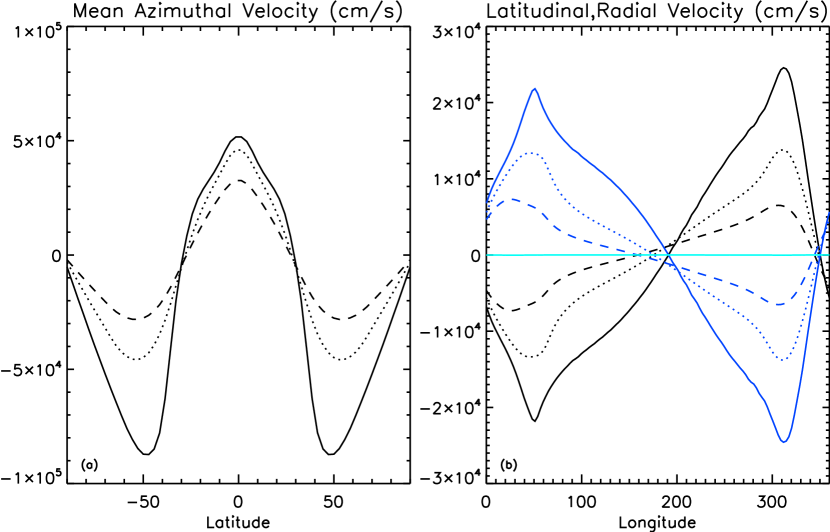
Figure 1: Atmospheric winds in hot Jupiter atmosphere. (a) Time and longitudinally averaged longitudinal velocity at the surface (solid line), 95% (dotted line) and 85% of the computed domain (dashed line). (b) Latitudinal velocity averaged in time and over the Northern/Southern hemispheres (blue/black lines respectively) at the same depths as (a). Similarly averaged radial velocities are shown in cyan. (c) Time and longitudinally averaged velocity as a function of radius at the equator (solid line) and at mid-latitudes (dashed and dotted line).

The fiducial numerical model we present is Model M8 from Rogers & Komacek (2014), but with $\Delta T_{eq}$=1000 K, such that the night side at the top of the domain is $\sim$1800 K and the day side is $\sim$2800 K. The atmospheric winds found in the hydrodynamic model are shown in Fig. 1. Near the surface, where the temperature forcing is strong, the model produces strong eastward directed jets at low latitudes, return flows at high latitudes and weaker, hemispheric meridional circulation. Deeper in the atmosphere, the forcing is reduced and winds fall off dramatically with depth. Radial flows are extremely weak throughout, with amplitudes 0.1–1% their horizontal counterparts. These winds are similar to those found in many other hydrodynamical simulations of hot Jupiters (Cooper & Showman, 2005), with the main difference being that our winds are slightly weaker, probably due to the use of the full viscous term, rather than using a hyperdiffusivity.

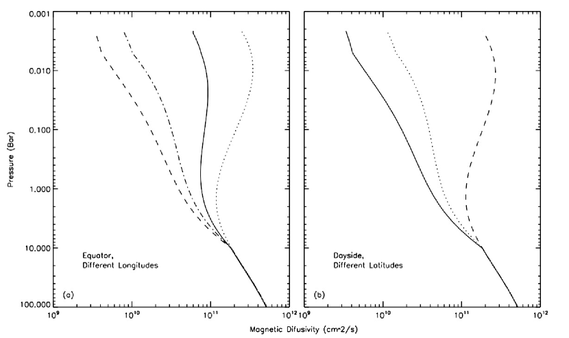
Figure 2: Profile of magnetic diffusivity as a function of longitude (a) and latitude (b). (a) Radial profile of diffusivity at the equator at the sub-stellar point (dashed line), the nightside (dotted line), near the terminator (dash-dot line) and the mean (solid line). (b) Radial profile of diffusivity at the substellar point at the equator (solid line), mid-latitude (dotted line) and near the pole (dashed line).

Magnetic effects are then investigated by including an initial magnetic field of 5 G at the bottom and 3 G at the top of the domain. Fig. 2 shows the magnetic diffusivity as a function of radius for various latitudes and longitudes for our model. This “dynamo” model has no continously imposed field, unlike the models presented in Rogers & Showman (2014) and Rogers & Komacek (2014). However, to fully investigate the effect of an atmospheric dynamo, we ran three additional models: (1) “constant $\eta$” — a model with a constant magnetic diffusivity equal to the mean diffusivity ($5\times 10^{11}$), (2) “imposed+dynamo” — a model with variable conductivity, as shown in Fig. 2 but with an imposed dipolar magnetic field of strength 3 G at the base of the simulated domain meant to mimic the deep-seated, convectively driven dynamo and (3) “imposed+constant” — a model with an imposed dipolar magnetic field of strength 3 G at the base of the simulated domain, but with a constant magnetic diffusivity ($5\times 10^{11}$).

The magnetic diffusivity is not a function of time in any of the models. That is, it does not change due to advection of heat or Ohmic heating. We will include this effect in forthcoming papers, but discuss the possible relevance of a fully temperature-dependent conductivity in Section 5.

3 Numerical Results

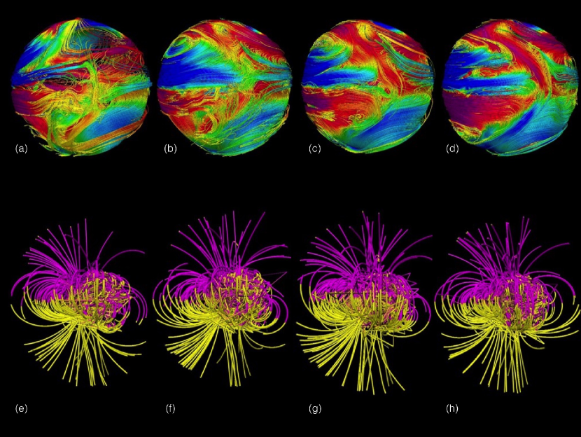
Figure 3: Time snapshots of toroidal (azimuthal) magnetic field (looking onto the terminator) (a–d) and the radial magnetic field (e–h).

The effect of the magnetic field on the atmospheric winds depends sensitively on the diffusivity profile and strength of the magnetic field, details of which can be found in Rogers & Komacek (2014). In the dynamo model presented here, the atmospheric winds are strongly coupled to the magnetic field and therefore, the winds become weaker and variable. A time snapshot of magnetic field lines for the “dynamo” model, is shown in Fig.3. The top row shows magnetic field lines looking onto the terminator, color-coded by the azimuthal field strength, with blue positive and magenta negative. Magnetic field is swept from the dayside, where field and flow are strongly coupled, to the nightside, where much of this field is dissipated. The collision between the strongly coupled field on the dayside and the weakly coupled field on the nightside leads to complex field topology and magnetic energy generation. This interaction particularly generates strong latitudinal field at the terminator, as can be seen in Fig. 3d.

Investigation of (5), shows that the VCD $\alpha$ effect is $\propto{\bf J}\times{\bf\nabla}\eta$. The current, ${\bf J}$, is strongly correlated with vorticity, which tends to be strongest at the day-night terminator and on the nightside (Rogers & Komacek, 2014). The terminator is also where conductivity gradients are large, hence in this region the necessary conditions for a dynamo are satisfied. Specifically, we find that the radial component of the magnetic field is regenerated predominantly from the azimuthal diffusivity gradient $\sim{\bf\nabla}\eta_{\phi}J_{\theta}$ and the latitudinal component is regenerated predominantly from the radial diffusivity gradient $\sim{\bf\nabla}\eta_{r}J_{\phi}$. The azimuthal component of the magnetic field is regenerated by both the typical $\Omega$ effect and by radial gradients in magnetic diffusivity, $\sim{\bf\nabla}\eta_{r}J_{\theta}$. The presence of a dynamo is confirmed in Fig. 4 which shows the ratio of the magnetic to kinetic energy as a function of time for the “dynamo model” (solid line) and the “constant $\eta$” model (dash-dot line-drops so precipitously it can barely be seen in bottom left corner).

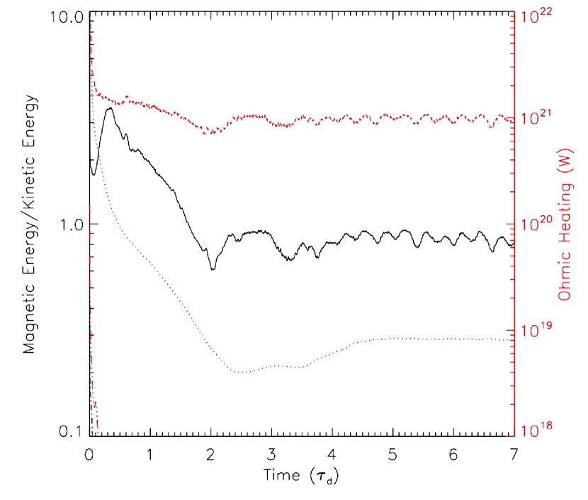
Figure 4: Magnetic energy and Ohmic heating as a function of time, displayed in diffusion times, using the mean diffusivity $10^{11}$ cm² s^-1. The left hand axis shows the ratio of magnetic to kinetic energy (solid black line), clearly showing a dynamo as the magnetic energy is maintained against diffusion. The right hand axis shows Ohmic heating integrated below 10 Bar (dotted line) and over the whole layer (dashed line).

In the saturated state the magnetic energy generation is balanced with Ohmic heating, which we also show in Fig. 4. If we compare the Ohmic heating here to the values obtained in Rogers & Komacek (2014) for a 3 G imposed field (see their Table 1) we see that the Ohmic heating here is equivalent to the Ohmic heating in a cooler model (between M6b3 and M7b3). Therefore, we conclude that the presence of a horizontally varying conductivity and the dynamo it produces, results in slightly lower overall Ohmic heating than one would expect from a model which does not consider a horizontally varying conductivity. This is likely because magnetic energy is maintaining the VCD, rather than being dissipated.

The bottom row of Fig. 3 shows the extrapolated field lines (out to 2R_p) for this model. There we see that the magnetic field is very asymmetric, with poloidal field concentrated predominantly on the dayside of the planet. Near the equator the surface poloidal field (defined as $B_{p}=\sqrt{B_{\theta}^{2}+B_{r}^{2}}$) is $\sim$15 G on the dayside of the planet and 7 G on the nightside of the planet. These values are 16 G/8 G for the “imposed+dynamo” model and $\sim$1 G on both the day and night side for the “imposed+constant” model. The inclusion of conductivity variations significantly increases the surface planetary field strength and leads to a highly asymmetric field. Therefore, unless the internal, convectively driven, magnetic field is particularly strong (in excess of 15 G at the surface), the surface planetary magnetic field is likely dominated by the magnetic field generated in the atmosphere, at least in hotter hot Jupiters.

The asymmetry in the field persists to $2R_{p}$ where about 65$\%$of the magnetic energy is found in the dipole component, 25$\%$ is in the $l=2$, $m=1$ component and 10$\%$ in the $l=3$, $m=2$ component, although by $4R_{p}$ the dipole component represents 95% of the total energy. However, these percentages fluctuate significantly in time. Such a complex field structure in space and time likely affects the SPMI expected in these close-in systems (Cuntz et al., 2000; Ip et al., 2004; Strugarek et al., 2015).

4 Analytic models of dynamo behavior in a hot Jupiter

The flow profile and conductivity variations in hot Jupiters are relatively simple, therefore, we attempt to solve this system analytically. While the diffusivity and initial velocity vary on a large scale in a hot Jupiter atmosphere, the magnetic energy is generated in a narrow region near the terminator. In that region the length scale of velocity and diffusivity variations is small. Therefore, we apply the standard technique of multiple scales from homogenization theory (Chiang & Vernescu, 2010) in 3D cartesian coordinates. This is a method for deriving an equation for the large scale variations in the magnetic field by averaging over the periodic small scale variations. We assume that the conductivity and velocity vary on a small spatial scale defined by a large wavenumber $k$ and define $\mathbf{X}=(X,Y,Z)=k\mathbf{x}$ and all functions must be periodic in $\mathbf{X}$. We then look for a solution of the form

$$\mathbf{B}=\mathbf{B}_{0}(t,\mathbf{x})+k^{-1}\mathbf{B}_{1}(t,\mathbf{x},\mathbf{X})+k^{-2}\mathbf{B}_{2}(t,\mathbf{x},\mathbf{X})+\cdots.$$ (8)

When we substituting (8) into (5) we get a series of equation at each order in $k$. The leading order equation, $O\left(k^{1}\right)$, gives an equation for $\mathbf{B}_{1}$ in terms of $\mathbf{B}_{0}$ and the $O\left(k^{0}\right)$ equation, after averaging over the periodic cell, gives an equation for $\mathbf{B}_{0}$. The $\mathbf{B}_{0}$ equation is

$$\nabla^{\prime}\times\left[(\eta(\nabla\times\mathbf{B}_{0}+\nabla^{\prime}\times\mathbf{B}_{1})-\mathbf{u}\times\mathbf{B}_{0}\right] = 0,$$ (9)

where $\nabla^{\prime}=(\partial_{X},\partial_{Y},\partial_{Z})$. This is to be contrasted with (4) in Petrelis et al. (2016), where there is no spatial variation in $\eta$ and a time derivative is included. We then write $\eta=\eta_{0}(1+\delta\eta^{\prime})$, where $\eta_{0}$ is constant, and $\eta^{\prime}$ varies between $\pm 1$, thus $\delta$ controls the strength of the variation in conductivity. Writing $\mathbf{B}_{1}=\sum_{k=0}\delta^{k}\mathbf{C}_{k}$ and Taylor expanding $(1+\delta\eta^{\prime})^{-1}$ we get a series of Poisson equations for $C_{k}$ which can be easily solved to give $\mathbf{B}_{1}$ in terms of $\mathbf{B}_{0}$ and $(\nabla\times\mathbf{B}_{0})$. This expansion is convergent for $\delta<1$, which we also expect on physical grounds since this corresponds to positive diffusivity everywhere.

We choose profiles similar to those found in hot Jupiters. Assuming $\hat{\mathbf{x}}$, $\hat{\mathbf{y}}$ and $\hat{\mathbf{z}}$ correspond to the azimuthal, latitudinal and radial directions, we write

$$\eta^{\prime}=\cos Z\sin X\sin Y,$$ (10)

and

$$\mathbf{u}=\sin Z\left(\hat{\mathbf{x}}U\sin X\cos Y+\hat{\mathbf{y}}V\cos X\sin Y\right)$$ (11)

Here $U$ and $V$ represent the azimuthal and meridional velocity amplitude, respectively. As discussed in Section 3 the winds in the hot Jupiter atmosphere are largely two-dimensional and are reasonably described by (11). Using the method described above we solve for $\mathbf{B}_{1}$ to $O(\delta^{4})$ and the $\mathbf{B}_{0}$ equation becomes

$$\frac{\partial\mathbf{B}_{0}}{\partial t}=\eta_{0}\left[1-\frac{\delta^{2}}{12}-\frac{\delta^{4}}{72}\right]\nabla^{2}\mathbf{B}_{0}+\eta_{0}\frac{\delta}{24}\left[1+\frac{\delta^{2}}{6}+\frac{233881}{3852288}\delta^{4}\right]\nabla\times\mathbf{B}_{0}^{\prime}+O(\delta^{6}),$$ (12)

where $\mathbf{B}_{0}^{\prime}=-VB_{x}\hat{\mathbf{x}}+UB_{y}\hat{\mathbf{y}}+(U-V)B_{z}\hat{\mathbf{z}}.$ The $\nabla\times\mathbf{B}_{0}^{\prime}$ term gives rise to the dynamo effect. When $UV>V^{2}$ (which is the appropriate case for hot Jupiters), the large scale magnetic field is unstable in the $\hat{\mathbf{x}}$ direction and the minimum critical Reynolds number, defined as $UL/\eta$ where L is the length scale of the large scale magnetic field, is

$$R_{mc}>\frac{\mbox{$\scriptstyle\sqrt{1+\sqrt{2}}$}\,(6-\delta^{2})(12+\delta^{2})}{\delta^{2}\left(6+\delta^{2}+\frac{233881}{642048}\delta^{4}\right)}.$$ (13)

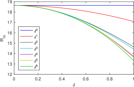
Figure 5: Scaled Critical Magnetic Reynolds number $\delta^{2}R_{mc}$ as a function of $\delta$ for different accuracies of $\mathbf{B}_{1}$ solution.

In hot Jupiters, the day-night diffusivity, $\eta_{max}/\eta_{min}=(1+\delta)/(1-\delta)$ varies between $\sim$10¹–$10^{4}$, which corresponds to a $\delta$ between 0.9–0.999. Figure 5 shows the approximate convergence of $R_{mc}(\delta)$ as $\delta$ approaches 1. If we take $\delta=0.9$ the $R_{mc}$ needed for instability is $\sim$14. Using the length scale over which magnetic energy is generated at the terminator ($\sim$10¹⁰ cm) and a typical velocity of $\sim$10⁴ cm s^-1, we conclude that in order for a hot Jupiter atmosphere to host a dynamo, the nightside magnetic diffusivity must be $\lesssim$10¹²–$10^{13}$ cm² s^-1, or a temperature of roughly 1400 K on the nightside of the planet. We expect the estimate for the diffusivity could vary by about an order of magnitude due to variations in metallicity and the inclusion of a temperature dependent diffusivity. Therefore, we conclude that a VCD only occurs in the hotter hot Jupiter atmospheres.

5 Discussion

Using numerical simulations coupled with analytic results we have shown that hot Jupiters with night side temperatures which are above $\sim$1400 K could host dynamos driven by spatial conductivity variations due to asymmetric heating from the host star. Lower temperatures and weak day-night temperature differentials do not produce dynamos. This is remarkable, not just because the dynamo is driven by conductivity variations (as has been shown previously), but also because it is maintained in a stably-stratified, thin atmosphere. The inclusion of horizontal variations in conductivity reduces Ohmic heating compared to a similar temperature object with no such variations. However, it is hard to make a direct comparison because of the large conductivity variations. To really investigate Ohmic heating, the analysis presented here will have to be done for a host of planetary temperatures and day-night temperature differences, something which is currently underway. Moreover, one needs to include the recovered Ohmic heating in a planetary evolution model to make a more concrete statement about the viability of Ohmic heating in explaining hot Jupiter radii. Finally, we will have to consider the interaction of the atmospheric field with the convectively generated field.

Whatever the deep seated field, it will be subject to interaction with the atmospheric winds and the variable conductivity in the atmosphere, both of which affect the overall field strength and geometry. We find that, unless the deep seated dynamo magnetic field is unreasonably strong, the surface planetary magnetic field strength is dominated by the induced field, particularly on the dayside of the planet. We also find that the magnetic field geometry is asymmetric, with dayside fields approximatley two times larger than their nightsides (dependent on the day-night temperature difference). Furthermore, we find that the energy in the dipole component of the magnetic field varies substantially in time. All of these factors affect star-planet magnetic interactions (Strugarek et al., 2015) and the inferences we make from such interactions (Vidotto et al., 2010).

While we have made progress by including a spatially dependent conductivity, we have yet to consider a temperature-dependent conductivity. We expect this will play an important role, possibly leading to the instability proposed by Menou (2012b) and likely increasing the overall Ohmic heating and altering still further the magnetic structure. Such simulations will be the subject of a forthcoming paper.

References

- Batygin et al. (2011) Batygin, K., Stevenson, D., & Bodenheimer, P. 2011, The Astrophysical Journal, 738, 1
- Batygin & Stevenson (2010) Batygin, K., & Stevenson, D. J. 2010, The Astrophysical Journal Letters, 714, L238
- Busse & Wicht (1992) Busse, F., & Wicht, J. 1992, Geophysical and Astrophsyical Fluid Dynamics, 64, 135
- Cauley (2015) Cauley, Wilson, P. e. a. 2015, The Astrophysical Journal, 810, 13
- Chiang & Vernescu (2010) Mei, C. C., Vernescu, B. “Homogenization methods for multiscale mechanics” World Scientific (2010)
- Cho et al. (2003) Cho, J. Y.-K., Menou, K., Hansen, B., & Seager, S. 2003, The Astrophysical Journal Letters, 587, 117
- Cooper & Showman (2005) Cooper, C. S., & Showman, A. P. 2005, Audio, Transactions of the IRE Professional Group on,
- Cowan & Agol (2011) Cowan, N. B., & Agol, E. 2011, The Astrophysical Journal, 729, 54
- Cowan et al. (2012) Cowan, N. B., Machalek, P., Croll, B., Shekhtman, L. M., Burrows, A., Deming, D., Greene, T., & Hora, J. L. 2012, The Astrophysical Journal, 747, 82
- Cuntz et al. (2000) Cuntz, M., Saar, S., & Musielak, Z. 2000, The Astrophysical Journal Letters, 533, L151
- Demory & Seager (2011) Demory, B., & Seager, S. 2011, The Astrophysical Journal Supplement, 197, 12
- Dobbs-Dixon & Lin (2008) Dobbs-Dixon, I., & Lin, D. N. C. 2008, The Astrophysical Journal, 673, 513
- Ginzburg & Sari (2015) Ginzburg, S., & Sari, R. 2015, The Astrophysical Journal, 803, 111
- Ginzburg & Sari (2016) —. 2016, The Astrophysical Journal, 819, 116
- Gough (1969) Gough, D. O. 1969, Journal of Atmospheric Sciences, 26, 448
- Heng et al. (2011) Heng, K., Menou, K., & Phillipps, P. J. 2011, Monthly Notices of the Royal Astronomical Society, 413, 2380
- Huang & Cumming (2012) Huang, X., & Cumming, A. 2012, arXiv.org
- Ip et al. (2004) Ip, W., Kopp, A., & Hu, J. 2004, The Astrophysical Journal Letters, 602, L53
- Kataria et al. (2016) Kataria, T., Sing, D., Lewis, N., Vischer, C., Showman, A., Fortney, J., & Marley, M. 2016, The Astrophysical Journal, 821, 9
- Knutson et al. (2009) Knutson, H. A., Charbonneau, D., Cowan, N. B., Fortney, J. J., Showman, A. P., Agol, E., & Henry, G. W. 2009, The Astrophysical Journal, 703, 769
- Knutson et al. (2007) Knutson, H. A., et al. 2007, Nature, 447, 183
- Komacek & Showman (2016) Komacek, T., & Shomwan, A. 2016, The Astrophysical Journal, 821, 26
- Laughlin et al. (2011) Laughlin, G., Crismani, M., & Adams, F. C. 2011, The Astrophysical Journal Letters, 729, L7
- Lewis et al. (2010) Lewis, N. K., Showman, A. P., Fortney, J. J., Marley, M. S., Freedman, R. S., & Lodders, K. 2010, The Astrophysical Journal, 720, 344
- Lodders (2010) Lodders, K. 2010, Principles and Perspectives in Cosmochemistry
- Menou (2012a) Menou, K. 2012a, The Astrophysical Journal, 745, 138
- Menou (2012b) —. 2012b, The Astrophysical Journal Letters, 754, L9
- Perna et al. (2010a) Perna, R., Menou, K., & Rauscher, E. 2010a, The Astrophysical Journal, 719, 1421
- Perna et al. (2010b) —. 2010b, The Astrophysical Journal, 724, 313
- Petrelis et al. (2016) Petrelis, F., Alexakis, A., & Gissinger, C. 2016, Physical Review Letters, 116
- Rauscher & Menou (2010) Rauscher, E., & Menou, K. 2010, The Astrophysical Journal, 714, 1334
- Rauscher & Menou (2013) —. 2013, The Astrophysical Journal, 764, 103
- Rogers & Glatzmaier (2005) Rogers, T. M., & Glatzmaier, G. A. 2005, The Astrophysical Journal, 620, 432
- Rogers & Komacek (2014) Rogers, T. M., & Komacek, T. 2014, The Astrophysical Journal, 794, 132
- Rogers & Showman (2014) Rogers, T. M., & Showman, A. P. 2014, The Astrophysical Journal Letters, 782, L4
- Shkolnik et al. (2005) Shkolnik, E.and Bohlender, D., Walker, G., & Collier-Cameron, A. 2005, The Astrophysical Journal, 676, 628
- Shkolnik et al. (2003a) Shkolnik, E., Walker, G., & Bolender, D. 2003a, The Astrophysical Journal, 597, 1092
- Shkolnik et al. (2003b) —. 2003b, The Astrophysical Journal, 597, 1092
- Showman et al. (2009) Showman, A. P., Fortney, J. J., Lian, Y., Marley, M. S., Freedman, R. S., Knutson, H. A., & Charbonneau, D. 2009, The Astrophysical Journal, 699, 564
- Showman & Guillot (2002) Showman, A. P., & Guillot, T. 2002, Astronomy and Astrophysics, 385, 166
- Strugarek et al. (2014) Strugarek, A., Brun, A., Matt, S., & Reville, V. 2014, The Astrophysical Journal, 795
- Strugarek et al. (2015) —. 2015, The Astrophysical Journal, 815
- Thrastarson & Cho (2010) Thrastarson, H. T., & Cho, J. Y.-K. 2010, The Astrophysical Journal, 716, 144
- Vidotto et al. (2010) Vidotto, A., Jardine, M., & Helling, C. 2010, The Astrophysical Journal Letters, 722, 168
- Wu & Lithwick (2013) Wu, Y., & Lithwick, Y. 2013, The Astrophysical Journal, 763, 13