Partially unstable attractors in networks of forced integrate-and-fire oscillators

Abstract

The asymptotic attractors of a nonlinear dynamical system play a key role in the long-term physically observable behaviors of the system. The study of attractors and the search for distinct types of attractor have been a central task in nonlinear dynamics. In smooth dynamical systems, an attractor is often enclosed completely in its basin of attraction with a finite distance from the basin boundary. Recent works have uncovered that, in neuronal networks, unstable attractors with a remote basin can arise, where almost every point on the attractor is locally transversely repelling. Herewith we report our discovery of a class of attractors: partially unstable attractors, in pulse-coupled integrate-and-fire networks subject to a periodic forcing. The defining feature of such an attractor is that it can simultaneously possess locally stable and unstable sets, both of positive measure. Exploiting the structure of the key dynamical events in the network, we develop a symbolic analysis that can fully explain the emergence of the partially unstable attractors. To our knowledge, such exotic attractors have not been reported previously, and we expect them to arise commonly in biological networks whose dynamics are governed by pulse (or spike) generation.

1 Introduction

A variety of physical, biological, and chemical processes can be described by dissipative dynamical systems, for which the asymptotic behaviors are determined by attractors - a fundamental class of dynamical invariant sets. The concept of attractor plays a pivotal role in the development of nonlinear dynamics and chaos theory Ott:book , and it is also important for understanding many fundamental phenomena in nature. For example, the computational capability for neural networks is determined essentially by the attractors HOPFIELD:1982 . Multiple attractors may coexist, where an essential goal is to analyze the related global dynamics ZHANG:2015 ; liu2016global .

Attractors in nonlinear dynamical systems are often asymptotically stable in the sense that they “attract” nearby initial conditions. Associated with an attractor is its basin of attraction, where an initial condition in this region leads to a trajectory that approaches the attractor asymptotically. There can be another type of attractors for which does not require the local stability. Mathematically, such an attractor can be defined in terms of its basin measure that must still be positive in order for it to attract initial conditions. These are the Milnor attractors M:1985 , which are typically chaotic, possess locally unstable directions, and have strength zero K:1997 . One class of Milnor attractors are those with a riddled basin AYYK:1992 ; OSAKY:1993 ; ABS:1994 ; HCP:1994 ; LGYV:1996 ; LG:1996 ; NU:1996 ; ABS:1996 ; Lai:1997 ; BCP:1997 ; MKS:1997 ; MMPM:1998 ; KMSB:1998 ; LG:1999b ; WM:2000 ; LT:book ; munteanu2014chaos . Specifically, for such an attractor, there exists a set of measure-zero points on it with transversely unstable dynamics. Because of the “repulsion” in the transverse direction, infinitesimally away from the attractor there is a set of positive measure, initial conditions from which approach asymptotically some different, coexisting attractor in the phase space. As a result, for any initial condition attracted to the Milnor attractor, there are initial conditions arbitrarily nearby that generate trajectories towards another attractor. The basin of the Milnor attractor is thus riddled with “holes” that belong to the basin of the other attractor, hence the term riddled basins AYYK:1992 ; OSAKY:1993 ; ABS:1994 ; HCP:1994 ; LGYV:1996 ; LG:1996 ; NU:1996 ; ABS:1996 ; Lai:1997 ; BCP:1997 ; MKS:1997 ; MMPM:1998 ; KMSB:1998 ; LG:1999b ; WM:2000 ; LT:book ; munteanu2014chaos .

A different type of Minor attractors is unstable attractors, which constitute locally unstable saddles but with a “remote” basin of positive measure TWG:2002a ; TWG:2003a . Such attractors are ubiquitous in a generic class of biological systems: networks of pulse-coupled integrate-and-fire oscillators, which have been studied extensively for the collective dynamics of biologically realistic networks MS:1990 ; V:1996 ; GV:2007 ; KA:2010 ; LP:2010 ; LOPT:2012 . For example, such model has been widely used to study the emergence of irregular states ZTGW:2004 ; ZLPT:2006a ; JMT:2008 ; KT:2009a ; ZBH:2009 ; ZGC:2009 ; RL:2014 , and the stabilities of various dynamical states TWG:2002 ; AS:2010 ; OPT:2014 ; AM:2015 . For the unstable attractors, there are generic dynamical events that can make the phase differences among the oscillators grow, effectively driving the system away from the unstable attractor zou:2010 . The existence of unstable attractors in pulse-coupled integrate-and-fire oscillator networks has been established for four AT:2005 and an arbitrary number of globally coupled oscillators BES:2008size .

An advantage of unstable attractors, due to their unstable local dynamics, is that they can be exploited for control and information processing. In particular, points arbitrarily close to an unstable attractor can approach another unstable attractor, forming heteroclinic connections BES:2008 ; KM:2008 ; KGM:2009 . As a result, switching among the attractors can occur following the natural dynamical evolution, into which information reflecting the input signal can be encoded NT:2012 . If the system possesses a large number of unstable attractors, they can form a complex network through heteroclinic connections in the phase space, which can be exploited for complex logical computation NT:2009 ; NT:2012 . In addition, the unstable attractors can display certain metastable phenomena and be used to identify the input driven dynamics MPJ:2012 .

The unstable attractors reported in previous works all have a common feature: their local dynamics are purely unstable. In this paper, we report our finding of a novel class of attractors: they possess both unstable and stable local dynamics. In particular, we investigate systems of pulse-coupled integrate-and-fire oscillators subject to a periodic driving force KHR:1981 and uncover attractors that exhibit two distinct types of response to perturbation: stable and unstable. We name the attractors partially unstable attractors. There is a key difference between the partially unstable attractors reported in this paper and the attractors with a riddled basin: for the former the set of unstable local points on the attractors has a finite measure while for the latter, the set has measure zero. We shall demonstrate that, the dynamical origin of the partially unstable attractors can be fully understood through analyzing the dynamical events. In addition to being fundamental to the dynamics of integrate-and-fire networks, partially unstable attractors can be advantageous from the standpoint of control, as the existence of both locally unstable and stable dynamics offers richer possibilities for control.

This paper is organized as follows: In the second section, we describe the model, and the simulation method for the system; in the third section, we show examples of partially unstable attractors; in the fourth section, we investigate the effect of parameters on the emergence of partially unstable attractors and show that these attractors exist in systems with various sizes or different coupling topologies; in the fifth section, the symbolic events are used to understanding these attractors; finally, the conclusion and discussion are drawn.

2 Networks of pulse-coupled integrate-and-fire oscillators subject to periodic force

2.1 Description of the model

Networks of pulse-coupled integrate-and-fire oscillators arise commonly in neuronal systems where, for example, each unit can be a particular type of neuron TWG:2003a . The dynamics of an individual integrate-and-fire oscillator is equivalent to that of a phase oscillator, and the phase variable can be obtained through a nonlinear transformation TWG:2003a ; MS:1990 . Previous studies focused on the case where the driving or stimulation to each oscillator is constant so that the resulting attractors are usually of period one (with respect to an arbitrarily chosen reference oscillator) TWG:2002a ; zou:2010 ; AT:2005 ; BES:2008size . In realistic situations more complicated driving can be expected. For example, in biological systems periodic forcing is common. We thus set out to investigate the dynamics of networks of integrate-and-fire oscillators subject to a periodic forcing KHR:1981 . In this case, periodic attractors with various periods can be generated. Mathematically, such a system of $N$ oscillators can be described by

$$\frac{d{V}_{i}}{d{t}}=-\gamma V_{i}+I+B\cos{(\omega t)}+\sum_{j=1}^{N}\sum_{k\in\mathbb{Z}+}\varepsilon_{i,j}\delta(t-t^{s}_{j,k}-\tau),$$ (1)

where $V_{i}$ denotes the state of oscillator $i$ and $\gamma$ accounts for the dissipation or leaky effect KHR:1981 , which is fixed to be unity in our study. The parameter $I$ is the constant bias of the applied current, $B\cos{(\omega t)}$ is the external periodic driving current of frequency $\omega$ and amplitude $B$, and the function $\delta(\cdot)$ is the Dirac delta function. When the state of the $i$th oscillator reaches a threshold (conveniently set to unity), its state is reset to zero and a pulse is generated. The pulse will be received, after a time delay $\tau$, by other oscillators that have incoming links from oscillator $i$. The summation term on the right-hand side of Eq. 1 accounts for the action of pulses from other oscillators on oscillator $i$, where $\varepsilon_{i,j}$ is the normalized coupling strength from oscillator $j$ to oscillator $i$: $\varepsilon_{i,j}=\varepsilon/k_{i}$ with $k_{i}$ being the number of incoming links of oscillator $i$. The normalization is essential to the study of network collective dynamics such as synchronization TWG:2002 . For a globally coupled network, any two oscillators are coupled but self-links are excluded. Thus we have $\varepsilon_{i,j}=\varepsilon/(N-1)$ for $i\neq j$. To be concrete, in this paper we consider excitatory coupling, i.e., $\varepsilon>0$.

2.2 Dynamics of free evolution.

For each oscillator, there are two distinct dynamical events: it can generate pulses when its state reaches the threshold or receive pulses from other oscillators. Between two successive events, the state $V_{i}$ of oscillator $i$ evolves freely according to

$$\frac{d{V_{i}}}{d{t}}=I+B\cos{(\omega t)}-V_{i},$$ (2)

the solution of which is

$$V_{i}(t)=Ce^{-t}+\frac{B[\omega\sin{(\omega t)}+\cos{(\omega t)}]}{1+\omega^{2}}+I.$$ (3)

Here $C$ is a parameter determined by a specific initial condition. Suppose that the state of oscillator $i$ at time $t_{a}$ is $V_{i}^{a}<1$. With this initial condition, we can get an explicit solution of Eq. 3. For convenience, we define a function $F(t,t_{a},V_{i}^{a})$:

$$F(t,t_{a},V_{i}^{a})= \frac{B\omega\sin{(\omega t)}+B\cos{(\omega t)}}{\omega^{2}+1}$$

$$+I-e^{t_{a}-t}\{-V_{i}^{a}$$

$$+\frac{B\omega\sin{(\omega t_{a})}+B\cos{(\omega t_{a})}}{\omega^{2}+1}+I,$$

so that the solution under the initial condition $(t_{a},V_{i}^{a})$ can be expressed as

$$V_{i}(t)=F(t,t_{a},V_{i}^{a}).$$ (4)

The solution will be used in simulating the system dynamics.

2.3 Firing time and simulation of the system

The dynamics of the pulse-coupled integrate-and-fire system is composed of free evolution, which entails integrating Eq. (2), and frequent disturbances from dynamical events such as firing and arrival of pulses. It is essential to determine the firing time $t_{f}$ due to the free evolution through Eq. 4. To do so one first identifies a time interval with two end points, at which the states values are smaller and larger than the threshold, respectively. The underlying oscillator, say $i$, can fire during this interval due to the free evolution. One then applies a bisection technique to systematically reduce the length of the time interval to locate the firing time accurately.

A simple bisection algorithm is as follows. For oscillator $i$ with state $V_{i}^{a}<1$ at $t_{a}$, one first advances the state according to Eq. 4 with a small initial time step $h_{0}=0.01$ until the state value exceeds unity, say at time $t_{R}$. Let $t_{L}=t_{R}-h_{0}$ denote the time when the corresponding state is below unity. The true firing time is within the interval $[t_{L},t_{R}]$. One then applies bisection to gradually reduce the time interval $[t_{L},t_{R}]$. Specifically, one obtains the value $V_{i}(t_{M})=F(t_{M},t_{a},V_{i}^{a})$ for the middle time $t_{M}=(t_{L}+t_{R})/2$. If the state is below unity, one updates $t_{L}=t_{M}$. Otherwise, one has $t_{R}=t_{M}$. The length of the interval becomes $h_{1}=h_{0}/2$. This bisection process can be applied repetitively until the length of the interval $t_{R}-t_{L}$ is smaller than a small precision value, e.g., $10^{-14}$. The final time $t_{R}$ is recorded as the next firing time $t_{f}$. For a network of oscillators, the oscillator with the largest state value can be chosen to determine $t_{f}$.

Simulation of the system can be described as follows. The firing and arrival of pulses are the two types of events that interrupt the free evolution. It is convenient to use a vector $V(t)$ to represent the states of all oscillators at time $t$.

Step 1

Determine the next firing time $t_{f}$ for the system due to free evolution. The oscillator with the largest state will reach the threshold first due to the free evolution. Then choose the oscillator with the largest state at time $t$ and determine the next firing time $t_{f}$ using the bisection technique.

Step 2

Compare $t_{f}$ with the next time $t_{r}$ of pulse receipt. If $t_{f}<t_{r}$, go to Step 3, otherwise go to Step 4. In the case where no pulse is waiting to be processed, which can occur when all pulses have been received or no pulse has been generated yet, go to Step 3.

Step 3

The next event is that one or more oscillators fire at time $t_{f}$, given that the state of oscillator $i$ is $V_{i}(t)$ at time $t$, for $i=1,2,\ldots,N$. Update the state at $t_{f}$ using $F(t_{f},t,V_{i}(t))$ for each oscillator $i$, record the pulses when the state of an oscillator reaches the threshold, and reset the state of the corresponding oscillator to zero. Finally the time $t$ is updated to $t_{f}$.

Step 4

The next event is the arrival of pulses at time $t_{r}$, given that the state of oscillator $i$ is $V_{i}(t)$ at time $t$, for $i=1,2,\ldots,N$. First update the state at time $t_{r}$ using $F(t_{r},t,V_{i}(t))$ for each oscillator $i$. Calculate the increment $E_{i}$ for the state of each oscillator $i$. Here $E_{i}=\sum_{k\in A}\varepsilon_{ik}$, where $A$ denotes the set of oscillators whose pulses are received at the current time $t_{r}$. Then update the states of oscillators with the increments, such as $V_{i}=V_{i}+E_{i}$ for oscillator $i$. When some oscillators reach the threshold, record the pulses and reset the states of these oscillators to zero. Update the time to $t=t_{r}$.

3 Partially unstable attractors

3.1 Attractors under the return map

Any periodic attractor of system (1) lives in a high dimensional phase space with an uncountably infinite number of points (versus a steady state that contains a single point). To analyze a large number of periodic attractors directly is challenging, but the method of Poincaré surface of section provides an effective way of probing into the dynamics Ott:book . Specifically, we monitor the state of the whole coupled system when a reference oscillator, e.g., oscillator 1, resets itself, effectively generating a Poincaré map or, equivalently, a return map. The map evolves the state of the system right after the reset of the reference oscillator to that of the system immediately after the next reset. Under the return map, a periodic attractor is composed of a finite number of points, where each point corresponds to the states of oscillators of the form $(0,V_{2},\ldots,V_{i},\ldots,V_{N})$, with $V_{i}$ being the state of oscillator $i$ ($V_{1}=0$ because oscillator 1 is the reference oscillator). The return map approach has been widely used to analyze the dynamics of general pulse-coupled systems TWG:2002a ; TWG:2003a ; AT:2005 ; BES:2008 ; zou:2010 ; KM:2008 .

Under the return map, the attractors of the system can be assessed through the local dynamics of the points that constitute each attractor. For each point, we examine the trajectories starting from a small neighborhood about the point to determine the Lyapunov stability. For example, a period-one attractor corresponds to a single point on the Poincaré surface of section. If there exists a neighborhood from which almost all the trajectories starting diverge, this point is unstable. An unstable fixed point with a positive measure of the basin is a period-one unstable attractor TWG:2002a . On the contrary, if there exists a neighborhood such that all the trajectories originated from it stays inside asymptotically, this point is stable. Note that, a periodic attractor of period-$M$ corresponds to a sequence of $M$ points under the return map, repeating themselves after every $M$ resets of the reference oscillator. It is equivalent to a fixed point of the $M$th iterated map.

3.2 Locating Partially unstable attractors

We describe how to locate partially unstable attractors numerically following the Lyapunov criterion. One needs to monitor the dynamical evolution of random instantaneous perturbation to a point within an attractor. The perturbation can be generated in two steps. First, the perturbed value $\tilde{\delta}_{i}$ for oscillator $i$ is randomly chosen from the interval $\tilde{\delta}_{i}\in[-0.5,0.5]$. Second, we rescale the perturbation as

$$\delta_{i}=D\tilde{\delta}_{i}/\sum_{i=1}^{N}|\tilde{\delta}_{i}|,$$ (5)

where $D$ is the strength of the perturbation. Generally, $D$ should be larger than the uncertainty in determining the firing time, which is on the order of $10^{-14}$. We then vary the value of $D$ from, say, $10^{-13}$ to $10^{-10}$. After applying the instantaneous perturbation, the initial distance between the perturbed and the original trajectories is $d_{0}=\sum_{i}^{N}|\delta_{i}|=D$. To determine the stability, it is necessary to monitor the dynamical evolution of the distance.

Specifically, for a point $P$ within an attractor of period $M$, one requires computation of the trajectories starting from the neighborhood of $P$. A neighboring point $X$ can be chosen as $X_{i}=P_{i}+\delta_{i}$ for $i=1,2,\ldots,N$. Starting from $X$, one calculates a trajectory of length $L=500$, where each point on the trajectory is the state of the system at every $M$ resets of the reference oscillator. The initial distance is $d_{0}=\sum_{i}^{N}|\delta_{i}|$, where the distance for any two points $Y$ and $Z$ is defined as $d=\sum_{i}^{N}|Y_{i}-Z_{i}|$ and $d_{0}=D$ according to the rescaling process [see Eq.(5)]. One then measures the distance between each point on the trajectory and $P$. This allows one to investigate whether the distance is always smaller than $d_{0}$ or at some time exceeds $d_{0}$.

To determine the local stability of point $P$, one randomly chooses a number (e.g., $n_{L}=30$) of neighboring points, and record the states after every $M$ resets of the reference oscillator 1. This generates $n_{L}$ trajectories. If all the tested trajectories stay within $P$’s neighborhood, it is stable. However, if all the trajectories leaves this neighborhood eventually, the point is is unstable. Repeating this procedure, one can locate all the locally stable and unstable points for the attractor. A simple criterion to locate the partially unstable attractors is according to its definition: a partially unstable attractor has at least one unstable point, while other points are stable.

3.3 Emergence of partially unstable attractors

The emergence of partially unstable attractors is counterintuitive. In particular, for a smooth dynamical system, the points belonging to a periodic attractor of period-$M$ possess the same stability because they all correspond to exactly the same fixed point of the $M$th iterated map. What is then the difference between an unstable attractor and a partially unstable attractor? By definition, almost all trajectories from a neighborhood of an unstable attractor diverge from it, excluding the possibility of existence of any stable point.

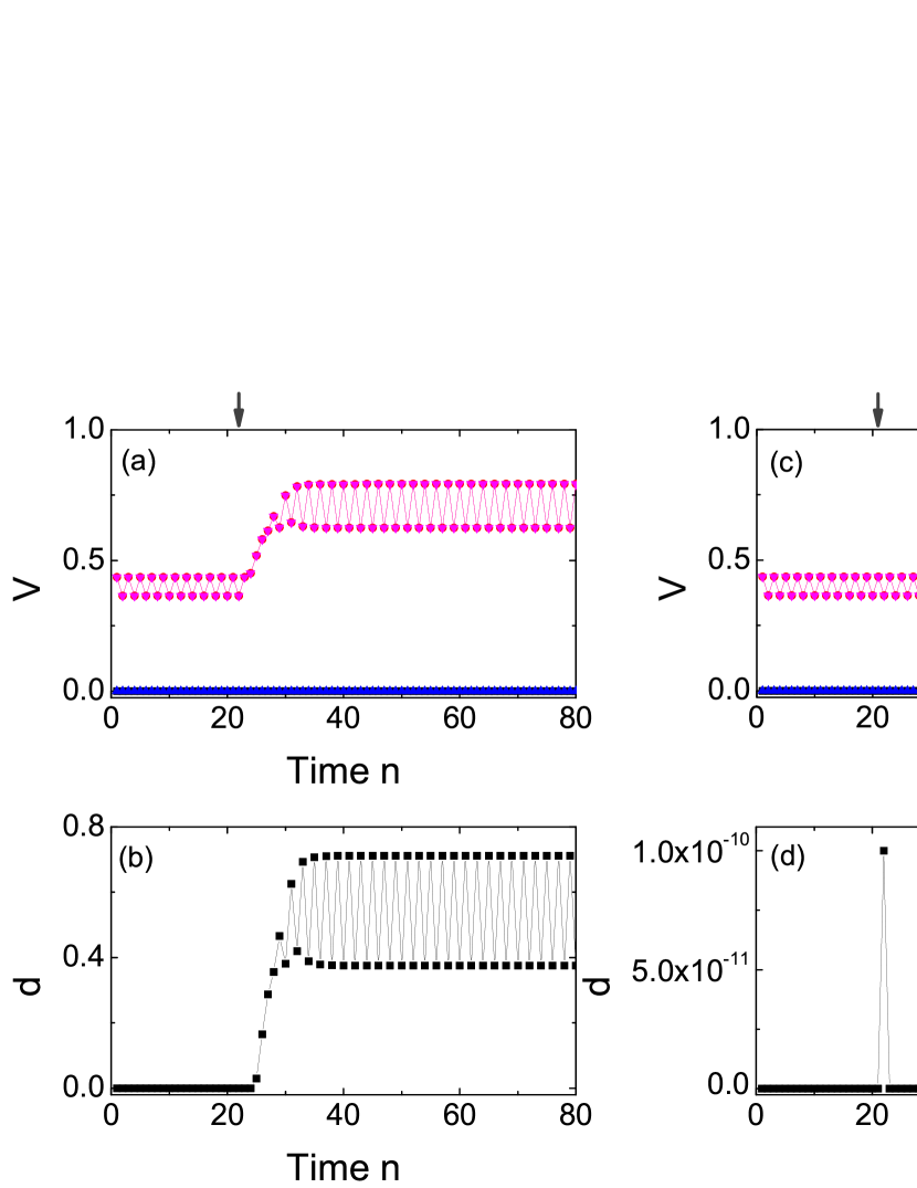
Figure 1: Responses of the instantaneous perturbation applied separately to an unstable and a stable point of a period-2 partially unstable attractor. Perturbation of strength $D=10^{-10}$ is applied at the position indicated by the arrow. In panels (a) and (c), the states $V$ of all oscillators versus the discrete time $n$ (corresponding to the $n$th reset of the reference oscillator 1) are shown. The state evolution of oscillators 1 and 3 is represented by the lower curve near zero, while the upper curve is for the evolution of oscillators 2 and 4. (a) Instantaneous perturbation on one point of the attractor can make the system approach a new attractor (see text for a detailed explanation). (b) The sequence of distance $d$ for the trajectory in (a) to the partially unstable attractor. (c) The stable response of the instantaneous perturbation on another point of the attractor. (d) The corresponding sequence of distance for the trajectory in (c) to the partially unstable attractor. The parameters of the system are $N=4$, $\tau=0.14$, $\varepsilon=0.3$, $B=1.6$, $I=3$, and $\omega=10$.

A simple example.

The simplest partially unstable attractor has period two, where one point is unstable and another is stable. Figure 1 shows an example of such an attractor in a system of $N=4$ globally coupled integrate-and-fire oscillators. After the system settles into this attractor, we let the system evolve without perturbation for $L$, say 10, periods (corresponding to $2L$ resets of the reference oscillator). We then introduce instantaneous perturbation separately to the states of oscillators just after $2L+1$ and those just after $2L+2$. Perturbation to the states of oscillators just after the 22nd (i.e., $L=10$) reset of reference oscillator 1 makes the system approach a new attractor, as shown in Fig. 1(a). This means that the corresponding point of the attractor is an unstable point. In order to show such process intuitively, we also measure the distance between the point on the perturbed trajectory to the original attractor. For example, the $i$th point on the perturbed trajectory is denoted by $P_{i}$. An attractor with period $m$ is represented by $m$ points, where each point is denoted as $Q_{i}$. The distance between point $P_{i}$ and the attractor is $d=\min_{j}\sum_{i}^{N}|P_{i}(k)-Q_{j}(k)|$. Here $P_{i}(k)$ and $Q_{j}(k)$ denote the state of oscillator $k$ for the $i$th point on the perturbed trajectory and the $j$th point on the attractor, respectively. The distance between the corresponding point on the perturbed trajectory and the original attractor, is shown in Fig. 1(b), where the distance finally becomes large, signifying the unstable nature of this point. The attractor, however, is stable with respect to perturbation on the other periodic point, as shown in Fig. 1(c), with the corresponding distance sequence displayed in Fig. 1(d). The system deviation from the periodic point due to the perturbation at the position of the arrow becomes zero after one reset of the reference oscillator, indicating the stable nature of the point. Physically, this is due to the passive firing on which the perturbation has little effect.

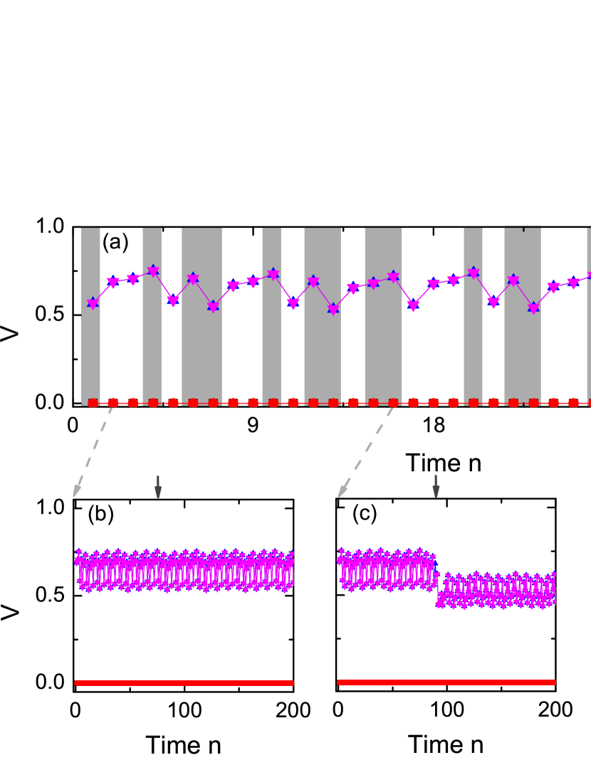
Figure 2: A partially unstable attractor of period 36. (a) Temporal evolution of all oscillators associated with a partially unstable attractor of period 36, where the unstable points are highlighted in gray, and the remaining points are stable. (b) The stable response of the system to perturbation applied at the position of the arrow. (c-d) Perturbation to the unstable point can make the system approach different attractors. Here time is represented by the $n$th reset of the reference oscillator 1, and the strength of the perturbation $D=10^{-12}$. System parameters are $N=4$, $\tau=0.2$, $\varepsilon=0.3$, $B=1.48$, $I=3$, and $\omega=10$.

A complex example.

For a partially unstable attractor with a period larger than two, the numbers of stable and unstable points can vary, and these two types of points can be mixed in a complicated way. Figure 2 shows a partially unstable attractor of period 36 in a system of $N=4$ globally coupled oscillators, where the unstable points are highlighted in gray (the remaining points are stable). The system state is robust against perturbation to the stable points, as shown in Fig. 2(b). However, perturbation to the unstable points can make the system transition to new attractors, as shown in Figs. 2(c,d).

To locate the partially unstable attractors with long periods can be extremely computationally demanding, as it is necessary to examine each point’s local dynamics. It has been known that periodic orbits of long periods are typical in the forced integrate-and-fire oscillators KHR:1981 , and even quasi-periodic attractors can emerge. Thus we focus on partially unstable attractors of period $2$ to address the issues of their existence and dynamical origin.

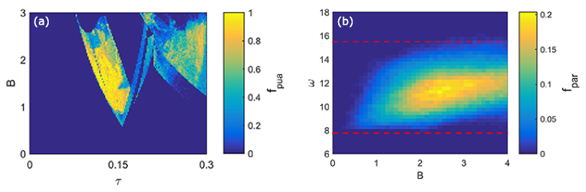
Figure 3: Parameter dependence of partially unstable attractors. For a system of $N=4$ oscillators, the dependence of the probability of partially unstable attractors of period two on parameters $\tau$ and $B$. (a) The fraction of initial conditions, $f_{pua}$, that lead to these attractors. The number of random initial conditions for each pair of parameters, $(\tau,B)$, is 200. (b) Dependence of $f_{par}$ on parameters $B$ and $\omega$, where $f_{par}$ is the relative size of the parameter region in $(\tau,\varepsilon)$ with period-2 partially unstable attractors. The two dashed lines indicate the estimated region for $\omega$. Other parameters are $\varepsilon=0.3$, $I=3$, and $\omega=10$. The strength $D$ of the perturbation is randomly chosen from the range [$10^{-13}$, $10^{-10}$].

4 Typicality and robustness of partially unstable attractors.

4.1 Partially unstable attractors under various parameters

We first identify the regions in the parameter plane ($\tau,B$) in which period-2 partially unstable attractors arise, for fixed $\omega=10$, $I=3$, $\varepsilon=0.3$, by calculating the fraction $f_{pua}$ of initial conditions that lead to these attractors. The $f_{pua}$ is obtained by using 200 random initial conditions. The results are shown in Fig. 3(a). We see that, in the parameter plane, the probability for generating period-2 partially unstable attractors is appreciable.

We next turn to the parameter $\omega$, the frequency of the applied current that defines an external time scale. An individual oscillator has its own time scale associated with its local dynamics, i.e., the time of free evolution from the reset to the next firing. It is useful to determine the relation between the two time scales, which can be done by analyzing the period of the free dynamics. Suppose that oscillator $i$ resets at $t_{a}$ with state $V_{i}^{a}=0$. The dynamics of free evolution can be obtained from Eq. 4 as

$$\begin{split}V_{i}(t)=&\frac{B\omega\sin{(\omega t)}+B\cos{(\omega t)}}{\omega^{2}+1}+\\ &I-e^{t_{a}-t}\{\frac{B\omega\sin{(\omega t_{a})}+B\cos{(\omega t_{a})}}{\omega^{2}+1}+I\}.\end{split}$$ (6)

The time duration $T_{d}$ before the threshold is reached again is $T_{d}=t-t_{a}$ for $V_{i}(t)=1$. The first term on the right-hand side of Eq. 6 can be written as

$$\frac{B\omega\sin{(\omega t)}+B\cos{(\omega t)}}{\omega^{2}+1}=\frac{B}{\sqrt{\omega^{2}+1}}\sin{(\omega t+\theta)},$$ (7)

where $\theta=\arctan{(1/\omega)}$. The maximum value of this term is about $B/\omega$. The effect of this term on $T_{d}$ can be neglected, if $B/\omega$ is much smaller than $I$, leading to $V_{i}(t)\approx I-e^{t_{a}-t}I$. We thus have

$$T_{d}\approx\log{(\frac{I}{I-1})}.$$ (8)

For the applied current with the frequency $\omega$, the time scale is $T_{\omega}=2\pi/\omega$. We can then investigate the interplay between $T_{d}$ and $T_{\omega}$ for period-2 partially unstable attractors, where each oscillator resets itself two times during $T_{\omega}$ time duration. Since $T_{d}$ only takes into account the free evolution and the arrival of pulses can increase the state value, we have $2T_{d}>T_{\omega}$. We can then estimate the maximum value of $T_{d}$. The partially unstable attractors typically emerge when the total coupling strength $\varepsilon$ is relatively small as compared with the threshold value. In this case, the value of $T_{d}$ should be smaller than $T_{\omega}$ so the states of oscillators can become close to the threshold. This way, oscillators can fire when receiving pulses during the time duration of $T_{\omega}$. The relation between $T_{d}$ and $T_{\omega}$ is thus $2T_{d}>T_{\omega}>T_{d}$ or

$$\pi/T_{d}<\omega<2\pi/T_{d}.$$ (9)

To demonstrate this result, we choose a large number of parameter points in the parameter plane $(B,\omega)$. For each point, we measure the relative size $f_{par}$ of the regions in another parameter plane, $(\tau,\varepsilon)$, in which partially unstable attractors arise. In the simulations, the ranges of $\tau$ and $\varepsilon$ are set to be $0.05\leqslant\tau\leqslant 0.5$ and $0.05\leqslant\varepsilon\leqslant 0.5$, respectively, which are covered by a $46\times 46$ grid, so we have $f_{par}\approx M_{pua}/(46\times 46)$, where $M_{pua}$ is the number of parameter points under which period-2 partially unstable attractors exist. For any given set of parameter values, we use $200$ random initial conditions in the phase space to determine whether there exists any period-2 partially unstable attractor. In particular, only when none of the 200 initial conditions leads to such an attractor do we deem that there is no partially unstable attractor for this parameter set. The quantity $f_{par}$ is essentially the probability of generating partially unstable attractors in the parameter plane $(\tau,\varepsilon)$ for any given values of $B$ and $\omega$. Figure 3(b) shows the dependence of $f_{par}$ on the parameters $(B,\omega)$, which gives direct evidence that period-2 partially unstable attractors exist in the region as predicted by Eq. 9, verifying the role of the interplay between the time scale of the individual oscillators and that of the external current in inducing such attractors.

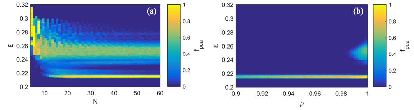
Figure 4: Existence of partially unstable attractors in globally coupled networks of various sizes and in non-globally coupled networks. (a) Dependence of $f_{pua}$ on the parameters $N$ and $\varepsilon$ for $\tau=0.14$, $I=3$, $\omega=10$, and $B=1.6$ in globally coupled systems. The non-zero value of $f_{pua}$ demonstrates that partially unstable attractors exist in systems of varying sizes. (b) Dependence of $f_{pua}$ on $\rho$, the density of links, and $\varepsilon$ for $N=60$, $\tau=0.14$, $I=3$, $\omega=10$, and $B=1.6$, which indicates that partially unstable attractors can exist for non-globally coupled networks of different values of the density of links. In both panels, $f_{pua}$ denotes the fraction of initial conditions that lead to partially unstable attractors of period 2.

4.2 Systems of different sizes and different coupling structures

Does the emergence of partially unstable attractors depend on the system size $N$? To address this question we examine the $(N,\varepsilon)$ parameter plane while fixing other parameters as $I=3$, $b=1.6$, $\omega=10,$ and $\tau=0.14$ (the latter four parameters are the same as in Fig. 1). For each parameter point in the parameter plane, we calculate the fraction $f_{pua}$ from an ensemble of 200 random initial conditions that lead to period-2 partially unstable attractors. Figure 4(a) shows the dependence of $f_{pua}$ on the system size $N$ and the normalized coupling strength $\varepsilon$. We see that the partially unstable attractors arise persistently in a wide range of the system size.

Would the coupling structure or network topology affect the occurrence of partially unstable attractors? For convenience, we use the density $\rho$ of directed links, defined as $\rho=m/[N(N-1)]$, to characterize the coupling structure of the network, where $N(N-1)$ is the number of links in a globally coupled network and $m<N(N-1)$ directed links are generated with each being placed between a pair of randomly selected oscillators. We focus on the parameter plane $(\rho,\varepsilon)$ and calculate, for each point in the plane, the fraction $f_{pua}$ of 200 random initial conditions that lead to partially unstable attractors. Ensemble average with 30 network realizations is used. Figure 4(b) shows $f_{pua}$ versus the density of links $\rho$ and the normalized coupling strength $\varepsilon$. Again, we find that partially unstable attractors are ubiquitous even when the network topology deviates from that of global coupling.

5 Dynamical origin of partially unstable attractors - event based analysis.

5.1 Symbolic events

There are two basic events associated with the dynamics of pulse-coupled integrate-and-fire networks: firing and receipt (arrival) of pulses. The events play a key role in understanding the collective dynamics such as the source of instability of unstable attractors zou:2010 and as well as the classification of multiple attractors zou:2012 . We exploit the two events to gain an understanding of the structure of partially unstable attractors in terms of the formation of the stable and unstable local dynamics.

Some basic notations for the events are as follows. When a pulse from oscillator $i$ is received by an oscillator in the network, this event is denoted as $R_{i}$. A pulse will be fired (or generated) when oscillator $j$ reaches its threshold, and this event is labeled as $S_{j}$. The events occurring at different times are separated by a minus sign. The firing events are of particular importance, where the firing may be due to the arrival of pulses immediately, or caused by the free dynamical evolution of the oscillator towards its threshold. In the former case, the event is called passive firing, where the arrival of pulses immediately makes the state value higher than the threshold. In the latter case, the firing occurs during the free evolution, and is thus termed active firing. The effect of instantaneous perturbation on the state of an actively firing oscillator is to cause a small change in the firing time. For example, the sequence of events labeled as “$R_{1}S_{2}-R_{2}-S_{3}$” denotes three events occurring at three different times. First, $R_{1}S_{2}$ represents the arrival of a pulse from oscillator 1, inducing the firing of oscillator 2. Hence $S_{2}$ is a passive firing event. Second, the pulse from oscillator 2 is received ($R_{2}$). Third, oscillator 3 reaches its threshold and fires: $S_{3}$ - an active firing event.

5.2 Event structure of a partially unstable attractor

How do partially unstable attractors arise and what are their event structures? For simplicity, we study the event structure associated with the period-2 partially unstable attractor presented in Fig. 1. The corresponding events are

$$R_{2}R_{4}-R_{1}R_{3}S_{2}S_{4}-R_{2}R_{4}S_{1}S_{3},\ \ \ \mbox{and}\ \ \ R_{1}R_{3}-S_{2}S_{4}-S_{1}S_{3}.$$ (10)

Each sequence of events corresponds to the events occurring during the time from the reset of the reference oscillator 1 to the next reset. One property of the event structure (10) is that multiple oscillators become simultaneously active firing or simultaneously passive firing at different times during one period, due to the role played by the alternating driving current. To demonstrate this, in the upper and lower panels of Fig. 5 we show respectively the time series of the applied current $I+B\cos(\omega t)$ and the states of the oscillators associated with the partially unstable attractor in Fig. 1. The states immediately after the events are shown in dots and triangles. The corresponding values of the alternating current are indicated by the vertical dashed lines.

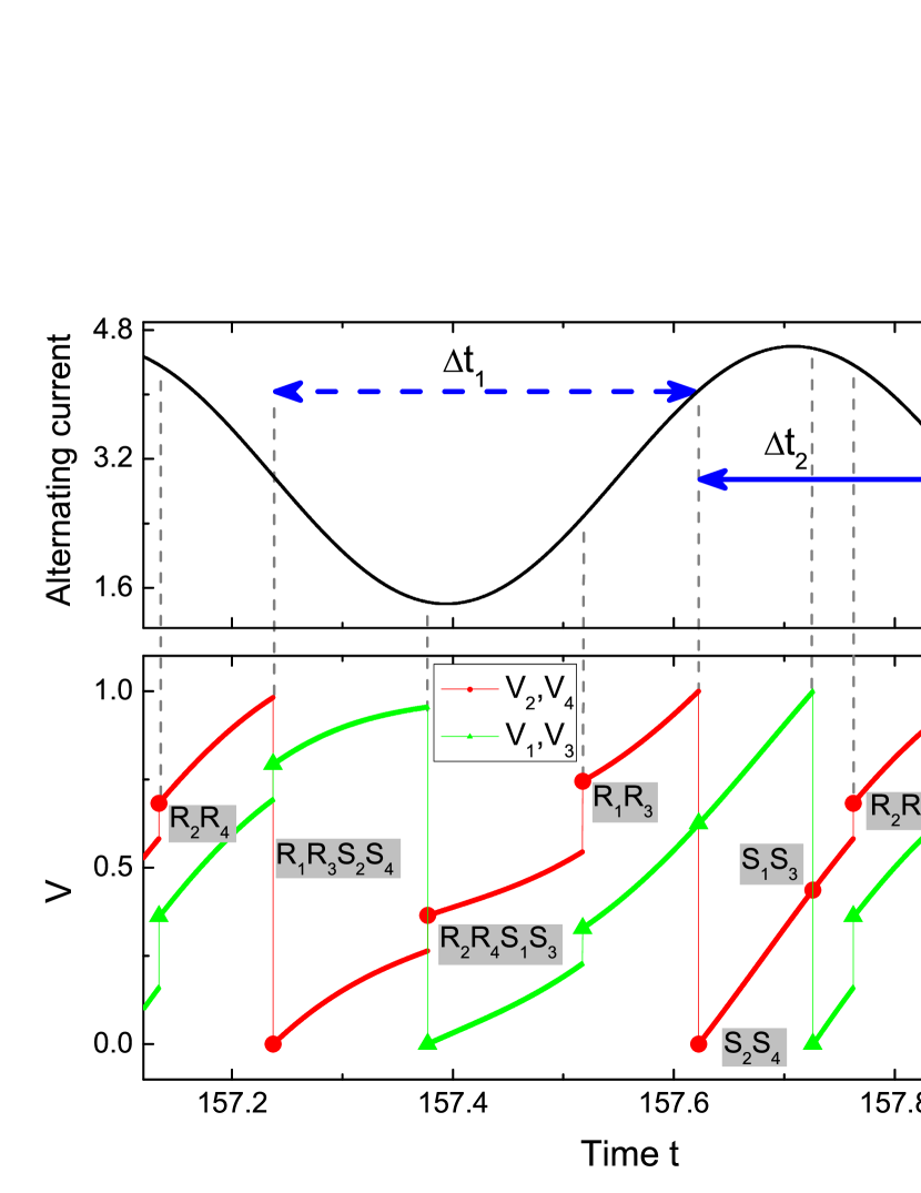
Figure 5: Event analysis of a period-2 partially unstable attractor. For $N=4$, $\tau=0.14$, $\varepsilon=0.3$, $B=1.6$, $I=3$, and $\omega=10$, the alternating current $I+B\cos(\omega t)$ (upper panel) and the state variable $V$ (lower panel) of all oscillators versus time $t$ associated with a partially unstable attractor. Oscillators 1 and 3 are synchronized, so are oscillators 2 and 4. The states immediately after every event are specified as red dots or green triangles. The corresponding values of the current are indicated by the vertical dashed lines.

To demonstrate the role of alternative current in shaping the structure (10), we first consider the time interval $\Delta t_{1}$ indicated in the upper panel of Fig. 5, where the event is from passive firing ($R_{1}R_{3}S_{2}S_{4}$) to active firing ($S_{2}S_{4}$). Oscillator 2 or 4 first receives a pulse after a time delay $\tau$ ($R_{2}R_{4}S_{1}S_{3}$) and then two pulses after another time delay $\tau$ ($R_{1}R_{3}$). During the time interval, the applied current is relatively small and thus contributes little to changing the state of oscillator 2 or 4. As a result, both oscillators 2 and 4 can generate active firing. Now consider the time duration $\Delta t_{2}$, where the event is from active firing $(S_{2}S_{4})$ to passive firing $(R_{1}R_{3}S_{2}S_{4})$. Oscillator 2 or 4 receives a pulse at time $\tau$ later $(R_{2}R_{4})$, and then two pulses at another time $t_{w}$ later $(R_{1}R_{3}S_{2}S_{4})$, where $t_{w}<\tau$. During $\Delta t_{2}$, the applied current is appreciable, so it drives the state of oscillator 2 or 4 to a large value, generating passive firing at the arrival of pulses from oscillators 1 and 3 $(R_{1}R_{3}S_{2}S_{4})$.

Table 1: A detailed description of events associated with the process that instantaneous perturbation is applied after the 22nd reset of the reference oscillator 1. The perturbation drives the system away from the attractor. Here time $n$ denotes the $n$th reset of the reference oscillator 1.

Time $n$	Events
18	$R_{2}R_{4}-R_{1}R_{3}S_{2}S_{4}-R_{2}R_{4}S_{1}S_{3}$
19	$R_{1}R_{3}-S_{2}S_{4}-S_{1}S_{3}$
20	$R_{2}R_{4}-R_{1}R_{3}S_{2}S_{4}-R_{2}R_{4}S_{1}S_{3}$
21	$R_{1}R_{3}-S_{2}S_{4}-S_{1}S_{3}$
22	$R_{2}R_{4}-R_{1}R_{3}S_{2}S_{4}-R_{2}R_{4}S_{1}S_{3}$
23	$R_{1}R_{3}-S_{4}-S_{2}-S_{3}-S_{1}$
24	$R_{4}-R_{2}-R_{3}S_{2}S_{4}-R_{1}-R_{2}R_{4}S_{1}S_{3}$
25	$R_{1}R_{3}-S_{2}S_{4}-S_{1}S_{3}$
26	$R_{2}R_{4}-S_{2}S_{4}-R_{1}R_{3}-R_{2}R_{4}S_{1}S_{3}$
27	$R_{1}R_{3}-S_{2}S_{4}-R_{2}R_{4}S_{1}S_{3}$
28	$S_{2}S_{4}-R_{1}R_{3}-R_{2}R_{4}S_{1}S_{3}$
29	$R_{1}R_{3}-S_{2}S_{4}-R_{2}R_{4}-S_{1}S_{3}$
30	$S_{2}S_{4}-R_{1}R_{3}-R_{2}R_{4}S_{1}S_{3}$

Intuitively, the effect of external driving on the state of each oscillator depends on time, due to the time varying nature of the driving current. In different time intervals, the rate of increase in the state value for each oscillator can then be different. A strong current can induce a large state change, which in turn can lead to passive firing, as the driving can push the corresponding oscillator towards the threshold. However, a weak current tends to give rise to active firings. An essential feature for partially unstable attractors is that multiple oscillators can become simultaneously active firing and simultaneously passive firing in different intervals during one period of the driving. As we demonstrate below, such an event structure is directly related to the coexistence of stable and unstable points on the attractor.

5.3 Understanding stable and unstable response

We then use the event structure to understanding the occurrence of the stable and the unstable point for the attractor shown in Fig. 1 with event structure (10). Under the return map, the attractor is composed of two points: $P$ and $Q$. Right after the first event sequence, the state of the system is $P$, while $Q$ is the state of the system immediately after the second event sequence. Here we let the system evolve for $L=10$ periods after the system settle into the attractor. Then points $Q$ and $P$ correspond to the states of oscillators at the 21st and 22nd reset of the reference oscillator respectively. The unstable and stable points are $P$ and $Q$, respectively, which can be established, as follows.

To ascertain that point $P$ is unstable, we apply perturbation to it, which is the state of the system right after the first sequence of events. Perturbation will affect the second sequence of events $R_{1}R_{3}-S_{2}S_{4}-S_{1}S_{3}$. In particular, due to the perturbation, the two simultaneously active firings $S_{2}S_{4}$ and $S_{1}S_{3}$ will be split into four single active firings. We find that the split of the event $S_{1}S_{3}$ is key to the emergence of the unstable local dynamics. Without perturbation, the pulses from oscillators 1 and 3 are received simultaneously and induce passive firing of oscillators 2 and 4 - hence the event $R_{1}R_{3}S_{2}S_{4}$. The states of oscillators 2 and 4 right before the $R_{1}R_{3}$ event are about 0.9821. Since the pulse strength is 0.1 and the threshold is 1, if $\delta_{3}>\delta_{1}$, oscillators 2 and 4 will receive one pulse first ($R_{3}$), which is sufficient to make them reach the threshold. The two oscillators then receive an extra pulse from oscillator 1 as compared with the case where there is no perturbation. This process can cause the system to transition to a remote state in the phase space. As a result, point $P$ is unstable. A detailed description of the events in response to the perturbation is provided in Table 1. Note that the split of $S_{2}S_{4}$ is not relevant, because the perturbation has little effect on oscillators 2 and 4 due to their passive firings $(R_{3}S_{2}S_{4})$ during the 24th reset of the reference oscillator, as shown in Table 1.

To determine that point $Q$ is stable, we apply instantaneous random perturbation ($\delta_{1},\delta_{2},\delta_{3},\delta_{4}$) to the states of the four oscillators, right after the reset of oscillator 1, and examine the effect of the perturbation on the first event sequence $R_{2}R_{4}-R_{1}R_{3}S_{2}S_{4}-R_{2}R_{4}S_{1}S_{3}$, where all four oscillators fire passively. For example, $R_{1}R_{3}S_{2}S_{4}$ denotes the event that oscillators 2 and 4 fire passively due to the arrival of pulses from oscillators 1 and 3. Immediately before the occurrence of this event, the states of oscillators 2 and 4 are slightly different due to the perturbation. Right after the event, the states of these two oscillators are reset to zero, effectively removing the effect of the perturbation. Similarly, the effect of $\delta_{1}$ and $\delta_{3}$ also disappears immediately after the $R_{2}R_{4}S_{1}S_{3}$ event. Due to the passive firings, point $Q$ is stable, i.e., the sequence of the arrival pulses for each oscillator will not be affected by perturbation applied to $Q$. Thus the perturbation in this case can not change the event structures.

Table 2: Examples of event structure for partially unstable attractors in a globally coupled oscillator system of size $N=60$. Other parameters are $\tau=0.14$, $I=3$, $\omega=10$, and $\varepsilon=0.25$. The oscillators with a synchronized state are regarded as belonging to one group. The number of groups determines the number of clusters in the phase space. The events of partially unstable attractors can be represented in terms of groups denoted as $A$, $B$, $C$, $D$, and so on. Five types of event structures are identified for the 238 period-2 partially unstable attractors obtained from 500 random initial conditions.

$i$th	Event
1	$R_{B}-R_{A}S_{B}-R_{B}S_{A}-R_{A}-S_{B}-S_{A}$
2	$R_{B}S_{C}-R_{A}S_{B}-R_{C}-R_{B}S_{A}-R_{A}-S_{C}-S_{B}-R_{C}-S_{A}$
3	$R_{B}-R_{A}-S_{D}-S_{C}-R_{D}S_{B}-S_{A}-R_{C}S_{D}-R_{B}-R_{A}S_{C}-R_{D}S_{B}-R_{C}S_{A}$
4	$R_{C}S_{D}-R_{B}S_{C}-R_{A}-R_{D}-R_{C}S_{B}-R_{B}S_{A}-S_{D}-S_{C}-R_{A}-R_{D}-S_{B}-S_{A}$
5	$R_{C}S_{D}-R_{B}-R_{A}S_{C}-S_{B}-R_{D}-R_{C}S_{A}-R_{B}-R_{A}-S_{D}-S_{C}-R_{D}S_{B}-S_{A}$

5.4 Event structure in larger systems.

We then study the event structures of period-2 partially unstable attractors in large globally coupled systems. The states of oscillators associated with an attractor in large systems are composed of multiple clusters, analogous to the partially unstable attractor with two clusters (Fig. 1) for a system of size $N=4$. Oscillators in each cluster have the same applied current and receive the same number of pulses at each arrival of pulses. The occurrence of the cluster structures is mainly due to the excitatory couplings. Suppose that some oscillators with states close to the threshold. At the arrival of some pulses at one time, these oscillators can reset, i.e., their states become zero, inducing one cluster for these oscillators. One can use such cluster structures to simplify the representation of the event structure for the whole system, where oscillators in the same cluster can be regarded as one group. In this way, the event structures for different systems may have similar structures, which can in turn be useful to understand the partially unstable attractors in large systems.

As a concrete example, we analyze the event structures for a system of $N=60$ globally coupled oscillators. Due to the symmetry of the system and its high dimensionality, a large number of period-2 partially unstable attractors can arise. In the representation based on groups, two distinct attractors can have the same event structure, if the corresponding groups of oscillators exhibit the same sequence of events. However individual oscillators for a group can be quite different, as the corresponding attractors are different. In this way, the types of event structures can be much fewer than the number of partially unstable attractors. For example, from 500 random initial conditions, we obtain 238 such attractors, but there are only 5 distinct types of event structure, as listed in Table 2.

For the first example in Table 2, the system has two clusters and the oscillators are organized into two groups: $A$ and $B$. Note that for different period-2 partially unstable attractors, group $A$ or $B$ has different oscillators. For example, for one such an attractor, group $A$ contains 27 oscillators (1, 3, 6, 7, 9, 12, 16, 17, 18, 25, 30, 31, 34, 37, 39, 40, 42, 46, 47, 48, 49, 50, 52, 53, 56, 59, and 60) and group $B$ contains all the remaining 33 oscillators. In terms of groups, we can compare the event structures of different partially unstable attractors, even for systems of different size. If, for the partially unstable attractor shown in Fig. 1 for $N=4$, we assign oscillators 2 and 4 as group $B$ and oscillators 1 and 3 as belonging to group $A$, the event structure in (10) is identical to that in the first example of Table 1. This implies that the occurrence of partially unstable attractors in large systems has the same dynamical mechanism as for smaller systems. This is indeed the case. We consider the event $R_{A}S_{B}$ here. The state of oscillators in group $B$ just before the arrival of pulses from oscillators of group $A$ ($R_{A}$) is 0.9645. With perturbations on the unstable point, the oscillators of group $A$ can become 27 single active firings at slightly different times. Here each pulse of strength $0.25/59$. The first 9 arrivals of pulses can make the group $B$ passive firing, i.e., $0.25/99\times 9+0.9645=1.0026>1$. Thus group $B$ will receive 18, i.e., 27-9, number of extra pulses, which can make the system leave away the unstable point. This mechanism is the same as that for the partially unstable attractor shown in Fig. 1.

6 Conclusion and discussion

Dissipative dynamical systems can exhibit different types of attractors. Attractors whose neighborhoods belong completely to their basins of attraction are the most commonly encountered type in smooth dynamical systems. When the system possesses certain simple symmetry so that there are invariant subspaces in which there are chaotic attractors, on any such attractor there can be a set of points that are unstable with respect to perturbation transverse to the invariant subspace. The number of points contained in such a set can be infinite but its measure is zero, and the corresponding attractors have a riddled basin - a type of Milnor attractors. Another type of Milnor attractors occurs typically in neuronal networks that exhibit a firing or spiking behavior, where the attractor is locally unstable but has a remote basin. Points in the basin are attracted towards the attractor along the stable manifold, but any random perturbation will “kick” the trajectory away from the attractor. These are the unstable attractors. The main contribution of this paper is the discovery and analysis of a novel type of attractors: partially unstable attractors. Such an attractor is composed of two subsets: one locally stable and another locally unstable, both of positive measures. We have demonstrated that partially unstable attractors can emerge in systems of excitatory pulse-coupled integrate-and-fire oscillators subject to periodic forcing. The mechanism for the partially unstable attractors can be understood by analyzing the dynamical events zou:2010 ; zou:2012 ; MT2006 leading to the generation of pulses in the network. In particular, the event of passive firing plays a key role in generating the locally stable set, where the effect of perturbation is suppressed and effectively annihilated. The locally unstable set arises due to the sensitivity of the number of arriving pulses for oscillators to perturbation.

Our results suggest that partially unstable attractors also persist on random networks. It is possible to study the existence of these attractors on other types of net- works, such as small-world networks, or networks with communities Newman:book . Insofar as the essential dynamical event structure can be identified, the possibility for partially unstable attractors to arise can be assessed. This can be useful for network design to achieve desired performance, e.g., for realizing specific firing sequences for information processing. For a given network whose structure cannot be altered, carefully controlling the periodic forcing may lead to desired firing patterns on the network level. To generate controlled dynamical behaviors in integrate-and-fire or more general neuronal networks remains to be an outstanding research task at the present.

In biological systems, information processing is often the result of interaction between the internal dynamical state and the external stimuli BUONOMANO:2009 . The uncovering and understanding of novel types of attractors in such systems can be beneficial MPJ:2012 . The existence of locally unstable dynamics can induce switchings among different metastable states, which can potentially be exploited for developing new schemes of computation RVLHAL:2001 ; AB:2005 ; NT:2012 ; HYZKY:2015 . In such an application, one wishes to generate switching dynamics that are robust to infinitesimal perturbation but sensitive to designed forcing. The switching dynamics among partially unstable attractors can be useful for achieving this goal. For example, infinitesimal perturbation can be directed to locally stable points, but forcing can be applied to locally unstable points. At the present, to exploit partially unstable attractors to generate robust yet sensitive switching dynamics is an open question.

References

References

- [1] E. Ott. Chaos in Dynamical Systems. Cambridge University Press, Cambridge, UK, second edition, 2002.
- [2] J.J. Hopfield. Neural networks and physical systems with emergent collective computational abilities. Proc. Nat. Acad. Sci. (USA), 79(8):2554–2558, 1982.
- [3] Y. Zhang, H. Zhang, and W. Gao. Multiple wada basins with common boundaries in nonlinear driven oscillators. Nonlinear Dynamics, 79(4):2667–2674, 2015.
- [4] Xiaojun Liu, Ling Hong, Jun Jiang, Dafeng Tang, and Lixin Yang. Global dynamics of fractional-order systems with an extended generalized cell mapping method. Nonlinear Dynamics, 83(3):1419–1428, 2016.
- [5] John Milnor. On the concept of attractor. In The Theory of Chaotic Attractors, pages 243–264. Springer, 2004.
- [6] Kunihiko Kaneko. Dominance of milnor attractors and noise-induced selection in a multiattractor system. Phys. Rev. Lett., 78(14):2736–2739, 1997.
- [7] J. C. Alexander, J. A. Yorke, Z. You, and I. Kan. Riddled basins. Int. J. Bifur. Chaos Appl. Sci. Eng., 2:795–813, 1992.
- [8] E. Ott, J. C. Sommerer, J. C. Alexander, I. Kan, and J. A. Yorke. Scaling behavior of chaotic systems with riddled basins. Phys. Rev. Lett., 71:4134–4137, 1993.
- [9] P. Ashwin, J. Buescu, and I. Stewart. Bubbling of attractors and synchronisation of oscillators. Phys. Lett. A, 193:126–139, 1994.
- [10] J. F. Heagy, T. L. Carroll, and L. M. Pecora. Experimental and numerical evidence for riddled basins in coupled chaotic systems. Phys. Rev. Lett., 73:3528–3531, 1994.
- [11] Y.-C. Lai, C. Grebogi, J. A. Yorke, and S. Venkataramani. Riddling bifurcation in chaotic dynamical systems. Phys. Rev. Lett., 77:55–58, 1996.
- [12] Y.-C. Lai and C. Grebogi. Noise-induced riddling in chaotic dynamical systems. Phys. Rev. Lett., 77:5047–5050, 1996.
- [13] H. Nakajima and Y. Ueda. Riddled basins of the optimal states in learning dynamical systems. Physica D, 99:35–44, 1996.
- [14] P. Ashwin, J. Buescu, and I. Stewart. From attractor to chaotic saddle: a tale of transverse instability. Nonlinearity, 9:703–737, 1996.
- [15] Y.-C. Lai. Scaling laws for noise-induced temporal riddling in chaotic systems. Phys. Rev. E, 56:3897–3908, 1997.
- [16] L. Billings, J. H. Curry, and E. Phipps. Lyapunov exponents, singularities, and a riddling bifurcation. Phys. Rev. Lett., 79:1018–1021, 1997.
- [17] Yu. Maistrenko, T. Kapitaniak, and P. Szuminski. Locally and globally riddled basins in two coupled piecewise-linear maps. Phys. Rev. E, 56:6393–6399, Dec 1997.
- [18] Y. L. Maistrenko, V. L. Maistrenko, A. Popovich, and E. Mosekilde. Transverse instability and riddled basins in a system of two coupled logistic maps. Phys. Rev. E, 57:2713–2724, 1998.
- [19] T. Kapitaniak, Y. Maistrenko, A. Stefanski, and J. Brindley. Bifurcation from locally to globally riddled basins. Phys. Rev. E, 58:8052–8052, 1998.
- [20] Y.-C. Lai and C. Grebogi. Riddling of chaotic sets in periodic windows. Phys. Rev. Lett., 83:2926–2929, 1999.
- [21] M. Woltering and M. Markus. Riddled-like basins of transient chaos. Phys. Rev. Lett., 84:630–633, 2000.
- [22] Y.-C. Lai and T. Tél. Transient Chaos: Complex Dynamics on Finite-Time Scales. Springer, New York, 2011.
- [23] Ligia Munteanu, Cornel Brişan, Veturia Chiroiu, Dan Dumitriu, and Rodica Ioan. Chaos–hyperchaos transition in a class of models governed by sommerfeld effect. Nonlinear Dynamics, 78(3):1877–1889, 2014.
- [24] Marc Timme, Fred Wolf, and Theo Geisel. Prevalence of unstable attractors in networks of pulse-coupled oscillators. Phys. Rev. Lett., 89(15):154105, 2002.
- [25] Marc Timme, Fred Wolf, and Theo Geisel. Unstable attractors induce perpetual synchronization and desynchronization. Chaos, 13(1):377–387, 2003.
- [26] Renato E Mirollo and Steven H Strogatz. Synchronization of pulse-coupled biological oscillators. SIAM J. Appl. Math., 50(6):1645–1662, 1990.
- [27] C. van Vreeswijk. Partial synchronization in populations of pulse-coupled oscillators. Phys. Rev. E, 54:5522–5537, Nov 1996.
- [28] Pulin Gong and Cees van Leeuwen. Dynamically maintained spike timing sequences in networks of pulse-coupled oscillators with delays. Phys. Rev. Lett., 98(4):048104, 2007.
- [29] Takashi Kanamaru and Kazuyuki Aihara. Roles of inhibitory neurons in rewiring-induced synchronization in pulse-coupled neural networks. Neural Comp., 22(5):1383–1398, 2010.
- [30] Stefano Luccioli and Antonio Politi. Irregular collective behavior of heterogeneous neural networks. Phys. Rev. Lett., 105(15):158104, 2010.
- [31] Stefano Luccioli, Simona Olmi, Antonio Politi, and Alessandro Torcini. Collective dynamics in sparse networks. Phys. Rev. Lett., 109(13):138103, 2012.
- [32] Alexander Zumdieck, Marc Timme, Theo Geisel, and Fred Wolf. Long chaotic transients in complex networks. Phys. Rev. Lett., 93(24):244103, 2004.
- [33] Rüdiger Zillmer, Roberto Livi, Antonio Politi, and Alessandro Torcini. Desynchronization in diluted neural networks. Phys. Rev. E, 74(3):036203, 2006.
- [34] Sven Jahnke, Raoul-Martin Memmesheimer, and Marc Timme. Stable irregular dynamics in complex neural networks. Phys. Rev. Lett., 100(4):048102, 2008.
- [35] Christoph Kirst and Marc Timme. How precise is the timing of action potentials? Front. Neurosci., 3(1):2–3, 2009.
- [36] Rüdiger Zillmer, Nicolas Brunel, and David Hansel. Very long transients, irregular firing, and chaotic dynamics in networks of randomly connected inhibitory integrate-and-fire neurons. Phys. Rev. E, 79(3):031909, 2009.
- [37] Hailin Zou, Shuguang Guan, and C-H Lai. Dynamical formation of stable irregular transients in discontinuous map systems. Phys. Rev. E, 80(4):046214, 2009.
- [38] A Rothkegel and K Lehnertz. Irregular macroscopic dynamics due to chimera states in small-world networks of pulse-coupled oscillators. New J. Phys., 16(5):055006, 2014.
- [39] Marc Timme, Fred Wolf, and Theo Geisel. Coexistence of regular and irregular dynamics in complex networks of pulse-coupled oscillators. Phys. Rev. Lett., 89(25):258701, 2002.
- [40] Antonio Politi and Stefano Luccioli. Dynamics of networks of leaky-integrate-and-fire neurons. In Net. Sci., pages 217–242. Springer, 2010.
- [41] Simona Olmi, Alessandro Torcini, and Antonio Politi. Linear stability in networks of pulse-coupled neurons. Front. Comp. Neurosci., 8:00008, 2014.
- [42] Antonio Politi and Michael Rosenblum. Equivalence of phase-oscillator and integrate-and-fire models. Phys. Rev. E, 91(4):042916, 2015.
- [43] Hailin Zou, Xiaofeng Gong, and C-H Lai. Unstable attractors with active simultaneous firing in pulse-coupled oscillators. Phys. Rev. E, 82(4):046209, 2010.
- [44] Peter Ashwin and Marc Timme. Unstable attractors: existence and robustness in networks of oscillators with delayed pulse coupling. Nonlinearity, 18(5):2035–2060, 2005.
- [45] Henk Broer, Konstantinos Efstathiou, and Easwar Subramanian. Robustness of unstable attractors in arbitrarily sized pulse-coupled networks with delay. Nonlinearity, 21(1):13–49, 2008.
- [46] Henk Broer, Konstantinos Efstathiou, and Easwar Subramanian. Heteroclinic cycles between unstable attractors. Nonlinearity, 21(6):1385–1410, 2008.
- [47] Christoph Kirst and Marc Timme. From networks of unstable attractors to heteroclinic switching. Phys. Rev. E, 78(6):065201, 2008.
- [48] Christoph Kirst, Theo Geisel, and Marc Timme. Sequential desynchronization in networks of spiking neurons with partial reset. Phys. Rev. Lett., 102(6):068101, 2009.
- [49] Fabio Schittler Neves and Marc Timme. Computation by switching in complex networks of states. Phys. Rev. Lett., 109(1):018701, 2012.
- [50] Fabio Schittler Neves and Marc Timme. Controlled perturbation-induced switching in pulse-coupled oscillator networks. J. Phys. A Math. Theo., 42(34):345103, 2009.
- [51] G Manjunath, P Tino, and H Jaeger. Theory of input driven dynamical systems. Dice. Ucl. Ac. Be., pages 25–27, 2012.
- [52] James P Keener, FC Hoppensteadt, and J Rinzel. Integrate-and-fire models of nerve membrane response to oscillatory input. SIAM J. Appl. Math., 41(3):503–517, 1981.
- [53] Hai-Lin Zou, Menghui Li, Choy-Heng Lai, and Ying-Cheng Lai. Origin of chaotic transients in excitatory pulse-coupled networks. Phys. Rev. E, 86(6):066214, 2012.
- [54] Raoul-Martin Memmesheimer and Marc Timme. Designing the dynamics of spiking neural networks. Phys. Rev. Lett., 97(18):188101, 2006.
- [55] M. E. J. Newman. Networks: An Introduction. Oxford University Press, Oxford, first edition, 2010.
- [56] D.V. Buonomano and W. Maass. State-dependent computations: spatiotemporal processing in cortical networks. Nat. Rev. Neurosci., 10(2):113–125, 2009.
- [57] M Rabinovich, A Volkovskii, P Lecanda, R Huerta, HDI Abarbanel, and G Laurent. Dynamical encoding by networks of competing neuron groups: winnerless competition. Phys. Rev. Lett., 87(6):068102, 2001.
- [58] Peter Ashwin and Jon Borresen. Discrete computation using a perturbed heteroclinic network. Phys. Lett. A, 347(4):208–214, 2005.
- [59] H.-L. Zou, Y. Katori, Z.-C. Deng, K. Aihara, and Y.-C. Lai. Controlled generation of switching dynamics among metastable states in pulse-coupled oscillator networks. Chaos, 25(10):103109, 2015.