Equality in Borell-Brascamp-Lieb inequalities on curved spaces

Abstract.

By using optimal mass transportation and a quantitative Hölder inequality, we provide estimates for the Borell-Brascamp-Lieb deficit on complete Riemannian manifolds. Accordingly, equality cases in Borell-Brascamp-Lieb inequalities (including Brunn-Minkowski and Prékopa-Leindler inequalities) are characterized in terms of the optimal transport map between suitable marginal probability measures. These results provide several qualitative applications both in the flat and non-flat frameworks. In particular, by using Caffarelli’s regularity result for the Monge-Ampère equation, we give a new proof of Dubuc’s characterization of the equality in Borell-Brascamp-Lieb inequalities in the Euclidean setting. When the $n$-dimensional Riemannian manifold has Ricci curvature ${\rm Ric}(M)\geq(n-1)k$ for some $k\in\mathbb{R}$, it turns out that equality in the Borell-Brascamp-Lieb inequality is expected only when a particular region of the manifold between the marginal supports has constant sectional curvature $k$. A precise characterization is provided for the equality in the Lott-Sturm-Villani-type distorted Brunn-Minkowski inequality on Riemannian manifolds. Related results for (not necessarily reversible) Finsler manifolds are also presented.

Dedicated to our friend, Professor Csaba Varga.

Keywords: Borell-Brascamp-Lieb inequality; Brunn-Minkowski inequality; Prékopa-Leindler inequality; equality case; optimal mass transportation; Riemannian manifold; Finsler manifold.

MSC: 49Q20; 53C21; 39B62; 53C24; 58E35.

1. Introduction

1.1. Background and motivation

The Borell-Brascamp-Lieb inequality in the Euclidean space $\mathbb{R}^{n}$ states that for every fixed $s\in(0,1)$, $p\geq-\frac{1}{n}$ and integrable functions $f,g,h:\mathbb{R}^{n}\to[0,\infty)$ which satisfy

$$h((1-s)x+sy)\geq\mathcal{M}_{s}^{p}\left(f(x),g(y)\right)\quad\mbox{ for all }x,y\in\mathbb{R}^{n},$$ (1.1)

one has

$$\int_{\mathbb{R}^{n}}h\geq\mathcal{M}_{s}^{\frac{p}{1+np}}\left(\int_{\mathbb{R}^{n}}f,\int_{\mathbb{R}^{n}}g\right).$$ (1.2)

Here, for every $s\in(0,1)$, $p\in\mathbb{R}\cup\{\pm\infty\}$ and $a,b\geq 0$, the $p$-mean is defined by

$$\mathcal{M}_{s}^{p}(a,b)=\left\{\begin{array}[]{lll}\left((1-s)a^{p}+sb^{p}\right)^{1/p}&\mbox{if}&ab\neq 0,\\ 0&\mbox{if}&ab=0,\end{array}\right.$$

with the conventions $\mathcal{M}_{s}^{-\infty}(a,b)=\min\{a,b\}$; $\mathcal{M}_{s}^{0}(a,b)=a^{1-s}b^{s};$ and $\mathcal{M}_{s}^{+\infty}(a,b)=\max\{a,b\}$ if $ab\neq 0$ and $\mathcal{M}_{s}^{+\infty}(a,b)=0$ if $ab=0$.

In terms of entropy, Borell-Brascamp-Lieb inequality implies that if a Radon measure $\mu$, has as density $\rho$ a $p$-concave function (i.e., $f=g=h=\rho$ satisfies (1.1)), then $\mu$ is a $q$-concave measure with the parameter $q=\frac{p}{1+np}\in[-\infty,\frac{1}{n}]$. A sort of converse of the latter statement is given by Borell [8], characterizing the $q$-concave measures by means of $p$-concave functions. Further contributions to this subject can be found in Bobkov and Ledoux [6], Brascamp and Lieb [10]. In particular, $0$-concave measures are characterized by log-concave density functions, while $\frac{1}{n}$-concave measures on convex sets are equal to the Lebesgue $\mathcal{L}^{n}$-measure up to a multiplicative constant.

Another important consequence of the Borell-Brascamp-Lieb inequality (for $p=+\infty$ and indicator functions) is the usual Brunn-Minkowski inequality, implying e.g. the isoperimetric inequality, which relates the $\mathcal{L}^{n}$-measure of two measurable sets $A$ and $B$ in $\mathbb{R}^{n}$ with the (outer) $\mathcal{L}^{n}$-measure of their Minkowski sum $(1-s)A+sB=\{(1-s)x+sy:x\in A,y\in B\}$ as

$$\mathcal{L}^{n}((1-s)A+sB)^{\frac{1}{n}}\geq(1-s)\mathcal{L}^{n}(A)^{\frac{1}{n}}+s\mathcal{L}^{n}(B)^{\frac{1}{n}}.$$ (1.3)

An equivalent form of (1.3), coming also from the Borell-Brascamp-Lieb inequality (for $p=0$ and indicator functions), is the dimension-free-Brunn-Minkowski inequality, – or the geometric form of the Prékopa-Leindler inequality, – which states that

$$\mathcal{L}^{n}((1-s)A+sB)\geq\mathcal{L}^{n}(A)^{1-s}\mathcal{L}^{n}(B)^{s}.$$ (1.4)

Characterizations of cases of equality and the problem of stability in the aforementioned inequalities (1.2)-(1.4) are still subjects for further investigation. After the pioneering works by Brunn and Minkowski, it is well known for more than a century that equality in (1.3) holds if and only if the sets $A$ and $B$ are homothetic convex bodies from which sets of measure zero have been removed; similarly, equality in (1.4) holds if and only if the sets $A$ and $B$ are translated convex bodies up to a null measure set. The equality case in the generic Borell-Brascamp-Lieb inequality (1.2) has been studied in the mid of seventies by Dubuc [21] on $\mathbb{R}^{n}$ by using deep convexity and measure theoretical results together with a careful inductive argument w.r.t. the dimension of the space $\mathbb{R}^{n}$. Later on, Dancs and Uhrin [18, 19] obtained some qualitative Borell-Brascamp-Lieb inequalities on $\mathbb{R}$, providing also some higher-dimensional versions. A few years ago, Ball and Böröczky [2, 3] obtained stability results for the one-dimensional functional Prékopa-Leindler inequality with some extensions also to higher-dimensions. Very recently, various stability results are established in $\mathbb{R}^{n}$ for the generic Borell-Brascamp-Lieb inequality by Ghilli and Salani [28], Rossi [41], Rossi and Salani [42, 43], for the Prékopa-Leindler inequality by Bucur and Fragalà [11], and for the Brunn-Minkowski inequality by Christ [13], Figalli and Jerison [23, 22, 24] and Figalli, Maggi and Pratelli [25, 26]. The common strategy in the aforementioned papers, up to the latter two papers, is the use of various arguments from convex analysis combined usually with some inductive step w.r.t. the dimension, by fully exploring the Euclidean character of the space. In [25, 26], quantitative Brunn-Minkowski inequalities are established by using optimal mass transportation arguments in $\mathbb{R}^{n}.$ Further results concerning equality and stability in the Brunn-Minkowski inequality in $\mathbb{R}^{n}$ can be found in Milman and Rotem [36] and Colesanti, Livshyts and Marsiglietti [15].

As far as we know, no equality/stability results are available for Borell-Brascamp-Lieb inequalities on curved spaces. It is clear that the arguments from the aforementioned papers (see [2], [3], [11], [13], [18], [21], [22], [23], and references therein) cannot be applied in such a nonlinear setting. The starting point of our investigation is the celebrated work by Cordero-Erausquin, McCann and Schmuckenschläger [17] who established a Riemannian version of the Borell-Brascamp-Lieb inequality via optimal mass transportation culminating in a distorted Jacobian determinant inequality. The Finslerian counterparts of the results from [17] are provided by Ohta [38]. We point out that the first optimal mass transportation approaches to geometric inequalities have been provided by Gromov in [37] (via the Knothe map) and McCann [34], [35, Appendix D] (via the Brenier map). It is worth mentioning that Knothe [29] himself used his map to prove the generalized Brunn-Minkowski inequality (1.4).

The main purpose of our paper is to characterize the equality in Borell-Brascamp-Lieb inequalities on complete $n$-dimensional Riemannian/Finsler manifolds for the whole spectrum of the parameter $p\geq-\frac{1}{n}$ by exploring a quantitative Hölder inequality and the theory of optimal mass transportation.

In the sequel, we roughly present some of our achievements.

1.2. Brief description of main results and consequences

Let $(M,w)$ be a complete $n$-dimensional Riemannian manifold $(n\geq 2)$ with the induced distance function $d:M\times M\to[0,\infty)$; without mentioning explicitly, we assume throughout the whole paper that $(M,w)$ is connected. For a fixed $s\in(0,1)$ and $(x,y)\in M\times M$ let

$$Z_{s}(x,y)=\{z\in M:d(x,z)=sd(x,y),\ d(z,y)=(1-s)d(x,y)\}$$

be the set of $s$-intermediate points between $x$ and $y$, replacing the convex combination in (1.1). Since $(M,d)$ is complete, $Z_{s}(x,y)\neq\emptyset$ for every $x,y\in M.$ Accordingly, the Minkowski interpolation set

$$Z_{s}(A,B)=\bigcup\limits_{(x,y)\in A\times B}Z_{s}(x,y)$$

replaces the Minkowski sum of the nonempty sets $A,B\subset M$.

Let $s\in(0,1)$ and $p\geq-\frac{1}{n}$. If $f,g,h:M\to[0,\infty)$ are three nonzero, compactly supported integrable functions, the natural Riemannian reformulation of (1.1) reads as

$$h(z)\geq\mathcal{M}^{p}_{s}\left(\frac{f(x)}{v_{1-s}(y,x)},\frac{g(y)}{v_{s}(x,y)}\right)\ \ {\rm for\ all}\ (x,y)\in M\times M,z\in Z_{s}(x,y),$$ (1.5)

where $v_{s}$ is the volume distortion coefficient (see (2.3) for its precise definition). Under the assumption (1.5), the main result of Cordero-Erausquin, McCann and Schmuckenschläger [17] says that

$$\int_{M}h\geq\mathcal{M}_{s}^{\frac{p}{1+np}}\left(\int_{M}f,\int_{M}g\right),$$ (1.6)

where the integrals are considered w.r.t. the Riemannian measure m on $(M,w)$. This will be referred throughout the paper as the Borell-Brascamp-Lieb inequality with exponent $p$.

For simplicity of notation, let $\|\cdot\|_{1}$ be the $L^{1}$-norm of any integrable function on $M.$ For the above functions $f,g$ and $h$, let us consider the Borell-Brascamp-Lieb deficit given by

$$\delta_{M,s}^{p}(f,g,h)=\frac{\|h\|_{1}}{\mathcal{M}_{s}^{\frac{p}{1+pn}}\left(\|f\|_{1},\|g\|_{1}\right)}-1.$$

We first provide an estimate for the Borell-Brascamp-Lieb deficit on a general Riemannian manifold that will be achieved by using optimal mass transportation and a quantitative Hölder inequality:

Theorem 1.1.

(Estimate of the Borell-Brascamp-Lieb deficit) Let $(M,w)$ be a complete $n$-dimensional Riemannian manifold, $s\in(0,1),$ $p\geq-\frac{1}{n}$ and $f,g,h:M\to[0,\infty)$ be three nonzero, compactly supported integrable functions satisfying $(\ref{ConditionRescaledBBLWithWeights-vege}).$ Then

$$\delta_{M,s}^{p}(f,g,h)\geq\displaystyle\int_{M}\tilde{f}(x)G_{s}^{p,n}\left(\frac{f(x)}{v_{1-s}(\psi(x),x)},\frac{g(\psi(x))}{v_{s}(x,\psi(x))},\frac{1}{\|f\|_{1}},\frac{1}{\|g\|_{1}}\right){\rm d}\sf{m},$$

where $\psi:M\to M$ is the unique optimal transport map from the measure $\mu=\tilde{f}{\rm d}\sf{m}$ to $\nu=\tilde{g}{\rm d}\sf{m}$ with densities $\tilde{f}=f/\|f\|_{1}$, $\tilde{g}=g/\|g\|_{1}$, and $G_{s}^{p,n}\geq 0$ is the gap-function given in Lemma $\ref{lemma-p-mean}.$

The uniqueness of the optimal transport map $\psi:M\to M$ from the probability measure $\mu=\tilde{f}{\rm d}\textsf{m}$ to $\nu=\tilde{g}{\rm d}\textsf{m}$ is well known by McCann [33] having the form $\psi(x)=\exp_{x}(-\nabla\varphi(x))$ for a.e. $x\in\operatorname{supp}f$ for some $d^{2}/2$-concave function $\varphi:M\to\mathbb{R},$ where $\nabla$ denotes the Riemannian gradient. Let $\psi_{s}:M\to M$ be the $s$-interpolant optimal transport map $\psi_{s}(x)=\exp_{x}(-s\nabla\varphi(x))$ for a.e. $x\in\operatorname{supp}f$, and Jac$(\psi_{s})(x)$ its Jacobian in a.e. $x\in\operatorname{supp}f$.

By Theorem 1.1 the equality in the Borell-Brascamp-Lieb inequality can be characterized by studying the properties of the gap-function $G_{s}^{p,n},$ leading us to the following result:

Theorem 1.2.

(Equality in Borell-Brascamp-Lieb inequality; $p>-\frac{1}{n}$) Let $(M,w)$ be a complete $n$-dimensional Riemannian manifold, $s\in(0,1),$ $p>-\frac{1}{n}$ and $f,g,h:M\to[0,\infty)$ be three nonzero, compactly supported integrable functions satisfying $(\ref{ConditionRescaledBBLWithWeights-vege}).$ Then the following two assertions are equivalent:

• $\delta_{M,s}^{p}(f,g,h)=0,$ i.e., equality holds in the Borell-Brascamp-Lieb inequality;

• the following statements simultaneously hold$:$

  • $\operatorname{supp}h=\psi_{s}(\operatorname{supp}f)$ up to a null measure set;

  • ${\rm Jac}(\psi_{s})(x)={v_{1-s}(\psi(x),x)}\left[\mathcal{M}_{s}^{\frac{p}{pn+1}}\left(1,\frac{\|g\|_{1}}{\|f\|_{1}}\right)\right]^{\frac{pn}{pn+1}}$ for a.e. $x\in\operatorname{supp}f;$

  • for a.e. $x\in\operatorname{supp}f$, one has

    $$\frac{h(\psi_{s}(x))}{\left[\mathcal{M}_{s}^{\frac{p}{pn+1}}(\|f\|_{1},\|g\|_{1})\right]^{\frac{1}{pn+1}}}=\frac{f(x)}{v_{1-s}(\psi(x),x)\|f\|_{1}^{\frac{1}{pn+1}}}=\frac{g(\psi(x))}{v_{s}(x,\psi(x))\|g\|_{1}^{\frac{1}{pn+1}}}.$$

The equality in the Borell-Brascamp-Lieb inequality for $p=-\frac{1}{n}$ is genuinely different than the case $p>-\frac{1}{n}$ and it will be treated separately in Theorem 2.1.

Theorem 1.2 provides both well known and genuinely new rigidity results; we briefly present some of them in the sequel (for details, see §3 and §4):

$\bullet$ Equality in the Borell-Brascamp-Lieb inequality in $\mathbb{R}^{n}$: a new approach to Dubuc’s characterization. As a first consequence of Theorem 1.2 we prove that equality in the Borell-Brascamp-Lieb inequality in $\mathbb{R}^{n}$ holds if and only if the functions $f,$ $g$ and $h$ are obtained as compositions of fixed $(t,p)$-concave function $\Phi$ with appropriate homotheties, where the support of $\Phi$ is convex up to a null set; for the precise statement, see Theorem 3.1. This result provides a new qualitative formulation of Dubuc’s characterization, see [21, Théorème 12]. Our strategy relies on applying Theorem 1.2 in order to reduce the problem to the equality case in the Brunn-Minkowski inequality for the marginal supports $\operatorname{supp}f$ and $\operatorname{supp}g$, implying the convexity of these sets. Using the convexity of the support of the target measure, a suitable application of the celebrated regularity result of Caffarelli [12] provides smoothness of the optimal mass transport map which turns to be an affine function in $\mathbb{R}^{n}$. We notice that Caffarelli’s regularity has been already employed in order to establish sharp stability results in $\mathbb{R}^{n}$ for the Brunn-Minkowski inequality (1.3), see Figalli, Maggi and Pratelli [25, 26].

$\bullet$ Equality in Borell-Brascamp-Lieb inequality implies constant curvature. We state that the equality in the Borell-Brascamp-Lieb inequality on an $n$-dimensional Riemannian manifold with Ricci curvature Ric$(M)\geq k(n-1)$ for some $k\in\mathbb{R}$ can be expected to hold only when a particular region of the manifold between the marginal supports has constant sectional curvature $k$; see Theorem 4.1 for details. The proof is based on Theorem 1.2 and a careful comparison argument à la Bishop-Crittenden of the volume distortion coefficients with suitable quantities involving Jacobi fields on space forms.

$\bullet$ Equality in distorted Brunn-Minkowski inequality à la Lott-Sturm-Villani. For some $s\in(0,1)$, $k\in\mathbb{R}$ and $n\geq 2$, let

$$\tau_{s}^{k,n}(\theta)=\left\{\begin{array}[]{lll}s^{\frac{1}{n}}\left(\sinh\left(\sqrt{-k}s\theta\right)\big{/}\sinh\left(\sqrt{-k}\theta\right)\right)^{1-\frac{1}{n}}&{\rm if}&k\theta^{2}<0;\\ s&{\rm if}&k\theta^{2}=0;\\ s^{\frac{1}{n}}\left(\sin\left(\sqrt{k}s\theta\right)\big{/}\sin\left(\sqrt{k}\theta\right)\right)^{1-\frac{1}{n}}&{\rm if}&0<k\theta^{2}<\pi^{2};\\ +\infty&{\rm if}&k\theta^{2}\geq\pi^{2},\end{array}\right.$$

be the distortion coefficient introduced independently by Lott and Villani [31] and Sturm [47] in order to define their famous curvature-dimension condition $\textsf{CD}(k,n)$ on metric measure spaces. Let $(M,w)$ be a complete $n$-dimensional Riemannian manifold with Ricci curvature bounded below, i.e., Ric$(M)\geq k(n-1)$ for some $k\in\mathbb{R}$ (which is equivalent to the validity of $\textsf{CD}(k,n)$) and let us denote by m the Riemannian measure on $M$. The distorted Brunn-Minkowski inequality reads as

$$\textsf{m}(Z_{s}(A,B))^{\frac{1}{n}}\geq\tau_{1-s}^{k,n}(\Theta_{A,B})\textsf{m}(A)^{\frac{1}{n}}+\tau_{s}^{k,n}(\Theta_{A,B})\textsf{m}(B)^{\frac{1}{n}},$$ (1.7)

where $A,B\subset M$ are measurable sets with $\textsf{m}(A)\neq 0\neq\textsf{m}(B)$ and

$$\Theta_{A,B}=\left\{\begin{array}[]{lll}\inf_{(x,y)\in A\times B}d(x,y)&\mbox{if}&k\geq 0;\\ \sup_{(x,y)\in A\times B}d(x,y)&\mbox{if}&k<0,\end{array}\right.$$ (1.10)

see Sturm [47, Proposition 2.1] and Villani [48, Theorem 18.5]. Hereafter, the measure of $Z_{s}(A,B)$ in (1.7) is always understood w.r.t. the outer measure $\textsf{m}^{*}$ of $\textsf{m}.$ In fact, inequality (1.7) is a direct consequence of the Borell-Brascamp-Lieb inequality (1.6) even on metric measure spaces verifying the $\textsf{CD}(k,n)$ condition, see Bacher [1, Proposition 3.2]; we also recall its proof in subsection 4.2. Theorem 1.2 provides the following scenario concerning the equality in (1.7) (for details, see Theorem 4.2):

1. Positively curved case: if $k>0$ (e.g., the round sphere $\mathbb{S}^{n}$), then equality in (1.7) is characterized by the overlapping of the sets $Z_{s}(A,B)$, $A$ and $B$ up to a null measure set. Moreover, if $A\times B$ does not contain cut locus pairs, equality holds in (1.7) if and only if there exists an open, geodesic convex set in $M$ which differs from $A$ and $B$ by a null set.

2. Negatively curved case: if $k<0$ and $(M,g)$ has nonpositive, nonzero sectional curvature (e.g., the hyperbolic space $\mathbb{H}^{n}$), equality in (1.7) cannot hold for any positive measure sets $A$ and $B$.

The proof of the latter statements are based on a porosity argument and a geometric form of the Steinhaus density theorem (concerning the ’difference’ of two sets).

1.3. Organization of the paper

In §2 we first state a quantitative Hölder inequality (see Lemma 2.1) which is crucial in the proof of Theorem 1.1. We then prove simultaneously Theorems 1.1 and 1.2. In §3 we prove Theorem 3.1 which provides a qualitative version of Dubuc’s characterization in $\mathbb{R}^{n}$ concerning the equality case in the Borell-Brascamp-Lieb inequality. In §4 we deal with Riemannian manifolds by proving that the equality in Borell-Brescamp-Lieb inequality implies constant curvature, see Theorem 4.1, and we discuss the equality cases in the distorted Brunn-Minkowski inequality (1.7), see Theorem 4.2. In §5 certain Borell-Brascamp-Lieb inequalities are presented on not necessarily reversible Finsler manifolds, highlighting some subtle differences between Riemannian/Euclidean and Finslerian frameworks, respectively, (see e.g. Corollary 5.2). Finally, in §6, we provide the proof of Lemma 2.1.

2. A quantitative Hölder inequality and the Borell-Brascamp-Lieb deficit: proof of main results

It is known (see e.g. Gardner [27, Lemma 10.1]) the following version of the Hölder inequality

$$\mathcal{M}_{s}^{p}(a,b)\mathcal{M}_{s}^{q}(c,d)\geq\mathcal{M}_{s}^{\eta}(ac,bd),$$ (2.1)

holds for every $a,b,c,d\geq 0,s\in(0,1)$ and $p,q\in\mathbb{R}$ such that $p+q\geq 0$ with ${\eta}=\frac{pq}{p+q}$ when $p$ and $q$ are not both zero, and $\eta=0$ if $p=q=0$.

We first provide a technical improvement of (2.1) needed to prove Theorem 1.1 whose proof is presented in the Appendix.

Lemma 2.1.

(Quantitative Hölder inequality) Let $n\in\mathbb{N}\setminus\{0\}$, $s\in(0,1)$ and $a,b,c,d>0$ be arbitrarily fixed numbers. For $p>-\frac{1}{n}$ denote by $\tilde{p}=\frac{p}{pn+1},$. If $p=+\infty$ then $\tilde{p}=\frac{1}{n}$ and if $p=-\frac{1}{n}$ we set $\tilde{p}=-\infty$ .

• If $p\in(-\frac{1}{n},\infty)\setminus\{0\},$ then

  $$\mathcal{M}_{s}^{p}(a,b)\mathcal{M}_{s}^{-\tilde{p}}(c,d)\geq\mathcal{M}_{s}^{-\frac{1}{n}}(ac,bd)\left[1+G_{s}^{p,n}(a,b,c,d)\right],$$

  where for $p>0$

  $$G_{s}^{p,n}(a,b,c,d) = (1-s)\frac{n}{\max(pn,1)}\left|\left[\mathcal{M}_{s}^{-p}\left(1,\frac{a}{b}\right)\right]^{\frac{p\tilde{p}n}{\max(pn,1)}}-\left[\mathcal{M}_{s}^{-\frac{1}{n}}\left(1,\frac{bd}{ac}\right)\right]^{\frac{\tilde{p}}{\max(pn,1)}}\right|^{\frac{\max(pn,1)}{\tilde{p}n}}$$

  $$+s\frac{n}{\max(pn,1)}\left|\left[\mathcal{M}_{s}^{-p}\left(\frac{b}{a},1\right)\right]^{\frac{p\tilde{p}n}{\max(pn,1)}}-\left[\mathcal{M}_{s}^{-\frac{1}{n}}\left(\frac{ac}{bd},1\right)\right]^{\frac{\tilde{p}}{\max(pn,1)}}\right|^{\frac{\max(pn,1)}{\tilde{p}n}}.$$

  and for $p<0$

  $$G_{s}^{p,n}(a,b,c,d)=G_{s}^{-\tilde{p},n}(c,d,a,b).$$

  Moreover, $G_{s}^{p,n}(a,b,c,d)=0$ if and only if $\frac{a}{b}=\left(\frac{d}{c}\right)^{\frac{1}{pn+1}}.$

• If $p=0$ then

  $$\mathcal{M}_{s}^{0}(a,b)\mathcal{M}_{s}^{0}(c,d)=\mathcal{M}_{s}^{0}(ac,bd)\geq\mathcal{M}_{s}^{-\frac{1}{n}}(ac,bd)\left[1+G_{s}^{0,n}(a,b,c,d)\right],$$

  where

  $$G_{s}^{0,n}(a,b,c,d)=n{\min(s,1-s)}\left[\mathcal{M}_{s}^{\frac{1}{n}}(bd,ac)\right]^{-\frac{1}{n}}\left|(bd)^{\frac{\min(s,1-s)}{n}}-(ac)^{\frac{\min(s,1-s)}{n}}\right|^{\frac{1}{\min(s,1-s)}}.$$

  Moreover, $G_{s}^{0,n}(a,b,c,d)=0$ if and only if $ac=bd.$

• If $p=+\infty$ $($thus $\tilde{p}=\frac{1}{n}),$ then

  $$\mathcal{M}_{s}^{+\infty}(a,b)\mathcal{M}_{s}^{-\frac{1}{n}}(c,d)\geq\mathcal{M}_{s}^{-\frac{1}{n}}(ac,bd)\left[1+G_{s}^{+\infty,n}(a,b,c,d)\right],$$

  where

  $$G_{s}^{+\infty,n}(a,b,c,d)=n\min(s,1-s)\frac{|a^{\frac{1}{n}}-b^{\frac{1}{n}}|}{(ab)^{\frac{1}{n}}\left[\mathcal{M}_{s}^{+\infty}(c,d)\right]^{\frac{1}{n}}}\left[\mathcal{M}_{s}^{-\frac{1}{n}}(ac,bd)\right]^{\frac{1}{n}}.$$

  Moreover, $G_{s}^{+\infty,n}(a,b,c,d)=0$ if and only if $a=b.$

• If $p=-\frac{1}{n}$, $($thus $\tilde{p}=-\infty),$ then

  $$\mathcal{M}_{s}^{-\frac{1}{n}}(a,b)\mathcal{M}_{s}^{+\infty}(c,d)\geq\mathcal{M}_{s}^{-\frac{1}{n}}(ac,bd)\left[1+G_{s}^{-\frac{1}{n},n}(a,b,c,d)\right],$$

  where $G_{s}^{-\frac{1}{n},n}(a,b,c,d)=G_{s}^{+\infty,n}(c,d,a,b).$ Moreover, $G_{s}^{-\frac{1}{n},n}(a,b,c,d)=0$ if and only if $c=d.$

Remark 2.1.

Let us observe the homogeneity property of $G_{s}^{p,n}(\cdot,\cdot,\cdot,\cdot)$, i.e., for every $\lambda,\mu>0$ and $a,b,c,d>0$, one has

$$G_{s}^{p,n}(\lambda a,\lambda b,\mu c,\mu d)=G_{s}^{p,n}(a,b,c,d).$$ (2.2)

Before the proof of Theorems 1.1 and 1.2, we recall some indispensable notions/results from the theory of optimal mass transportation on Riemannian manifolds. To do this, let $(M,w)$ be a complete $n$-dimensional Riemannian manifold and $d:M\times M\to\mathbb{R}$ be its distance function. Fixing $f$ and $g$ as in Theorem 1.1, there exists a unique optimal transport map $\psi:M\to M$ from the measure $\mu=\tilde{f}{\rm d}\sf{m}$ to $\nu=\tilde{g}{\rm d}\sf{m}$ with densities $\tilde{f}=f/\|f\|_{1}$, $\tilde{g}=g/\|g\|_{1}$, see McCann [33]. The optimal Brenier-type map has the form $\psi(x)=\exp_{x}(-\nabla\varphi(x))$, where $\varphi:M\to\mathbb{R}$ is a $d^{2}/2$-concave function, i.e., there exists a function $\eta:Y\to\mathbb{R}\cup\{-\infty\}$ with $\emptyset\neq Y\subset M$ such that

$$\varphi(x)=\inf_{y\in Y}\left(\frac{d^{2}(x,y)}{2}-\eta(y)\right),\ x\in M.$$

The $s$-interpolant optimal transport map $\psi_{s}:M\to M$ is given by $\psi_{s}(x)=\exp_{x}(-s\nabla\varphi(x))$ for a.e. $x\in\operatorname{supp}f$. For further use, let $A=\operatorname{supp}f$. We also have the injectivity of the interpolant $\psi_{s}$ on $A$, see [17, Lemma 5.3], i.e., if $\psi_{s}(x)=\psi_{s}(x^{\prime})$ at two points $x,x^{\prime}\in A$ of differentiability for the $d^{2}/2$-concave function $\varphi$, then $x=x^{\prime}.$

Let $B(x,r)=\{y\in M:d(x,y)<r\}$ be the geodesic ball with center $x\in M$ and radius $r>0$. Fix $s\in(0,1).$ According to Cordero-Erausquin, McCann and Schmuckenschläger [17], the volume distortion coefficient in $(M,w)$ is defined by

$$v_{s}(x,y)=\lim\limits_{r\to 0}\frac{\textsf{m}\left(Z_{s}(x,B(y,r))\right)}{\textsf{m}\left(B(y,sr)\right)},$$ (2.3)

where m is the Riemannian measure. The Jacobian determinant inequality on $(M,w)$, cf. Cordero-Erausquin, McCann and Schmuckenschläger [17, Lemma 6.1], reads as

$${\rm Jac}(\psi_{s})(x)\geq\mathcal{M}_{s}^{\frac{1}{n}}(v_{1-s}(\psi(x),x),v_{s}(x,\psi(x)){\rm Jac}(\psi)(x))\ \ {\rm for\ a.e.}\ x\in A.$$ (2.4)

We notice that the Monge-Ampère equation holds, i.e.

$$\tilde{f}(x)=\tilde{g}(\psi(x)){\rm Jac}(\psi)(x)\ {\rm for\ a.e.}\ x\in A.$$ (2.5)

Proof of Theorems 1.1 and 1.2. The proof of these results will be presented simultaneously. Let

$$\tilde{h}(z)=\frac{h(z)}{\mathcal{M}_{s}^{\frac{p}{pn+1}}(\|f\|_{1},\|g\|_{1})},\ z\in M.$$

We first notice that

$$\psi_{s}(A)\subseteq\operatorname{supp}h,$$

up to a null measure set. Indeed, if $x\in A$, then $\psi(x)\in\operatorname{supp}g$ and by the hypothesis (1.5) and convention on $\mathcal{M}_{s}^{p}$, it follows that $h(\psi_{s}(x))>0.$ We consider several cases according to the values of $p$.

Case 1: $p\in(-\frac{1}{n},\infty)\setminus\{0\}.$ Integrating with respect to m, by the change of variable $z=\psi_{s}(x)$ (since $\psi_{s}$ is injective), we obtain

$$\|\tilde{h}\|_{1} = \int_{M}\tilde{h}=\int_{\operatorname{supp}h}\tilde{h}$$

$$\geq \int_{\psi_{s}(A)}\tilde{h}=\int_{A}\tilde{h}(\psi_{s}(x)){\rm Jac}(\psi_{s})(x)$$

$$\geq \int_{A}\mathcal{M}^{p}_{s}\left(\frac{f(x)}{v_{1-s}(\psi(x),x)},\frac{g(\psi(x))}{v_{s}(x,\psi(x))}\right)\mathcal{M}_{s}^{-\frac{p}{pn+1}}\left(\frac{1}{\|f\|_{1}},\frac{1}{\|g\|_{1}}\right){\rm Jac}(\psi_{s})(x)\ \ \ \ \ \ \ {\rm(see\ (\ref{ConditionRescaledBBLWithWeights-vege}))}$$

$$\geq \int_{A}\mathcal{M}^{-\frac{1}{n}}_{s}\left(\frac{\tilde{f}(x)}{v_{1-s}(\psi(x),x)},\frac{\tilde{g}(\psi(x))}{v_{s}(x,\psi(x))}\right){\rm Jac}(\psi_{s})(x)\times$$

$$\ \ \ \times\left(1+G_{s}^{p,n}\left(\frac{f(x)}{v_{1-s}(\psi(x),x)},\frac{g(\psi(x))}{v_{s}(x,\psi(x))},\frac{1}{\|f\|_{1}},\frac{1}{\|g\|_{1}}\right)\right)\ \ \ \ \ \ \ \ \ \ \ \ \ {\rm(see\ Lemma\ \ref{lemma-p-mean}\ (i))}$$

$$\geq \int_{A}\mathcal{M}^{-\frac{1}{n}}_{s}\left(\frac{\tilde{f}(x)}{v_{1-s}(\psi(x),x)},\frac{\tilde{g}(\psi(x))}{v_{s}(x,\psi(x))}\right)\mathcal{M}_{s}^{\frac{1}{n}}\left(v_{1-s}(\psi(x),x),v_{s}(x,\psi(x))\frac{\tilde{f}(x)}{\tilde{g}(\psi(x))}\right)\times$$

$$\ \ \ \times\left(1+G_{s}^{p,n}\left(\frac{f(x)}{v_{1-s}(\psi(x),x)},\frac{g(\psi(x))}{v_{s}(x,\psi(x))},\frac{1}{\|f\|_{1}},\frac{1}{\|g\|_{1}}\right)\right)\ \ \ \ \ \ \ \ \ \ \ \ \ \ \ \ \ \ \ \ \ \ \ \ \ {\rm(see\ (\ref{Jacobian-inequality}))}$$

$$= 1+\int_{M}\tilde{f}(x)G_{s}^{p,n}\left(\frac{f(x)}{v_{1-s}(\psi(x),x)},\frac{g(\psi(x))}{v_{s}(x,\psi(x))},\frac{1}{\|f\|_{1}},\frac{1}{\|g\|_{1}}\right),\ \ \ \ \ \ \ \ \ \ \ \ \ \ \ \ \ \ \ \ \ \ \ \ {\rm(see\ (\ref{Monge-Ampere}))}$$

where the last equality follows by the relation

$$\mathcal{M}_{s}^{-\frac{1}{n}}(\lambda a,\lambda b)\mathcal{M}_{s}^{\frac{1}{n}}(1/a,1/b)=\lambda,\ \ \ \ \ \ a,b,\lambda>0,$$

which proves Theorem 1.1.

Now, assume that (a) holds, i.e., $\delta_{M,s}^{p}(f,g,h)=\|\tilde{h}\|_{1}-1=0$. It follows directly that

$$G_{s}^{p,n}\left(\frac{f(x)}{v_{1-s}(\psi(x),x)},\frac{g(\psi(x))}{v_{s}(x,\psi(x))},\frac{1}{\|f\|_{1}},\frac{1}{\|g\|_{1}}\right)=0\ \ \ {\rm for\ a.e.}\ x\in A,$$

and there are equalities in the above estimates. In particular,

$$\operatorname{supp}\tilde{h}=\operatorname{supp}h=\psi_{s}(A),$$

up to a null measure set of $M$, which gives property (i) of Theorem 1.2. By the characterization of $G_{s}^{p,n}(a,b,c,d)=0$ (see Lemma 2.1 (i)), the latter relation is equivalent to

$$\frac{f(x)}{v_{1-s}(\psi(x),x)\|f\|_{1}^{\frac{1}{pn+1}}}=\frac{g(\psi(x))}{v_{s}(x,\psi(x))\|g\|_{1}^{\frac{1}{pn+1}}}\ \ {\rm for\ a.e.}\ x\in A.$$

By (1.5) and the above estimate we necessarily have for a.e. $x\in A$ that

$$h(\psi_{s}(x)) = \mathcal{M}^{p}_{s}\left(\frac{f(x)}{v_{1-s}(\psi(x),x)},\frac{g(\psi(x))}{v_{s}(x,\psi(x))}\right)=\frac{f(x)}{v_{1-s}(\psi(x),x)\|f\|_{1}^{\frac{1}{pn+1}}}\left[\mathcal{M}_{s}^{\frac{p}{pn+1}}(\|f\|_{1},\|g\|_{1})\right]^{\frac{1}{pn+1}},$$

which is (iii) of Theorem 1.2. Since we also have equality in the Jacobi determinant inequality (2.4), property (ii) of Theorem 1.2 directly follows by (iii); thus every item of (b) holds true. The reverse implication is trivial.

Case 2: $p=+\infty.$ A similar reasoning as in Case 1 and Lemma 2.1 (iii) give that

$$\|\tilde{h}\|_{1}\geq 1+\int_{M}\tilde{f}(x)G_{s}^{+\infty,n}\left(\frac{f(x)}{v_{1-s}(\psi(x),x)},\frac{g(\psi(x))}{v_{s}(x,\psi(x))},\frac{1}{\|f\|_{1}},\frac{1}{\|g\|_{1}}\right).$$

If $\delta_{M,s}^{+\infty}(f,g,h)=0$, the latter integrand is necessarily zero. Since $G_{s}^{+\infty,n}(a,b,c,d)=0$ if and only if $a=b$ (see Lemma 2.1 (iii)), we obtain

$$\frac{f(x)}{v_{1-s}(\psi(x),x)}=\frac{g(\psi(x))}{v_{s}(x,\psi(x))}\ \ {\rm for\ a.e.}\ x\in A.$$

Furthermore, in order to have the equality case, by (1.5) and the latter relation we necessarily have for a.e. $x\in A$ that

$$h(\psi_{s}(x))=\mathcal{M}^{+\infty}_{s}\left(\frac{f(x)}{v_{1-s}(\psi(x),x)},\frac{g(\psi(x))}{v_{s}(x,\psi(x))}\right)=\frac{f(x)}{v_{1-s}(\psi(x),x)}=\frac{g(\psi(x))}{v_{s}(x,\psi(x))},$$

which corresponds to (iii) of Theorem 1.2. Clearly, one also has (i) and by the equality in (2.4) we necessarily have for a.e. $x\in A$ that

$${\rm Jac}(\psi_{s})(x)=\mathcal{M}_{s}^{\frac{1}{n}}\left(v_{1-s}(\psi(x),x),v_{s}(x,\psi(x))\frac{\tilde{f}(x)}{\tilde{g}(\psi(x))}\right)=\frac{v_{1-s}(\psi(x),x)}{\|f\|_{1}}\mathcal{M}_{s}^{\frac{1}{n}}(\|f\|_{1},\|g\|_{1}),$$

which is precisely (ii) of Theorem 1.2. The converse is trivial again.

Case 3: $p=0.$ Similarly as above, by Lemma 2.1 (ii) we have

$$\|\tilde{h}\|_{1} \geq \int_{\psi_{s}(A)}\tilde{h}=\int_{A}\tilde{h}(\psi_{s}(x)){\rm Jac}(\psi_{s})(x)$$

$$\geq \int_{A}\mathcal{M}^{0}_{s}\left(\frac{f(x)}{v_{1-s}(\psi(x),x)},\frac{g(\psi(x))}{v_{s}(x,\psi(x))}\right)\mathcal{M}_{s}^{0}\left(\frac{1}{\|f\|_{1}},\frac{1}{\|g\|_{1}}\right){\rm Jac}(\psi_{s})(x)$$

$$\geq 1+\int_{M}\tilde{f}(x)G_{s}^{0,n}\left(\frac{f(x)}{v_{1-s}(\psi(x),x)},\frac{g(\psi(x))}{v_{s}(x,\psi(x))},\frac{1}{\|f\|_{1}},\frac{1}{\|g\|_{1}}\right).$$

Let us assume that $\delta_{M,s}^{0}(f,g,h)=0$; thus, the latter integrand is zero. Note that $G_{s}^{0,n}(a,b,c,d)=0$ if and only if $ac=bd$ (see Lemma 2.1 (ii)); therefore, we obtain

$$\frac{\tilde{f}(x)}{v_{1-s}(\psi(x),x)}=\frac{\tilde{g}(\psi(x))}{v_{s}(x,\psi(x))}\ \ {\rm for\ a.e.}\ x\in A.$$

Having equality in (1.5), from the latter relation we obtain for a.e. $x\in A$ that

$$h(\psi_{s}(x))=\mathcal{M}^{0}_{s}\left(\frac{f(x)}{v_{1-s}(\psi(x),x)},\frac{g(\psi(x))}{v_{s}(x,\psi(x))}\right)=\frac{\tilde{f}(x)}{v_{1-s}(\psi(x),x)}\mathcal{M}_{s}^{0}(\|f\|_{1},\|g\|_{1}),$$

which is (iii) of Theorem 1.2. Property (i) follows trivially, while (ii) comes from (iii) and the equality in (2.4), i.e.,

$${\rm Jac}(\psi_{s})(x)=\mathcal{M}_{s}^{\frac{1}{n}}\left(v_{1-s}(\psi(x),x),v_{s}(x,\psi(x))\frac{\tilde{f}(x)}{\tilde{g}(\psi(x))}\right)={v_{1-s}(\psi(x),x)}\ \ {\rm for\ a.e.}\ x\in A.$$

Case 4: $p=-\frac{1}{n}.$ The proof is similar to the case $p=+\infty$; indeed, one has

$$\|\tilde{h}\|_{1}\geq 1+\int_{M}\tilde{f}(x)G_{s}^{-\frac{1}{n},n}\left(\frac{f(x)}{v_{1-s}(\psi(x),x)},\frac{g(\psi(x))}{v_{s}(x,\psi(x))},\frac{1}{\|f\|_{1}},\frac{1}{\|g\|_{1}}\right).$$

By Lemma 2.1 (iv), the claim follows. The equality case is treated in the following result. $\square$

Theorem 2.1.

(Equality in Borell-Brascamp-Lieb inequality; $p=-\frac{1}{n}$) Let us assume that the assumptions in Theorem 1.1 are fulfilled. Then the following assertions are equivalent$:$

• $\delta_{M,s}^{-\frac{1}{n}}(f,g,h)=0;$

• the following statements simultaneously hold$:$

  • $\operatorname{supp}h=\psi_{s}(\operatorname{supp}f)$ up to a null measure set;

  • $h(\psi_{s}(x))=\mathcal{M}_{s}^{-\frac{1}{n}}\left(\frac{f(x)}{v_{1-s}(\psi(x),x)},\frac{g(\psi(x))}{v_{s}(x,\psi(x))}\right)=\frac{f(x)}{{\rm Jac}(\psi_{s})(x)}$ for a.e. $x\in\operatorname{supp}f;$

  • $\|f\|_{1}=\|g\|_{1}.$

Proof. Assume first that $\delta_{M,s}^{-\frac{1}{n}}(f,g,h)=0,$ i.e., $\|\tilde{h}\|_{1}=1.$ It follows by Case 4 of the previous proof and the characterization of the equality $G_{s}^{-\frac{1}{n},n}(a,b,c,d)=0$ (see Lemma 2.1 (iv)) that $\|f\|_{1}=\|g\|_{1},$ which is precisely property (iii). As in the previous cases, we also have that $\operatorname{supp}h=\psi_{s}(\operatorname{supp}f)$ up to a null measure set. In order to prove (ii), we have by (1.5) that $h(\psi_{s}(x))=\mathcal{M}_{s}^{-\frac{1}{n}}\left(\frac{f(x)}{v_{1-s}(\psi(x),x)},\frac{g(\psi(x))}{v_{s}(x,\psi(x))}\right)$ for a.e. $x\in A$ and

$${\rm Jac}(\psi_{s})(x) = \mathcal{M}_{s}^{\frac{1}{n}}\left(v_{1-s}(\psi(x),x),v_{s}(x,\psi(x))\frac{\tilde{f}(x)}{\tilde{g}(\psi(x))}\right)$$

$$= \mathcal{M}_{s}^{\frac{1}{n}}\left(v_{1-s}(\psi(x),x),v_{s}(x,\psi(x))\frac{f(x)}{g(\psi(x))}\right)\ \ \ \ \ \ \ \ \ \ \ \ \ \ \ \ \ \ ({\rm since}\ \|f\|_{1}=\|g\|_{1})$$

$$= f(x)\mathcal{M}_{s}^{\frac{1}{n}}\left(\frac{v_{1-s}(\psi(x),x)}{f(x)},\frac{v_{s}(x,\psi(x))}{g(\psi(x))}\right)$$

$$= f(x)\left[\mathcal{M}_{s}^{-\frac{1}{n}}\left(\frac{f(x)}{v_{1-s}(\psi(x),x)},\frac{g(\psi(x))}{v_{s}(x,\psi(x))}\right)\right]^{-1}$$

$$= \frac{f(x)}{h(\psi_{s}(x))}.$$

Conversely, we assume that (i)-(iii) hold. Then

$$\|\tilde{h}\|_{1} = \int_{\operatorname{supp}h}\tilde{h}=\int_{\psi_{s}(\operatorname{supp}f)}\tilde{h}(z){\rm d}{\sf m}(z)\ \ \ \ \ \ \ \ \ \ \ \ \ \ \ \ \ \ \ \ \ \ \ \ \ \ \ \ \ \ \ \ \ \ \ \ \ \ \ \ \ \ \ \ \ \ \ \ \ \ \ \ \ \ \ \ \ ({\rm see}\ ({\rm i}))$$

$$= \frac{\displaystyle\int_{\operatorname{supp}f}h(\psi_{s}(x)){\rm Jac}(\psi_{s})(x){\rm d}{\sf m}(x)}{\mathcal{M}_{s}^{-\infty}\left(\|f\|_{1},\|g\|_{1}\right)}\ \ \ \ \ \ \ \ \ \ \ \ \ \ \ \ \ \ \ \ \ \ \ \ \ \ ({\rm change\ of\ variables}\ z=\psi_{s}(x))$$

$$= \frac{\displaystyle\int_{\operatorname{supp}f}f(x){\rm d}{\sf m}(x)}{\|f\|_{1}}\ \ \ \ \ \ \ \ \ \ \ \ \ \ \ \ \ \ \ \ \ \ \ \ \ \ \ \ \ \ \ \ \ \ \ \ \ \ \ \ \ \ \ \ \ \ \ \ \ \ \ \ \ \ \ \ \ \ \ \ \ \ \ \ \ \ \ \ \ ({\rm see\ (ii)\&(iii)})$$

$$= 1,$$

which concludes the proof. $\square$

Remark 2.2.

Note the difference in equality cases between $p>-\frac{1}{n}$ and $p=-\frac{1}{n}$, respectively. However, in all cases, it holds (see Cases 1-4) that

$${h(\psi_{s}(x))}=\mathcal{M}^{p}_{s}\left(\frac{f(x)}{v_{1-s}(\psi(x),x)},\frac{g(\psi(x))}{v_{s}(x,\psi(x))}\right)\ \ {\rm for\ a.e.}\ x\in A.$$

Our main results (Theorems 1.1 and 1.2) can be efficiently applied to establish various rigidity results. In §3 we consider the Euclidean case, in §4 the case of Riemannian manifolds, while in §5 we discuss the case of Finsler manifolds. The notations are kept from the previous sections.

3. Dubuc’s result recovered via optimal mass transportation

Let $t\in(0,1)$ and $p\in\mathbb{R}\cup\{+\infty\}$. We say that a nonnegative integrable function $\Phi:K\to\mathbb{R}$ is $(t,p)$-concave on the convex set $K\subset\mathbb{R}^{n}$ if

$$\Phi((1-t)x+ty)\geq\mathcal{M}_{t}^{p}(\Phi(x),\Phi(y))\ \ {\rm for\ all}\ x,y\in K.$$

If $\Phi$ is continuous on $K$ then the $(t_{0},p)$-concavity of $\Phi$ for some $t_{0}\in(0,1)$ implies the $(t,p)$-concavity of $\Phi$ for every $t\in(0,1).$ In such a case, the latter notation is simply called $p$-concavity, see Gardner [27, Section 9]. In particular, in the latter case, the $p$-concavity of $\Phi$ in $K$ means that $\Phi^{p}$ is concave in $K$ if $p>0$, $\Phi^{p}$ is convex in $K$ if $p<0$, $\Phi$ is log-concave in $K$ if $p=0$, and $\Phi$ is constant in $K$ if $p=+\infty.$

The main result of this section provides a novel, qualitative characterization of the equality case in the Borell-Brascamp-Lieb inequality, complementing the result of Dubuc [21] (see also Rossi [41] and Rossi and Salani [42, 43]):

Theorem 3.1.

(Equality in Borell-Brascamp-Lieb inequality; Euclidean case) Let $s\in(0,1),$ $p\geq-\frac{1}{n}$ and $f,g,h:\mathbb{R}^{n}\to[0,\infty)$ be three nonzero, compactly supported integrable functions satisfying $(\ref{elso-BBL-feltetel}).$ Then the following two assertions are equivalent:

• $\delta_{\mathbb{R}^{n},s}^{p}(f,g,h)=0,$ i.e., equality holds in the Borell-Brascamp-Lieb inequality (1.2);

• there exist an element $x_{0}\in\mathbb{R}^{n}$, a convex set $K\subset\mathbb{R}^{n}$ with $K=\operatorname{supp}f$ up to a null measure set and a $(t,p)$-concave function $\Phi:K\to\mathbb{R}$ with $t=\frac{sc_{0}}{1-s+sc_{0}}$ and $c_{0}=\left(\frac{\mathcal{L}^{n}(\operatorname{supp}g)}{\mathcal{L}^{n}(\operatorname{supp}f)}\right)^{\frac{1}{n}}$ such that up to null measure sets

  $$\operatorname{supp}g=c_{0}\operatorname{supp}f+x_{0}\ \ \ {\rm and}\ \ \operatorname{supp}h=(1-s+sc_{0})\operatorname{supp}f+sx_{0},$$ (3.1)

  and for a.e. $x\in K,$

  $$\left\{\begin{array}[]{lll}f(x)=\Phi(x);&&\\ g(c_{0}x+x_{0})=c_{0}^{\frac{1}{p}}\Phi(x);&&\\ h((1-s+sc_{0})x+sx_{0})=\left[\mathcal{M}_{s}^{\frac{p}{pn+1}}\left(1,c_{0}^{\frac{pn+1}{p}}\right)\right]^{\frac{1}{pn+1}}\Phi(x).\end{array}\right.$$ (3.2)

Hereafter, the following two conventions are used:

$\bullet$ if $p=0$ then it will turn out by the proof that $c_{0}=1$, thus we may consider $c_{0}^{\frac{1}{p}}=1;$

$\bullet$ if $p=-\frac{1}{n}$, we consider

$$\lim_{p\to-\frac{1}{n}}\left[\mathcal{M}_{s}^{\frac{p}{pn+1}}\left(1,c_{0}^{\frac{pn+1}{p}}\right)\right]^{\frac{1}{pn+1}}=\mathcal{M}_{s}^{-\frac{1}{n}}(1,c_{0}^{-n}).$$

Proof of Theorem 3.1. (a)$\implies$(b) We distinguish two cases.

Case 1: $p>-\frac{1}{n}.$ Taking into consideration that in the Euclidean case the distortion coefficients $v_{s}(x,y)$ are identically equal to $1$, according to Theorem 1.2, the equality in the Borell-Brascamp-Lieb inequality, i.e., $\delta_{\mathbb{R}^{n},s}^{p}(f,g,h)=0,$ is characterized by:

• $\operatorname{supp}h=\psi_{s}(\operatorname{supp}f)$ up to a null measure set;

• ${\rm Jac}(\psi_{s})(x)=\left[\mathcal{M}_{s}^{\frac{p}{pn+1}}\left(1,\frac{\|g\|_{1}}{\|f\|_{1}}\right)\right]^{\frac{pn}{pn+1}}$ for a.e. $x\in\operatorname{supp}f;$

• for a.e. $x\in\operatorname{supp}f$, one has

  $$\frac{h(\psi_{s}(x))}{\left[\mathcal{M}_{s}^{\frac{p}{pn+1}}(\|f\|_{1},\|g\|_{1})\right]^{\frac{1}{pn+1}}}=\frac{f(x)}{\|f\|_{1}^{\frac{1}{pn+1}}}=\frac{g(\psi(x))}{\|g\|_{1}^{\frac{1}{pn+1}}}.$$

For simplicity, let $A=\operatorname{supp}f$ and $B=\psi(A).$ We also recall that $\psi:A\to B$ is the optimal transport map from the measure $\mu=\tilde{f}{\rm d}\mathcal{L}^{n}$ to $\nu=\tilde{g}{\rm d}\mathcal{L}^{n}$, where $\tilde{f}=f/\|f\|_{1}$ and $\tilde{g}=g/\|g\|_{1}.$ In fact,

$$\psi(x)=\exp_{x}(-\nabla\varphi(x))=x-\nabla\varphi(x)$$

for some $|\cdot|^{2}/2$-concave function $\varphi:\mathbb{R}^{n}\to\mathbb{R}$. Equivalently, there exists a convex function $\eta:\mathbb{R}^{n}\to\mathbb{R},$ $\eta(x)=\frac{|x|^{2}}{2}-\varphi(x)$ such that $\psi=\nabla\eta$ and $\psi_{\#}\mu=\nu$, see Villani [49, p.187]. Accordingly,

$$\psi_{s}(x)=x-s\nabla\varphi(x)=(1-s)x+s\nabla\eta(x).$$

It is clear by (1.1) (or (1.5)) and the definition of $\mathcal{M}_{s}^{p}$ that

$$\psi_{s}(\operatorname{supp}f)=\psi_{s}(A)\subseteq Z_{s}(A,B)\subseteq\operatorname{supp}h.$$

Now, in particular, (i) implies that $\mathcal{L}^{n}(Z_{s}(A,B))=\mathcal{L}^{n}(\psi_{s}(A)).$ By a change of variables and (ii), it follows that

$$\mathcal{L}^{n}(Z_{s}(A,B)) = \mathcal{L}^{n}(\psi_{s}(A))=\int_{\psi_{s}(A)}{\rm d}\mathcal{L}^{n}=\int_{A}{\rm Jac}(\psi_{s})(x){\rm d}\mathcal{L}^{n}(x)$$

$$= \left[\mathcal{M}_{s}^{\frac{p}{pn+1}}\left(1,\frac{\|g\|_{1}}{\|f\|_{1}}\right)\right]^{\frac{pn}{pn+1}}\mathcal{L}^{n}(A)$$

$$= \left(1-s+s\left(\frac{\|g\|_{1}}{\|f\|_{1}}\right)^{\frac{p}{pn+1}}\right)^{n}\mathcal{L}^{n}(A).$$

On the other hand, by the Monge-Ampère equation (2.5) for $\tilde{f}$ and $\tilde{g}$, one has $\tilde{f}(x)=\tilde{g}(\psi(x)){\rm Jac}(\psi)(x)$ for a.e. $x\in A;$ in particular, by the last relation of (iii) we have that

$${\rm Jac}(\psi)(x)=\left(\frac{\|g\|_{1}}{\|f\|_{1}}\right)^{\frac{pn}{pn+1}}\ \ {\rm for\ a.e.}\ x\in A.$$ (3.3)

Therefore, by (3.3) one has

$$\mathcal{L}^{n}(B) = \mathcal{L}^{n}(\psi(A))=\int_{\psi(A)}{\rm d}\mathcal{L}^{n}=\int_{A}{\rm Jac}(\psi)(x){\rm d}\mathcal{L}^{n}(x)$$

$$= \left(\frac{\|g\|_{1}}{\|f\|_{1}}\right)^{\frac{pn}{pn+1}}\mathcal{L}^{n}(A).$$

Combining the above two relations, we obtain that

$$\mathcal{L}^{n}(Z_{s}(A,B))^{\frac{1}{n}}=(1-s)\mathcal{L}^{n}(A)^{\frac{1}{n}}+s\mathcal{L}^{n}(B)^{\frac{1}{n}},$$

i.e., we have equality in the Brunn-Minkowski inequality. It is known (see, e.g., Gardner [27, p. 363]) that then $A$ and $B$ are homothetic convex bodies (i.e., compact convex sets with non-empty interior) from which sets of measure zero are removed. Let $K$ and $S$ be these convex bodies which differ from $A$ and $B$ by null sets, respectively, and let $c_{0}>0$ and $x_{0}\in\mathbb{R}^{n}$ such that $S=c_{0}K+x_{0}.$ Without loss of generality, we may consider in the sequel the set of interior points $K^{\circ}$ and $S^{\circ}$ instead of the sets themselves, having the same measures as $K$ and $S$, respectively. It is clear that $c_{0}=\left(\frac{\mathcal{L}^{n}(B)}{\mathcal{L}^{n}(A)}\right)^{1/n}$. Since $S$ is convex, relation (3.3) and the interior regularity result of Caffarelli [12] imply that $\eta$ is of class $C^{2}$ in the interior of this set. Thus the Aleksandrov second derivative $D_{o}^{2}\eta$ becomes the usual Hessian of $\eta$, see Villani [49, Theorem 4.14]. Moreover, (ii) and (3.3) imply that

$${\rm det}^{\frac{1}{n}}[(1-s)I_{n}+s{\rm Hess}\eta(x)]={\rm Jac}(\psi_{s})(x)^{\frac{1}{n}}=(1-s){\rm det}^{\frac{1}{n}}[I_{n}]+s{\rm det}^{\frac{1}{n}}[{\rm Hess}\eta(x)],\ x\in K^{\circ};$$

we emphasize that the latter relation is valid for all $x\in K^{\circ}$ (since $\eta\in C^{2}$ on $K^{\circ}$) and not only for a.e. $x\in K^{\circ}$. This relation and the strict concavity of det${}^{\frac{1}{n}}(\cdot)$ over the cone of nonnegative definite symmetric matrices give that Hess$\eta(x)=c_{0}I_{n}$ for every $x\in K^{\circ}$, where

$$c_{0}=\left(\frac{\mathcal{L}^{n}(B)}{\mathcal{L}^{n}(A)}\right)^{1/n}=\left(\frac{\|g\|_{1}}{\|f\|_{1}}\right)^{\frac{p}{pn+1}}.$$ (3.4)

Therefore,

$$\psi(x)=\nabla\eta(x)=c_{0}x+x_{0}\ \ \ {\rm and}\ \ \ \psi_{s}(x)=(1-s+sc_{0})x+sx_{0},\ \ x\in K^{\circ}.$$

By continuity, these relations hold true for all $x\in K$. Accordingly, by (iii) we have that

$$\frac{h((1-s+sc_{0})x+sx_{0})}{\left[\mathcal{M}_{s}^{\frac{p}{pn+1}}(\|f\|_{1},\|g\|_{1})\right]^{\frac{1}{pn+1}}}=\frac{g(c_{0}x+x_{0})}{\|g\|_{1}^{\frac{1}{pn+1}}}=\frac{f(x)}{\|f\|_{1}^{\frac{1}{pn+1}}},\ \ \ x\in K.$$ (3.5)

Now, let $x_{1},x_{2}\in K$ be arbitrarily fixed elements. Let $y_{2}:=\psi(x_{2})=c_{0}x_{2}+x_{0}\in S$. By (3.5) we have that

$$g(y_{2})=g(c_{0}x_{2}+x_{0})=\left(\frac{\|g\|_{1}}{\|f\|_{1}}\right)^{\frac{1}{pn+1}}f(x_{2}).$$

Let $z:=(1-s)x_{1}+sy_{2}=(1-s)x_{1}+sc_{0}x_{2}+sx_{0}\in Z_{s}(x_{1},y_{2})$; if we denote $\tilde{x}=\frac{1-s}{1-s+sc_{0}}x_{1}+\frac{sc_{0}}{1-s+sc_{0}}x_{2}$, then $\tilde{x}\in K$ and $z=(1-s+sc_{0})\tilde{x}+sx_{0}.$ Applying again (3.5), it turns out that

$$h(z)=\left[\mathcal{M}_{s}^{\frac{p}{pn+1}}\left(1,\frac{\|g\|_{1}}{\|f\|_{1}}\right)\right]^{\frac{1}{pn+1}}f(\tilde{x}).$$

Replacing now the above relations into (1.1) for $x_{1}$ and $y_{2}$, it follows that

$$\left[\mathcal{M}_{s}^{\frac{p}{pn+1}}\left(1,\frac{\|g\|_{1}}{\|f\|_{1}}\right)\right]^{\frac{1}{pn+1}}f\left(\frac{1-s}{1-s+sc_{0}}x_{1}+\frac{sc_{0}}{1-s+sc_{0}}x_{2}\right)\geq\mathcal{M}_{s}^{p}\left(f(x_{1}),\left(\frac{\|g\|_{1}}{\|f\|_{1}}\right)^{\frac{1}{pn+1}}f(x_{2})\right).$$ (3.6)

We distinguish two cases:

Case 1a: $p=0$. Note that by (3.4) one has $c_{0}=1$ and relation (3.6) reduces to

$$f\left((1-s)x_{1}+sx_{2}\right)\geq\mathcal{M}_{s}^{0}\left(f(x_{1}),f(x_{2})\right),$$

i.e., $f$ is a $(s,0)$-concave function in $K.$

Case 1b: $p\neq 0$. Again by (3.4), a simple computation and relation (3.6) give that

$$f\left(\frac{1-s}{1-s+sc_{0}}x_{1}+\frac{sc_{0}}{1-s+sc_{0}}x_{2}\right)\geq\mathcal{M}_{\frac{sc_{0}}{1-s+sc_{0}}}^{p}(f(x_{1}),f(x_{2})),$$

i.e., $f$ is a $(t,p)$-concave function in $K$ with $t=\frac{sc_{0}}{1-s+sc_{0}}$.

The rest of the proof of (3.2) follows by (3.5).

Case 2: $p=-\frac{1}{n}.$ To treat this case, we need the following Hölder-type inequality

$$\int_{A}\mathcal{M}_{s}^{\frac{1}{n}}\left(f_{1}(x),f_{2}(x)\right){\rm d}\mathcal{L}^{n}(x)\leq\mathcal{M}_{s}^{\frac{1}{n}}\left(\int_{A}f_{1}(x){\rm d}\mathcal{L}^{n}(x),\int_{A}f_{2}(x){\rm d}\mathcal{L}^{n}(x)\right),$$ (3.7)

where $f_{1},f_{2}:A\to\mathbb{R}$ are nonnegative, integrable functions on a measurable set $A\subset\mathbb{R}.$ The proof of (3.7) follows by the Newton binomial expansion and the classical Hölder inequality for integrals; indeed,

$$L := \int_{A}\mathcal{M}_{s}^{\frac{1}{n}}\left(f_{1}(x),f_{2}(x)\right){\rm d}\mathcal{L}^{n}(x)=\int_{A}\left((1-s)f_{1}^{\frac{1}{n}}(x)+sf_{2}^{\frac{1}{n}}(x)\right)^{n}{\rm d}\mathcal{L}^{n}(x)$$

$$= \sum_{k=0}^{n}\left(\begin{matrix}n\\ k\end{matrix}\right)(1-s)^{k}s^{n-k}\int_{A}f_{1}^{\frac{k}{n}}(x)f_{2}^{\frac{n-k}{n}}(x){\rm d}\mathcal{L}^{n}(x)$$

$$\leq \sum_{k=0}^{n}\left(\begin{matrix}n\\ k\end{matrix}\right)(1-s)^{k}s^{n-k}\left(\int_{A}f_{1}(x){\rm d}\mathcal{L}^{n}(x)\right)^{\frac{k}{n}}\left(\int_{A}f_{2}(x){\rm d}\mathcal{L}^{n}(x)\right)^{\frac{n-k}{n}}$$

$$= \mathcal{M}_{s}^{\frac{1}{n}}\left(\int_{A}f_{1}(x){\rm d}\mathcal{L}^{n}(x),\int_{A}f_{2}(x){\rm d}\mathcal{L}^{n}(x)\right).$$

Moreover, equality holds in (3.7) if and only if for some $c>0$ we have $f_{2}(x)=cf_{1}(x)$ for a.e. $x\in A.$

Due to Theorem 2.1, the equality in the Borell-Brascamp-Lieb inequality, i.e., $\delta_{\mathbb{R}^{n},s}^{-\frac{1}{n}}(f,g,h)=0,$ is characterized by:

• $\operatorname{supp}h=\psi_{s}(\operatorname{supp}f)$ up to a null measure set;

• $h(\psi_{s}(x))=\mathcal{M}_{s}^{-\frac{1}{n}}\left({f(x)},g(\psi(x))\right)=\frac{f(x)}{{\rm Jac}(\psi_{s})(x)}$ for a.e. $x\in\operatorname{supp}f;$

• $\|f\|_{1}=\|g\|_{1}.$

Let us keep the previous notations, i.e., $A=\operatorname{supp}f$, $B=\psi(A)$ and the convex function $\eta:\mathbb{R}^{n}\to\mathbb{R}$ with $\psi=\nabla\eta.$ By (ii) we have that $f(x)=h(\psi_{s}(x)){{\rm Jac}(\psi_{s})(x)}$ for a.e. $x\in A$, thus $\|f\|_{1}=\|h\|_{1}.$ Moreover, by (iii) and the Monge-Ampère equation (2.5) it follows that $f(x)=g(\psi(x)){\rm Jac}(\psi)(x)$ for a.e. $x\in A.$ In particular,

$$\mathcal{L}^{n}(B)=\mathcal{L}^{n}(\psi(A))=\int_{\psi(A)}{\rm d}\mathcal{L}^{n}=\int_{A}{\rm Jac}(\psi)(x){\rm d}\mathcal{L}^{n}(x)=\int_{A}\frac{f(x)}{g(\psi(x))}{\rm d}\mathcal{L}^{n}(x).$$ (3.8)

Since $\psi_{s}(A)\subseteq Z_{s}(A,B)\subseteq\operatorname{supp}h,$ by (i) it follows that $\mathcal{L}^{n}(Z_{s}(A,B))=\mathcal{L}^{n}(\psi_{s}(A)).$ Therefore,

$$\mathcal{L}^{n}(Z_{s}(A,B)) = \mathcal{L}^{n}(\psi_{s}(A))=\int_{\psi_{s}(A)}{\rm d}\mathcal{L}^{n}=\int_{A}{\rm Jac}(\psi_{s})(x){\rm d}\mathcal{L}^{n}(x)$$

$$= \int_{A}f(x)\mathcal{M}_{s}^{\frac{1}{n}}\left(\frac{1}{f(x)},\frac{1}{g(\psi(x))}\right){\rm d}\mathcal{L}^{n}(x)=\int_{A}\mathcal{M}_{s}^{\frac{1}{n}}\left(1,\frac{f(x)}{g(\psi(x))}\right){\rm d}\mathcal{L}^{n}(x)\ \ \ \ \ {\rm(see\ (ii))}$$

$$\leq \mathcal{M}_{s}^{\frac{1}{n}}\left(\int_{A}{\rm d}\mathcal{L}^{n}(x),\int_{A}\frac{f(x)}{g(\psi(x))}{\rm d}\mathcal{L}^{n}(x)\right)\ \ \ \ \ \ \ \ \ \ \ \ \ \ \ \ \ \ \ \ \ \ \ \ \ \ \ \ \ \ \ \ \ \ \ \ \ \ \ \ \ \ \ \ {\rm(see\ (\ref{Holder-integral}))}$$

$$= \mathcal{M}_{s}^{\frac{1}{n}}\left(\mathcal{L}^{n}(A),\mathcal{L}^{n}(B)\right)\ \ \ \ \ \ \ \ \ \ \ \ \ \ \ \ \ \ \ \ \ \ \ \ \ \ \ \ \ \ \ \ \ \ \ \ \ \ \ \ \ \ \ \ \ \ \ \ \ \ \ \ \ \ \ \ \ \ \ \ \ \ \ \ \ \ \ {\rm(see\ (\ref{B-mertek}))}$$

$$= \left((1-s)\mathcal{L}^{n}(A)^{\frac{1}{n}}+s\mathcal{L}^{n}(B)^{\frac{1}{n}})\right)^{n}$$

$$\leq \mathcal{L}^{n}(Z_{s}(A,B)).\ \ \ \ \ \ \ \ \ \ \ \ \ \ \ \ \ \ \ \ \ \ \ \ \ \ \ \ \ \ \ \ \ \ \ \ \ \ \ \ \ \ {\rm(cf.\ Brunn-Minkowski\ inequality)}$$

Consequently, in the latter estimates we necessarily have equalities. First, being equality in the Brunn-Minkowski inequality, the sets $A$ and $B$ are homothetic convex bodies up to a null measure set; let $K$ and $S$ be the convex bodies which differ from $A$ and $B$ by null sets, respectively, and $c_{0}>0$ and $x_{0}\in\mathbb{R}^{n}$ such that $S=c_{0}K+x_{0}.$ As before, we may consider the interior points of $K^{\circ}$ and $S^{\circ}$ instead of the sets $K$ and $S$ themselves. Second, by the equality case in (3.7), we have for some $c>0$ that $\frac{f(x)}{g(\psi(x))}=c$ for a.e. $x\in A.$ In particular, by (ii) we have

$${\rm Jac}(\psi)(x)=c\ \ {\rm and}\ \ {\rm Jac}(\psi_{s})(x)=\mathcal{M}_{s}^{\frac{1}{n}}(1,c)\ \ {\rm for\ a.e.}\ x\in A.$$ (3.9)

It is clear that $c=\frac{\mathcal{L}^{n}(B)}{\mathcal{L}^{n}(A)}=c_{0}^{n}$.

By the convexity of $S$, relation (3.9) and the interior regularity result of Caffarelli [12], it turns out that $\eta$ is of class $C^{2}$ on $K^{\circ}$. Furthermore, by (3.9) we have

$${\rm det}^{\frac{1}{n}}[(1-s)I_{n}+s{\rm Hess}\eta(x)]=\left(\mathcal{M}_{s}^{\frac{1}{n}}(1,c)\right)^{\frac{1}{n}}=1-s+sc^{\frac{1}{n}}=(1-s){\rm det}^{\frac{1}{n}}[I_{n}]+s{\rm det}^{\frac{1}{n}}[{\rm Hess}\eta(x)],\ x\in K^{\circ},$$

thus the strict concavity of det${}^{\frac{1}{n}}(\cdot)$ on the cone of nonnegative definite symmetric matrices implies that Hess$\eta(x)=c_{0}I_{n}$ for every $x\in K^{\circ}$. Accordingly,

$$\psi(x)=\nabla\eta(x)=c_{0}x+x_{0}\ \ \ {\rm and}\ \ \ \psi_{s}(x)=(1-s+sc_{0})x+sx_{0},\ \ x\in K^{\circ}.$$

By continuity reason, the latter relations hold true for all $x\in K$ and by (ii) we have

$${\mathcal{M}_{s}^{\frac{1}{n}}(1,c_{0}^{n})}{h((1-s+sc_{0})x+sx_{0})}=c_{0}^{n}{g(c_{0}x+x_{0})}{}={f(x)},\ \ \ x\in K.$$ (3.10)

Let $x_{1},x_{2}\in K$ be two arbitrarily fixed elements. Let $y_{2}:=\psi(x_{2})=c_{0}x_{2}+x_{0}\in S$. By (3.10) we have that

$$g(y_{2})=g(c_{0}x_{2}+x_{0})=c_{0}^{-n}f(x_{2}).$$

Let $z:=(1-s)x_{1}+sy_{2}=(1-s)x_{1}+sc_{0}x_{2}+sx_{0}\in Z_{s}(x_{1},y_{2})$; if $\tilde{x}=\frac{1-s}{1-s+sc_{0}}x_{1}+\frac{sc_{0}}{1-s+sc_{0}}x_{2}$, then $\tilde{x}\in K$ and $z=(1-s+sc_{0})\tilde{x}+sx_{0}.$ By (3.10), we have that

$$h(z)=\mathcal{M}_{s}^{-\frac{1}{n}}(1,c_{0}^{-n})f(\tilde{x}).$$

Replacing the above expressions into (1.1), it follows that

$$\mathcal{M}_{s}^{-\frac{1}{n}}(1,c_{0}^{-n})f\left(\frac{1-s}{1-s+sc_{0}}x_{1}+\frac{sc_{0}}{1-s+sc_{0}}x_{2}\right)\geq\mathcal{M}_{s}^{-\frac{1}{n}}\left(f(x_{1}),c_{0}^{-n}f(x_{2})\right),$$

which is equivalent to

$$f^{-\frac{1}{n}}\left(\frac{1-s}{1-s+sc_{0}}x_{1}+\frac{sc_{0}}{1-s+sc_{0}}x_{2}\right)\leq\frac{1-s}{1-s+sc_{0}}f^{-\frac{1}{n}}(x_{1})+\frac{sc_{0}}{1-s+sc_{0}}f^{-\frac{1}{n}}(x_{2}),$$

which means that $f$ is $(t,-\frac{1}{n})$-concave in $K$ with $t=\frac{sc_{0}}{1-s+sc_{0}}$. The relations for $g$ and $h$ from (3.2) easily follow by (3.10).

(b)$\implies$(a) This implication trivially holds; indeed, the inequality in (1.1) and the equality in (1.2) easily follow by the $(t,p)$-concavity of $\Phi$ and relation (3.2), respectively. $\square$

Although our approach is more appropriate for characterizing equality cases, we conclude the present section by stating weak stability results for Brunn-Minkowski-type inequalities, e.g. for the dimension-free-Brunn-Minkowski inequality (1.4); an exhaustive study of the latter inequality can be found in Böröczky, Lutwak, Yang and Zhang [9].

Proposition 3.1.

(Quantitative $p$-Brunn-Minkowski inequality in $\mathbb{R}^{n}$) Let $n\geq 2$, $s\in(0,1)$ and $p\geq-\frac{1}{n}$. For every nonempty compact sets $A,B\subset\mathbb{R}^{n}$ with $\mathcal{L}^{n}(A)\neq 0\neq\mathcal{L}^{n}(B)$ we have

$$\delta_{s}^{p}(A,B):=\frac{\mathcal{L}^{n}((1-s)A+sB)}{\mathcal{M}_{s}^{\frac{p}{1+pn}}\left(\mathcal{L}^{n}(A),\mathcal{L}^{n}(B)\right)}-1\geq G_{s}^{p,n}\left(1,1,{\mathcal{L}^{n}(B)},{\mathcal{L}^{n}(A)}\right).$$ (3.11)

In particular, the quantitative dimension-free-Brunn-Minkowski inequality reads as

$$\delta_{s}^{0}(A,B):=\frac{\mathcal{L}^{n}((1-s)A+sB)}{\mathcal{L}^{n}(A)^{1-s}\mathcal{L}^{n}(B)^{s}}-1\geq n\tilde{s}\frac{\left|\mathcal{L}^{n}(A)^{\frac{\tilde{s}}{n}}-\mathcal{L}^{n}(B)^{\frac{\tilde{s}}{n}}\right|^{\frac{1}{\tilde{s}}}}{(1-s)\mathcal{L}^{n}(A)^{\frac{1}{n}}+s\mathcal{L}^{n}(B)^{\frac{1}{n}}},$$

where $\tilde{s}=\min(s,1-s).$ Moreover,

• $\delta_{s}^{+\infty}(A,B)=0$ if and only if $A$ and $B$ are homothetic convex bodies up to a null measure set;

• if $p<+\infty$, then $\delta_{s}^{p}(A,B)=0$ if and only if $A$ and $B$ are translated convex bodies up to a null measure set.

Remark 3.1.

We point out that Proposition 3.1 is a simple consequence of Theorem 3.1 rather than an independent verification of the equality case in the classical Brunn-Minkowski inequality. Indeed, in the proof of Theorem 3.1 we used the characterization of equality cases in the Brunn-Minkowski inequality.

Proof of Proposition 3.1. Let $f=\mathbbm{1}_{A}$, $g=\mathbbm{1}_{B}$ and $h=\mathbbm{1}_{(1-s)A+sB}$; then

$$\delta_{\mathbb{R}^{n},s}^{p}(f,g,h)=\frac{\mathcal{L}^{n}((1-s)A+sB)}{\mathcal{M}_{s}^{\frac{p}{1+pn}}\left(\mathcal{L}^{n}(A),\mathcal{L}^{n}(B)\right)}-1.$$

On the other hand, for a.e. $x\in A$, we have

$$G_{s}^{p,n}\left(\frac{f(x)}{v_{1-s}(\psi(x),x)},\frac{g(\psi(x))}{v_{s}(x,\psi(x))},\frac{1}{\|f\|_{1}},\frac{1}{\|g\|_{1}}\right) = G_{s}^{p,n}\left(1,1,\frac{1}{\mathcal{L}^{n}(A)},\frac{1}{\mathcal{L}^{n}(B)}\right)$$

$$= G_{s}^{p,n}\left(1,1,{\mathcal{L}^{n}(B)},{\mathcal{L}^{n}(A)}\right).$$

It remains to apply Theorem 1.1 and relation (2.2) to conclude the proof of (3.11).

Moreover, if $\delta_{s}^{p}(A,B)=0$ for some $p\geq-\frac{1}{n}$, by Theorem 3.1 (more precisely, by (3.1)) we have that $A$ and $B$ are convex (up to a null measure set) and there exists $x_{0}\in\mathbb{R}$ such that $B=c_{0}A+x_{0},$ where $c_{0}=\left(\frac{\mathcal{L}^{n}(B)}{\mathcal{L}^{n}(A)}\right)^{\frac{1}{n}}.$ In particular, if $p<+\infty$, by (3.2) it turns out that $\mathbbm{1}_{B}(c_{0}x+x_{0})=c_{0}^{\frac{1}{p}}\mathbbm{1}_{A}(x)$ for a.e. $x\in A$, which implies that $c_{0}=1.$ The converse is trivial. $\square$

Remark 3.2.

Note that the right hand side of (3.11) measures the difference between the volumes $\mathcal{L}^{n}(A)$ and $\mathcal{L}^{n}(B)$ whenever $p<+\infty$. For $p=+\infty$, inequality (3.11) reduces precisely to the usual Brunn-Minkowski inequality (1.3) since $G_{s}^{+\infty,n}\left(1,1,{\mathcal{L}^{n}(B)},{\mathcal{L}^{n}(A)}\right)=0,$ thus no meaningful stability can be obtained in this case.

4. Equality in Borell-Brascamp-Lieb inequality: Riemannian case

In subsection 4.1 we shall discuss the consequences of the equality case in Borell-Brascamp-Lieb inequality in the Riemannian setting, while in subsection 4.2 we characterize the equality case in the distorted Brunn-Minkowski inequality.

4.1. Curvature rigidity

We begin this section with an important notation to be used in the sequel. For every $k\in\mathbb{R}$, let ${\bf s}_{k}:[0,\infty)\to\mathbb{R}$ be the function defined by

$${\bf s}_{k}(r)=\left\{\begin{array}[]{lll}\displaystyle\frac{\sinh(\sqrt{-k}r)}{\sqrt{-k}r}&\hbox{if}&{k}<0,\\ 1&\hbox{if}&{k}=0,\\ \displaystyle\frac{\sin(\sqrt{k}r)}{\sqrt{k}r}&\hbox{if}&{k}>0,\end{array}\right.\ \ \ \ r>0.$$

By taking the limit $r\to 0$, one may choose ${\bf s}_{k}(0)=1$.

Let $(M,w)$ be a complete $n$-dimensional Riemannian manifold with Ricci curvature Ric$(M)\geq(n-1)k$ for some $k\in\mathbb{R}.$ Let $s\in(0,1)$, $p\geq-\frac{1}{n}$ and $f,g,h:M\to[0,\infty)$ be three nonzero, compactly supported integrable functions with $\operatorname{supp}f=A$ and $\operatorname{supp}g=B$, verifying

$$h(z)\geq\mathcal{M}^{p}_{s}\left(\left(\frac{{\bf s}_{k}(d(x,y))}{{\bf s}_{k}((1-s)d(x,y))}\right)^{n-1}{f(x)},\left(\frac{{\bf s}_{k}(d(x,y))}{{\bf s}_{k}(sd(x,y))}\right)^{n-1}{g(y)}\right)$$ (4.1)

for all $(x,y)\in A\times B,z\in Z_{s}(x,y).$ Since Ric$(M)\geq(n-1)k$, Bishop’s comparison principle implies that for every $x\in M$, $y\in M\setminus{\rm cut}(x)$ and $s\in(0,1)$,

$$v_{s}(x,y)\geq\left(\frac{{\bf s}_{k}(sd(x,y))}{{\bf s}_{k}(d(x,y))}\right)^{n-1},$$ (4.2)

see e.g. Bishop and Crittenden [5], and Cordero-Erausquin, McCann and Schmuckenschläger [17, Corollary 2.2]. Here, cut$(x)\subset M$ denotes the cut locus of $x\in M,$ which is a null set of $M$, see Sakai [44, Lemma III. 4.4 (c)]. The estimate (4.2) and assumption (4.1) imply through the monotonicity of $\mathcal{M}_{s}^{p}(\cdot,\cdot)$ the validity of (1.5). Consequently, Theorem 1.1 implies that

$$\delta_{M,s}^{p}(f,g,h)\geq 0,$$

which is precisely Corollary 1.1 in Cordero-Erausquin, McCann and Schmuckenschläger [17].

Within the aforementioned geometric setting we establish the following rigidity result appearing whenever the Borell-Brascamp-Lieb deficit vanishes.

Theorem 4.1.

(Curvature rigidity; Riemannian case) Under the above assumptions, if

$$\delta_{M,s}^{p}(f,g,h)=0$$

then for a.e. $x\in\operatorname{supp}f=A$ one has$:$

• the sectional curvature is equal to the constant $k$ along the geodesic $t\mapsto\psi_{t}(x),$ $t\in[0,1];$

• if $p>-\frac{1}{n}$ and $d_{x}=d(x,\psi(x))$, then

  $$\frac{h(\psi_{s}(x))}{\left[\mathcal{M}_{s}^{\frac{p}{pn+1}}(\|f\|_{1},\|g\|_{1})\right]^{\frac{1}{pn+1}}}=\left(\frac{{\bf s}_{k}(d_{x})}{{\bf s}_{k}((1-s)d_{x})}\right)^{n-1}\frac{f(x)}{\|f\|_{1}^{\frac{1}{pn+1}}}=\left(\frac{{\bf s}_{k}(d_{x})}{{\bf s}_{k}(sd_{x})}\right)^{n-1}\frac{g(\psi(x))}{\|g\|_{1}^{\frac{1}{pn+1}}}.$$

• if $p=-\frac{1}{n}$ and $d_{x}=d(x,\psi(x))$, then $\|f\|_{1}=\|g\|_{1}$ and

  $$h(\psi_{s}(x))=\mathcal{M}^{-\frac{1}{n}}_{s}\left(\left(\frac{{\bf s}_{k}(d_{x})}{{\bf s}_{k}((1-s)d_{x})}\right)^{n-1}{f(x)},\left(\frac{{\bf s}_{k}(d_{x})}{{\bf s}_{k}(sd_{x})}\right)^{n-1}{g(\psi(x))}\right).$$

Proof. Assume that the Borell-Brascamp-Lieb deficit vanishes, i.e. $\delta_{M,s}^{p}(f,g,h)=0.$ By Remark 2.2, one has that

$${h(\psi_{s}(x))}=\mathcal{M}^{p}_{s}\left(\frac{f(x)}{v_{1-s}(\psi(x),x)},\frac{g(\psi(x))}{v_{s}(x,\psi(x))}\right)\ \ {\rm for\ a.e.}\ x\in A.$$ (4.3)

On the other hand, by relations (4.1)-(4.3) and the monotonicity of $\mathcal{M}_{s}^{p}(\cdot,\cdot)$ we have for a.e. $x\in A$ that

$$h(\psi_{s}(x)) \geq \mathcal{M}^{p}_{s}\left(\left(\frac{{\bf s}_{k}(d_{x})}{{\bf s}_{k}((1-s)d_{x})}\right)^{n-1}{f(x)},\left(\frac{{\bf s}_{k}(d_{x})}{{\bf s}_{k}(sd_{x})}\right)^{n-1}{g(\psi(x))}\right)$$

$$\geq \mathcal{M}^{p}_{s}\left(\frac{f(x)}{v_{1-s}(\psi(x),x)},\frac{g(\psi(x))}{v_{s}(x,\psi(x))}\right)$$

$$= h(\psi_{s}(x)).$$

Consequently, we have equalities in the above estimates. Again, by the monotonicity of $\mathcal{M}_{s}^{p}(\cdot,\cdot)$ we necessarily have for a.e. $x\in A$ that

$$\left(\frac{{\bf s}_{k}((1-s)d_{x})}{{\bf s}_{k}(d_{x})}\right)^{n-1}=v_{1-s}(\psi(x),x)\ \ {\rm and}\ \ \left(\frac{{\bf s}_{k}(sd_{x})}{{\bf s}_{k}(d_{x})}\right)^{n-1}=v_{s}(x,\psi(x)),$$ (4.4)

which proves (ii)&(iii) through Theorem 1.2 (b)(iii) and Theorem 2.1, respectively.

If $Y(s)=d(\exp_{x})_{-s\nabla\varphi(x)}$ denotes the differential of the exponential map at $-s\nabla\varphi(x)\in T_{x}M,$ relation (4.4) implies in particular that for a.e. $x\in A$,

$$v_{s}(x,\psi(x))=\frac{{\rm det}[Y(s)]}{{\rm det}[Y(1)]}=\left(\frac{{\bf s}_{k}(sd_{x})}{{\bf s}_{k}(d_{x})}\right)^{n-1}.$$

By using the equality case in the comparison principle of Bishop and Crittenden [5, §11.10], the latter relation implies that for a.e. $x\in A$ the sectional curvature along the geodesics $t\mapsto\psi_{t}(x),$ $t\in[0,1]$ is constant, having its value $k$; the detailed proof is given in Cordero-Erausquin, McCann and Schmuckenschläger [17, Corollary 2.2]. $\square$

Remark 4.1.

Theorem 4.1 complements both Thèorém 1 from Cordero-Erausquin [16] and Corollary 2.2 from Cordero-Erausquin, McCann and Schmuckenschläger [17] where the Prékopa-Leindler inequalities are considered (i.e., $p=0$).

4.2. Equality in distorted Brunn-Minkowski inequality

Let $(M,w)$ be a complete $n$-dimensional Riemannian manifold with Ric$(M)\geq(n-1)k$ for some $k\in\mathbb{R}.$ It is well known that the Borell-Brascamp-Lieb inequality (1.6) implies the distorted Brunn-Minkowski inequality $(\ref{BM-eredeti})$ (see e.g. Bacher [1]), i.e., for every compact sets $A,B\subset M$ and $s\in(0,1)$ one has

$$\textsf{m}(Z_{s}(A,B))^{\frac{1}{n}}\geq\tau_{1-s}^{k,n}(\Theta_{A,B})\textsf{m}(A)^{\frac{1}{n}}+\tau_{s}^{k,n}(\Theta_{A,B})\textsf{m}(B)^{\frac{1}{n}},$$

where $\Theta_{A,B}$ is given by (1.10). The latter inequality follows by choosing

$$h:=\mathbbm{1}_{Z_{s}(A,B)},\ \ f:=\left(\frac{{\bf s}_{k}((1-s)\Theta_{A,B})}{{\bf s}_{k}(\Theta_{A,B})}\right)^{n-1}\mathbbm{1}_{A}\ \ {\rm and}\ \ g:=\left(\frac{{\bf s}_{k}(s\Theta_{A,B})}{{\bf s}_{k}(\Theta_{A,B})}\right)^{n-1}\mathbbm{1}_{B},$$ (4.5)

which verify inequality (4.1) for $p=+\infty$. Due to the definition of $\Theta_{A,B}$ and monotonicity properties of $\mathcal{M}_{s}^{+\infty}(\cdot,\cdot)$ and the function $r\mapsto\frac{{\bf s}_{k}(r)}{{\bf s}_{k}(sr)}$, respectively, we obtain $\delta_{M,s}^{+\infty}(f,g,h)\geq 0$. Since $\tau_{s}^{k,n}(\theta)=s\left(\frac{{\bf s}_{k}(s\theta)}{{\bf s}_{k}(\theta)}\right)^{1-\frac{1}{n}}$, the non-negativity of the Borell-Brascamp-Lieb deficit is equivalent to the distorted Brunn-Minkowski inequality (1.7). We notice that the same choice for $f,g$ and $h$ also provide for every $p\geq-\frac{1}{n}$ that

$$\textsf{m}(Z_{s}(A,B))\geq\mathcal{M}_{s}^{\frac{p}{1+np}}\left(\left(\frac{{\bf s}_{k}((1-s)\Theta_{A,B})}{{\bf s}_{k}(\Theta_{A,B})}\right)^{n-1}\textsf{m}(A),\left(\frac{{\bf s}_{k}(s\Theta_{A,B})}{{\bf s}_{k}(\Theta_{A,B})}\right)^{n-1}\textsf{m}(B)\right).$$

For $p=+\infty$ the latter inequality reduces to the above distorted Brunn-Minkowski inequality.

In the sequel, we shall provide a complete characterization of the equality in the distorted Brunn-Minkowski inequality $(\ref{BM-eredeti})$. To do this, we recall that a set $A\subset M$ contains a cut locus pair if there exist $x,y\in A$ such that $x$ belongs to the cut locus of $y$. As usual, $A\subset M$ is geodesic convex if every two points of $A$ can be joined by a unique minimizing geodesic whose image belongs entirely to $A.$

Theorem 4.2.

(Equality in distorted Brunn-Minkowski inequality) Let $(M,w)$ be a complete $n$-dimensional Riemannian manifold, $A,B\subset M$ be compact sets with ${\rm\sf{m}}(A)\neq 0\neq{\rm\sf{m}}(B)$ and $s\in(0,1)$. Then the following statements hold$:$

• (Positively curved case) If ${\rm Ric}(M)\geq(n-1)k$ for some $k>0$, equality holds in $(\ref{BM-eredeti})$ if and only if $Z_{s}(A,B)=A=B$ up to a null measure set; moreover, if the sets $A$ and $B$ do not contain cut locus pairs, equality holds in $(\ref{BM-eredeti})$ if and only if there exists an open, geodesic convex set in $M$ which differs from $A$ and $B$ by a null set;

• (Negatively curved case) If $(M,g)$ has nonpositive, nonzero sectional curvature and ${\rm Ric}(M)\geq(n-1)k$ for some $k<0$, equality cannot hold in $(\ref{BM-eredeti});$

• (Null curved case) Let ${\rm Ric}(M)\geq 0$ and $\pi:\tilde{M}\to M$ be the universal covering of $M$. Assume that the sets $A$ and $B$ are small enough and sufficiently close to each other in the sense that there exist open sets $\tilde{U}\subseteq\tilde{M}$ and $U\subseteq M$ such that every geodesic segment with ends in the sets $A$ and $B$ is unique and belongs to $U$, and $\pi:\tilde{U}\to U$ is a homeomorphism. Then equality holds in $(\ref{BM-eredeti})$ if and only if $\tilde{U}$ is isometrically identified with an open subset of $\mathbb{R}^{n}$ and $\pi^{-1}(A)$ and $\pi^{-1}(B)$ are convex sets up to null measure sets which are homothetic to each other in $\mathbb{R}^{n}$.

Remark 4.2.

(a) Let us note that the different nature of statements (i) and (ii) in the above theorem is due to the fact that the definition of $\Theta_{A,B}$ changes according to the sign of the lower bound of the Ricci curvature. In this sense it is not expected that (i) is a particular case of (ii).

(b) The assumptions that $A$ and $B$ are small enough and sufficiently close to each other are crucial for the third statement. Indeed, let us consider the cylinder $M=\mathbb{S}^{1}\times\mathbb{R}\subseteq\mathbb{R}^{3}$ with the induced Euclidean metric and two (small) congruent curvilinear rectangles $A$ and $B$ in the opposite sides of the cylinder. Then $\pi^{-1}(A)$ and $\pi^{-1}(B)$ are congruent rectangles in $\tilde{M}=\mathbb{R}^{2}$, and we have a strict inequality in $(\ref{BM-eredeti})$ since ${\rm\sf{m}}(A)={\rm\sf{m}}(B)=\frac{{\rm\sf{m}}(Z_{1/2}(A,B))}{2}.$

Proof of Theorem 4.2. Let us suppose that $A$ and $B$ are two compact subsets of $M$ and $s\in(0,1)$ such that equality holds in $(\ref{BM-eredeti})$. As we shall see, the most difficult part will be to prove the statement about the geodesic convexity of $A$ and $B$ in part (i).

In the sequel, let us assume that we have equality in (1.7), i.e.,

$$\textsf{m}(Z_{s}(A,B))^{\frac{1}{n}}=\tau_{1-s}^{k,n}(\Theta_{A,B})\textsf{m}(A)^{\frac{1}{n}}+\tau_{s}^{k,n}(\Theta_{A,B})\textsf{m}(B)^{\frac{1}{n}}.$$ (4.6)

Moreover, by Theorem 4.1 (ii), we also have for a.e. $x\in A$ that

$$1=\frac{\left(\frac{{\bf s}_{k}(d_{x})}{{\bf s}_{k}((1-s)d_{x})}\right)^{n-1}}{\left(\frac{{\bf s}_{k}(\Theta_{A,B})}{{\bf s}_{k}((1-s)\Theta_{A,B})}\right)^{n-1}}=\frac{\left(\frac{{\bf s}_{k}(d_{x})}{{\bf s}_{k}(sd_{x})}\right)^{n-1}}{\left(\frac{{\bf s}_{k}(\Theta_{A,B})}{{\bf s}_{k}(s\Theta_{A,B})}\right)^{n-1}}.$$ (4.7)

(i) (Positively curved case) Two cases are distinguished.

Case 1: $A\cap B\neq\emptyset.$ Clearly, by (1.10) we have $\Theta_{A,B}=0.$ Therefore, due to the monotonicity of $r\mapsto\frac{{\bf s}_{k}(r)}{{\bf s}_{k}(sr)}$, relation (4.7) and $\Theta_{A,B}=0$ give that $d_{x}=d(x,\psi(x))=0$ for a.e. $x\in A$. Thus, $\psi(x)=x$ for a.e. $x\in A$ which implies that $B=A$ up to a null measure set. Thus, (4.6) reduces to $\textsf{m}(Z_{s}(A,B))=\textsf{m}(A)=\textsf{m}(B)$. Let $S=A\cap B.$ It is clear that $\textsf{m}(S)=\textsf{m}(A).$ By the definition of the $s$-intermediate set $Z_{s}$, we have that $S\subseteq Z_{s}(S,S)\subseteq Z_{s}(A,B)$. Moreover, $\textsf{m}(Z_{s}(A,B)\setminus S)=\textsf{m}(Z_{s}(A,B))-\textsf{m}(S)=0,$ i.e. $Z_{s}(A,B)$ is equal to $A\cap B$ up to a null measure set.

Case 2: $A\cap B=\emptyset.$ By the monotonicity of $r\mapsto\frac{{\bf s}_{k}(r)}{{\bf s}_{k}(sr)}$ and (4.7) we have

$$d_{x}=d(x,\psi(x))=\Theta_{A,B}=\min\{d(x,y):x\in A,y\in B\}>0\ {\rm for\ a.e.}\ x\in A.$$ (4.8)

For simplicity of notation, let $t_{0}:=\Theta_{A,B}$ and

$$B_{t_{0}}=\{x\in M:\textrm{there exists}\ y\in B\ \textrm{such that}\ d(x,y)<t_{0}\}=\bigcup_{y\in B}B(y,t_{0})$$

be the $t_{0}$-neighborhood of $B$. It is clear that $A\cap B_{t_{0}}=\emptyset$. Indeed, if we assume that $x\in A\cap B_{t_{0}}$, then there exists $y\in B$ such that $d(x,y)<t_{0}$, which contradicts the fact that $t_{0}=\Theta_{A,B}$.

Now, let us fix $x\in A$ such that $d(x,\psi(x))=t_{0}$; due to (4.8), the latter happens for a.e. $x\in A$. By construction, we have that $B(\psi(x),t_{0})\subset{\rm int}B_{t_{0}}=B_{t_{0}}$, thus $B(\psi(x),t_{0})\cap A=\emptyset.$ Fix $r_{0}\in(0,t_{0})$. Then, for every $0<r<r_{0}$ let us fix $z_{r}\in Z_{\frac{r}{2t_{0}}}(x,\psi(x))$; then $B(z_{r},\frac{r}{2})\subset B(x,r)\cap B(\psi(x),t_{0}).$ Therefore, $B(z_{r},\frac{r}{2})\subset B(x,r)\setminus A$, i.e., $A$ is $\frac{1}{2}$-porous at $x$. Since $x\in A$ is arbitrarily fixed and porous sets have zero measure (see e.g. Rajala [40]) it follows that $A$ has null measure, $\textsf{m}(A)=0$, which contradicts our assumption, proving the first part of the assertion.

Now, we assume the sets $A$ and $B$ do not contain cut locus pairs and (4.6) holds. By Cases 1&2 we know that $A$, $B$ and $Z_{s}(A,B)$ coincide up to a null measure set. Accordingly, without loss of generality we may consider the case that $Z_{s}(A,A)=A\cup C$ where ${\sf{m}}(C)=0$. The proof of the geodesic convexity of $A$ (up to a null measure set) is divided into several steps. Before to do this, let $A_{*}$ be the density one set of $A$. Clearly, $A_{*}\subset\overline{A}=A$ by the closedness of $A$ and ${\sf{m}}(A\setminus A_{*})=0$ by Lebesgue’s theorem.

Claim 1: $Z_{s}(A_{*},A_{*})\subseteq A.$

Let $x,y\in A_{*}$ be arbitrarily fixed; we shall prove that $\{z\}=Z_{s}(x,y)\subset A.$ Note that $z\in Z_{s}(x,y)$ is unique since $x\notin{\rm cut}(y)$. Moreover, the latter fact also implies that there are neighborhoods $U$ and $V$ of $x$ and $y$, respectively, such that $x^{\prime}\notin{\rm cut}(y^{\prime})$ for every $(x^{\prime},y^{\prime})\in U\times V$. Clearly, we may choose $U:=B(x,\frac{1}{m})$ and $V:=B(y,\frac{1}{m})$ for $m\in\mathbb{N}$ sufficiently large. Let $A_{x}^{m}=A\cap B(x,\frac{1}{m})$ and $A_{y}^{m}=A\cap B(y,\frac{1}{m})$. Since $x,y\in A_{*}$, it follows that

$${\sf{m}}(A_{x}^{m})\geq\frac{1}{2}{\sf{m}}(B(x,\frac{1}{m}))\ \ {\rm and}\ \ {\sf{m}}(A_{y}^{m})\geq\frac{1}{2}{\sf{m}}(B(y,\frac{1}{m}))$$

for $m\in\mathbb{N}$ sufficiently large. Thus, by the Brunn-Minkowski inequality (1.7) applied to the sets $A_{x}^{m}$ and $A_{y}^{m}$ in $M$, and by using the fact that $\tau_{s}^{k,n}\geq s$ for every $s\in(0,1),$ we have for sufficiently large $m$ that

$${\sf{m}}(Z_{s}(A_{x}^{m},A_{y}^{m}))^{\frac{1}{n}}\geq(1-s){\sf{m}}(A_{x}^{m})^{\frac{1}{n}}+s{\sf{m}}(A_{y}^{m})^{\frac{1}{n}}>0.$$ (4.9)

Since $Z_{s}(A,A)=A\cup C$ with ${\sf{m}}(C)=0$, the estimate (4.9) shows that $Z_{s}(A_{x}^{m},A_{y}^{m})$ contains a positively measured subset of $A$. Therefore, for every $m\in\mathbb{N}$ large enough, let us choose such a triplet $(x_{m},y_{m},z_{m})$ with $x_{m}\in A_{x}^{m}$, $y_{m}\in A_{y}^{m}$ and $\{z_{m}\}=Z_{s}(x_{m},y_{m})\subset A;$ the element $z_{m}$ is also uniquely determined since $x_{m}\notin{\rm cut}(y_{m})$.

We shall prove that the sequence $(z_{m})_{m}$ converges to $z$ (up to a subsequence) and $z\in A$. Since $M$ is compact (following by the Bonnet-Myers theorem) and $z_{m}\in A$ for every $m\in\mathbb{N}$, there exists $\tilde{z}\in M$ such that $\lim_{m\to\infty}z_{m}=\tilde{z}\in\overline{A}=A$. It remains to prove that $\tilde{z}=z$. By $Z_{s}(x_{m},y_{m})=\{z_{m}\}$, we have that $d(x_{m},z_{m})=sd(x_{m},y_{m})$ and $d(z_{m},y_{m})=(1-s)d(x_{m},y_{m})$. Taking the limit as $m\to\infty$, it follows that $d(x,\tilde{z})=sd(x,y)$ and $d(\tilde{z},y)=(1-s)d(x,y)$, i.e. $\tilde{z}\in Z_{s}(x,y)$. By uniqueness, we have $\tilde{z}=z$, which concludes the proof of Claim 1.

Claim 2: $A_{*}$ is open.

This statement can be seen as a curved version of the Steinhaus theorem, see [46]. First, let us observe that $(A_{*})_{*}=A_{*}.$ Indeed, since $A_{*}\subseteq A$, the inclusion $(A_{*})_{*}\subseteq A_{*}$ is trivial. Conversely, if we assume that there exists $x\in A_{*}\setminus(A_{*})_{*}$, it follows that for every $\varepsilon>0$ sufficiently small there exists $r_{\varepsilon}>0$ such that for every $0<r<r_{\varepsilon}$ we have ${\sf{m}}(A\cap B(x,r))\geq(1-\varepsilon){\sf{m}}(B(x,r))$ and ${\sf{m}}(A_{*}\cap B(x,r))\leq(\eta+\varepsilon){\sf{m}}(B(x,r))$ for some $\eta\in[0,1)$. Therefore, one has

$$0={\sf{m}}((A\setminus A_{*})\cap B(x,r))={\sf{m}}(A\cap B(x,r))-{\sf{m}}(A_{*}\cap B(x,r))\geq(1-\eta-2\varepsilon){\sf{m}}(B(x,r)),$$

a contradiction.

Let $p\in A_{*}=(A_{*})_{*}$ and fix $r>0$ such that $B(p,2r)$ is a totally normal neighborhood of $p$. First, let us assume that $\frac{1}{2}\leq s<1.$ We introduce the function $R_{p}:B(p,r)\to B(p,r)$ which associates to each $x\in B(p,r)$ the point $R_{p}(x)$ by reflecting $x$ through $p$ such that $p\in Z_{s}(x,R_{p}(x))$. We notice that $R_{p}(x)\in B(p,r)$ (since $\frac{1}{2}\leq s<1$) and the point $R_{p}(x)$ is uniquely determined, i.e., $R_{p}$ is well defined. Fix $0<\delta<r$ sufficiently small that will specified later; performing the same construction for every $q\in B(p,\delta)$ instead of $p$, we defined the function $R_{q}:B(p,r)\to B(p,r+\delta)$ such that

$$q\in Z_{s}(x,R_{q}(x))\ {\rm for\ all}\ x\in B(p,r).$$ (4.10)

Since $p\in(A_{*})_{*}$, for every $\varepsilon>0$ sufficiently small there exists $r_{\varepsilon}>0$ such that for every $0<r<r_{\varepsilon}$, we have ${\sf{m}}(A_{*}\cap B(p,r))\geq(1-\varepsilon){\sf{m}}(B(p,r)).$ By the Borel regularity of the measure ${\sf{m}}$ one can find a compact set $K\subset A_{*}\cap B(p,r)$ such that ${\sf{m}}(K)\geq(1-2\varepsilon){\sf{m}}(B(p,r)).$ Now, choose $\delta<r$ so small that

$$R_{q}(K)\subset B(p,r)\ \ {\rm and}\ \ {\sf{m}}(R_{q}(K))\geq\frac{1-s}{2s}{\sf{m}}(K)\ {\rm for\ all}\ q\in B(p,\delta).$$ (4.11)

The inclusion $R_{q}(K)\subset B(p,r)$ follows by a continuity reason. In order to verify the inequality in (4.11), let us observe first that $R_{q}(x)=\exp_{q}\circ R\circ\exp_{q}^{-1}(x)$, $x\in B(p,r)$, where $R:T_{q}M\to T_{q}M$ is the $s$-reflection given by $R(y)=-\frac{1-s}{s}y,$ $y\in T_{q}M.$ Since $\exp_{q}$ is a diffeomorphism on $B(p,r)$ and $d(\exp_{q})_{0}={\rm id}$, the map $\exp_{q}$ is a local bi-Lipschitz map with bi-Lipschitz constant arbitrarily close to 1, which concludes the proof of (4.11).

With this choice of $\delta>0$, we shall prove that $B(p,\delta)\subset A.$ By contradiction, let us assume that there exists $q\in B(p,\delta)$ such that $q\notin A$. We notice that there is no $x\in K$ such that $R_{q}(x)\in K$. Indeed, by contrary, we would have that $x\in A_{*}$ and $R_{q}(x)\in A_{*}$, thus by (4.10) and Claim 1 we get $q\in Z_{s}(x,R_{q}(x))\subset Z_{s}(A_{*},A_{*})\subseteq A$, which contradicts $q\notin A$. Therefore, for every $x\in K$ one has that $R_{q}(x)\notin K$, i.e., $K\cap R_{q}(K)=\emptyset$. On the other hand, since $K\cup R_{q}(K)\subseteq B(p,r)$, by (4.11) we have

$${\sf{m}}(B(p,r))\geq{\sf{m}}(K)+{\sf{m}}(R_{q}(K))\geq\left(1+\frac{1-s}{2s}\right){\sf{m}}(K)\geq\left(1+\frac{1-s}{2s}\right)(1-2\varepsilon){\sf{m}}(B(p,r)),$$

a contradiction. Accordingly, $B(p,\delta)\subset A.$ Since $B(p,\delta)$ is open, one has that $B(p,\delta)=B(p,\delta)_{*}\subseteq A_{*}$.

The case $0<s<\frac{1}{2}$ works similarly by interchanging $(s,1-s)$ with $(1-s,s)$. Accordingly, the function $R_{p}:B(p,r)\to B(p,r)$ will be defined by reflecting $x$ through $p$ with the property that $p\in Z_{1-s}(x,R_{p}(x))=Z_{s}(R_{p}(x),x)$ (instead of $p\in Z_{s}(x,R_{p}(x))$); the same should be performed in (4.10) for $R_{q}$, $q\in B(p,\delta)$, i.e., $q\in Z_{s}(R_{q}(x),x)$.

Claim 3: $Z_{s}(A_{*},A_{*})\subseteq A_{*}.$

Since $A_{*}$ is open (cf. Claim 2), one can prove that $Z_{s}(A_{*},A_{*})$ is also open. Indeed, let $z\in Z_{s}(A_{*},A_{*})$ be fixed arbitrarily. Then there exists $x,y\in A_{*}$ such that $\{z\}=Z_{s}(x,y)$. Let $V\subset A_{*}$ be an open neighborhood of $y$. Due to the lack of cut locus pairs in $A$, the map $\exp_{x}:\exp_{x}^{-1}(V)\to V$ is a diffeomorphism. Therefore, the set $U=\exp_{x}(s\exp_{x}^{-1}(V))$ is open, $U=Z_{s}(x,V)\subset Z_{s}(A_{*},A_{*})$ and $z=\exp_{x}(s\exp_{x}^{-1}(y))\in U$. Accordingly, by Claim 1 one has $Z_{s}(A_{*},A_{*})=Z_{s}(A_{*},A_{*})_{*}\subseteq A_{*}.$

Claim 4: $A_{*}$ is geodesic convex.

Let $x,y\in A_{*}$ $(x\neq y)$, and $d_{0}:=d(x,y)$. Since $x\notin{\rm cut}(y)$, let $\gamma:[0,1]\to M$ be the unique minimal geodesic joining $x$ and $y$, parametrized proportionally to arc-length. Since $A_{*}$ is open, there exists $\delta>0$ such that $B(x,\delta)\cup B(y,\delta)\subset A_{*}$. If $\delta\geq d_{0}$, we have nothing to prove, since ${\rm Im}(\gamma)\subset B(x,\delta)\subset A_{*}$. If $\delta<d_{0}$, let $s_{0}<\delta$ and let $I=\overline{B}(x,s_{0})\cap{\rm Im}(\gamma)$ and $J=\overline{B}(y,s_{0})\cap{\rm Im}(\gamma)$ be two geodesic segments in $\gamma$ with lengths $s_{0},$ i.e., $I=\gamma([0,\frac{s_{0}}{d_{0}}])$ and $J=\gamma([1-\frac{s_{0}}{d_{0}},1])$. Hereafter, $\overline{B}(x,r)=\{y\in M:d(x,y)\leq r\},$ $r>0.$ By the minimality of $\gamma$, we clearly have that $Z_{s}(I,J)\subset{\rm Im}(\gamma)$; more precisely, by the parametrization we have that $Z_{s}(I,J)=\gamma([s(1-\frac{s_{0}}{d_{0}}),(1-s)\frac{s_{0}}{d_{0}}+s])$ and its length is $s_{0}$. Moreover, since $I\cup J\subset A_{*}$, by Claim 3 we also have that $Z_{s}(I,J)\subseteq A_{*}$. Repeating this argument, we cover the whole geodesic segment $\gamma$ after finitely many steps with such pieces of geodesic segments of length $s_{0}$, all of them belonging to $A_{*}$.

(ii) (Negatively curved case) Due to (1.10), one has $\Theta_{A,B}=\max\{d(x,y):x\in A,y\in B\}>0.$ Similarly as above, relation (4.7) implies that

$$d_{x}=d(x,\psi(x))=\Theta_{A,B}=:t^{0}\ {\rm for\ a.e.}\ x\in A.$$ (4.12)

The proof is ’dual’ to (i); for completeness, we provide it. Let

$$B^{t^{0}}=\bigcup_{y\in B}(M\setminus\overline{B}(y,t^{0})).$$

Since $t^{0}>\inf_{x\notin B}\max_{y\in B}d(x,y)$, it turns out that $\bigcap_{y\in B}\overline{B}(y,t^{0})\neq\emptyset$; thus $B^{t^{0}}$ is a proper open subset of $M.$

We claim that $A\cap B^{t^{0}}=\emptyset$; indeed, if $x\in A\cap B^{t^{0}}$, it follows that there exists $y\in B$ such that $x\in M\setminus\overline{B}(y,t^{0})$, i.e., $d(x,y)>t^{0},$ which contradicts the definition of $t^{0}=\Theta_{A,B}$.

According to (4.12), for a.e. $x\in A$, one has $d(x,\psi(x))=t^{0}$ and $x\notin{\rm cut}(\psi(x))$; let us choose such an $x\in A$. It is clear that $M\setminus\overline{B}(\psi(x),t^{0})\subset{\rm int}B^{t^{0}}=B^{t^{0}}$, thus $(M\setminus\overline{B}(\psi(x),t^{0}))\cap A=\emptyset.$ Since $x\notin{\rm cut}(\psi(x))$, we may extend the minimal geodesic joining the point $\psi(x)$ to $x$ beyond $x$ such that the extended geodesic is still minimizing between $\psi(x)$ and points in a small neighborhood of $x$. Let $z_{r}\in M$ be such a point belonging to the extended geodesic with $d(z_{r},x)=\frac{r}{2}$ for sufficiently small $r>0$; thus, $d(z_{r},\psi(x))=d(z_{r},x)+d(x,\psi(x))=\frac{r}{2}+t^{0}.$ This construction shows that $B(z_{r},\frac{r}{2})\subset B(x,r)$ and $B(z_{r},\frac{r}{2})\subset M\setminus\overline{B}(\psi(x),t^{0})$, i.e., $B(z_{r},\frac{r}{2})\subset B(x,r)\setminus A$, which means that $A$ is $\frac{1}{2}$-porous at $x$. Consequently, one has $\textsf{m}(A)=0$, which contradicts our assumption.

(iii) (Null curved case) Let $\pi:\tilde{M}\to M$ be the universal covering of $M$, see Boothby [7, Corollary 9.8]. We consider the pull-back metric on $\tilde{M}$ such that $\pi$ becomes a local isometry.

Let $A$ and $B$ be two sets in $M$ which are small enough, sufficiently close to each other as in the assumption and $\textsf{m}(A)\neq 0\neq\textsf{m}(B)$; let $U$ and $\tilde{U}$ the sets from the statement of the theorem. Since ${\rm Ric}(M)\geq 0$ (thus $k=0$) the equality in (1.7) reads as

$$\textsf{m}(Z_{s}(A,B))^{\frac{1}{n}}=(1-s)\textsf{m}(A)^{\frac{1}{n}}+s\textsf{m}(B)^{\frac{1}{n}}.$$ (4.13)

By Theorem 4.1 (ii), applied to $f$, $g$ and $h$ from (4.5), it turns out that $Z_{s}(A,B)=\psi_{s}(A)$ up to a null measure set and by Theorem 4.1 (i) we have that for a.e. $x\in A$ the sectional curvature is zero along the geodesic $t\mapsto\psi_{t}(x),$ $t\in[0,1].$ Let $A_{0}\subset A$ be such that at any point of $A_{0}$ the above property holds, i.e., for every $x\in A_{0}$ the sectional curvature is zero along the geodesic $t\mapsto\psi_{t}(x),$ $t\in[0,1]$; clearly, ${\sf{m}}(A)={\sf{m}}(A_{0}).$ Thus $C:=\pi^{-1}(\{\psi_{t}(x):x\in A_{0},t\in[0,1]\})\subset\pi^{-1}(U)=\tilde{U}$ which is isometric to a proper subset of $\mathbb{R}^{n}$ endowed with the usual Euclidean metric. In fact, the map $\pi:\tilde{U}\to U=\pi(\tilde{U})$ is an isometry and the sets $\pi^{-1}(A),$ $\pi^{-1}(B)$ and $\pi^{-1}(Z_{s}(A,B))=\pi^{-1}(\psi_{s}(A))$ are subsets of $C$ up to null measure sets. By the isometric property of the covering map $\pi:\tilde{U}\to U$ and relation (4.13) it turns out that

$$\mathcal{L}^{n}(\pi^{-1}(Z_{s}(A,B)))^{\frac{1}{n}}=(1-s)\mathcal{L}^{n}(\pi^{-1}(A))^{\frac{1}{n}}+s\mathcal{L}^{n}(\pi^{-1}(B))^{\frac{1}{n}}.$$ (4.14)

Note that

$$(1-s)\pi^{-1}(A)+s\pi^{-1}(B)\subseteq\pi^{-1}(Z_{s}(A,B)).$$ (4.15)

Indeed, if $\tilde{a}\in\pi^{-1}(A)$ and $\tilde{b}\in\pi^{-1}(B)$ are arbitrarily fixed, then the geodesic segment $t\mapsto(1-t)\tilde{a}+t\tilde{b}\subset\mathbb{R}^{n}$, $t\in[0,1]$, is mapped by $\pi$ to the (minimal) geodesic segment $t\mapsto\pi((1-t)\tilde{a}+t\tilde{b})\subset M$, $t\in[0,1]$, joining the points $\pi(\tilde{a})\in A$ and $\pi(\tilde{b})\in B$; thus, $\pi((1-s)\tilde{a}+s\tilde{b})\in Z_{s}(A,B)$, which concludes the proof of (4.14). By (4.14), (4.15) and the usual Brunn-Minkowski inequality (1.3), we necessarily obtain that

$$\mathcal{L}^{n}((1-s)\pi^{-1}(A)+s\pi^{-1}(B))^{\frac{1}{n}}=(1-s)\mathcal{L}^{n}(\pi^{-1}(A))^{\frac{1}{n}}+s\mathcal{L}^{n}(\pi^{-1}(B))^{\frac{1}{n}}.$$

Therefore, by Proposition 3.1(i) it follows that the sets $\pi^{-1}(A)$ and $\pi^{-1}(B)$ are homothetic convex bodies from which sets of measure zero have been removed. $\square$

Remark 4.3.

Let $\mu=\mathbbm{1}_{A}/{\rm\sf{m}}(A){\rm d}\sf{m}$ and $\nu=\mathbbm{1}_{B}/{\rm\sf{m}}(B){\rm d}\sf{m}$ be the measures from the proof of Theorem 4.2 and $\psi:M\to M$ be the optimal transport map between them. Then we generically have the two-sided estimate for the Wasserstein distance between $\mu$ and $\nu$; namely,

$$(\Theta_{A,B}^{\rm min})^{2}\leq\mathcal{W}(\mu,\nu):=\int_{A}d^{2}(x,\psi(x)){\rm d}\mu(x)\leq(\Theta_{A,B}^{\rm max})^{2},$$ (4.16)

where

$$\Theta_{A,B}^{\rm min}=\min\{d(x,y):x\in A,y\in B\}\ \ {\rm and}\ \ \Theta_{A,B}^{\rm max}=\max\{d(x,y):x\in A,y\in B\}.$$

The proofs of (i)/(ii) in Theorem 4.2 correspond to the equality cases in the two inequalities of (4.16), appearing in the positively/negatively curved settings. For instance, when $A$ and $B$ are two disjoint positive measure sets, the equality at the left hand side cannot hold. Indeed, if we push-forward the initial measure $\mu$ only with $\Theta_{A,B}^{\rm min}$, we cannot reach the target measure $\nu$; the reason is that the transport cost $(\Theta_{A,B}^{\rm min})^{2}$ is not enough to realize this transportation. A similar explanation works also in the ’dual’ case (ii); in this setting, such an equality cannot be realized since by pushing forward the measure $\mu$ to $\nu$ the transport cost $(\Theta_{A,B}^{\rm max})^{2}$ is too large.

Let $(M,w)$ be a complete $n$-dimensional Riemannian manifold with nonnegative Ricci curvature and $s\in(0,1)$. Then for every nonempty open bounded sets $A,B\subset M$ one has

$${\sf{m}}(Z_{s}(A,B))^{\frac{1}{n}}\geq(1-s){\sf{m}}(A)^{\frac{1}{n}}+s{\sf{m}}(B)^{\frac{1}{n}},$$ (4.17)

which is a particular form of (1.7) for $k=0$. We conclude this section by characterizing the equality in (4.17) via the flatness of the manifold; namely, we have

Corollary 4.1.

(Equality in Brunn-Minkowski inequality vs flatness) Under the above assumptions, we have:

• if for any points $x,y\in M$ there exist two open sets $A,B\subset M$ with $x\in A$ and $y\in B$ and verifying the equality in $(\ref{volume-BM})$, then $(M,w)$ is flat;

• if $(M,g)$ is simply connected, equality holds in $(\ref{volume-BM})$ for arbitrary geodesic balls $A=B(x,r)$ and $B=B(y,R)$ if and only if $(M,w)$ is isometric to $\mathbb{R}^{n}.$

Proof. (i) Fix $x,y\in M$ arbitrarily and assume that we have equality in $(\ref{volume-BM})$ for some open sets $A,B\subset M$ with $x\in A$ and $y\in B$. Let $\psi:A\to B$ be the optimal transport map from the measure $\mu=\mathbbm{1}_{A}/{\sf{m}}(A){\rm d}\sf{m}$ to $\nu=\mathbbm{1}_{B}/{\sf{m}}(B){\rm d}\sf{m}$. By Theorem 4.2 (iii), the sectional curvature is zero along the geodesics $t\mapsto\psi_{t}(x)$, $t\in[0,1]$, joining a.e. $x\in A$ to $\psi(x)\in B$. The arbitrariness of the points $x,y$ and a density argument shows that the sectional curvature on $(M,w)$ is zero.

(ii) If $(M,w)$ is isometric to $\mathbb{R}^{n}$, we have equality in $(\ref{volume-BM})$ for every balls. Conversely, if $(M,w)$ is simply connected, the equality case in $(\ref{volume-BM})$ for geodesic balls implies that $(M,w)$ has zero sectional curvature (from (i)). By the Killing-Hopf theorem (see, e.g., do Carmo [20, Theorem 4.1]) it follows that $(M,w)$ is isometric to $\mathbb{R}^{n}$. $\square$

5. Equality in Borell-Brascamp-Lieb inequality: Finsler case

Let $M$ be a connected $n$-dimensional smooth manifold and $TM=\bigcup_{x\in M}T_{x}M$ be its tangent bundle. The pair $(M,F)$ is a Finsler manifold if the continuous function $F:TM\to[0,\infty)$ satisfies the conditions

(a) $F\in C^{\infty}(TM\setminus\{0\});$

(b) $F(x,tv)=tF(x,v)$ for all $t\geq 0$ and $(x,v)\in TM;$

(c) $g_{v}:=g_{ij}(x,v)=[\frac{1}{2}F^{2}]_{v^{i}v^{j}}(x,v)$ is positive definite for all $(x,v)\in TM\setminus\{0\}.$

If $F(x,tv)=|t|F(x,v)$ for all $t\in\mathbb{R}$ and $(x,v)\in TM,$ then $(M,F)$ is a reversible Finsler manifold. A Finsler manifold $(M,F)$ is a:

• Riemannian manifold, whenever $g_{ij}(x)=g_{ij}(x,v)$ is independent of $v.$

• locally Minkowski space, if there exists a local coordinate system $(x^{i})$ on $M$ with induced tangent space coordinates $(y^{i})$ such that $F$ depends only on $v=v^{i}{\partial}/{\partial x^{i}}$ and not on $x.$

• Minkowski space, whenever $M$ is a finite dimensional vector space (identified by $\mathbb{R}^{n}$) which is endowed by a Minkowski norm, inducing a Finsler metric on $\mathbb{R}^{n}$ by translations.

• Berwald space, whenever the coefficients $\Gamma_{ij}^{k}(x,v)$ of the Chern connection $R^{v}$ are independent of $v$. It is clear that Riemannian manifolds and $($locally$)$ Minkowski spaces are Berwald spaces.

Let $\sigma:[0,r]\to M$ be a piecewise smooth curve. The value $L_{F}(\sigma)=\displaystyle\int_{0}^{r}F(\sigma(t),\dot{\sigma}(t))\,{\text{d}}t$ denotes the integral length of $\sigma.$ For $x_{1},x_{2}\in M$, denote by $\Lambda(x_{1},x_{2})$ the set of all piecewise $C^{\infty}$ curves $\sigma:[0,r]\to M$ such that $\sigma(0)=x_{1}$ and $\sigma(r)=x_{2}$. The metric function $d_{F}:M\times M\to[0,\infty)$ is defined by

$$d_{F}(x_{1},x_{2})=\inf_{\sigma\in\Lambda(x_{1},x_{2})}L_{F}(\sigma).$$ (5.1)

A $C^{\infty}$-curve $\sigma:[0,l]\to M$ is called a geodesic if it is locally $d_{F}$-minimizing and has a constant speed (i.e., $F(\sigma,\dot{\sigma})$ is constant). $(M,F)$ is forward (resp. backward) complete if any geodesic $\sigma:[0,l]\to M$ can be extended to $[0,\infty)$ (resp. $(-\infty,l]$). The forward and backward metric balls with center $x\in M$ and radius $r>0$ are defined by $B^{+}(x,r)=\{y\in M:d_{F}(x,y)<r\}$ and $B^{-}(x,r)=\{y\in M:d_{F}(y,x)<r\}$, respectively. For two linearly independent vectors $v,w\in T_{x}M$ and $\mathcal{S}=\mathrm{span}\{v,w\}$, the flag curvature of the flag $(\mathcal{S};v)$ is defined by

$$K(\mathcal{S};v):=\frac{g_{v}(R^{v}(w,v)v,w)}{F(v)^{2}g_{v}(w,w)-g_{v}(v,w)^{2}}.$$

If $(M,F)$ is Riemannian, then the flag curvature reduces to the sectional curvature which depends only on $\mathcal{S}$ (not on the choice of $v\in\mathcal{S}$). For further concepts and results from Finsler geometry (as Ricci curvature and mean covariation) we refer to Bao, Chern and Shen [4], Kristály [30], Ohta [38] and Shen [45].

Given $\mu$ and $\nu$ two absolutely continuous measures on $(M,F)$ w.r.t. the Finsler measure ${\sf{m}}_{F}$ with compact support, there exists a unique optimal transport map from $\mu$ to $\nu$ of the form $\psi(x)=\exp_{x}(\boldsymbol{\nabla}(-\varphi(x)))$, where $\varphi:M\to\mathbb{R}$ is a $d_{F}^{2}/2$-concave function and $\boldsymbol{\nabla}$ is the Finslerian gradient on $M,$ see Ohta [38, Theorem 4.10]. For $s\in(0,1)$ fixed, let $\psi_{s}(x)=\exp_{x}(s\boldsymbol{\nabla}(-\varphi(x)))$ be the $s$-intermediate optimal transport map. The key tool to prove Borell-Brescamp-Lieb inequalities on Finsler manifolds is the Jacobian inequality

$${\rm Jac}(\psi_{s})(x)\geq\mathcal{M}_{s}^{\frac{1}{n}}(v_{s}^{>}(x,\psi(x)),v_{s}^{<}(x,\psi(x)){\rm Jac}(\psi)(x))\ \ {\rm for\ a.e.}\ x\in\operatorname{supp}(\mu),$$ (5.2)

where ${\rm Jac}(\psi_{s})(x)$ and ${\rm Jac}(\psi)(x)$ are the Jacobian determinant of $\psi_{s}$ and $\psi$ at $x$ and

$$v_{s}^{>}(x,y)=\lim_{r\to 0}\frac{{\sf{m}}_{F}(Z_{s}(B^{-}(x,r),y))}{{\sf{m}}_{F}(B^{-}(x,(1-s)r))}\ \ {\rm and}\ \ v_{s}^{<}(x,y)=\lim_{r\to 0}\frac{{\sf{m}}_{F}(Z_{s}(x,B^{+}(y,r)))}{{\sf{m}}_{F}(B^{+}(x,sr))},$$

see Ohta [38, Proposition 5.3].

Let $(M,F)$ be a forward geodesically complete, $n$-dimensional Finsler manifold with vanishing mean covariation and Ricci curvature ${\rm Ric}_{F}(v)\geq\allowbreak\left(n-1\right)k$ for every unit vector $v\in TM$ and some $k\in\mathbb{R}.$ Let $s\in(0,1)$, $p\geq-\frac{1}{n}$ and $f,g,h:M\to[0,\infty)$ be three nonzero, compactly supported integrable functions with $\operatorname{supp}f=A$ and $\operatorname{supp}g=B$, verifying

$$h(z)\geq\mathcal{M}^{p}_{s}\left(\left(\frac{{\bf s}_{k}(d_{F}(x,y))}{{\bf s}_{k}((1-s)d_{F}(x,y))}\right)^{n-1}{f(x)},\left(\frac{{\bf s}_{k}(d_{F}(x,y))}{{\bf s}_{k}(sd_{F}(x,y))}\right)^{n-1}{g(y)}\right)$$ (5.3)

for all $(x,y)\in A\times B,z\in Z_{s}(x,y).$ Then it is know (see Ohta [38, Corollary 9.4]) that

$$\delta_{M,s}^{p}(f,g,h)\geq 0.$$

Following the arguments from §2 one can formulate in a natural way the Finslerian counterparts of Theorems 1.1 & 1.2. We shall state without proof the Finslerian counterpart of Theorem 4.1; we leave the details to the interested reader.

Theorem 5.1.

(Curvature rigidity; Finsler case) Under the above assumptions, if

$$\delta_{M,s}^{p}(f,g,h)=0$$

then for a.e. $x\in\operatorname{supp}f=A$, one has

• the flag curvature is equal to the constant $k$ along the geodesic $t\mapsto\psi_{t}(x),$ $t\in[0,1]$, for flags having the form $\{\mathcal{S},v\}$ with $\mathcal{S}={\rm span}\{u,v\}\subset T_{\psi_{t}(x)}M$ and $v=\frac{\rm d}{{\rm d}t}\psi_{t}(x);$

• if $p>-\frac{1}{n}$ and $d_{x}=d_{F}(x,\psi(x))$, then

  $$\frac{h(\psi_{s}(x))}{\left[\mathcal{M}_{s}^{\frac{p}{pn+1}}(\|f\|_{1},\|g\|_{1})\right]^{\frac{1}{pn+1}}}=\left(\frac{{\bf s}_{k}(d_{x})}{{\bf s}_{k}((1-s)d_{x})}\right)^{n-1}\frac{f(x)}{\|f\|_{1}^{\frac{1}{pn+1}}}=\left(\frac{{\bf s}_{k}(d_{x})}{{\bf s}_{k}(sd_{x})}\right)^{n-1}\frac{g(\psi(x))}{\|g\|_{1}^{\frac{1}{pn+1}}}.$$

• if $p=-\frac{1}{n}$ and $d_{x}=d_{F}(x,\psi(x))$, then $\|f\|_{1}=\|g\|_{1}$ and

  $$h(\psi_{s}(x))=\mathcal{M}^{-\frac{1}{n}}_{s}\left(\left(\frac{{\bf s}_{k}(d_{x})}{{\bf s}_{k}((1-s)d_{x})}\right)^{n-1}{f(x)},\left(\frac{{\bf s}_{k}(d_{x})}{{\bf s}_{k}(sd_{x})}\right)^{n-1}{g(\psi(x))}\right).$$

Remark 5.1.

In Theorem 5.1 (i) we have information only on the flag curvature in specific directions of the flag, and not necessarily for any flag direction. When $(M,F)$ is Riemannian, Theorem 5.1 reduces to Theorem 4.1.

Let $(M,F)$ be a forward geodesically complete $n$-dimensional Berwald space with nonnegative Ricci curvature and $s\in(0,1)$. Then for every nonempty open bounded sets $A,B\subset M$ one has

$${\sf{m}}_{F}(Z_{s}(A,B))^{\frac{1}{n}}\geq(1-s){\sf{m}}_{F}(A)^{\frac{1}{n}}+s{\sf{m}}_{F}(B)^{\frac{1}{n}},$$ (5.4)

see Ohta [38].

Corollary 5.1.

(Brunn-Minkowski inequality on Berwald spaces) Under the above assumptions, if for any points $x,y\in M$ there exist two open sets $A,B\subset M$ with $x\in A$ and $y\in B$ that verify the equality in $(\ref{volume-BM-3})$, then $(M,F)$ is a locally Minkowski space.

Proof. As in Corollary 4.1, one can prove by means of Theorem 5.1 (i) that the flag curvature is identically zero (being zero for every choice of the flag). Since $(M,F)$ is a Berwald space, the vanishing of the flag curvature implies that $(M,F)$ is locally Minkowski, see Bao, Chern and Shen [4, Section 10.5]. $\square$

Example 5.1.

On $\mathbb{R}^{n-1}$ ($n\geq 2$) we introduce a complete Riemannian metric $w$ such that $(\mathbb{R}^{n-1},w)$ has nonnegative Ricci curvature, and for every $\varepsilon\geq 0,$ we define on $\mathbb{R}^{n}=\mathbb{R}^{n-1}\times\mathbb{R}$ the metric $F_{\varepsilon}:T\mathbb{R}^{n}=\mathbb{R}^{2n}\to[0,\infty)$ for every $(x,t)\in\mathbb{R}^{n}$ and $(y,v)\in T_{x}\mathbb{R}^{n-1}\times T_{t}\mathbb{R}=\mathbb{R}^{n}$ by

$$F_{\varepsilon}((x,t),(y,v))=\sqrt{w_{x}(y,y)+v^{2}+\varepsilon\sqrt{w_{x}(y,y)^{2}+v^{4}}}.$$

$(\mathbb{R}^{n},F_{\varepsilon})$ is a Riemannian manifold if and only if $\varepsilon=0$; however, if $\varepsilon>0$, then $(\mathbb{R}^{n},F_{\varepsilon})$ is a non-compact, complete, reversible non-Riemannian Berwald space with nonnegative Ricci curvature.

Fix $\varepsilon>0$. According to Corollary 5.1, if equality holds in $(\ref{volume-BM-3})$ for some open sets $A$ and $B$ in $(\mathbb{R}^{n},F_{\varepsilon}),$ then $(\mathbb{R}^{n},F_{\varepsilon})$ is a (locally) Minkowski space, i.e., $w_{x}$ is independent of $x$.

Minkowski spaces are the simplest non-Euclidean Finsler structures, e.g., geodesics are straight lines, the flag curvature is zero, ${\sf{m}}_{F}(S)=\mathcal{L}^{n}(S)$ for every measurable set $S\subset M,$ and for every $x,y\in\mathbb{R}^{n}$ the Finslerian distance function is given by $d_{F}(x,y)=F(y-x)$, see Bao, Chern and Shen [4]. However, it turns out that the equality in the Brunn-Minkowski inequality on a generic Minkowski space $(\mathbb{R}^{n},F)$ is not automatically verified even for forward and backward geodesic balls. In addition, in Example 5.2 we provide two classes of Minkowski spaces where equalities in the Brunn-Minkowski inequality generate two genuinely different scenarios.

Corollary 5.2.

(Brunn-Minkowski inequality on Minkowski spaces) Let $(\mathbb{R}^{n},F)$ be a Minkowski space, $s\in(0,1)$ and $A,B\subset M$ nonempty open bounded sets. Then the inequality $(\ref{volume-BM-3})$ holds; moreover, if $A$ and $B$ are convex sets $($in the usual sense$)$, equality holds in $(\ref{volume-BM-3})$ if and only if $A$ and $B$ are homothetic. If $x,y\in\mathbb{R}^{n}$ and $r,R>0$ are fixed, the following statements are equivalent:

• equality holds in $(\ref{volume-BM-3})$ for $A=B^{+}(x,r)$ and $B=B^{-}(y,R)$;

• $B^{-}(y-x_{0},R)=B^{+}(\frac{R}{r}x,R)$ for some $x_{0}\in\mathbb{R}$.

Proof. Inequality (5.4) trivially holds. Assume that for the convex sets $A$ and $B$ we have equality in $(\ref{volume-BM-3})$. The positive homogeneity of $F$ implies that $Z_{s}(A,B)=(1-s)A+sB$. Accordingly, the equality in (5.4) can be transposed to an equality in the Euclidean Brunn-Minkowski inequality for $A$ and $B$, obtaining that $A$ and $B$ are homothetic.

In the sequel, let $A=B^{+}(x,r)$ and $B=B^{-}(y,R)$ for some $x,y\in\mathbb{R}^{n}$ and $r,R>0$.

(i)$\Rightarrow$(ii). Assume we have equality in (5.4) for $A$ and $B$. Note that these sets are strictly convex domains of $\mathbb{R}^{n}$ in the usual sense, both of them inheriting the convexity of the Minkowski norm $F$, see e.g. Bao, Chern and Shen [4, p. 12]. Accordingly, from the first part of the proof, the sets $A$ and $B$ are homothetic, i.e., $B^{-}(y,R)=c_{0}B^{+}(x,r)+x_{0},$ for some $c_{0}>0$ and $x_{0}\in\mathbb{R}^{n}.$ Moreover, it follows that $c_{0}=\frac{R}{r}$, thus $B^{-}(y-x_{0},R)=B^{+}(\frac{R}{r}x,R)$.

(ii)$\Rightarrow$(i). Since $B^{-}(y-x_{0},R)=B^{+}(\frac{R}{r}x,R),$ we have that $Z_{s}(A,B)=(1-s)B^{+}(x,r)+sB^{-}(y,R)=sx_{0}+((1-s)\frac{r}{R}+s)B^{+}(\frac{R}{r}x,R)$. Thus, if $\omega_{n}$ deotes the volume of the unit ball in $\mathbb{R}^{n},$ then

$${\sf{m}}_{F}(Z_{s}(A,B))^{\frac{1}{n}}=\left((1-s)\frac{r}{R}+s\right)R\omega_{n}^{\frac{1}{n}}=(1-s)r\omega_{n}^{\frac{1}{n}}+sR\omega_{n}^{\frac{1}{n}}=(1-s){\sf{m}}_{F}(A)^{\frac{1}{n}}+s{\sf{m}}_{F}(B)^{\frac{1}{n}},$$

which concludes the proof. $\square$

For simplicity, in the following example we restrict our argument to two-dimensional objects.

Example 5.2.

(a) (Randers-type Minkowski plane) Let $F_{b}:T\mathbb{R}^{2}\to[0,\infty)$ be defined by

$$F_{b}(x,y):=F_{b}(y)=\sqrt{\langle Qy,y\rangle}+\langle b,y\rangle,\ \ (x,y)\in T\mathbb{R}^{2},$$ (5.5)

where $Q$ is a $2\times 2$ positive definite symmetric matrix, $\langle\cdot,\cdot\rangle$ is the usual scalar product in $\mathbb{R}^{2}$ and $b\in\mathbb{R}^{2}$ is fixed such that $\langle Q^{-1}b,b\rangle<1;$ here $Q^{-1}$ denotes the inverse of $Q$. The pair $(\mathbb{R}^{2},F_{b})$ is a Randers-type Minkowski plane which describes the anisotropic Luneburg-type refraction in optical crystals or the electromagnetic field of the physical space-time in general relativity (in higher dimension), see Randers [39]. Note that $(\mathbb{R}^{2},F_{b})$ is reversible if and only if $b=(0,0).$

Let $R,r>0$ and $x,y\in\mathbb{R}^{2}$ be arbitrarily fixed. Since the forward and backward indicatrices $I^{+}(x,r)=\partial B^{+}(x,r)$ and $I^{-}(y,R)=\partial B^{-}(y,R)$ are ellipses which can be obtained from each other by translation and dilation, equality in the Brunn-Minkowski inequality (5.4) holds for any choice of $A=B^{+}(x,r)$ and $B=B^{-}(y,R)$ in $(\mathbb{R}^{2},F_{b})$, due to Corollary 5.2; see also Figure 1(a).

(b) (Matsumoto mountain slope metric) Let $F_{\alpha}:T\mathbb{R}^{2}\to[0,\infty)$ be defined by

$$F_{\alpha}(x,y):=F_{\alpha}(y)=\left\{\begin{array}[]{ll}\frac{y_{1}^{2}+y_{2}^{2}}{v\sqrt{y_{1}^{2}+y_{2}^{2}}+\frac{g}{2}y_{2}\sin\alpha},&\hbox{}y=(y_{1},y_{2})\in\mathbb{R}^{2}\setminus\{(0,0)\};\\ 0,&\hbox{}y=(y_{1},y_{2})=(0,0),\end{array}\right.$$ (5.6)

where $\alpha\in[0,\pi/2)$, $v>0$ and $g\approx 9.81$. If we assume that $g\sin\alpha<v$, it turns out that $(\mathbb{R}^{2},F_{\alpha})$ is a Minkowski plane, describing the law of walking with a constant speed $v$$[m/s]$ under the effect of gravity on a mountain slope having the angle $\alpha$ w.r.t. the horizontal plane, see Matsumoto [32]. It is clear that $(\mathbb{R}^{2},F_{\alpha})$ is reversible if and only if $\alpha=0,$ which corresponds to the Euclidean setting and $F_{b}$ reduces to the standard (reversible) metric $F_{0}(y_{1},y_{2})=\sqrt{y_{1}^{2}+y_{2}^{2}}/v.$

Let $x,y\in\mathbb{R}^{n}$ and $r,R>0$ be arbitrarily fixed. We notice that the indicatrices

$$I^{+}(x,r)=\partial A=\{z\in\mathbb{R}^{2}:F_{\alpha}(z-x)=r\}\ \ {\rm and}\ \ I^{-}(y,R)=\partial B=\{z\in\mathbb{R}^{2}:F_{\alpha}(y-z)=R\}$$

are convex limaçons which cannot be obtained from each other by dilation and translation, unless $\alpha=0$ (i.e., the mountain slope vanishes), see also Figure 1(b). Thus, due to Corollary 5.2, for $\alpha\neq 0$ (i.e., we are in the non-Euclidean setting) any choice of $A=B^{+}(x,r)$ and $B=B^{-}(y,R)$ in $(\mathbb{R}^{2},F_{\alpha})$ provides strict inequality in the Brunn-Minkowski inequality (5.4).

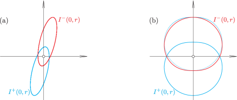
Figure 1. (a) Let $Q=[5,~{}-1;-1,~{}1]$ and $b=(1/5,1/2)$ in Example 5.2 (a). The forward and backward balls (which are ellipses) with the same radius can be translated to each other. (b) Let $\alpha\approx 35^{o}$ and $v=6$ in Example 5.2 (b). The forward and backward balls with the same radius cannot be translated to each other.

6. Appendix: Proof of Lemma 2.1

We first recall the quantitative Young inequality (see e.g. Cianchi [14]), i.e., if $r\geq 2$ and $\frac{1}{r}+\frac{1}{r^{\prime}}=1$, one has

$$uv\leq\frac{1}{r}u^{r}+\frac{1}{r^{\prime}}v^{r^{\prime}}-\frac{1}{r}|u-v^{\frac{1}{r-1}}|^{r}\ \ {\rm for\ every}\ u,v\geq 0.$$ (6.1)

(i) Let $p\in(0,\infty)$ and let us assume first that $pn\geq 1.$ Applying inequality (6.1) for $r=\frac{p}{\tilde{p}}=pn+1\geq 2$ and $r^{\prime}=\frac{1}{\tilde{p}n}$, we have that

$$\frac{\left[\mathcal{M}_{s}^{\tilde{p}}(\frac{1}{c},\frac{1}{d})\right]^{\tilde{p}}}{\left[\mathcal{M}_{s}^{p}(a,b)\right]^{\tilde{p}}\left[\mathcal{M}_{s}^{\frac{1}{n}}(\frac{1}{ac},\frac{1}{bd})\right]^{\tilde{p}}} = \frac{(1-s)^{\frac{1}{r}}a^{\tilde{p}}}{\left[\mathcal{M}_{s}^{p}(a,b)\right]^{\tilde{p}}}\frac{(1-s)^{\frac{1}{r^{\prime}}}(\frac{1}{ac})^{\tilde{p}}}{\left[\mathcal{M}_{s}^{\frac{1}{n}}(\frac{1}{ac},\frac{1}{bd})\right]^{\tilde{p}}}+\frac{s^{\frac{1}{r}}b^{\tilde{p}}}{\left[\mathcal{M}_{s}^{p}(a,b)\right]^{\tilde{p}}}\frac{s^{\frac{1}{r^{\prime}}}(\frac{1}{bd})^{\tilde{p}}}{\left[\mathcal{M}_{s}^{\frac{1}{n}}(\frac{1}{ac},\frac{1}{bd})\right]^{\tilde{p}}}$$

$$\leq \frac{1}{r}\frac{(1-s)a^{\tilde{p}r}}{\left[\mathcal{M}_{s}^{p}(a,b)\right]^{\tilde{p}r}}+\frac{1}{r^{\prime}}\frac{(1-s)(\frac{1}{ac})^{\tilde{p}r}}{\left[\mathcal{M}_{s}^{\frac{1}{n}}(\frac{1}{ac},\frac{1}{bd})\right]^{\tilde{p}r}}$$

$$-\frac{1}{r}\left|\frac{(1-s)^{\frac{1}{r}}a^{\tilde{p}}}{\left[\mathcal{M}_{s}^{p}(a,b)\right]^{\tilde{p}}}-\left(\frac{(1-s)^{\frac{1}{r^{\prime}}}(\frac{1}{ac})^{\tilde{p}}}{\left[\mathcal{M}_{s}^{\frac{1}{n}}(\frac{1}{ac},\frac{1}{bd})\right]^{\tilde{p}}}\right)^{\frac{1}{r-1}}\right|^{r}$$

$$+\frac{1}{r}\frac{sb^{\tilde{p}r}}{\left[\mathcal{M}_{s}^{p}(a,b)\right]^{\tilde{p}r}}+\frac{1}{r^{\prime}}\frac{s(\frac{1}{bd})^{\tilde{p}r}}{\left[\mathcal{M}_{s}^{\frac{1}{n}}(\frac{1}{ac},\frac{1}{bd})\right]^{\tilde{p}r}}$$

$$-\frac{1}{r}\left|\frac{s^{\frac{1}{r}}b^{\tilde{p}}}{\left[\mathcal{M}_{s}^{p}(a,b)\right]^{\tilde{p}}}-\left(\frac{s^{\frac{1}{r^{\prime}}}(\frac{1}{bd})^{\tilde{p}}}{\left[\mathcal{M}_{s}^{\frac{1}{n}}(\frac{1}{ac},\frac{1}{bd})\right]^{\tilde{p}}}\right)^{\frac{1}{r-1}}\right|^{r}$$

$$= 1-\frac{1}{r}(1-s)\left|\left[\mathcal{M}_{s}^{-p}\left(1,\frac{a}{b}\right)\right]^{\tilde{p}}-\left[\mathcal{M}_{s}^{-\frac{1}{n}}\left(1,\frac{bd}{ac}\right)\right]^{\frac{\tilde{p}}{pn}}\right|^{r}$$

$$-\frac{1}{r}s\left|\left[\mathcal{M}_{s}^{-p}\left(\frac{b}{a},1\right)\right]^{\tilde{p}}-\left[\mathcal{M}_{s}^{-\frac{1}{n}}\left(\frac{ac}{bd},1\right)\right]^{\frac{\tilde{p}}{pn}}\right|^{r}.$$

By rearranging the latter estimate, we obtain

$$\left[\mathcal{M}_{s}^{p}(a,b)\right]^{\tilde{p}}\left[\mathcal{M}_{s}^{\frac{1}{n}}\left(\frac{1}{ac},\frac{1}{bd}\right)\right]^{\tilde{p}} \geq \left[\mathcal{M}_{s}^{\tilde{p}}\left(\frac{1}{c},\frac{1}{d}\right)\right]^{\tilde{p}}+\frac{1}{r}\left[\mathcal{M}_{s}^{p}(a,b)\right]^{\tilde{p}}\left[\mathcal{M}_{s}^{\frac{1}{n}}\left(\frac{1}{ac},\frac{1}{bd}\right)\right]^{\tilde{p}}\times$$

$$\times\left[(1-s)\left|\left[\mathcal{M}_{s}^{-p}\left(1,\frac{a}{b}\right)\right]^{\tilde{p}}-\left[\mathcal{M}_{s}^{-\frac{1}{n}}\left(1,\frac{bd}{ac}\right)\right]^{\frac{\tilde{p}}{pn}}\right|^{r}\right.+$$

$$\ \ \ \ \ \ +s\left.\left|\left[\mathcal{M}_{s}^{-p}\left(\frac{b}{a},1\right)\right]^{\tilde{p}}-\left[\mathcal{M}_{s}^{-\frac{1}{n}}\left(\frac{ac}{bd},1\right)\right]^{\frac{\tilde{p}}{pn}}\right|^{r}\right].$$

Since $\frac{1}{p}+n=\frac{1}{\tilde{p}}$ we can apply (2.1) to get

$$\mathcal{M}_{s}^{p}(a,b)\mathcal{M}_{s}^{\frac{1}{n}}\left(\frac{1}{ac},\frac{1}{bd}\right)\geq\mathcal{M}_{s}^{\tilde{p}}\left(\frac{1}{c},\frac{1}{d}\right).$$

Using this estimate on the right hand side of the above inequality and the definition of $G_{s}^{p,n}(a,b,c,d)$, it follows that

$$\left[\mathcal{M}_{s}^{p}(a,b)\right]^{\tilde{p}}\left[\mathcal{M}_{s}^{\frac{1}{n}}\left(\frac{1}{ac},\frac{1}{bd}\right)\right]^{\tilde{p}} \geq \left[\mathcal{M}_{s}^{\tilde{p}}\left(\frac{1}{c},\frac{1}{d}\right)\right]^{\tilde{p}}\left(1+\frac{p}{r}G_{s}^{p,n}(a,b,c,d)\right).$$

Note that $\frac{1}{\tilde{p}}=\frac{pn+1}{p}>1;$ then we may apply to the latter estimate Bernoulli’s inequality (i.e., $(1+z)^{r}\geq 1+rz$ for $r\geq 1$ and $z\geq-1$), obtaining

$$\mathcal{M}_{s}^{p}(a,b)\mathcal{M}_{s}^{\frac{1}{n}}\left(\frac{1}{ac},\frac{1}{bd}\right) \geq \mathcal{M}_{s}^{\tilde{p}}\left(\frac{1}{c},\frac{1}{d}\right)\left(1+\frac{p}{r\tilde{p}}G_{s}^{p,n}(a,b,c,d)\right).$$

Since $r\tilde{p}=p$ and

$$\mathcal{M}_{s}^{\tilde{p}}\left(\frac{1}{c},\frac{1}{d}\right)=\left[\mathcal{M}_{s}^{-\tilde{p}}(c,d)\right]^{-1},$$

the desired relation follows. The case $pn\leq 1$ follows in the same way.

If $p\in(-\frac{1}{n},0).$ Since $-\tilde{p}=-\frac{p}{pn+1}\in(0,\infty)$ and $p=\frac{\tilde{p}}{\tilde{p}n+1}$, we can apply the previous estimate by reversing the roles of the means.

A simple computation shows that $G_{s}^{p,n}(a,b,c,d)=0$ if and only if $\frac{a}{b}=\left(\frac{d}{c}\right)^{\frac{1}{pn+1}}.$

(ii) We first assume that $s\geq\frac{1}{2}$, i.e., $\min(s,1-s)=1-s$. We apply (6.1) with $r=\frac{1}{1-s}\geq 2$ and $r^{\prime}=\frac{1}{s}$, obtaining

$$\frac{[\mathcal{M}_{s}^{0}(\frac{1}{c},\frac{1}{d})]^{\frac{1}{n}}}{\left[\mathcal{M}_{s}^{0}(a,b)\right]^{\frac{1}{n}}[\mathcal{M}_{s}^{\frac{1}{n}}(\frac{1}{ac},\frac{1}{bd})]^{\frac{1}{n}}} = \frac{(\frac{1}{ac})^{\frac{1-s}{n}}(\frac{1}{bd})^{\frac{s}{n}}}{(1-s)(\frac{1}{ac})^{\frac{1}{n}}+s(\frac{1}{bd})^{\frac{1}{n}}}$$

$$\leq \frac{(1-s)(\frac{1}{ac})^{\frac{1}{n}}+s(\frac{1}{bd})^{\frac{1}{n}}-(1-s)|(\frac{1}{ac})^{\frac{1-s}{n}}-((\frac{1}{bd})^{\frac{s}{n}})^{\frac{1-s}{s}}|^{\frac{1}{1-s}}}{(1-s)(\frac{1}{ac})^{\frac{1}{n}}+s(\frac{1}{bd})^{\frac{1}{n}}}$$

$$= 1-(1-s)\frac{|(\frac{1}{ac})^{\frac{1-s}{n}}-(\frac{1}{bd})^{\frac{1-s}{n}}|^{\frac{1}{1-s}}}{(1-s)(\frac{1}{ac})^{\frac{1}{n}}+s(\frac{1}{bd})^{\frac{1}{n}}}$$

$$= 1-(1-s)\left|\left[{\mathcal{M}_{s}^{-\frac{1}{n}}\left(1,\frac{bd}{ac}\right)}\right]^{\frac{1-s}{n}}-\left[{\mathcal{M}_{s}^{-\frac{1}{n}}\left(\frac{ac}{bd},1\right)}\right]^{\frac{1-s}{n}}\right|^{\frac{1}{1-s}}.$$

Rearranging the above inequality, and using $\mathcal{M}_{s}^{0}(ac,bd)\geq\mathcal{M}_{s}^{-\frac{1}{n}}(ac,bd)$ and the Bernoulli inequality, it follows that

$$\mathcal{M}_{s}^{0}(ac,bd)\geq\mathcal{M}_{s}^{-\frac{1}{n}}(ac,bd)\left(1+n{(1-s)}\left|\left[{\mathcal{M}_{s}^{-\frac{1}{n}}\left(1,\frac{bd}{ac}\right)}\right]^{\frac{1-s}{n}}-\left[{\mathcal{M}_{s}^{-\frac{1}{n}}\left(\frac{ac}{bd},1\right)}\right]^{\frac{1-s}{n}}\right|^{\frac{1}{1-s}}\right).$$

If $s\leq\frac{1}{2}$, we proceed in a similar way as above. Furthermore, $G_{s}^{0,n}(a,b,c,d)=0$ if and only if $ac=bd.$

(iii) We first assume that $a\geq b$. Then we have

$$\frac{[\mathcal{M}_{s}^{\frac{1}{n}}(\frac{1}{c},\frac{1}{d})]^{\frac{1}{n}}}{[\mathcal{M}_{s}^{+\infty}(a,b)]^{\frac{1}{n}}[\mathcal{M}_{s}^{\frac{1}{n}}(\frac{1}{ac},\frac{1}{bd})]^{\frac{1}{n}}} = 1+s\frac{(b^{\frac{1}{n}}-a^{\frac{1}{n}})}{(abd)^{\frac{1}{n}}}\left[\mathcal{M}_{s}^{-\frac{1}{n}}(ac,bd)\right]^{\frac{1}{n}}.$$

After a rearrangement, Bernoulli’s inequality and (2.1) give the required inequality. The same can be done for $a\leq b.$ Moreover, $G_{s}^{+\infty,n}(a,b,c,d)=0$ if and only if $a=b.$

The proof of (iv) directly follows by (iii); we left it to the interested reader. $\square$

Acknowledgement. We express our gratitude to Alessio Figalli and Cédric Villani for their useful comments on the earlier version of the manuscript. A. Kristály is grateful to the Mathematisches Institute of Bern for the warm hospitality where this work has been initiated. We also thank the anonymous Referee for her/his valuable comments that greatly improved the presentation of the manuscript.

Mathematisches Institute, Universität Bern, Sidlerstrasse 5, 3012 Bern, Switzerland.
Email: zoltan.balogh@math.unibe.ch

Department of Economics, Babeş-Bolyai University, Str. T. Mihali 58-60, 400591 Cluj-Napoca, Romania;
Institute of Applied Mathematics, Óbuda University, Bécsi út 96, 1034 Budapest, Hungary.
Email: alex.kristaly@econ.ubbcluj.ro; kristaly.alexandru@nik.uni-obuda.hu

References

- [1] K. Bacher, On Borell-Brascamp-Lieb inequalities on metric measure spaces, Potential Anal. 33 (2010), no. 1, 1–15.
- [2] K. M. Ball, K. J. Böröczky, Stability of some versions of the Prékopa-Leindler inequality, Monatsh. Math. 163 (2011), no. 1, 1–14.
- [3] K. M. Ball, K. J. Böröczky, Stability of the Prékopa-Leindler inequality, Mathematika 56 (2010), no. 2, 339–356.
- [4] D. Bao, S. S. Chern, Z. Shen, Introduction to Riemann–Finsler Geometry, Graduate Texts in Mathematics, 200, Springer Verlag, 2000.
- [5] R. L. Bishop, R. J. Crittenden, Geometry of manifolds. Reprint of the 1964 original. AMS Chelsea Publishing, Providence, RI, 2001.
- [6] S. G. Bobkov, M. Ledoux, From Brunn-Minkowski to Brascamp-Lieb and to logarithmic Sobolev inequalities, Geom. Funct. Anal. 10 (2000), no. 5, 1028–1052.
- [7] W. M. Boothby, An introduction to differentiable manifolds and Riemannian geometry. Second edition. Pure and Applied Mathematics, 120. Academic Press, Inc., Orlando, FL, 1986.
- [8] C. Borell, Convex set functions in d-space, Period. Math. Hung. 6 (1975), 111–136.
- [9] K. J. Böröczky, E. Lutwak, D. Yang, G. Zhang, The log-Brunn-Minkowski inequality, Adv. Math. 231 (2012), no. 3-4, 1974–1997.
- [10] H.J. Brascamp, E.H. Lieb, On extensions of the Brunn-Minkowski and Prékopa-Leindler theorems, including inequalities for log concave functions and with an application to the diffusion equation, J. Funct. Anal. 22 (1976), no. 4, 366–389.
- [11] D. Bucur, I. Fragalà, Lower bounds for the Prékopa-Leindler deficit by some distances modulo translations, J. Convex Anal. 21 (2014), no. 1, 289–305.
- [12] L. Caffarelli, The regularity of mappings with a convex potential, J. Amer. Math. Soc. 5 (1992), no. 1, 99–104.
- [13] M. Christ, Near equality in the Brunn-Minkowski inequality, preprint. Available online at: https://arxiv.org/abs/1207.5062.
- [14] A. Cianchi, Sharp Morrey-Sobolev inequalities and the distance from extremals, Trans. Amer. Math. Soc. 360 (2008), no. 8, 4335–4347.
- [15] A. Colesanti, G. Livshyts, A. Marsiglietti, On the stability of Brunn-Minkowski type inequalities, J. Funct. Analysis, 273 (2017), no. 3, 1120–1139.
- [16] D. Cordero-Erausquin, Inégalité de Prékopa-Leindler sur la sphère, C. R. Acad. Sci. Paris Sér. I Math. 329 (1999), no. 9, 789–792.
- [17] D. Cordero-Erausquin, R. J. McCann, M. Schmuckenschläger, A Riemannian interpolation inequality à la Borell, Brascamp and Lieb, Invent. Math. 146 (2001), no. 2, 219–257.
- [18] S. Dancs, B. Uhrin, On a class of integral inequalities and their measure-theoretic consequences, J. Math. Anal. Appl. 74 (1980), 388–400.
- [19] S. Dancs, B. Uhrin, On the conditions of equality in an integral inequality, Publ. Math. (Debrecen) 29 (1982), 117–132.
- [20] M. P. do Carmo, Riemannian Geometry, Birkhäuser, Boston, 1992.
- [21] S. Dubuc, Critères de convexité et inégalités intègrales, Ann. Inst. Fourier (Grenoble) 27 (1977) no. 1, 135–165.
- [22] A. Figalli, D. Jerison, Quantitative stability of the Brunn-Minkowski inequality for sets of equal volume, Chin. Ann. Math. Ser. B 38 (2017), no. 2, 393–412.
- [23] A. Figalli, D. Jerison, Quantitative stability for the Brunn-Minkowski inequality, Adv. Math., 314 (2017), 1–47.
- [24] A. Figalli, D. Jerison, A sharp Freiman type estimate for semisums in , preprint. Available on-line at: https://people.math.ethz.ch/ afigalli/submitted-pdf/A-sharp-freiman-type-estimate-for-semisums-in-rn.pdf
- [25] A. Figalli, F. Maggi, A. Pratelli, A mass transportation approach to quantitative isoperimetric inequalities, Invent. Math. 182 (2010), no. 1, 167–211.
- [26] A. Figalli, F. Maggi, A. Pratelli, A refined Brunn-Minkowski inequality for convex sets, Ann. Inst. H. Poincaré Anal. Non Linéaire 26 (2009), no. 6, 2511–2519.
- [27] R. J. Gardner, The Brunn-Minkowski inequality, Bull. Amer. Math. Soc. (N.S.) 39 (2002), no. 3, 355–405.
- [28] D. Ghilli, P. Salani, Quantitative Borell-Brascamp-Lieb inequalities for power concave functions, J. Convex Anal. 24 (2017), No. 3. Available online at: http://www.heldermann.de/JCA/JCA24/jca24.htm
- [29] H. Knothe, Contributions to the theory of convex bodies, Michigan Math. J. 4 (1957), 39–52.
- [30] A. Kristály, A sharp Sobolev interpolation inequality on Finsler manifolds, J. Geom. Anal. 25 (2015), no. 4, 2226–2240.
- [31] J. Lott, C. Villani, Ricci curvature for metric-measure spaces via optimal transport, Ann. of Math. (2) 169 (2009), no. 3, 903–991.
- [32] M. Matsumoto, A slope of a mountain is a Finsler surface with respect to a time measure, J. Math. Kyoto Univ. 29 (1989), 17–25.
- [33] R. J. McCann, Polar factorization of maps on Riemannian manifolds, Geom. Funct. Anal. 11 (2001), no. 3, 589–608.
- [34] R. J. McCann, A convexity principle for interacting gases, Adv. Math. 128 (1997), no. 1, 153–179.
- [35] R. J. McCann, A convexity theory for interacting gases and equilibrium crystals, ProQuest LLC, Ann Arbor, MI, 1994, Thesis (Ph.D.) Princeton University.
- [36] E. Milman, L. Rotem, Complemented Brunn-Minkowski inequalities and isoperimetry for homogeneous and non-homogeneous measures, Adv. Math. 262 (2014), 867–908.
- [37] V. D. Milman, G. Schechtman, Asymptotic theory of finite-dimensional normed spaces, With an appendix by M. Gromov. Springer-Verlag, Berlin, 1986.
- [38] S. Ohta, Finsler interpolation inequalities, Calc. Var. Partial Differential Equations 36 (2009), no. 2, 211–249.
- [39] G. Randers, On an asymmetrical metric in the fourspace of general relativity, Phys. Rev. (2) 59, (1941), 195–199.
- [40] T. Rajala, Large porosity and dimension of sets in metric spaces, Ann. Acad. Sci. Fenn. Math. 34 (2009), no. 2, 565–581.
- [41] A. Rossi, Borell-Brascamp-Lieb inequalities: rigidity and stability, PhD Thesis in Mathematics, Informatics, Statistics - Università di Firenze, 2018.
- [42] A. Rossi, P. Salani, Stability for Borell-Brascamp-Lieb inequalities, Geometric aspects of functional analysis, 339–363, Lecture Notes in Math., 2169, Springer, Cham, 2017.
- [43] A. Rossi, P. Salani, Stability for a strengthened Borell-Brascamp-Lieb inequality, Appl. Anal., 2018, to appear. DOI: 10.1080/00036811.2018.1451645.
- [44] T. Sakai, Riemannian geometry. Translations of Mathematical Monographs, 149. American Mathematical Society, Providence, RI, 1996.
- [45] Z. Shen, Volume comparison and its applications in Riemann-Finsler geometry, Adv. Math. 128 (1997), no. 2, 306–328.
- [46] H. Steinhaus, Sur les distances des points dans les ensembles de mesure positive, Fund. Math. 1 (1920), 93–104.
- [47] K.-T. Sturm, On the geometry of metric measure spaces. II, Acta Math. 196 (2006), no. 1, 133–177.
- [48] C. Villani, Optimal transport, Old and new. Grundlehren der Mathematischen Wissenschaften [Fundamental Principles of Mathematical Sciences], vol. 338, Springer-Verlag, Berlin, 2009.
- [49] C. Villani, Topics in optimal transportation. Graduate Studies in Mathematics, 58. American Mathematical Society, Providence, RI, 2003.