Blind Demixing and Deconvolution at Near-Optimal Rate

Abstract

We consider simultaneous blind deconvolution of $r$ source signals from their noisy superposition, a problem also referred to blind demixing and deconvolution. This signal processing problem occurs in the context of the Internet of Things where a massive number of sensors sporadically communicate only short messages over unknown channels. We show that robust recovery of message and channel vectors can be achieved via convex optimization when random linear encoding using i.i.d. complex Gaussian matrices is used at the devices and the number of required measurements at the receiver scales with the degrees of freedom of the overall estimation problem. Since the scaling is linear in $r$ our result significantly improves over recent works.

1 Introduction

Recent progress regarding recovery problems for low-complexity structures in high-dimensional data have shown that a substantial reduction in sampling and storage complexity can be achieved in many relevant non–adaptive linear signal separation and estimation problems, in particular in the case of randomized strategies. This includes the recovery of sparse and compressible vectors (often referred to as compressed sensing) [CRT06, Don06], low–rank matrices [RFP10], and higher–order tensors from subsampled linear measurements [RSS17], as well as the compressive demixing of multiple source signals [MT14]. An important step in many of such vector and matrix recovery problems is to establish computational tractability in the sense of complexity theory; a common strategy to achieve this is to show that, under appropriate assumptions on the measurement map, the reconstruction problem can be recast as a tractable convex program.

In practice, however, one faces additional difficulties. Namely, the data acquisition process has to cope with uncalibrated measurement devices depending on further unknown parameters. In many such scenarios one can only sample the output of an unknown or partially known linear system. In such cases the object/signal $s$ to recover is coupled with the unknown or partially known environment $w$ in a multiplicative way giving rise to a bilinear inverse problem, i.e., solve for $s$ and $w$ given a bilinear combination $\mathcal{B}(w,s)$. Relevant examples are when the effective sensing matrix might be subject to uncertainties [BN07, HS10, CS11, GE11], or signals might have been transmitted through individual channels whose properties are not completely known [WP98]. Our current understanding of these blind information retrieval tasks is at the very beginning and usually it forces one therefore to operate at sub-optimal sensing rates, or else incur significant reconstruction errors due to model mismatch. The situation is all the more unsatisfactory, as such blind sampling problems are often much closer to practical applications than the original linear models.

1.1 Blind Deconvolution

The prototypical bilinear mapping, practically relevant in many applications, is the convolution

$$w\ast s:=(\sum_{j=1}^{L}{w}_{j}s_{k-j})_{k=1}^{L}.$$

For technical reasons we will consider the circular convolution, where the index difference $k-j$ is considered modulo $L$. The classical convolution can be reduced to this setup by appropriate zero padding. Then the corresponding inverse problem, that is, the problem of recovering $s$ and $w$ from their convolution up to inherent ambiguities, is known as blind deconvolution [Hay94]. The precise role of $s$ and $w$ depends on the underlying application. In imaging, for example, the signal vector $s$ typically represents the image and $w$ is an unknown blurring kernel [SCI75]. In communication engineering, $w$ represents the channel parameters and the task is to demodulate and decode the signal information $s$ only having access to the channel output $w\ast s$, and the important question is how much overhead is required for coping with the unknown impulse response $w$ of the communication channel [God80].

Obviously, without further constraining $s$ and $w$ the convolution $(s,w)\rightarrow w\ast s$ has many more degrees of freedom than measurements and is hence far from injective, exhibiting various kinds of ambiguities. The goal must then be to eliminate these ambiguities as much as possible by imposing structural constraints on the signal and the channel paramters. It should be noted that a scaling ambiguity will always remain, as any bilinear mapping $\mathcal{B}$ satisfies $\mathcal{B}(s,w)=\mathcal{B}(\lambda s,w/\lambda)$ for any $0\neq\lambda\in\mathbb{C}$ and can hence be injective only up to a multiplicative factor. Specific scenarios can give rise to additional ambiguities, as it has been investigated in [CM14b]. For more detailed discussions of ambiguities in the one-dimensional case such as shifts or reflections, see [CM14a] and [WJPH16]. In any case, additional constraints like sparsity and subspace priors, depending on the specific application, are necessary to make blind deconvolution feasible. It has been shown that sparsity in the canonical basis alone is not sufficient for these purposes [CM15], and for generic bases, the subspace dimensions and sparsity levels that yield injectivity have been exactly classified [LLB15, LLB17, KK17].

Even when injectivity can be established, this does not directly yield a tractable reconstruction scheme. While a number of works have studied algorithms for recovery (see, e.g.,[CW00, LWDF, AF13]), the focus has mostly been on algorithmic performance rather than on recoverability guarantees. The search for algorithms allowing for guaranteed recovery has recently shown significant progress by taking a compressed sensing viewpoint, namely aiming to choose remaining degrees of freedom to reduce the degree of ill-posedness. The first near-optimal rigourous recovery guarantees in a randomized setting have been established in [ARR14] with high probability under the assumption that both the signal and the channel parameters lie in subspaces of small dimension, and one of them is chosen at random. The main idea was to exploit that any bilinear map $\mathcal{B}(w,s)$ can be represented as a linear map in the outer product $ws^{T}$ of the two input vectors (this approach is often referred to as lifting) and hence analyzed using methods from the theory of low rank matrix recovery. More precisely, exploiting the fact that the (normalized, unitary) $L\times L$ discrete Fourier matrix $F$ diagonalizes the circular convolution to establish the representation

$$w\ast s:=\sqrt{L}\cdot F^{*}\text{diag}(Fw)Fs,$$ (1.1)

with $\text{diag}(v)$ denoting the diagonal matrix with the entries of $v$ on its diagonal.

Under the subspace model, where both the signal $s$ and the vector of channel parameters are assumed to lie in a known low-dimensional subspace and hence can be represented as $w=F^{*}Bh$ and $s=F^{*}C\overline{x}/\sqrt{L}$, for given $B\in\mathbb{C}^{L\times K}$ and $C\in\mathbb{C}^{L\times N}$, this translates to

$$y:=F(w\ast s)=\text{diag}(Bh)C\overline{x}=:\mathcal{A}(hx^{*}),$$ (1.2)

where $\mathcal{A}$ is a linear map and $M^{*}$ denotes the adjoint of a matrix $M$, that is, its conjugate transpose. This formulation yields a low rank recovery problem, as of all potential matrices giving rise to measurements $y$, the rank one matrix $hx^{*}$ is the one of the lowest rank. Even though recovering a low rank matrix from linear measurements is known to be, in general, NP-hard [CG84], it has been shown that under appropriate random measurement models, one can establish recovery guarantees for tractable algorithms with high probability [CP11, Gro11]. While the results in these works require more randomness than what is available in the convolution setup due to the structure imposed by (1.2) and hence do not apply directly, Ahmed, Recht, and Romberg [ARR14] derived recovery guarantees for blind deconvolution. Their result assumes that (i) $C$ has independent standard Gaussian entries and that (ii) $B^{*}B=1$ and $B$ is incoherent in two ways, namely that $\mu^{2}_{\max}:=\frac{L}{K}\max_{\ell}\|b_{\ell}\|^{2}_{\ell_{2}}$ and $\mu^{2}_{h}=L\cdot\max_{1\leq\ell\leq L}|b_{\ell}^{*}h|^{2}$ are sufficiently small ($b_{\ell}$ are the columns of $B^{*}$). Under these assumptions, they showed that the unknown real $K\times N$–matrix $hx^{*}$ can be recovered with overwhelming probability by nuclear norm minimization, that is, via the semidefinite program

$$\min\lVert X\rVert_{*}\quad\text{s.t.}\quad\mathcal{A}(X)=y.$$ (1.3)

Here, $\lVert X\rVert_{*}$ denotes the nuclear norm of the matrix $X$, which is defined to be the sum of its singular values.

Although nuclear norm minimization is computational tractable, the lifted representation drastically increases the size of the signal to be recovered. Consequently, the resulting algorithm will be too slow for most practical applications. The theoretical analysis of nuclear norm minimization has, however, paved the way for more efficient algorithms with similar guarantees. Namely, the recent work [LLSW16] demonstrates that a gradient-based algorithm with a suitable initialization can be used without lifting and in the regime $\mu^{2}_{h}\max(K,N)\lesssim L/\log^{2}(L)$ which comes with considerably reduced complexity.

Finally, typical channel impulse responses $h$ exhibit further structural properties such as sparsity, which should be used as well. However, the challenging extension of these works to sparsity models seems to be much more involved. The difficulty with such models is that the lifted representation is both sparse and of low rank, and no straightforward tractable convex relaxation is known. In particular, minimizing convex combinations of nuclear and $\ell_{1}$-norm regularizers has been shown to yield provably suboptimal recovery performance [OJF⁺15]. Research regarding alternative convex surrogates as for example in [ROV14] is only in its beginnings. For this reason, some recent approaches ignore the rank constraint, just aiming for sparsity, as investigated for the $\ell_{1}$–approach (sparse lift) in [LS15b] and for the mixed $\ell_{1}/\ell_{2}$-case in [Fliar].

On the other hand, the search for non-convex alternatives to overcome this obstacle is an active area of research. In particular, local convergence guarantees as well as global convergence guarantees for peaky signals have been derived in [LLJB17] for the sparse power factorization method, an alternating minimization approach originally introduced in [LWB13], for the context of deconvolution. The near-optimal recovery guarantees build on some property similar to the restricted isometry property, which has been derived in [LJ15] (for both inputs lying in random subspaces). The search for global recovery guarantees in the sparsity model without peakiness assumptions, however, remains open.

1.2 Simultaneous Demixing and Blind Deconvolution

The extension of the model we shall consider here is blind deconvolution and simultaneously demixing multiple source signals. This setting is motivated by recent challenges in future wireless multi–terminal communication scenarios for uncoordinated sporadic communication [WBSJ15, JW15]. We consider the prototypical case of $R$ transmitters each having an individual information message encoded into the vector $x_{i}\in\mathbb{C}^{N_{i}}$ for $i=1,\ldots,R$ using, for example, classical modulation alphabets and error–correcting codes. In fact, such data could be independent user data payloads or even correlated sensor readings on a common source. For reasons of simplicity, we focus on the case of independent data sources. Each transmitter generates its transmit signal $s_{i}=F^{*}C_{i}\overline{x}_{i}/\sqrt{L}\in\mathbb{C}^{L}$ by multiplying (linearly encoding) its complex–valued (conjugated) message vector $\overline{x}_{i}$ by an $L\times N_{i}$ matrix $F^{*}C_{i}/\sqrt{L}$ which is then transmitted into the shared channel. Note that, from the perspective of communication engineering, this procedure has been simplified to facilitate the analysis. In a more advanced setting one could consider a directly randomized mapping from bits to sequences in $\mathbb{C}^{L}$. Now consider a single receiver, for example a base station. Each transmitter $i$ has its individual impulse response $w_{i}$ describing the channel propagation conditions to this base station. For simplicity we consider a low–mobility scenario where, for appropriate block length $L$, the channel is time–invariant and can be modeled by a convolution of the transmit signal with a channel impulse response $w_{i}$. Furthermore, with cyclic extensions and zero-padding at the transmitter such a signal propagation can then be modeled as a circular convolution. To incorporate further structure for the channel impulse response we write it as $w_{i}=F^{*}B_{i}h_{i}$ where $B_{i}\in\mathbb{C}^{L\times K_{i}}$. A reasonable assumption for our application is that the unknown coefficients $h_{i}$ are located on the first samples since the path delays in the channel are usually much shorter than the frame length $L$. In this case $F^{*}B_{i}$ is a truncated identity, i.e., $B_{i}^{*}B_{i}=\text{Id}$.

In practice, since the desired deployment scenario is uncoordinated and sporadic, only a small fraction of size $r$ of $R$ devices are online and transmitting data. We assume for this work that the receiver is able to detect the activity pattern correctly (which can be achieved through a separate control channel, see for example [KJ16] for a certain approach). One can even detect activity simultaneously with data. However, algorithms for blind deconvolution and demixing are usually quite complex from practical and computational aspects and it is desired to reduce the problem size as much as possible already from the beginning. This means, restricted and resorting to the active set, the receiver observes the noisy superposition

$$y=\sum_{i=1}^{r}F(w_{i}\ast s_{i})+e=\sum_{i=1}^{r}\text{diag}(B_{i}h_{i})C_{i}\overline{x}_{i}+e=\sum_{i=1}^{r}\mathcal{A}_{i}(h_{i}x_{i}^{*})+e$$ (1.4)

of $r$ signal contributions where the vector $e\in\mathbb{C}^{L}$ denotes additive noise.

The conventional approach is (i) to design the matrices $C_{i}$ is such a way that resources are used exclusively by $\mathcal{O}(R)$ devices which requires considerable processing, resource planning and allocation algorithms and (ii) estimate the channel from pilot signals during a calibration phase prior to data transmission. However, in an increasing number of new applications the typical data traffic consists only of short messages (status updates or sensor data) yielding a sporadic traffic type and then the overall communication in a network is then considerable dominated by control data.

In [LS15a] it has therefore been proposed to consider the scenario of simultaneous blind deconvolution and demixing of multiple signals from its superposition $y$, which we will also study in this paper. Demixing by convex programming methods has been intensively investigated in the fields of “sine and spikes” (and pairs of bases) decompositions, see [DH01] and [ALMT14], and in the field of sparse and low–rank decomposition, see, e.g., the work [CSPW09]. More generally, as for example outlined in [MT17] and [WGMM13], a convex approach consists of minimizing the sum of the individual regularizers over all signal formations which are conform with the model and consistent with the observations. To this end, assuming a priori that $\lVert e\rVert_{\ell_{2}}\leq\tau$, we consider the convex optimization problem

$$\min\sum_{i=1}^{r}\lVert X_{i}\rVert_{*}\quad\text{s.t.}\quad\lVert\sum_{i=1}^{r}\mathcal{A}_{i}(X_{i})-y\rVert_{\ell_{2}}\leq\tau.$$ (1.5)

According to [MT17], reliable convex demixing is possible whenever (i) the signal contributions are incoherent to each other and (ii) the number of observations is sufficiently above the sum of effective dimensions of the descent cones of the individual regularizers at the unknown ground truth. Since the rank-one matrix $X_{i}=h_{i}x^{*}_{i}$ has effective dimension $K_{i}+N_{i}$ this amounts to $\mathcal{O}(r(K+N))$ observations, where $K=\max_{i}(K_{i})$ and $N=\max_{i}(N_{i})$. First results and guarantees, based on the incoherence between the mappings $\mathcal{A}_{i}$ which explicitly occur in blind deconvolution (1.4) with random $C_{i}$’s are worked out in [LS15a]. The result in this paper states that if (up to logarithmic orders) $L=\mathcal{O}(r^{2}\max(K,N))$ the minimizer $(\hat{X}_{1},\dots,\hat{X}_{r})$ of the program (1.5) satisfies with high probability that

$$\sum_{i=1}^{r}\|\hat{X}_{i}-X_{i}^{0}\|^{2}_{F}\lesssim r^{2}\cdot\max\left\{K;N\right\}\tau^{2}$$ (1.6)

Hence, for $\tau=0$ the ground truth $(\hat{X}^{0}_{1},\dots,\hat{X}^{0}_{r})$ is recovered exactly. However, the embedding dimension does not quite match the effective dimension, which would suggest a linear dependence on $r$. Ling and Strohmer suggested that this mismatch is a proof artifact, observing numerically that linear dependence on $r$. In this paper, we will analytically justify these observations. In the special case of partial (low-frequency) Fourier matrices $B_{i}$ mentioned above, our main result, Theorem 2.5, reads as follows.

Theorem 1.1.

Let $\omega\geq 1$ and set $\mu^{2}_{h}=L\max_{i,l}|b^{*}_{i,\ell}h_{i}|^{2}$. Assume $\lVert e\rVert_{\ell_{2}}\leq\tau$ and that

$$L\geq C_{\omega}r\left(K\log K+N\mu^{2}_{h}\right)\log^{3}L,$$ (1.7)

where $C_{\omega}$ is a universal constant only depending on $\omega$. Then with probability at least $1-\mathcal{O}\left(L^{-\omega}\right)$ the minimizer $\hat{X}$ of the recovery program (1.5) satisfies

$$\sum_{i=1}^{r}\|\hat{X}_{i}-X_{i}^{0}\|^{2}_{F}\lesssim r\cdot\max\left\{1;\frac{rKN}{L}\right\}\log(L)\ \tau^{2}.$$ (1.8)

Shortly before completion of this manuscript Ling and Strohmer presented recovery guarantees for (considerably more efficient) nonconvex gradient (Wirtinger) based methods [LS17], again with quadratic scaling in $r$. Again they conjecture linear dependence, as observed in their numerical experiments. We also include some numerical experiments in Section 6 at the end that illustrate the linear dependence. We expect that our paper at hand will pave the way to an optimized parameter dependence also for more efficient algorithms.

2 General Framework and Main Result

2.1 Notation

Before we describe the mathematical model we introduce some basic notation. For complex numbers $z\in\mathbb{C}$ we denote its conjugate by $\bar{z}$ and write $\text{Re }z$ and $\text{Im }z$ for the real and imaginary part. Similarly, for a vector $w=\left(w[1],\ldots,w[n]\right)\in\mathbb{C}^{n}$ we use the notation $\text{Re }w=\left(\text{Re }w[1],\ldots,\text{Re }w[n]\right)$ and $\text{Im }w=\left(\text{Im }w[1],\ldots,\text{Im }w[n]\right)$. For a matrix $A\in\mathbb{C}^{d_{1}\times d_{2}}$ we will denote its adjoint by $A^{*}$ and (for $d_{1}=d_{2}$) its trace by $\text{Tr}\,\left(A\right)$. For matrices $A,B\in\mathbb{C}^{d_{1}\times d_{2}}$ we will define the inner product by $\langle A,B\rangle_{F}=\text{Tr}\,\left(AB^{*}\right)$. The Frobenius norm of $A$ is $\|A\|^{2}_{F}=\langle A,A\rangle_{F}$ and $\|A\|_{2\rightarrow 2}$ denotes its operator norm. If $\mathcal{B}$ is a linear operator mapping matrices to vectors or matrices, we will denote its operator norm by $\|\cdot\|_{F\rightarrow 2}$ or $\|\cdot\|_{F\rightarrow F}$, respectively. The nuclear norm of the matrix $A$, which is defined as the sum of its singular values, will be denoted by $\|A\|_{\ast}$. Note that the notation for $\|\cdot\|_{\ast}$, $\lVert\cdot\rVert_{F}$ and $\langle\cdot,\cdot\rangle_{F}$ will be used later in a more generalized setting, as will be pointed out in the next section. The matrix $\text{Id}_{d}$ will denote the identity matrix in $\mathbb{C}^{d\times d}$. If no confusion can arise, we will suppress $d$ and write Id instead of $\text{Id}_{d}$. For a vector $v\in\mathbb{C}^{d}$ $\text{diag}\left(v\right)$ denotes the matrix whose diagonal entries are given by $v$. Furthermore, $\|v\|_{\ell_{2}}$ denotes the $\ell_{2}$-norm of this vector, i.e. $\|v\|^{2}_{\ell_{2}}=\langle v,v\rangle=\text{Tr}\,\left(vv^{*}\right)$.

By $\mathbb{P}\left(E\right)$ we will denote the probability of an event $E$. For any $N\in\mathbb{N}$ we will denote the set $\left\{1,\ldots,N\right\}$ by $[N]$. For a set $S$ we will denote its cardinality by $|S|$. The notation $\log\left(\cdot\right)$ will refer to the logarithm of base $2$. Furthermore, during the whole manuscript $C$ will denote positive numerical constants, which are independent of all other variables which appear in the text and whose value may change from line to line. Similarly, $C_{\omega}$ will denote universal numerical constants, which only depend on $\omega$. We will write $a\lesssim b$, if $a\leq Cb$ and $a\lesssim_{\omega}b$, if $a\leq C_{\omega}b$. We will write $a\sim b$, if we have $a\lesssim b$ as well as $b\lesssim a$.

2.2 The General Model

In this paper we will work with a more general model, as also studied in [LS15a], which includes the demixing-deconvolution scenario given above as special case. Assume that the vector $y\in\mathbb{C}^{L}$ of $L$ noisy measurements corresponding to inputs $\left\{h_{i}\right\}^{r}_{i=1}$, $h_{i}\in\mathbb{C}^{K_{i}}$ and $\left\{x_{i}\right\}^{r}_{i=1}$, $x_{i}\in\mathbb{C}^{N_{i}}$, is given by

$$y=\sum_{i=1}^{r}\text{diag}\left(B_{i}h_{i}\right)C_{i}\overline{x}_{i}+e.$$ (2.1)

where $e$ is additive noise, the matrices $B_{i}\in\mathbb{C}^{L\times K_{i}}$ satisfy $B^{*}_{i}B_{i}=\text{Id}_{K_{i}}$ for all $i\in[r]$, and all the entries of the random matrices $C_{i}\in\mathbb{C}^{L\times N_{i}}$ are independent and follow a standard circular-symmetric complex normal distribution $\mathcal{CN}\left(0,1\right)$ (see Appendix B for more details). The vectors $h_{i}$ are assumed to be normalized, $\|h_{i}\|_{\ell_{2}}=1$, whereas the norms of $x_{i}$ are arbitrary. (This is not restrictive as there is an inherent scaling ambiguity.) Furthermore, we set

$$K=\underset{i\in[r]}{\max}\ K_{i}\quad\text{and}\quad N=\underset{i\in[r]}{\max}\ N_{i}.$$

Let us denote by $b_{i,\ell}$ the $\ell$th column of $B^{*}_{i}$ and by $c_{i,\ell}$ the $\ell$th column of $C_{i}$. Then, the $\ell$th entry of $y$ is given by

$$y[\ell]=\sum_{i=1}^{r}b^{*}_{i,\ell}h_{i}x^{*}_{i}c_{i,\ell}+e[\ell].$$

We observe that the overall vector $y$ only depends on the outer products $h_{i}x^{*}_{i}$. Thus, we may proceed by considering a lifted representation (see, e.g., [BCEB08]). Defining for each $i\in[r]$ the operator $\mathcal{A}_{i}:\mathbb{C}^{K_{i}\times N_{i}}\longrightarrow\mathbb{C}^{L}$ via

$$\mathcal{A}_{i}\left(Z\right):=\left(b^{*}_{i,\ell}Zc_{i,\ell}\right)^{L}_{\ell=1}$$

we obtain that

$$y=\sum_{i=1}^{r}\mathcal{A}_{i}\left(h_{i}x^{*}_{i}\right)+e.$$

In the following we will use the decomposition $x_{i}=\sigma_{i}m_{i}$ where $\sigma_{i}\geq 0$ and some $m_{i}\in\mathbb{C}^{N_{i}}$ such that $\|m_{i}\|_{\ell_{2}}=1$. (If $x_{i}=0$ we set $\sigma_{i}=0$ and choose $m_{i}$ arbitrarily.) Thus, the signal to be recovered may be written as

$$X^{0}=\left(h_{1}x^{*}_{1},\ldots,h_{r}x^{*}_{r}\right)=\left(\sigma_{1}h_{1}m^{*}_{1},\ldots,\sigma_{r}h_{r}m^{*}_{r}\right)=:\left(X_{1},\ldots,X_{r}\right).$$

Define

$$\mathcal{M}:=\left\{\left(Z_{1},\ldots,Z_{r}\right):\ Z_{i}\in\mathbb{C}^{K_{i}\times N_{i}}\text{ for all }i\in\left[r\right]\right\}$$

and note that $\mathcal{M}$ is naturally equipped with the algebraic structure of a vector space, as it may be regarded as the product space of the vector spaces $\mathbb{C}^{K_{i}\times N_{i}}$. The linear operator $\mathcal{A}:\mathcal{M}\rightarrow\mathbb{C}^{L}$ is defined by

$$\mathcal{A}\left(Z\right):=\sum_{i=1}^{r}\mathcal{A}_{i}\left(Z_{i}\right)$$

for $Z=\left(Z_{1},\ldots,Z_{r}\right)\in\mathcal{M}$. The linear space $\mathcal{M}$ will be endowed with a norm and an inner product defined by

$$\langle W,Z\rangle_{F}=\sum_{i=1}^{r}\langle W_{i},Z_{i}\rangle_{F}\quad\text{and}\quad\big{\|}W\big{\|}^{2}_{F}=\langle W,W\rangle_{F}=\sum_{i=1}^{r}\|W_{i}\|^{2}_{F}.$$

for all $W,Z\in\mathcal{M}$. The operator norms $\|\cdot\|_{F\rightarrow 2}$ and $\|\cdot\|_{F\rightarrow F}$ of linear maps on $\mathcal{M}$ are defined analogously to the matrix case. For the adjoint $\mathcal{A}^{*}$ of $\mathcal{A}$ with respect to the inner product on $\mathcal{M}$ it follows $\mathcal{A}^{*}\left(y\right)=\left(\mathcal{A}_{1}^{*}\left(y\right),\ldots,\mathcal{A}^{*}_{r}\left(y\right)\right)$ for all $y\in\mathbb{C}^{L}$. Note that the adjoint operations $\mathcal{A}^{*}_{i}(y)$ itself are given by

$$\mathcal{A}^{*}_{i}\left(y\right)=\sum_{\ell=1}^{L}y[\ell]b_{i,\ell}c^{*}_{i,\ell}\quad\text{for all }y\in\mathbb{C}^{L}.$$ (2.2)

We will also use the norm defined by $\|W\|_{\ast}=\sum_{i=1}^{r}\|W_{i}\|_{\ast}$. For reasons which will become clear in Section 5.1 we set

$$\text{sgn}(X^{0}_{i}):=\begin{cases}h_{i}m^{*}_{i}&\sigma_{i}>0\\ 0&\text{else}\end{cases}$$

for $i\in[r]$ (recall that $\sigma_{i}\geq 0$). This allows us to define

$$\text{sgn}(X^{0}):=\left(\text{sgn}(X^{0}_{1}),\ldots,\text{sgn}(X^{0}_{r})\right).$$

2.3 Partition of Measurements and Incoherence Assumptions

As those of of [ARR14, LS15a], our results are based on two notions of coherence. The first is captured by the coherence parameter

$$\mu^{2}_{i}=\underset{\ell\in[L]}{\max}\frac{L}{K_{i}}\|b_{i,\ell}\|^{2}_{\ell_{2}}\quad\text{for }i\in[r].$$ (2.3)

Note that $B^{*}_{i}B_{i}=\text{Id}\in\mathbb{C}^{K_{i}\times K_{i}}$ for all $i\in[r]$ implies that $1\leq\mu^{2}_{i}\leq\frac{L}{K_{i}}$. In the (important) case that all matrices $B_{i}$ are partial (low-frequency) DFT matrices, which refers to the special situation described in the introduction, we have minimal coherence $\mu^{2}_{i}=1$. In order to simplify notation we introduce the quantities

$$K_{i,\mu}:=K_{i}\mu^{2}_{i},\quad\quad K_{\mu}:=\underset{i\in\left[r\right]}{\max}~{}K_{i,\mu}.$$ (2.4)

We observe that $K_{i}\leq K_{i,\mu}\leq L$. Again, in the special case that the matrices $B_{i}$ are partial (low-frequency) DFT matrices we obtain that $K_{i,\mu}=K_{i}$.

For the proof of our results we will use the Golfing Scheme [Gro11], see Section 5.3.1. This requires a partition $\left\{\Gamma_{p}\right\}^{P}_{p=1}$ of the set of the measurements $[L]$ with associated measurement operators $\mathcal{A}^{p}$. The second coherence parameter will also depend on this partition. In order to guarantee that the Golfing Scheme is successful with high probability we will need that $T_{i,p}:=\frac{L}{Q}\sum_{\ell\in\Gamma_{p}}b_{i,\ell}b^{*}_{i,\ell}\approx\text{Id}_{K_{i}}$, as it will become clear in Remark 5.12. Thus, we have to assure that the partition $\left\{\Gamma_{p}\right\}^{P}_{p=1}$ is chosen such that for $Q:=\frac{L}{P}$ and $\nu>0$ small enough one has

$$\underset{i\in[r],\ p\in[P]}{\max}\ \Big{\|}\text{Id}_{K_{i}}-T_{i,p}\Big{\|}_{2\rightarrow 2}\leq\nu.$$ (2.5)

Furthermore, we require that $|\Gamma_{p}|$ is large enough for all $p\in[P]$, i.e., each operator $\mathcal{A}^{p}$ contains enough measurements, and also the partition consists of the right number of sets, that is, $P$ is bounded above and below. More precisely, we require that the partition is $\omega$-admissible in the sense of the following definition.

Definition 2.1.

Let $\omega\geq 1$ and let $\left\{\Gamma_{p}\right\}^{P}_{p=1}$ be a partition of $[L]$. The set $\left\{\Gamma_{p}\right\}^{P}_{p=1}$ is called $\omega$-admissible if the following three conditions are satisfied:

1. $\frac{1}{2}Q\leq|\Gamma_{p}|\leq\frac{3}{2}Q$ for all $p\in[P]$, where $Q=\frac{L}{P}$.

2. (2.5) is fulfilled with $\nu=\frac{1}{32}$.

3. It holds that $\log\left(8\tilde{\gamma}\sqrt{r}\right)\geq P\geq\frac{1}{2}\log\left(8\tilde{\gamma}\sqrt{r}\right)$, where

   $$\tilde{\gamma}=2\sqrt{\omega\max\left\{1;\frac{rK_{\mu}N}{L}\right\}\log\left(L+rKN\right)}.$$

Here the parameter $\omega$ is the same that appears in Theorem 1.1 and in Theorem 2.5.

This definition gives rise to the question whether such a partition exists in general and how one can construct them. This has already been discussed in [LS15a, Section 2.3] for several important special cases of matrices $B_{i}\in\mathbb{C}^{K_{i}\times N_{i}}$. In particular, it is proven that in the special case that the $B_{i}$’s are partial (low-frequency) Fourier matrices of the same size and if $L=PQ$ one may find a partition such that $\nu=0$. In [ARR14], the authors discussed the construction of such a partition for $r=1$ and for a general matrix $B\in\mathbb{C}^{K\times N}$ which satisfies $B^{*}B=\text{Id}_{K}$. However, such a partition can be constructed for all matrices $B_{i}\in\mathbb{C}^{K_{i}\times N_{i}}$ simultanously via the following lemma.

Lemma 2.2.

Let $P\in[L]$ and $\nu\in\left(0,1\right)$ be fixed. Set $Q=\frac{L}{P}$. There is a universal constant $C>0$ such that if

$$Q\geq C\frac{K_{\mu}}{\nu^{2}}\log\left(\max\left\{r;P;K\right\}\right)$$ (2.6)

then there is a partition $\left\{\Gamma_{p}\right\}^{P}_{p=1}$ of $[L]$ such that (2.5) is satisfied and $\frac{1}{2}Q\leq|\Gamma_{p}|\leq\frac{3}{2}Q$ holds for all $p\in[P]$.

A proof of this result is included in Appendix A. As $P=\tfrac{L}{Q}$, this lemma implies the existence of an $\omega$-admissible partitions provided that

$$L\gtrsim\sqrt{r}\log\left(8\tilde{\gamma}\sqrt{r}\right)\frac{K_{\mu}}{\nu^{2}}\log\left(\max\left\{r;P;K\right\}\right),$$

with $\tilde{\gamma}$ as in Definition 2.1, which is a somewhat milder assumption than what is required in our main theorem.

The second incoherence parameter will depend on the choice of such an $\omega$-admissible partition, measuring how aligned the input $h_{i}$ is with the basis vectors $b_{i,\ell}$ distorted by a family of linear maps corresponding to the different sets in the partition.

More precisely, for a fixed $\omega$-admissible partition $\left\{\Gamma_{p}\right\}^{P}_{p=1}$ we define

$$\mu^{2}_{h}:=L\max\left\{\underset{\ell\in[L],i\in[r]}{\max}|b^{*}_{i,\ell}h_{i}|^{2},\underset{p\in[P],\ell\in[L],i\in[r]}{\max}|b^{*}_{i,\ell}S_{i,p}h_{i}|^{2}\right\},$$ (2.7)

where we have set $S_{i,p}=T^{-1}_{i,p}$. The proof in Section 5 will yield the strongest result when $\mu^{2}_{h}$ is small. Thus, we will choose for our proof a partition, which minimizes the quantity defined in (2.7). This motivates the introduction of the following quantity.

$$\mu^{2}_{h,\omega}=L\min_{\left\{\Gamma_{p}\right\}^{P}_{p=1}\omega\text{-admissible}}\max\left\{\underset{\ell\in[L],i\in[r]}{\max}|b^{*}_{i,\ell}h_{i}|^{2},\underset{p\in[P],\ell\in[L],i\in[r]}{\max}|b^{*}_{i,\ell}S_{i,p}h_{i}|^{2}\right\}.$$ (2.8)

Lemma 2.3.

Let $\left\{\Gamma_{p}\right\}^{P}_{p=1}$ be a $\omega$-admissible partition of $\left[L\right]$. Then $1\leq\mu^{2}_{h}\leq\left(\frac{32}{31}\right)^{2}K_{\mu}.$

Proof.

The lower bound follows immediately from the observation

$$\sum_{\ell=1}^{L}\|b^{*}_{i,\ell}h_{i}\|^{2}_{\ell_{2}}=\sum_{\ell=1}^{L}h^{*}_{i}b_{i,\ell}b^{*}_{i,\ell}h_{i}=\|h_{i}\|^{2}_{\ell_{2}}=1.$$

For the upper bound it is enough to observe that $L|b^{*}_{i,\ell}h_{i}|^{2}\leq L\|b_{i,\ell}\|^{2}_{\ell_{2}}\|h_{i}\|^{2}_{\ell_{2}}\leq K_{\mu}$ and similarly $L|b^{*}_{i,\ell}S_{i,p}h_{i}|^{2}\leq L\|S_{i,p}\|^{2}_{2\rightarrow 2}\|b_{i,\ell}\|^{2}_{\ell_{2}}\|h_{i}\|^{2}_{\ell_{2}}$. The result follows from the observation $\|S_{i,p}\|_{2\rightarrow 2}\leq\frac{32}{31}$, which is due to $\|\text{Id}-T_{i,p}\|_{2\rightarrow 2}\leq\frac{1}{32}$. ∎

Remark 2.4.

As already pointed out in [LS15a, Remark 2.1] the appearance of the second term in the definition of $\mu_{h}$ is due to the modified Golfing Scheme (cf. Remark 5.12). Note, however, that our definition of $\mu^{2}_{h}$ is slightly different to the definition of $\mu^{2}_{h}$ in [LS15a]. In our definition, the second term the maximum is over all $\ell\in[L]$, whereas in [LS15a] the maximum is only over all $\ell\in\Gamma_{p}$. The reason is that of a simpler presentation and a less technical argument; it is possible to obtain our result with $\mu^{2}_{h}$ as defined in [LS15a] by a slightly more involved argument: One needs to replace the norm $\|\cdot\|_{B}$, which will be introduced in Section 5.5, by norms which depend on the individual partitions $\Gamma_{p}$.

One may ask whether the second term in the definition of $\mu^{2}_{h}$ can be removed. By a closer look at the proof of Lemma 2.2 one infers that for fixed $P$, which satisfies the third condition in Definition 2.1, a constant fraction of all partitions are $\mu$-admissible. Thus, one might conjecture that there is at least one partitition such that the quantity $\underset{p\in[P],\ell\in[L],i\in[r]}{\max}|b^{*}_{i,\ell}S_{i,p}h_{i}|^{2}$ is small such that it can be neglected. We leave this problem for future work.

2.4 Main Result

Our main result establishes a recovery guarantee for the general measurement model (2.1). Reconstruction proceeds via nuclear norm minimization, the semidefinite program formulated in (1.5).

Theorem 2.5.

Let $\omega\geq 1$ and let $y\in\mathbb{C}^{L}$ be given by (2.1) with $\|e\|_{\ell_{2}}\leq\tau$. Assume that

$$L\geq C_{\omega}r\left(\underset{i\in[r]}{\max}~{}\left(K_{i}\mu^{2}_{i}\log\left(K_{i}\mu^{2}_{i}\right)\right)+N\mu^{2}_{h,\omega}\right)\log^{3}L,$$ (2.9)

where $C_{\omega}$ is a universal constant only depending on $\omega$. Then, with probability at least $1-\mathcal{O}\left(L^{-\omega}\right)$ the minimizer $\hat{X}$ of the recovery program (1.5) satisfies

$$\|\hat{X}-X^{0}\|_{F}\lesssim\tau\sqrt{r\max\left\{1;\underset{i\in[r]}{\max}\frac{rK_{i}\mu^{2}_{i}N}{L}\right\}\log L}.$$ (2.10)

In the important special case of noiseless measurements, i.e., $\tau=0$, Theorem 2.5 yields exact recovery with high probability, if $L$ satisfies condition (2.9), i.e., $X^{0}$ is the unique minimizer of the semidefinite program (1.5). As already mentioned in the introduction our result significantly improves upon the result of [LS15a] and exhibits optimal scaling in the degrees of freedom up to logarithmic factors. In the noisy case, the estimation error (2.10) is improved at least by a factor of $\sqrt{r}$ (cf. [LS15a, Theorem 3.3]).

3 Preliminaries

3.1 Concentration Inequalities

In our proof we will have to estimate the spectral norm of a random matrix several times. Amongst others one tool we will apply is a generalized version of the matrix Bernstein inequality, which may be seen as a corollorary from Theorem 4 in [Kol13]. It is based on so-called Orlicz norms $\|\cdot\|_{\psi_{\alpha}}$ , which may be regarded as a measure for the tail decay of random variables.

Definition 3.1.

Let $X$ be a complex-valued random variable. For $\alpha\geq 1$ we define the Orlicz norm $\|\cdot\|_{\psi_{\alpha}}$ by

$$\|X\|_{\psi_{\alpha}}=\inf\left\{t>0:\mathbb{E}\left[\exp\left(\frac{|X|^{\alpha}}{t^{\alpha}}\right)\right]\leq 2\right\}.$$

It is straightforward to check that $\|\cdot\|_{\psi_{\alpha}}$ is a norm (on the vector space of all complex-valued random variables $X$ such that $\|X\|_{\psi_{\alpha}}<+\infty$). Furthermore, as shown in [KR61], any two random variables $X,Y$ satisfy the Hoelder inequality

$$\|XY\|_{\psi_{1}}\leq\|X\|_{\psi_{2}}\|Y\|_{\psi_{2}}.$$ (3.1)

If $\|X\|_{\psi_{1}}<\infty$ we will call a random variable sub-exponential. For sub-exponential random variables we state the Bernstein inequality in the version of [Ver12, Proposition 5.16].

Theorem 3.2.

Let $X_{1},\ldots,X_{n}$ be independent, mean zero sub-exponential random variables, i.e., $\|X_{i}\|_{\psi_{1}}<\infty$ for all $i\in[r]$. Then with probability at least $1-2\exp\left(-t\right)$

$$\Big{|}\sum_{i=1}^{n}X_{i}\Big{|}\lesssim\max\left\{\sqrt{t\sum_{i=1}^{n}\|X_{i}\|^{2}_{\psi_{1}}};t\left(\underset{i\in[n]}{\max}~{}\|X_{i}\|_{\psi_{1}}\right)\right\}.$$

There are powerful generalizations of the Bernstein inequality for the matrix-valued case. Those generalizations were discovered first in [AW02] and were refined in [Tro12]. We will state a this theorem for unbounded random matrices, which is reformulation of a version of Koltchinskii [Kol13, Theorem 4].

Theorem 3.3 (Matrix Bernstein Inequality).

Let $\alpha\in[1,+\infty)$ and let $X_{1},X_{2},\ldots,X_{n}\in\mathbb{C}^{d_{1}\times d_{2}}$ be independent random matrices that satisfy $\mathbb{E}\left[X_{i}\right]=0$ for all $i\in[n]$. Set $R=\underset{i\in[n]}{\max}\Big{\|}\|X_{i}\|_{2\rightarrow 2}\Big{\|}_{\psi_{\alpha}}$ and

$$\sigma^{2}=\max\left\{\Big{\|}\sum_{i=1}^{n}\mathbb{E}\left[X_{i}X^{*}_{i}\right]\Big{\|}_{2\rightarrow 2};\Big{\|}\sum_{i=1}^{n}\mathbb{E}\left[X^{*}_{i}X_{i}\right]\Big{\|}_{2\rightarrow 2}\right\}.$$ (3.2)

Set $Z=\sum_{i=1}^{n}X_{i}$. Then with probability at least $1-\exp\left(-t\right)$

$$\big{\|}Z\big{\|}_{2\rightarrow 2}\lesssim\max\left\{\sigma\sqrt{t+\log\left(d_{1}+d_{2}\right)};\ R\left(\log\left(1+\frac{nR^{2}}{\sigma^{2}}\right)\right)^{\frac{1}{\alpha}}\left(t+\log\left(d_{1}+d_{2}\right)\right)\right\}.$$

Indeed, when $d_{1}=d_{2}$ and the matrices $X_{1},X_{2},\ldots,X_{n}$ are self-adjoint, Theorem 3.3 can be deduced from [Kol13, Theorem 4] (by choosing $\psi_{\alpha}\left(u\right)=\exp\left(u^{\alpha}\right)-1$ and, for example, $\delta=1$). In order to pass from self-adjoint matrices to general matrices $X_{i}\in\mathbb{C}^{d_{1}\times d_{2}}$ one may use self-adjoint dilations and argue as in [Tro15a, Section 4.6.5].

The matrix Bernstein inequality is a powerful tool, which works in many different situations. However, for some more specific examples of random matrices there are other tools, which yield better estimates and which are easier to apply. The following theorem is useful, when the matrix $Z$ is the sum of matrices of the type $\gamma_{i}X_{i}$ where $X_{i}$ is a fixed matrix and $\gamma_{i}$ is a random variable which are circular-symmetric complex normally distributed. It is an immediate corollary of [Tro15a, Theorem 4.1.1], where matrices of this type are called Matrix Gaussian Series. For completeness, we include a proof in the Appendix.

Corollary 3.4 (Matrix Gaussian Series).

Let $X_{1},\ldots,X_{n}\in\mathbb{C}^{d_{1}\times d_{2}}$ be (fixed) matrices, and let $\gamma_{1},\ldots,\gamma_{n}$ be independent, identically distributed random variables, where $\gamma_{i}$ has circular symmetric gaussian distribution $\mathcal{CN}\left(0,1\right)$. Set $Z=\sum^{n}_{i=1}\gamma_{i}X_{i}$ and

$$\sigma^{2} =\max\left\{\Big{\|}\mathbb{E}\left[ZZ^{*}\right]\Big{\|}_{2\rightarrow 2},\Big{\|}\mathbb{E}\left[Z^{*}Z\right]\Big{\|}_{2\rightarrow 2}\right\}$$

$$=\max\left\{\Big{\|}\sum_{i=1}^{n}X_{i}X^{*}_{i}\Big{\|}_{2\rightarrow 2};\Big{\|}\sum_{i=1}^{n}X^{*}_{i}X_{i}\Big{\|}_{2\rightarrow 2}\right\}.$$

Then, for all $t>0$, with probability at least $1-2\exp\left(-t\right)$

$$\big{\|}Z\big{\|}_{2\rightarrow 2}\leq\sigma\sqrt{2\left(t+\log\left(d_{1}+d_{2}\right)\right)}.$$

.

3.2 Suprema of Chaos Processes

In addition to sums of random matrices, random variables of the form $\underset{A\in\mathcal{X}}{\sup}\|A\xi\|$, where $\xi$ is a random vector and $\mathcal{X}$ is a class of matrices, will play an important role in this paper. To state a tail bound for such random variables, we need the $\gamma_{2}$-functional, a geometric quantity introduced by Talagrand (see [Tal14]).

Definition 3.5.

Let $\left(X,{\left|\kern-1.07639pt\left|\kern-1.07639pt\left|\cdot\right|\kern-1.07639pt\right|\kern-1.07639pt\right|}\right)$ be a Banach space and suppose that $S\subset X$. We say that a sequence $\left(S_{n}\right)_{n\geq 0}$ of subsets of $S$ is admissible, if $|S_{0}|=1$ and $|S_{n}|\leq 2^{2^{n}}$ for all $n\geq 1$. Then we set

$$\gamma_{2}\left(S,{\left|\kern-1.07639pt\left|\kern-1.07639pt\left|\cdot\right|\kern-1.07639pt\right|\kern-1.07639pt\right|}\right)=\inf_{\left(S_{n}\right)_{n\geq 0}}\underset{s\in S}{\sup}\sum_{n=0}^{\infty}2^{n/2}\underset{s\in S_{n}}{\inf}{\left|\kern-1.07639pt\left|\kern-1.07639pt\left|s-s_{n}\right|\kern-1.07639pt\right|\kern-1.07639pt\right|},$$

where the infimum is taken over all admissible sequences $\left(S_{n}\right)_{n\geq 0}$.

The $\gamma_{2}$-functional fulfills the following inequality.

Lemma 3.6 ([LJ15], Lemma 2.1).

Let $\left(X,{\left|\kern-1.07639pt\left|\kern-1.07639pt\left|\cdot\right|\kern-1.07639pt\right|\kern-1.07639pt\right|}\right)$ be an arbitrary Banach space. Suppose that $A,B\subset X$. Then

$$\gamma_{2}\left(A+B,{\left|\kern-1.07639pt\left|\kern-1.07639pt\left|\cdot\right|\kern-1.07639pt\right|\kern-1.07639pt\right|}\right)\lesssim\gamma_{2}\left(A,{\left|\kern-1.07639pt\left|\kern-1.07639pt\left|\cdot\right|\kern-1.07639pt\right|\kern-1.07639pt\right|}\right)+\gamma_{2}\left(B,{\left|\kern-1.07639pt\left|\kern-1.07639pt\left|\cdot\right|\kern-1.07639pt\right|\kern-1.07639pt\right|}\right).$$

Let $\mathcal{X}$ be any set of matrices and define $d_{F}\left(S\right)=\underset{A\in\mathcal{X}}{\sup}~{}\|A\|_{F}$ and $d_{2\rightarrow 2}\left(S\right)=\underset{A\in\mathcal{X}}{\sup}~{}\|A\|_{2\rightarrow 2}$. We can now state the following theorem, which will be crucial in Section 5.2.

Theorem 3.7.

[KMR14, Theorem 1.4] Let $\mathcal{X}$ be a symmetric set of matrices, i.e., $\mathcal{X}=-\mathcal{X}$ and let $\xi$ be a random vector whose entries $\xi_{i}$ are independent circular-symmetric standard normal random variables with mean $0$ and variance $1$. Set

$$E =\gamma_{2}\left(\mathcal{X},\|\cdot\|_{2\rightarrow 2}\right)\left(\gamma_{2}\left(\mathcal{X},\|\cdot\|_{2\rightarrow 2}\right)+d_{F}(\mathcal{X})\right)$$

$$V =d_{2\rightarrow 2}\left(\mathcal{X}\right)\left(\gamma_{2}\left(\mathcal{X},\|\cdot\|_{2\rightarrow 2}\right)+d_{F}(\mathcal{X})\right)$$

$$U =d^{2}_{2\rightarrow 2}\left(\mathcal{X}\right)$$

Then, for $t>0$,

$$\mathbb{P}\left(\underset{A\in\mathcal{X}}{\sup}\big{|}\|A\xi\|_{\ell_{2}}^{2}-\mathbb{E}\|A\xi\|_{\ell_{2}}^{2}\big{|}\geq c_{1}E+t\right)\leq 2\exp\left(-c_{2}\min\left(\frac{t^{2}}{V^{2}},\frac{t}{U}\right)\right).$$

The constants $c_{1}$ and $c_{2}$ are universal.

Dudley’s inequality yields a relation of the $\gamma_{2}$-functional to covering numbers. Recall that the covering number $N\left(S,{\left|\kern-1.07639pt\left|\kern-1.07639pt\left|\cdot\right|\kern-1.07639pt\right|\kern-1.07639pt\right|},\varepsilon\right)$ is the minimum number of open ${\left|\kern-1.07639pt\left|\kern-1.07639pt\left|\cdot\right|\kern-1.07639pt\right|\kern-1.07639pt\right|}$-balls with radius $\varepsilon$, whose midpoint is contained in $S$, which are needed to cover $S$. More precisely, Dudley’s inequality (see [Tal14, Proposition 2.2.10], [Dud67]) states that

$$\gamma_{2}\left(S,{\left|\kern-1.07639pt\left|\kern-1.07639pt\left|\cdot\right|\kern-1.07639pt\right|\kern-1.07639pt\right|}\right)\lesssim\int_{0}^{d_{{\left|\kern-0.5382pt\left|\kern-0.5382pt\left|\cdot\right|\kern-0.5382pt\right|\kern-0.5382pt\right|}}\left(S\right)}\sqrt{\log N\left(S,{\left|\kern-1.07639pt\left|\kern-1.07639pt\left|\cdot\right|\kern-1.07639pt\right|\kern-1.07639pt\right|},\varepsilon\right)}d\varepsilon,$$ (3.3)

where $d_{{\left|\kern-0.75346pt\left|\kern-0.75346pt\left|\cdot\right|\kern-0.75346pt\right|\kern-0.75346pt\right|}}\left(S\right)=\underset{x\in S}{\sup}~{}{\left|\kern-1.07639pt\left|\kern-1.07639pt\left|x\right|\kern-1.07639pt\right|\kern-1.07639pt\right|}$. For this reason, we will need some bounds for covering numbers, which are summarized in the following section.

3.3 Covering Numbers

The following lemma is a slight modification of the Maurey lemma by Carl [Car85]. (See also [KMR14, Lemma 4.2] for a formulation of this lemma using notation which is closer to the notation in this paper.)

Lemma 3.8.

Let $\left(X,{\left|\kern-1.07639pt\left|\kern-1.07639pt\left|\cdot\right|\kern-1.07639pt\right|\kern-1.07639pt\right|}\right)$ be a normed space, consider a finite set $\mathcal{U}\subset X$, and assume that for every $L\in\mathbb{N}$ and $\left(u_{1},\ldots,u_{L}\right)\in\mathcal{U}^{L}$, $\mathbb{E}_{\varepsilon}{\left|\kern-1.07639pt\left|\kern-1.07639pt\left|\sum_{j=1}^{L}\varepsilon_{j}u_{j}\right|\kern-1.07639pt\right|\kern-1.07639pt\right|}\leq A\sqrt{L}$, where $\left(\varepsilon_{j}\right)_{j=1}^{L}$ denotes a Rademacher vector. Then, for every $u>0$,

$$\log N\left(\text{conv}\left(\mathcal{U}\right),{\left|\kern-1.07639pt\left|\kern-1.07639pt\left|\cdot\right|\kern-1.07639pt\right|\kern-1.07639pt\right|},u\right)\lesssim\frac{A^{2}}{u^{2}}\log|\mathcal{U}|,$$

where $|\mathcal{U}|$ denotes the cardinality of $\mathcal{U}$.

Let $V\subset\mathbb{R}^{n}$ be a compact, convex, and symmetric set which is absorbing, i.e. $\mathbb{R}^{n}=\underset{t>0}{\bigcup}tV$. We will denote by $\|\cdot\|_{V}$ the norm associated with $V$, i.e., the unique norm whose unit ball is given by $V$. Furthermore, denote by $V^{\circ}$ the polar body of $V$, i.e.,

$$V^{\circ}=\left\{u\in\mathbb{R}^{n}:\langle u,v\rangle\leq 1\text{ for all }v\in V\right\}.$$

An elementary consequence of the definition is that the dual norm of $\|\cdot\|_{V}$ is given by $\|\cdot\|_{V^{\circ}}$. The following result about covering numbers of polar bodies solved a special instance of a conjecture by Pietsch [Pie72].

Theorem 3.9 ([AMS04]).

As above, assume $V\subset\mathbb{R}^{n}$ to be a compact, convex, symmetric, and absorbing set. Then, for all $\varepsilon>0$

$$\log N\left(B_{1}\left(0\right),\|\cdot\|_{V},\varepsilon\right)\lesssim\log N\left(V^{\circ},\|\cdot\|_{\ell_{2}},c\varepsilon\right),$$

where $c>0$ is a universal constant and $B\left(0,1\right):=\left\{x\in\mathbb{R}^{n}:\|x\|_{\ell_{2}}\leq 1\right\}$.

4 Outline of the Proof

In this section we give a rough outline of our proof and highlight the main differences to previous work ([ARR14] and [LS15a]). In particular, we want to point out those parts, which enabled us to overcome the suboptimal scaling in $r$. The overall strategy of our proof remains similar to the one in [LS15a] and in [ARR14]: First, we will prove sufficient conditions for recovery. These conditions will rely on the existence of a so-called inexact dual certificate. In the second step this certificate will be constructed via the Golfing Scheme, a method which has been introduced by Gross and others (see [Gro11]).

As already mentioned, the first part of the proof consists of showing that the existence of the inexact dual certificate is a sufficient condition for recovery. This will be proven in Section 5.1. The underlying observation is that in certain cases, it suffices that standard conditions defining minimizers are only approximately satisfied. In [LS15a], these perturbed conditions are given by [LS15a, (28)]. In order for them to imply that $X^{0}$ is a minimizer, one needs that $\mathcal{A}_{i}$ acts approximately as an isometry on each

$$\mathcal{T}_{i}=\left\{h_{i}u_{i}^{*}+v_{i}m^{*}_{i}:\ u_{i}\in\mathbb{C}^{K_{i}},v_{i}\in\mathbb{C}^{N_{i}}\right\}$$

and that the images of these operators are almost orthogonal to each other. The latter condition is responsible for the appearance of the quadratic scaling in $r$ in [LS15a]. Our approach will be different: We will show that the operator $\mathcal{A}$ acts as an approximate isometry on the full subspace

$$\mathcal{T}:=\left\{\left(X_{1},\ldots,X_{r}\right):\ X_{i}\in\mathcal{T}_{i}\text{ for all }i\in[r]\right\}.$$

in the sense of the following definition.

Definition 4.1 (Local isometry property).

$\mathcal{A}$ fulfills the $\delta$-local isometry property on $\mathcal{T}$ for some $\delta>0$, if

$$\left(1-\delta\right)\|X\|^{2}_{F}\leq\|\mathcal{A}\left(X\right)\|^{2}_{\ell_{2}}\leq\left(1+\delta\right)\|X\|^{2}_{F}$$ (4.1)

for all $X\in\mathcal{T}$.

The main novelty in our proof is that our global viewpoint allows us to establish the local isometry property on $\mathcal{T}$ with high probability if $L$ scales linearly with $r$. This will be achieved via Theorem 3.7, which involves a $\gamma_{2}$-functional. Thus a large part of Section 5.2 is concerned with estimating those $\gamma_{2}$-functionals.

The local isometry property is not only needed in the first part but also in the second part of the proof, where the dual certificate is constructed via the Golfing Scheme. For that we will assume that $\left\{\Gamma_{p}\right\}^{P}_{p=1}$ is fixed $\omega$-admissible partition (see Definition 2.1) which minimizes (2.8). For this partition we can introduce the operators $\mathcal{A}^{p}$ defined by $\mathcal{A}^{p}\left(X\right)=P_{\Gamma_{p}}\left(\mathcal{A}\left(X\right)\right)$, where $P_{\Gamma_{p}}:\mathbb{C}^{L}\rightarrow\mathbb{C}^{L}$ denotes the (coordinate) projection of $\mathbb{C}^{L}$ onto the coordinates contained in the set $\Gamma_{p}$. Similarly, we will define $\mathcal{A}^{p}_{i}$ by $\mathcal{A}_{i}^{p}\left(X\right)=P_{\Gamma_{p}}\left(\mathcal{A}_{i}\left(X\right)\right)$.

We will need that each operator $\mathcal{A}^{p}$ satisfies the $\delta$-local isometry property on a subspace $\mathcal{T}^{p}$, which is slightly larger than $\mathcal{T}$. In order to define the space $\mathcal{T}^{p}$ we need to introduce the operators $\mathcal{S}^{p}:\mathcal{M}\rightarrow\mathcal{M}$. For that, recall $S_{i,p}=T^{-1}_{i,p}$ as defined in Section 2.3.

Definition 4.2.

Let $p\in[P]$. Then the operator $\mathcal{S}^{p}:\mathcal{M}\rightarrow\mathcal{M}$ is defined by

$$\mathcal{S}^{p}\left(W\right)=\left(S_{1,p}W_{1},\ldots,S_{r,p}W_{r}\right)$$ (4.2)

for $W=\left(W_{1},\ldots,W_{r}\right)\in\mathcal{M}$.

Then $\mathcal{T}^{p}$ is defined by

$$\mathcal{T}^{p}=\mathcal{T}+\mathcal{S}^{p}\left(\mathcal{T}\right).$$ (4.3)

Observe that we may write $\mathcal{T}=\mathcal{T}_{h}+\mathcal{T}_{m}$ and $\mathcal{T}^{p}=\mathcal{T}_{h}+\mathcal{T}_{\mathcal{S}^{p}h}+\mathcal{T}_{m}$, when the subspaces $\mathcal{T}_{m}$, $\mathcal{T}_{h}$, and $\mathcal{T}_{\mathcal{S}^{p}h}$ are given by

$$\begin{split}\mathcal{T}_{m}&=\left\{\left(v_{1}m^{*}_{1},\ldots,v_{r}m^{*}_{r}\right):\ v_{i}\in\mathbb{C}^{K_{i}}\text{ for all }i\in[r]\right\},\\ \mathcal{T}_{h}&=\left\{\left(h_{1}u^{*}_{1},\ldots,h_{r}u^{*}_{r}\right):\ u_{i}\in\mathbb{C}^{N_{i}}\text{ for all }i\in[r]\right\},\\ \mathcal{T}_{\mathcal{S}^{p}h}&=\left\{\left(\left(S_{1,p}h_{1}\right)u^{*}_{1},\ldots,\left(S_{r,p}h_{r}\right)u^{*}_{r}\right):\ u_{i}\in\mathbb{C}^{N_{i}}\text{ for all }i\in[r]\right\}.\end{split}$$ (4.4)

As already mentioned, the local isometry property on $\mathcal{T}$, respectively $\mathcal{T}^{p}$, will be shown in Section 5.2. In Section 5.3 the approximate dual certificate will be constructed via the Golfing Scheme. Finally, in Section 5.4 we will prove the main result, Theorem 2.5.

5 Proof of the Main Theorem

5.1 Sufficient Conditions for Recovery

As already mentioned in the outline of the proof, in this section we will show that the existence of an inexact dual certificate implies that the signal is approximately recovered. Therefore, we will denote in the following by $\mathcal{P}_{\mathcal{T}}$ the orthogonal projection onto $\mathcal{T}$. Similarly, we will denote by for all $i\in[r]$ the orthogonal projection onto $\mathcal{T}_{i}$

Lemma 5.1.

Suppose that $\mathcal{A}$ satisfies the $\delta$-local isometry property on $\mathcal{T}$ (4.1) and set $\gamma=\|\mathcal{A}\|_{F\rightarrow 2}$, i.e., $\gamma$ is the operator norm of $\mathcal{A}$. Furthermore, suppose that there is $Y=\left(Y_{1},\ldots,Y_{r}\right)=\mathcal{A}^{*}z$ for some $z\in\mathbb{C}^{L}$ such that

$$\|\mathcal{P}_{\mathcal{T}}Y-\text{sgn}\left(X^{0}\right)\|_{F} \leq\alpha$$ (5.1)

$$\|\mathcal{P}_{\mathcal{T}_{i}^{\perp}}Y_{i}\|_{2\rightarrow 2} \leq\beta\text{ for all }i\in[r],$$ (5.2)

where $\alpha,\beta\geq 0$ are constants such that $1-\beta-\frac{\alpha\gamma}{\sqrt{1-\delta}}\geq\frac{1}{2}$, $\alpha\leq 1$, and $\sqrt{1-\delta}\geq\frac{1}{2}$. Then if $\hat{X}$ is a minimizer of

minimize $$\|X\|_{\ast}$$

subject to $$\|\mathcal{A}\left(X\right)-\hat{y}\|_{\ell_{2}}\leq\tau$$

we have that

$$\|\hat{X}-X^{0}\|_{F}\lesssim\tau\left(1+\gamma\right)\left(1+\|z\|_{\ell_{2}}\right).$$ (5.3)

Proof.

Set $V=\left(V_{1},\ldots,V_{r}\right)=\hat{X}-X^{0}$ and note that we seek to estimate $\|V\|_{F}\leq\|\mathcal{P}_{\mathcal{T}}\left(V\right)\|_{F}+\|\mathcal{P}_{\mathcal{T}^{\perp}}\left(V\right)\|_{F}$ from above. We observe that

$$\|\mathcal{A}\left(V\right)\|_{\ell_{2}}\leq\|\mathcal{A}(\hat{X})-\hat{y}\|_{\ell_{2}}+\|\hat{y}-\mathcal{A}\left(X^{0}\right)\|_{\ell_{2}}\leq 2\tau.$$ (5.4)

Together with the $\delta$-local isometry property (4.1), the definition of $\gamma$, and the triangle inequality we obtain

$$\|\mathcal{P}_{\mathcal{T}}\left(V\right)\|_{F} \leq\frac{1}{\sqrt{1-\delta}}\|\mathcal{A}\left(\mathcal{P}_{\mathcal{T}}\left(V\right)\right)\|_{\ell_{2}}\leq\frac{1}{\sqrt{1-\delta}}\left(\|\mathcal{A}\left(\mathcal{P}_{\mathcal{T}^{\perp}}\left(V\right)\right)\|_{\ell_{2}}+\|\mathcal{A}\left(V\right)\|_{\ell_{2}}\right)$$

$$\leq\frac{1}{\sqrt{1-\delta}}\left(\gamma\|\mathcal{P}_{\mathcal{T}^{\perp}}\left(V\right)\|_{F}+2\tau\right).$$

Thus it remains to find an upper bound for $\|\mathcal{P}_{\mathcal{T}^{\perp}}\left(V\right)\|_{F}$. For that purpose, choose $Z=\left(Z_{1},\ldots,Z_{r}\right)$ such that for all $i\in[r]$ we have that $Z_{i}\in{\mathcal{T}}^{\perp}_{i}$, $\|Z_{i}\|_{2\rightarrow 2}\leq 1-\beta$, and $\langle Z_{i},V_{i}\rangle_{F}=\left(1-\beta\right)\|\mathcal{P}_{{\mathcal{T}}_{i}^{\perp}}V_{i}\|_{\ast}$. This is possible by duality of the norms $\|\cdot\|_{2\rightarrow 2}$ and $\|\cdot\|_{\ast}$ (see [Bha96, Section 4.2]). Observe that and $\|\text{sgn}\left(X^{0}_{i}\right)+\mathcal{P}_{\mathcal{T}^{\perp}_{i}}Y_{i}+Z_{i}\|_{2\rightarrow 2}\leq 1$ as both the row and column spaces of $\text{sgn}\left(X^{0}_{i}\right)$ and $\mathcal{P}_{\mathcal{T}^{\perp}_{i}}Y_{i}+Z_{i}$ are orthogonal. Thus, again using the duality between $\|\cdot\|_{2\rightarrow 2}$ and $\|\cdot\|_{\ast}$, we obtain

$$\|X_{i}^{0}+V_{i}\|_{\ast} =\underset{W\in\mathbb{C}^{K_{i}\times N_{i}},\ \|W\|_{2\rightarrow 2}\leq 1}{\sup}|\langle W,X_{i}^{0}+V_{i}\rangle_{F}|$$

$$\geq\text{Re}\left(\langle\text{sgn}\left(X^{0}_{i}\right)+\mathcal{P}_{\mathcal{T}^{\perp}_{i}}Y_{i}+Z_{i},X^{0}_{i}+V_{i}\rangle_{F}\right)$$

$$\geq\|X^{0}_{i}\|_{\ast}+\text{Re}\left(\langle\text{sgn}\left(X^{0}_{i}\right)+\mathcal{P}_{\mathcal{T}^{\perp}_{i}}Y_{i},V_{i}\rangle_{F}\right)+\left(1-\beta\right)\|\mathcal{P}_{\mathcal{T}_{i}}V_{i}\|_{\ast}$$

Here, in the second inequality we used that $\mathcal{P}_{\mathcal{T}^{\perp}_{i}}Y_{i}+Z_{i}\in\mathcal{T}^{\perp}_{i}$ and $\langle\text{sgn}\left(X^{0}_{i}\right),X^{0}_{i}\rangle_{F}=\|X^{0}_{i}\|_{\ast}$. Thus, by definition of $\|X^{0}+V\|_{\ast}$ we obtain

$$\|X^{0}+V\|_{\ast} \geq\sum_{i=1}^{r}\|X^{0}_{i}\|_{\ast}+\sum_{i=1}^{r}\text{Re}\left(\langle\text{sgn}\left(X^{0}_{i}\right)+\mathcal{P}_{\mathcal{T}^{\perp}_{i}}Y_{i},V_{i}\rangle_{F}\right)+\left(1-\beta\right)\sum_{i=1}^{r}\|\mathcal{P}_{\mathcal{T}_{i}}V_{i}\|_{\ast}$$

$$=\|X^{0}\|_{\ast}+\text{Re}\left(\langle\text{sgn}\left(X^{0}\right)-\mathcal{P}_{\mathcal{T}}Y,V\rangle_{F}+\langle Y,V\rangle_{F}\right)+\left(1-\beta\right)\|\mathcal{P}_{\mathcal{T}^{\perp}}V\|_{\ast}.$$

Now observe that by Cauchy-Schwarz, (5.1) and our upper bound for $\|\mathcal{P}_{\mathcal{T}}\left(V\right)\|_{\ell_{2}}$

$$\text{Re}\left(\langle\text{sgn}\left(X^{0}\right)-\mathcal{P}_{\mathcal{T}}\left(Y\right),V\rangle_{F}\right) \geq-\|\text{sgn}\left(X^{0}\right)-\mathcal{P}_{\mathcal{T}}\left(Y\right)\|_{F}\|\mathcal{P}_{\mathcal{T}}\left(V\right)\|_{F}$$

$$\geq\frac{-\alpha}{\sqrt{1-\delta}}\left(\gamma\|\mathcal{P}_{\mathcal{T}^{\perp}}V\|_{F}+2\tau\right).$$

Furthermore, we note that by Cauchy-Schwarz and (5.4)

$$\text{Re}\left(\langle Y,V\rangle_{F}\right)=\text{Re}\left(\langle\mathcal{A}^{*}z,V\rangle_{F}\right)=\left(\langle z,\mathcal{A}\left(V\right)\rangle_{\ell_{2}}\right)\geq-2\|z\|_{\ell_{2}}\tau.$$

Combining the last three calculations and using that the nuclear norm is greater or equal than the Frobenius norm we obtain

$$\|\hat{X}\|_{\ast}\geq\|X^{0}\|_{\ast}+\left(1-\beta-\frac{\alpha\gamma}{\sqrt{1-\delta}}\right)\|\mathcal{P}_{\mathcal{T}^{\perp}}V\|_{\ast}-2\tau\left(\|z\|_{\ell_{2}}+\frac{\alpha}{\sqrt{1-\delta}}\right).$$

As $\hat{X}$ is the nuclear norm minimizer and we have that $\|X^{0}\|_{\ast}\geq\|\hat{X}\|_{\ast}$ this yields

$$\left(1-\beta-\frac{\alpha\gamma}{\sqrt{1-\delta}}\right)\|\mathcal{P}_{\mathcal{T}^{\perp}}\left(V\right)\|_{\ast}\leq 2\tau\left(\|z\|_{\ell_{2}}+\frac{\alpha}{\sqrt{1-\delta}}\right).$$

By our assumptions on $\alpha$, $\beta$, and $\delta$ this implies

$$\|\mathcal{P}_{\mathcal{T}^{\perp}}\left(V\right)\|_{F}\lesssim\tau\left(\|z\|_{\ell_{2}}+1\right).$$

Thus, using again the upper bound for $\|\mathcal{P}_{\mathcal{T}}\left(V\right)\|_{F}$, which was calculated above, and again our assumptions on $\alpha$, $\beta$, and $\delta$ we obtain

$$\|V\|_{F} \leq\|\mathcal{P}_{\mathcal{T}}\left(V\right)\|_{F}+\|\mathcal{P}_{\mathcal{T}^{\perp}}\left(V\right)\|_{F}\lesssim\left(1+\gamma\right)\|\mathcal{P}_{\mathcal{T}^{\perp}}\left(V\right)\|_{F}+\tau\lesssim\tau\left(1+\gamma\right)\left(1+\|z\|_{\ell_{2}}\right),$$

which finishes the proof. ∎

As already mentioned in the introduction, the noiseless case is also of interest for us. Note that in this situation we may set $\tau=0$ and Lemma 5.1 shows that the existence of a dual certificate implies that the convex program (1.5) recovers the signal $X^{0}$ exactly.

Remark 5.2.

Note that we still have the freedom to choose the parameters $\alpha$ and $\beta$ in Lemma 5.1. In Section 5.3 we will construct a dual certificate $Y$ for the following choice of parameters: We set $\beta=\frac{1}{4}$ and assume that $\delta\leq\frac{1}{4}$. In order to fulfill the condition $1-\beta-\frac{\alpha\gamma}{\sqrt{1-\delta}}\geq\frac{1}{2}$ it is then enough to choose $\alpha=\frac{1}{8\gamma}.$

Note that in the noisy case the error estimate in Lemma 5.1 depends linearly on the operator norm of $\mathcal{A}$ as (5.3) states. Thus, we need an upper bound for the operator norm of $\mathcal{A}$ which holds with high probability.

Lemma 5.3.

Let $\omega\geq 1$. Then with probability at least $1-2L^{-\omega}$ we have that

$$\|\mathcal{A}\|_{F\rightarrow 2}\leq 2\sqrt{\omega\max\left\{1;\frac{rK_{\mu}N}{L}\right\}\log\left(L+rKN\right)}.$$

Proof.

The result will be proven by using Corollary 3.4. Indeed, we can represent each operator $\mathcal{A}_{i}$ as $\mathcal{A}_{i}=\sum_{\ell\in L}\sum_{j=1}^{K_{i}}\mathcal{B}_{\ell,j}$ such that each operator $\mathcal{B}_{\ell,j}$ depends linearly on the $(\ell,k)$th entry of $C_{i}$, i.e., $\left(C_{i}\right)_{\ell,k}\sim\mathcal{CN}\left(0,1\right)$. Thus, we need to estimate the operator norms of $\mathbb{E}\left[\mathcal{A}^{*}\mathcal{A}\right]$ and $\mathbb{E}\left[\mathcal{A}\mathcal{A}^{*}\right]$. Observe that

$$\mathcal{A}^{*}\mathcal{A}=\left(\mathcal{A}_{1}^{*}\left(\sum_{i=1}^{r}\mathcal{A}_{i}\right),\ldots,\mathcal{A}_{r}^{*}\left(\sum_{i=1}^{r}\mathcal{A}_{i}\right)\right).$$

Note that the operators $\left\{\mathcal{A}_{i}\right\}^{r}_{i=1}$ are independent with expectation $\mathbb{E}\left[\mathcal{A}_{i}\right]=0$ for all $i\in\left[r\right]$. Thus $\mathbb{E}\left[\mathcal{A}^{*}\mathcal{A}\right]=\left(\mathbb{E}\left[\mathcal{A}^{*}_{1}\mathcal{A}_{1}\right],\ldots,\mathbb{E}\left[\mathcal{A}^{*}_{r}\mathcal{A}_{r}\right]\right)$. Let $Z=\left(Z_{1},\ldots,Z_{r}\right)\in\mathcal{M}$. Using (2.2) we compute

$$\mathbb{E}\left[\left(\mathcal{A}_{i}^{*}\mathcal{A}_{i}\right)\left(Z_{i}\right)\right]=\sum_{\ell=1}^{L}\mathbb{E}\left[\left(\mathcal{A}_{i}\left(Z_{i}\right)\left(\ell\right)\right)b_{i,\ell}c^{*}_{i,\ell}\right]=\sum_{\ell=1}^{L}\mathbb{E}\left[b_{i,\ell}b^{*}_{i,\ell}Z_{i}c_{i,\ell}c^{*}_{i,\ell}\right]=\sum_{\ell=1}^{L}b_{i,\ell}b^{*}_{i,\ell}Z_{i}=Z_{i}$$ (5.5)

Thus, $\mathbb{E}\left[\mathcal{A}^{*}\mathcal{A}\left(Z\right)\right]=Z$ for any $Z\in\mathcal{M}$, which implies $\mathbb{E}\left[\mathcal{A}^{*}\mathcal{A}\right]=\text{Id}$. To compute $\mathbb{E}\left[\mathcal{A}\mathcal{A}^{*}\right]$ let $y\in\mathbb{C}^{L}$ be arbitrary. We compute with similar arguments as before

$$\mathbb{E}\left[\left(\mathcal{A}\mathcal{A}^{*}y\right)\left(\ell\right)\right] =\sum_{i=1}^{r}\mathbb{E}\left[\left(\mathcal{A}_{i}\mathcal{A}^{*}_{i}y\right)\left(\ell\right)\right]=\sum_{i=1}^{r}\mathbb{E}\left[b^{*}_{i,\ell}\left(\mathcal{A}^{*}_{i}y\right)c_{i,\ell}\right]$$

$$\overset{(\ref{equ:Aitransposed})}{=}\sum_{i=1}^{r}\sum_{\ell^{\prime}=1}^{L}y\left(\ell^{\prime}\right)\mathbb{E}\left[b^{*}_{i,\ell}b_{i,\ell^{\prime}}c^{*}_{i,\ell^{\prime}}c_{i,\ell}\right]$$

$$=y\left(\ell\right)\sum_{i=1}^{r}\mathbb{E}\left[b^{*}_{i,\ell}b_{i,\ell}c^{*}_{i,\ell}c_{i,\ell}\right]=y\left(\ell\right)\sum_{i=1}^{r}\|b_{i,\ell}\|^{2}_{\ell_{2}}N_{i}.$$ (5.6)

This shows that $\mathcal{A}\mathcal{A}^{*}$ can be represented as a diagonal matrix with entries $\sum_{i=1}^{r}\|b_{i,\ell}\|^{2}_{\ell_{2}}N_{i}$. Thus, by definition of $K_{i,\mu}$ (2.4), $\|\mathbb{E}\left[\mathcal{A}\mathcal{A}^{*}\right]\|_{2\rightarrow 2}\leq\frac{N\sum_{i=1}^{r}K_{i,\mu}}{L}\$, which implies, together with (5.5)

$$\sigma^{2}=\max\left\{\|\mathbb{E}\left[\mathcal{A}^{*}\mathcal{A}\right]\|_{F\rightarrow F};\ \|\mathbb{E}\left[\mathcal{A}\mathcal{A}^{*}\right]\|_{2\rightarrow 2}\right\}\leq\max\left\{1;\ \frac{N\sum_{i=1}^{r}K_{i,\mu}}{L}\right\}.$$

Consequently, Corollary 3.4 with $t=\omega\log L$ yields that with probability exceeding $1-2L^{-{\omega}}$

$$\|\mathcal{A}\|_{F\rightarrow 2} \leq\max\left\{1;\ \sqrt{\frac{N\sum_{i=1}^{r}K_{i,\mu}}{L}}\right\}\sqrt{2\left(\omega\log L+\log\left(L+rKN\right)\right)},$$

which implies the result. ∎

Remark 5.4.

Note that in (5.6) and other places below, only a weighted sum of the $\|b_{i,\ell}\|^{2}_{\ell_{2}}$ appears. If the summands vastly differ, this may be too crude, and one may consider attempting an averaging argument similar to the one in [KW14]. This would, however, require that the proof is completely reworked in some parts. To achieve condition (5.2), for example, we currently rely very much on bounding each $K_{i,\mu}$ individually.

5.2 Local isometry property

In this subsection, we establish an isometry of $\mathcal{A}$, respectively of $\mathcal{A}^{p}$, on $\mathcal{T}$, respectively $\mathcal{T}^{p}$. More precisely, we establish the following theorem.

Theorem 5.5.

Fix $\omega\geq 1$. Suppose that

$$Q\geq C_{\omega}\delta^{-2}r\left(K_{\mu}\log\left(L\right)\log^{2}\left(K_{\mu}\right)+N\mu^{2}_{h}\right).$$ (5.7)

Then with probability $1-\mathcal{O}\left(L^{-\omega}\right)$ the following is true: All $X\in\mathcal{T}$ fulfill

$$\left(1-\delta\right)\|X\|^{2}_{F}\leq\Big{\|}\mathcal{A}\left(X\right)\Big{\|}_{\ell_{2}}^{2}\leq\left(1+\delta\right)\|X\|^{2}_{F}$$ (5.8)

and for all $p\in[P]$ every $Y\in\mathcal{T}^{p}=\mathcal{T}+\mathcal{S}^{p}\mathcal{T}$ satisfies

$$\left(1-\delta\right)\sum_{i=1}^{r}\|T^{1/2}_{i,p}Y_{i}\|^{2}_{F}\leq\frac{L}{Q}\Big{\|}\mathcal{A}^{p}\left(Y\right)\Big{\|}_{\ell_{2}}^{2}\leq\left(1+\delta\right)\sum_{i=1}^{r}\|T^{1/2}_{i,p}Y_{i}\|^{2}_{F},$$ (5.9)

where $T^{1/2}_{i,p}$ denotes the unique positive, self-adjoint matrix whose square is equal to $T_{i,p}$.

The proof of this theorem is divided into several steps. For the proof we need some additional notation. Recall that the incoherence parameter $\mu^{2}_{h}$ measures the alignment between the vectors $h_{i}\in\mathbb{C}^{K_{i}}$ and $b_{i,\ell}\in\mathbb{C}^{K_{i}}$. As the operators $\mathcal{A}$ and $\mathcal{A}_{i}$ are defined on matrices, it will to be useful to generalize the notion of incoherence from vectors to matrices. This is achieved by the following definition.

Definition 5.6.

For all $i\in[r]$, vectors $z\in\mathbb{C}^{K_{i}}$ and matrices $Z_{i}\in\mathbb{C}^{K_{i}\times N_{i}}$ define

$${\|z\|_{B_{i}}}=\sqrt{L}~{}\underset{\ell\in[L]}{\max}|z^{*}b_{i,\ell}|\quad\text{and}\quad{\|Z_{i}\|_{B_{i}}}=\sqrt{L}~{}\underset{\ell\in[L]}{\max}~{}\|Z_{i}^{*}b_{i,\ell}\|_{\ell_{2}}.$$

For $Z=\left(Z_{1},\ldots,Z_{r}\right)\in\mathcal{M}$ we define

$${\|Z\|_{B}}=\sqrt{L~{}\underset{\ell\in[L]}{\max}\left(\sum_{i=1}^{r}\big{\|}Z^{*}_{i}b_{i,\ell}\big{\|}^{2}_{\ell_{2}}\right)}.$$

All these three operations are norms as $\sum_{\ell=1}^{L}b_{i,\ell}b^{*}_{i,\ell}=\text{Id}_{K_{i}}$ for all $i\in[r]$. The following lemma provides us with some useful estimates.

Lemma 5.7.

Let $Z=\left(Z_{1},\ldots,Z_{r}\right)\in\mathcal{M}$, $i\in\left[r\right]$ and $z\in\mathbb{C}^{K_{i}}$. Then

$$\|z\|_{B_{i}} \leq\sqrt{K_{i,\mu}}\,\,\|z\|_{\ell_{2}}.$$ (5.10)

$$\lVert Z_{i}\rVert_{B_{i}} \leq\sqrt{K_{i,\mu}}\|Z_{i}\|_{2\rightarrow 2}$$ (5.11)

$$\lVert Z\rVert_{B} \leq\sqrt{\sum_{i=1}^{r}\|Z_{i}\|^{2}_{B_{i}}}\leq\sqrt{K_{\mu}}\|Z\|_{F}$$ (5.12)

Proof.

In order to prove (5.11) note that for $Z_{i}\in\mathbb{C}^{K_{i}}$ and $\ell\in[L]$ due to the definition of $K_{i,\mu}$

$$\|Z^{*}_{i}b_{i,\ell}\|^{2}_{\ell_{2}}\leq\|Z_{i}\|^{2}_{F}\|b_{i,\ell}\|^{2}_{\ell_{2}}\overset{(\ref{def:Kmu})}{\leq}\frac{K_{i,\mu}}{L}\|Z_{i}\|^{2}_{2\rightarrow 2}.$$

Taking the maximum over all $\ell\in[L]$ shows (5.11). Inequality (5.10) can be proven analogously. (5.12) follows from

$$\|Z\|^{2}_{B}\leq L\,\sum_{i=1}^{r}\underset{\ell\in[L]}{\max}\|Z^{*}_{i}b_{i,\ell}\|^{2}_{\ell_{2}}=\sum_{i=1}^{r}\|Z_{i}\|^{2}_{B_{i}}$$

combined with (5.11) and the definition of $\|Z\|_{F}$. ∎

The notion of $\|\cdot\|_{B}$-norms together with Theorem 3.7 allows us to state the following abstract isometry result, where we will use the notation $d_{B}\left(\mathcal{X}\right)=\underset{X\in\mathcal{X}}{\sup}\|X\|_{B}$.

Proposition 5.8.

Let $\mathcal{X}=-\mathcal{X}\subset\mathcal{M}$ be a symmetric set and consider

$$\widehat{E} =\frac{\gamma_{2}\left(\mathcal{X},{\|\cdot\|_{B}}\right)}{\sqrt{Q}}\left(\frac{\gamma_{2}\left(\mathcal{X},{\|\cdot\|_{B}}\right)}{\sqrt{Q}}+d_{F}(\mathcal{X})\right)$$

$$\widehat{V} =\frac{d_{B}\left(\mathcal{X}\right)}{\sqrt{Q}}\left(\frac{\gamma_{2}\left(\mathcal{X},{\|\cdot\|_{B}}\right)}{\sqrt{Q}}+d_{F}(\mathcal{X})\right)$$

$$\widehat{U} =\frac{1}{Q}d^{2}_{B}\left(\mathcal{X}\right).$$

Then, for $t>0$ and all $p\in[P]$,

$$\mathbb{P}\left(\underset{X\in\mathcal{X}}{\sup}\Big{|}\frac{L}{Q}\|\mathcal{A}^{p}\left(X\right)\|_{\ell_{2}}^{2}-\sum_{i=1}^{r}\|T^{1/2}_{i,p}X_{i}\|^{2}_{F}\Big{|}\geq\tilde{c}_{1}\widehat{E}+t\right)\leq 2\exp\left(-\tilde{c}_{2}\min\left(\frac{t^{2}}{\widehat{V}^{2}},\frac{t}{\widehat{U}}\right)\right)$$ (5.13)

$$\mathbb{P}\left(\underset{X\in\mathcal{X}}{\sup}\Big{|}\|\mathcal{A}\left(X\right)\|_{\ell_{2}}^{2}-\|X\|^{2}_{F}\Big{|}\geq\tilde{c}_{3}\widehat{E}+t\right)\leq 2\exp\left(-\tilde{c}_{4}\min\left(\frac{t^{2}}{\tilde{V}^{2}},\frac{t}{\widehat{U}}\right)\right),$$ (5.14)

provided $\left\{\Gamma_{p}\right\}^{P}_{p=1}$ is a $\omega$-admissible partition of $[L]$. The constants $\tilde{c}_{1}$, $\tilde{c}_{2}$, $\tilde{c}_{3}$, and $\tilde{c}_{4}$ are universal.

Proof.

We will start by proving (5.13). Fix $p\in[P]$. For $X=\left(X_{1},\ldots,X_{r}\right)\in\mathcal{X}$ let $H_{X}\in\mathbb{C}^{L\times Q\sum_{i=1}^{r}N_{i}}$ be the block diagonal matrix, whose diagonal elements, indexed by $\ell\in\Gamma_{p}$ are given by row vectors of the form $\sqrt{\frac{L}{Q}}\left(b^{*}_{1,\ell}X_{1},\ldots,b^{*}_{r,\ell}X_{r}\right)$. Furthermore, set $\mathcal{H}_{X}=\{H_{X}:X\in\mathcal{X}\}$. Observe that

$$\|H_{X}\|_{F}^{2} =\frac{L}{Q}\sum_{\ell\in\Gamma_{p}}\sum_{i=1}^{r}\|X_{i}^{*}b_{i,\ell}\|_{\ell_{2}}^{2}=\sum_{i=1}^{r}\text{Tr}\,\left(X_{i}X^{*}_{i}T_{i,p}\right)=\sum_{i=1}^{r}\|T^{1/2}_{i,p}X_{i}\|^{2}_{F},$$ (5.15)

$$\|H_{X}\|_{2\rightarrow 2} =\sqrt{\frac{L}{Q}}\max_{\ell\in\Gamma_{p}}\|\left(b^{*}_{1,\ell}X_{1},\ldots,b^{*}_{r,\ell}X_{r}\right)\|_{\ell_{2}}\leq\frac{1}{\sqrt{Q}}{\|X\|_{B}}.$$ (5.16)

Let $\xi^{\left(p\right)}$ be the concatenation of all the random bases vectors $c_{i,\ell}$, where $i\in[r],\ell\in\Gamma_{p}$. Then

$$\frac{L}{Q}\|\mathcal{A}^{p}\left(X\right)\|_{\ell_{2}}^{2}=\frac{L}{Q}\sum_{\ell\in\Gamma_{p}}|\mathcal{A}^{p}\left(X\right)\left(\ell\right)|^{2}=\frac{L}{Q}\sum_{\ell\in\Gamma_{p}}\Big{|}\sum_{i=1}^{r}b_{i,\ell}^{*}X_{i}c_{i,\ell}\Big{|}^{2}=\|H_{X}\xi^{\left(p\right)}\|_{\ell_{2}}^{2}$$

and

$$\sum_{i=1}^{r}\|T^{1/2}_{i,p}X_{i}\|^{2}_{F}=\|H_{X}\|_{F}^{2}=\mathbb{E}[\|H_{X}\xi^{\left(p\right)}\|^{2}_{\ell_{2}}].$$

Consequently

$$\underset{X\in\mathcal{X}}{\sup}\Big{|}\frac{L}{Q}\|\mathcal{A}^{p}\left(X\right)\|_{\ell_{2}}^{2}-\sum_{i=1}^{r}\|T^{1/2}_{i,p}X_{i}\|^{2}_{F}\Big{|}=\underset{X\in\mathcal{X}}{\sup}\Big{|}\|H_{X}\xi^{\left(p\right)}\|_{\ell_{2}}^{2}-\mathbb{E}\left[\|H_{X}\xi^{\left(p\right)}\|_{\ell_{2}}^{2}\right]\Big{|}$$

and inequality (5.13) follows from Theorem 3.7, equation (5.15), (5.16) combined with the fact that $\sum_{i=1}^{r}\|T^{1/2}_{i,p}X_{i}\|^{2}_{F}\overset{(\ref{partitionequation})}{\leq}2\|X\|^{2}_{F}$. Inequality (5.14) follows in an analogous way by letting $H_{X}$ be the block diagonal matrix, whose diagonal elements, indexed by $\ell\in[L]$, are given by $\left(b^{*}_{1,\ell}X_{1},\ldots,b^{*}_{r,\ell}X_{r}\right)$. Furthermore, one uses $\sum_{\ell=1}^{L}b_{i,\ell}b^{*}_{i,\ell}=\text{Id}$ instead of $\frac{L}{Q}\sum_{\ell\in\Gamma_{p}}b_{i,\ell}b^{*}_{i,\ell}=T_{i,p}$. ∎

Our strategy to prove Theorem 5.5 will now be to apply Proposition 5.8 with appropriately chosen sets $\mathcal{X}$. For $\mathcal{T}_{m}$, $\mathcal{T}_{h}$, and $\mathcal{T}_{\mathcal{S}^{p}h}$ as in (4.4), define

$$B^{m} =\left\{X\in\mathcal{T}_{m}:\|X\|_{F}=1\right\}$$

$$B^{h} =\left\{X\in\mathcal{T}_{h}:\|X\|_{F}=1\right\}$$

$$B^{\mathcal{S}^{p}h} =\left\{X\in\mathcal{T}_{\mathcal{S}^{p}h}:\|X\|_{F}=1\right\}$$

and observe that in order to prove the $\delta$-local isometry property on $\mathcal{T}$ it is enough to apply Proposition 5.8 to the set $\mathcal{W}$ defined by

$$\mathcal{W}=B^{h}+B^{m}.$$ (5.17)

Similarly, in order to prove the $\delta$-local isometry property on $\mathcal{T}^{p}$ for $p\in[P]$ it is enough to apply Proposition 5.8 to the set $\mathcal{W}^{p}$ defined by

$$\mathcal{W}^{p}=B^{h}+B^{\mathcal{S}^{p}h}+B^{m}.$$ (5.18)

That is, it remains to estimate the $\gamma_{2}$-functionals of $\mathcal{W}$ and $\mathcal{W}^{p}$ with respect to $\|\cdot\|_{B}$. By Dudley’s inequality (3.3) one can bound the $\gamma_{2}$-functional by an integral involving covering numbers. To estimate those, we need the following technical lemmas.

Lemma 5.9.

Let $B^{m}$ be the above defined set. Then

$$N\left(B^{m},{\|\cdot\|_{B}},\varepsilon\right)$$

$$\leq N\left(B\left(0,1\right)\subset\mathbb{R}^{r},\|\cdot\|_{\ell_{2}},\frac{\varepsilon}{2\sqrt{K_{\mu}}}\right)\prod_{i=1}^{r}N\left(B\left(0,1\right)\subset\mathbb{C}^{K_{i}},{\|\cdot\|_{B_{i}}},\frac{\varepsilon}{2}\right).$$

(By $B\left(0,1\right)$ we always denote the closed unit ball with respect to the $\|\cdot\|_{\ell_{2}}$-norm.)

This lemma is actually a slight modification of [CP11, Lemma 3.1]. For the convenience of the reader we have included a proof in Appendix C.

Lemma 5.10.

For all $i\in[r]$

$$\log N\left(B\left(0,1\right)\subset\mathbb{C}^{K_{i}},{\|\cdot\|_{B_{i}}},\frac{\varepsilon}{2}\right)\lesssim\frac{K_{i,\mu}}{\varepsilon^{2}}\log\left(L\right).$$ (5.19)

Proof.

Our goal is to apply Theorem 3.9 to $\log N\left(B\left(0,1\right)\subset\mathbb{C}^{K_{i}},{\|\cdot\|_{B_{i}}},\frac{\varepsilon}{2}\right)$. However, as ${\|\cdot\|_{B_{i}}}$ is a norm defined on a complex vector space we first need to transfer this setting into an appropriate real vector space framework. For that goal we will use the isometric embedding $P:\mathbb{C}^{K_{i}}\rightarrow\mathbb{R}^{2K_{i}}$ given by $x=\left(x_{1},\ldots,x_{K_{i}}\right)\in\mathbb{C}^{K_{i}}\mapsto\left(\left(\text{Re }x\right)_{1},\left(\text{Im }x\right)_{1},\ldots,\left(\text{Re }x\right)_{K_{i}},\left(\text{Im }x\right)_{K_{i}}\right)$. Furthermore, note that for all $x\in\mathbb{C}^{K_{i}}$

$$\|x\|_{B_{i}} =\sqrt{L}\ \underset{\ell\in[L]}{\max}|\langle x,b_{i,\ell}\rangle|=\sqrt{L}\ \underset{\ell\in[L]}{\max}\sqrt{\left(\text{Re }\langle x,b_{i,\ell}\rangle\right)^{2}+\left(\text{Im }\langle x,b_{i,\ell}\rangle\right)^{2}}$$ (5.20)

$$\leq\sqrt{2L}\ \underset{\ell\in[L]}{\max}\max\left\{\big{|}\text{Re}\ \langle x,b_{i,\ell}\rangle\big{|};\big{|}\text{Im}\ \langle x,b_{i,\ell}\rangle\ \big{|}\right\}.$$ (5.21)

Setting

$$u_{\ell}=\left(\left(\text{Re}\ b_{i,\ell}\right)_{1},-\left(\text{Im}\ b_{i,\ell}\right)_{1},\left(\text{Re}\ b_{i,\ell}\right)_{2},\ldots,-\left(\text{Im}\ b_{i,\ell}\right)_{K_{i}-1},\left(\text{Re}\ b_{i,\ell}\right)_{K_{i}},-\left(\text{Im}\ b_{i,\ell}\right)_{K_{i}}\right)$$

yields $\text{Re}\left(\langle x,b_{i,\ell}\rangle_{\ell_{2}}\right)=\langle Px,u_{\ell}\rangle_{\ell_{2}}$ for all $x\in\mathbb{C}^{K_{i}}$ and all $\ell\in[L]$. Similarly, setting

$$v_{\ell}=\left(\left(\text{Im}\ b_{i,\ell}\right)_{1},\left(\text{Re}\ b_{i,\ell}\right)_{1},\left(\text{Im}\ b_{i,\ell}\right)_{2},\ldots,\left(\text{Re}\ b_{i,\ell}\right)_{K_{i}-1},\left(\text{Im}\ b_{i,\ell}\right)_{K_{i}},\left(\text{Re}\ b_{i,\ell}\right)_{K_{i}}\right)$$

yields $\text{Im}\left(\langle x,b_{i,\ell}\rangle\right)=\langle Px,v_{\ell}\rangle$ for all $x\in\mathbb{C}^{K_{i}}$ and all $\ell\in[L]$. We define

$$\mathcal{U}=\underset{\ell\in[L]}{\bigcup}\left\{u_{\ell};v_{\ell}\right\}$$

and observe

$$\underset{u\in\mathcal{U}}{\max}\ \|u\|_{\ell_{2}}=\underset{\ell\in[L]}{\max}\ \|b_{i,\ell}\|_{\ell_{2}}\leq\sqrt{\frac{K_{i,\mu}}{L}}.$$ (5.22)

By (5.20, 5.21) and the definition of $\mathcal{U}$ we obtain

$$\|x\|_{B_{i}}\leq\sqrt{2L}\ \underset{u\in\mathcal{U}}{\max}\ \langle Px,u\rangle=\sqrt{2L}\underset{u\in\text{conv}\ \mathcal{U}}{\max}\ \langle Px,u\rangle=\sqrt{2L}\|Px\|_{\left(\text{conv}\ \mathcal{U}\right)^{\circ}}.$$ (5.23)

(For the definition of $\|\cdot\|_{\left(\text{conv}\ \mathcal{U}\right)^{\circ}}$ see Section 3.3.) Inequality (5.23) together with Theorem 3.9 yields

$$\log N\left(B\left(0,1\right)\subset\mathbb{C}^{K_{i}},\|\cdot\|_{B_{i}},\frac{\varepsilon}{2}\right) \leq\log N\left(B\left(0,1\right)\subset\mathbb{R}^{2K_{i}},\|\cdot\|_{\text{conv}\left(\mathcal{U}\right)^{\circ}},\frac{\varepsilon}{2\sqrt{2L}}\right)$$

$$\lesssim\log N\left(\text{conv}\left(\mathcal{U}\right),\|\cdot\|_{\ell_{2}},\frac{\tilde{c}\varepsilon}{\sqrt{L}}\right),$$

for some numerical constant $\tilde{c}>0$, due to $\text{conv}\left(\mathcal{U}\right)^{\circ\circ}=\text{conv}\left(\mathcal{U}\right)$. In order to estimate this covering number from above we will use Lemma 3.8. For that purpose let $M\in\mathbb{N}$ and assume $\left(u_{1},\ldots,u_{M}\right)\in\mathcal{U}^{M}$. By Jensen’s inequality

$$\mathbb{E}\Big{\|}\sum_{m=1}^{M}\varepsilon_{m}u_{m}\Big{\|}_{\ell_{2}}\leq\sqrt{\mathbb{E}\Big{\|}\sum_{m=1}^{M}\varepsilon_{m}u_{m}\Big{\|}^{2}_{\ell_{2}}}=\sqrt{\sum_{m=1}^{M}\|u_{m}\|^{2}_{\ell_{2}}}\leq\sqrt{M}~{}\underset{u\in\mathcal{U}}{\max}\|u\|_{\ell_{2}}.$$

Thus, by Lemma 3.8 applied with $A=\underset{u\in\mathcal{U}}{\max}\|u\|_{\ell_{2}}$ we obtain

$$\log N\left(\text{conv}\left(\mathcal{U}\right),\|\cdot\|_{\ell_{2}},\frac{\tilde{c}\varepsilon}{\sqrt{L}}\right)\lesssim\frac{L}{\varepsilon^{2}}\underset{u\in\mathcal{U}}{\max}\|u\|^{2}_{\ell_{2}}\log|\mathcal{U}|\lesssim\frac{K_{i,\mu}}{\varepsilon^{2}}\log L,$$

where in the second inequality we have used (5.22). This completes the proof.

∎

The previous two lemmas allow us to find an upper bound for the $\gamma_{2}$-functional, which is needed to prove Theorem 5.5.

Lemma 5.11.

Suppose that $\mathcal{X}=\mathcal{W}$ or $\mathcal{X}=\mathcal{W}^{p}$ for some $p\in[P]$. (For the definition of $\mathcal{W}$ and $\mathcal{W}^{p}$ see (5.17) and (5.18).) Then

$$d_{F}\left(\mathcal{X}\right) \leq 3,$$

$$d_{B}\left(\mathcal{X}\right) \leq 3\sqrt{K_{\mu}},$$

$$\gamma_{2}\left(\mathcal{X},{\|\cdot\|_{B}}\right) \lesssim\sqrt{r\left(K_{\mu}\log\left(L\right)\log^{2}\left(K_{\mu}\right)+N\mu^{2}_{h}\right)}.$$

Proof.

The first inequality follows from the triangle inequality. For the second one note that for $X\in\mathcal{X}$ by (5.12) one obtains the inequality

$${\|X\|_{B}}\leq\sqrt{K_{\mu}}\|X\|_{F}\leq 3\sqrt{K_{\mu}}.$$

The last line is more involved. We will present the proof only in the case of $\mathcal{X}=\mathcal{W}^{p}$. If $\mathcal{X}=\mathcal{W}$ the inequality can be proven analogously. By Lemma 3.6 we obtain

$$\gamma_{2}\left(\mathcal{W}^{p},{\|\cdot\|_{B}}\right)\lesssim\ \gamma_{2}\left(B^{h},{\|\cdot\|_{B}}\right)+\gamma_{2}\left(B^{\mathcal{S}_{p}h},{\|\cdot\|_{B}}\right)+\gamma_{2}\left(B^{m},{\|\cdot\|_{B}}\right).$$ (5.24)

We will estimate the three $\gamma_{2}$-functionals separately.
Step 1: To bound $\gamma_{2}\left(B^{h},{\|\cdot\|_{B}}\right)$, let $U=\left(h_{1}u^{*}_{1},\ldots,h_{r}u^{*}_{r}\right),V=\left(h_{1}v^{*}_{1},\ldots,h_{r}v^{*}_{r}\right)\in B^{h}$. Observe that by definition

$${\|U-V\|_{B}} =\underset{\ell\in[L]}{\max}\sqrt{L\ \sum_{i=1}^{r}\Big{\|}\left(h_{i}u^{*}_{i}-h_{i}v^{*}_{i}\right)^{*}b_{i,\ell}\Big{\|}_{\ell_{2}}^{2}}=\underset{\ell\in[L]}{\max}\sqrt{L\ \sum_{i=1}^{r}\|u_{i}-v_{i}\|_{\ell_{2}}^{2}|h^{*}_{i}b_{i,\ell}|^{2}}$$

$$\leq\mu_{h}\sqrt{\sum_{i=1}^{r}\|u_{i}-v_{i}\|_{\ell_{2}}^{2}}=\mu_{h}\|U-V\|_{F},$$

where the last equality is due to $\|h_{i}\|_{\ell_{2}}=1$ for all $i\in[r]$. This implies

$$\gamma_{2}\left(B^{h},{\|\cdot\|_{B}}\right) \leq\mu_{h}\gamma_{2}\left(B^{h},\|\cdot\|_{F}\right)\lesssim\mu_{h}\int_{0}^{1}\sqrt{\log N\left(B^{h},\|\cdot\|_{F},\varepsilon\right)}d\varepsilon\lesssim\mu_{h}\sqrt{rN},$$ (5.25)

where the second inequality follows from the Dudley inequality (3.3). The third inequality follows from the fact that $\left(B^{h},\|\cdot\|_{F}\right)$ is isometric to $\left(B\left(0,1\right)\subset\mathbb{R}^{2\sum_{i=1}^{r}N_{i}},\|\cdot\|_{\ell_{2}}\right)$ and from a standard volumetric estimate.
Step 2: To bound $\gamma_{2}\left(B^{\mathcal{S}_{p}h},{\|\cdot\|_{B}}\right)$ let $U=\left(S_{1,p}h_{1}u^{*}_{1},\ldots,S_{r,p}h_{r}u^{*}_{r}\right)$ and
$V=\left(S_{1,p}h_{1}v^{*}_{1},\ldots,S_{r,p}h_{r}v^{*}_{r}\right)\in B_{h}$. Then

$${\|U-V\|_{B}} =\underset{\ell\in[L]}{\max}\sqrt{L\ \sum_{i=1}^{r}\Big{\|}\left(S_{i,p}h_{i}u^{*}_{i}-S_{i,p}h_{i}v^{*}_{i}\right)^{*}b_{i,\ell}\Big{\|}_{\ell_{2}}^{2}}$$

$$=\underset{\ell\in[L]}{\max}\sqrt{L\ \sum_{i=1}^{r}\|u_{i}-v_{i}\|_{\ell_{2}}^{2}|h^{*}_{i}S_{i,p}b_{i,\ell}|^{2}}\leq\mu_{h}\sqrt{\sum_{i=1}^{r}\|u_{i}-v_{i}\|_{\ell_{2}}^{2}}$$

$$=\mu_{h}\sqrt{\sum_{i=1}^{r}\|u_{i}-v_{i}\|^{2}_{\ell_{2}}\|h_{i}\|^{2}_{\ell_{2}}}=\mu_{h}\sqrt{\sum_{i=1}^{r}\|u_{i}-v_{i}\|^{2}_{\ell_{2}}\|T_{i,p}S_{i,p}h_{i}\|^{2}_{\ell_{2}}}$$

$$\leq\left(1+\nu\right)\mu_{h}\sqrt{\sum_{i=1}^{r}\|u_{i}-v_{i}\|^{2}_{\ell_{2}}\|S_{i,p}h_{i}\|^{2}_{\ell_{2}}}\lesssim\mu_{h}\|U-V\|_{F}.$$

In the third line we used that $\|h_{i}\|_{\ell_{2}}=1$ and in the last line we used that $\|T_{i,p}\|_{2\rightarrow 2}\leq 1+\nu$ and $\nu=\frac{1}{32}$. An analogous reasoning as in (5.25) then yields

$$\gamma_{2}\left(B^{S_{p}h},{\|\cdot\|_{B}}\right)\lesssim\mu_{h}\sqrt{rN}.$$

Step 3: To bound $\gamma_{2}\left(B^{m},{\|\cdot\|_{B}}\right)$ note that inequality (3.3) and the fact that $d_{B}\left(B^{m}\right)\leq\sqrt{K_{\mu}}$ imply

$$\gamma_{2}\left(B^{m},{\|\cdot\|_{B}}\right)\lesssim\int_{0}^{\sqrt{K_{\mu}}}\sqrt{\log N\left(B_{m},{\|\cdot\|_{B}},\varepsilon\right)}d\varepsilon.$$

Thus, by Lemma 5.9

$$\begin{split}\gamma_{2}\left(B^{m},{\|\cdot\|_{B}}\right)&\lesssim\int_{0}^{\sqrt{K_{\mu}}}\sqrt{\log N\left(B\left(0,1\right)\subset\mathbb{R}^{r},\|\cdot\|_{\ell_{2}},\frac{\varepsilon}{2\sqrt{K_{\mu}}}\right)}d\varepsilon\\ &+\int_{0}^{\sqrt{K_{\mu}}}\sqrt{\sum_{i=1}^{r}\log\left(N\left(B(0,1)\subset\mathbb{C}^{K_{i}},{\|\cdot\|_{B_{i}}},\frac{\varepsilon}{2}\right)\right)}d\varepsilon.\\ &\leq\int_{0}^{\sqrt{K_{\mu}}}\sqrt{\log N\left(B\left(0,1\right)\subset\mathbb{R}^{r},\|\cdot\|_{\ell_{2}},\frac{\varepsilon}{2\sqrt{K_{\mu}}}\right)}d\varepsilon\\ &+\sqrt{r}\int_{0}^{\sqrt{K_{\mu}}}\underset{i\in[r]}{\max}\sqrt{\log\left(N\left(B(0,1)\subset\mathbb{C}^{K_{i}},{\|\cdot\|_{B_{i}}},\frac{\varepsilon}{2}\right)\right)}d\varepsilon.\end{split}$$ (5.26)

The first integral can be bounded by

$$\begin{split}&\int_{0}^{\sqrt{K_{\mu}}}\sqrt{\log N\left(B\left(0,1\right)\subset\mathbb{R}^{r},\|\cdot\|_{\ell_{2}},\frac{\varepsilon}{2\sqrt{K_{\mu}}}\right)}d\varepsilon\\ \leq&\sqrt{r}\int_{0}^{\sqrt{K_{\mu}}}\sqrt{\log\left(1+\frac{4\sqrt{K_{\mu}}}{\varepsilon}\right)}d\varepsilon\lesssim\sqrt{rK_{\mu}},\end{split}$$ (5.27)

where we have used a volumetric estimate and a change of variables. In order to deal with the second term we will split the integrals into two parts: For small $\varepsilon$ we will use a volumetric estimate and for large $\varepsilon$ we will apply Lemma 5.10. First we consider the case that $\varepsilon\in\left(0,1\right)$. Therefore, note that

$$B\left(0,1\right)\subset\sqrt{K_{i,\mu}}B_{\|\cdot\|_{B_{i}}}\left(0,1\right):=\left\{x\in\mathbb{C}^{K_{i}}:\ {\|x\|_{B_{i}}}\leq\sqrt{K_{i,\mu}}\right\}$$

by inequality (5.10). This fact combined with a volumetric estimate yields

$$\underset{i\in[r]}{\max}\ N\left(B\left(0,1\right)\subset\mathbb{C}^{K_{i}},{\|\cdot\|_{B_{i}}},\varepsilon\right) \leq\underset{i\in[r]}{\max}\ N\left(B_{{\|\cdot\|_{B_{i}}}}\left(0,1\right),{\|\cdot\|_{B_{i}}},\frac{\varepsilon}{\sqrt{K_{i,\mu}}}\right)$$

$$\leq\left(1+\frac{2\sqrt{K_{\mu}}}{\varepsilon}\right)^{2K}.$$

By a change of variables and an elementary integral inequality (see [FR13, Lemma C.9]) this implies

$$\int_{0}^{1}\underset{i\in[r]}{\max}\ \sqrt{\log N\left(B\left(0,1\right),{\|\cdot\|_{B_{i}}},\frac{\varepsilon}{2}\right)}d\varepsilon \leq\sqrt{2K}\int_{0}^{1}\sqrt{\log\left(1+\frac{2\sqrt{K_{\mu}}}{\varepsilon}\right)}d\varepsilon$$

$$\leq\sqrt{2K\log\left(e\left(1+2\sqrt{K_{\mu}}\right)\right)}.$$

Next, we are going to deal with the case that $\varepsilon\in\left(1,\sqrt{K_{\mu}}\right)$. Using Lemma 5.10 we get

$$\int_{1}^{\sqrt{K_{\mu}}}\underset{i\in[r]}{\max}\ \sqrt{\log\left(N\left(B\left(0,1\right),{\|\cdot\|_{B_{i}}},\frac{\varepsilon}{2}\right)\right)}d\varepsilon \lesssim\int_{1}^{\sqrt{K_{\mu}}}\frac{\sqrt{K_{\mu}\log L}}{\varepsilon}d\varepsilon$$

$$\lesssim\sqrt{K_{\mu}\log L}\log\left(K_{\mu}\right).$$

Summing up the two integral inequalities yields

$$\sqrt{r}~{}\underset{i\in[r]}{\max}\int_{0}^{\sqrt{K_{\mu}}}\sqrt{\log\left(N\left(B(0,1)\subset\mathbb{C}^{K_{i}},{\|\cdot\|_{B_{i}}},\frac{\varepsilon}{2}\right)\right)}d\varepsilon$$

$$\lesssim \sqrt{rK_{\mu}\log\left(L\right)}\log\left(K_{\mu}\right).$$

This inequality together with (5.26) and (5.27) shows that

$$\gamma_{2}\left(B^{m},{\|\cdot\|_{B}}\right) \lesssim\sqrt{rK_{\mu}\log\left(L\right)\log^{2}\left(K_{\mu}\right)}.$$

The result then follows from inequality (5.24). ∎

Combining the upper bounds for the $\gamma_{2}$-functionals in the last lemma with the abstract isometry result Proposition 5.8 we are able to prove the main result in this section.

Proof of Theorem 5.5.

Fix $p\in[P]$. Using Lemma 5.11 and choosing the constant $C_{\omega}$ in (5.7) large enough we get for the quantities arising in Proposition 5.8 that $\widehat{E}\leq\frac{\delta}{2\tilde{c}_{1}}$, $\widehat{V}\leq\frac{\delta}{\sqrt{\tilde{c}_{2}\omega\log L}}$, and $\widehat{U}\leq\frac{\delta}{\tilde{c}_{2}\omega\log L}$, where we have set $\mathcal{X}=\mathcal{W}^{p}$ (see (5.18)) and $\tilde{c}_{i}$ are the constants appearing in Proposition 5.8. Thus inequality (5.13) of Proposition 5.8 for $t=\frac{\delta}{2}$ shows that (5.9) holds with probability $1-\mathcal{O}\left(L^{-\omega}\right)$ for fixed $p$.
In order to prove (5.8) we may argue analogously (with $\mathcal{X}=\mathcal{W}$ and $t=\frac{\delta}{2})$ and apply inequality (5.14) of Proposition 5.8. Thus, (5.9) holds with probability at least $1-\mathcal{O}\left(L^{-\omega}\right)$. Replacing $\omega$ by $\omega+1$ in the argument above and using a union bound argument one observes that (5.9) and (5.8) are satisfied for all $p\in[P]$ with probability at least $1-(P+1)\mathcal{O}\left(L^{-\omega-1}\right)=1-\mathcal{O}\left(L^{-\omega}\right)$, which finishes the proof.

∎

5.3 Constructing the Dual Certificate

5.3.1 The Golfing Scheme

The goal of this section is to construct $Y\in\text{Range}\left(\mathcal{A}^{*}\right)$ such that the conditions (5.1) and (5.2) in Lemma 5.1 are fulfilled with high probability. The construction itself will make use of the Golfing Scheme, an iterative method which has been introduced in [Gro11] for the first time. We set

$$Y_{0} =0$$

$$Y_{p} =Y_{p-1}+\frac{L}{Q}\left(\mathcal{A}^{p}\right)^{*}\mathcal{A}^{p}\mathcal{S}^{p}\left(\text{sgn }\left(X^{0}\right)-\mathcal{P}_{\mathcal{T}}\left(Y_{p-1}\right)\right)\quad\text{for }p\in[P].$$

We will make use of the notation

$$W_{p}=\text{sgn}\left(X^{0}\right)-\mathcal{P}_{\mathcal{T}}\left(Y_{p}\right)\quad\text{ for }0\leq p\leq P.$$ (5.28)

The individual components of $W_{p}$ will be denoted by $W_{i,p}$ for $i\in[r]$, i.e., $W_{p}=\left(W_{1,p},\ldots,W_{r,p}\right)$. Then the dual certificate will be given by

$$Y=Y_{P}=\sum_{p=1}^{P}\frac{L}{Q}\left(\mathcal{A}^{p}\right)^{*}\mathcal{A}^{p}\mathcal{S}^{p}\left(W_{p-1}\right).$$

Our Golfing Scheme is set up in the same way as in [LS15a]. In particular, they also use the operator $\mathcal{S}^{p}$ as a corrector function as explained in the following remark.

Remark 5.12.

The reason for the appearance of the operator $\mathcal{S}^{p}$ is the following: Observe that

$$\mathbb{E}\left[\left(\mathcal{A}^{p}\right)^{*}\mathcal{A}^{p}\left(X\right)\right]=\frac{L}{Q}\left(T_{i,p}X_{1},\ldots,T_{r,p}X_{r}\right).$$

Recall that $T_{i,p}$ may only be approximately equal to the identity matrix (see (2.5)). Thus, $\left(\mathcal{A}^{p}\ \right)^{*}\mathcal{A}^{p}$ is not necessarily an unbiased estimator. However,

$$\mathbb{E}\left[\frac{L}{Q}\left(\mathcal{A}^{p}\right)^{*}\mathcal{A}^{p}\mathcal{S}^{p}\left(X\right)\right]=\frac{L}{Q}\left(T_{1,p}S_{1,p}X_{1},\ldots,T_{r,p}S_{r,p}X_{r}\right)=\left(X_{1},\ldots,X_{r}\right)=X.$$

Thus, we get that $\mathbb{E}\left[\frac{L}{Q}\left(\mathcal{A}^{p}\right)^{*}\mathcal{A}^{p}\mathcal{S}^{p}\right]=\text{Id}$. Note that $\mathcal{S}^{p}\left(W_{p-1}\right)$ is, in general, not an element of the subspace $\mathcal{T}$. However, due to definition of $\mathcal{T}^{p}$ we observe that $\mathcal{S}^{p}\left(W_{p-1}\right)\in\mathcal{T}^{p}$. This is the reason why we require the operator $\mathcal{A}^{p}$ to satisfy the $\delta$-local isometry property not only on $\mathcal{T}$, but also on $\mathcal{T}^{p}$.

Let us check that $Y\in\text{Range}\left(\mathcal{A}^{*}\right)$: Recall that the $\mathcal{A}^{p}\mathcal{S}^{p}\left(W_{p-1}\right)$ is obtained by setting the vector $\mathcal{A}\mathcal{S}^{p}\left(W_{p-1}\right)$ zero in those components, which do not belong to $\Gamma_{p}$ (see Section 2.3). In particular, this implies that $\left(\mathcal{A}^{p}\right)^{*}\mathcal{A}^{p}\mathcal{S}^{p}\left(W_{p-1}\right)=\mathcal{A}^{*}\mathcal{A}^{p}\mathcal{S}^{p}\left(W_{p-1}\right)$. Thus, setting

$$z=\sum_{p=1}^{P}\mathcal{A}^{p}\mathcal{S}^{p}\left(W_{p-1}\right).$$ (5.29)

we get that $Y=\mathcal{A}^{*}z$. The vector $z$ will also be important when we prove an upper bound for the estimation error in the presence of noise. In the remaining part of the proof we will verify that $Y$ satisfies the conditions in Lemma 5.1 with the constants $\alpha=\frac{1}{8\gamma}$, $\beta=\frac{1}{4}$, and $\delta=\frac{1}{4}$ (cf. Remark 5.2).

5.3.2 Exponential Decay

In this section we will verify condition (5.1) in Lemma 5.1. In other words, we have to show that the quantity

$$\|W_{P}\|_{F}=\|\text{sgn}\left(X^{0}\right)-\mathcal{P_{T}}\left(Y\right)\|_{F}$$

is small enough. An important observation, which we will need in the proof, is that $W_{0}=\text{sgn}\left(X^{0}\right)$ and one has the recurrence relation

$$W_{p}=W_{p-1}-\frac{L}{Q}\left(\mathcal{P}_{\mathcal{T}}\left(\mathcal{A}^{p}\right)^{*}\mathcal{A}^{p}\mathcal{S}^{p}\right)\left(W_{p-1}\right)\quad\text{for all }p\in[P],$$ (5.30)

which is a direct of consequence of the definition of $W_{p}$ (see equation (5.28)). In Lemma 5.14, we will prove that $W_{p}$ decays exponentially fast. We will need the following rather technical inequalities.

Lemma 5.13.

Let $\nu=\frac{1}{32}$. For all $i\in[r]$ and for all $p\in[P]$ we have the inequalities

$$\Big{\|}\text{Id}-T^{1/2}_{i,p}\Big{\|}_{2\rightarrow 2} \leq\frac{1}{32}$$ (5.31)

$$\Big{\|}\left(\text{Id}-\mathcal{S}^{p}\right)X\Big{\|}_{F} \leq\frac{1}{31}\|X\|_{F}$$ (5.32)

$$\Big{\|}\mathcal{S}^{p}X\Big{\|}_{F} \leq\frac{32}{31}\|X\|_{F}.$$ (5.33)

Proof.

Inequality (5.31) follows directly from (2.5) and the observation that the square-root shifts the eigenvalues of $T_{i,p}$ closer to one. The inequalities (5.32) and (5.33) follow from the observation that for all $i\in[r]$, $p\in[P]$

$$\|\text{Id}-S_{i,p}\|_{2\rightarrow 2} =\max\left\{1-\sigma_{\min}\left(S_{i,p}\right);\sigma_{\max}\left(S_{i,p}\right)-1\right\}$$

$$=\max\left\{1-\sigma^{-1}_{\max}\left(T^{-1}_{i,p}\right);\sigma^{-1}_{\min}\left(T^{-1}_{i,p}\right)-1\right\}\leq\frac{1}{31}.$$

∎

This allows us to prove the main lemma in this section.

Lemma 5.14.

Suppose that $\mathcal{A}^{p}$ satisfies the $\delta$-local isometry property on $\mathcal{T}^{p}$ with $\delta=\frac{1}{32}$ for all $p\in[P]$. Then, for all $p\in[P]$,

$$\|W_{p}\|_{F}\leq 4^{-p}\sqrt{r}$$ (5.34)

and, in particular, if $P\geq\frac{1}{2}\log\left(8\gamma\sqrt{r}\right)$,

$$\|\text{sgn}\left(X^{0}\right)-Y\|_{F}\leq\frac{1}{8\gamma}.$$ (5.35)

Proof.

First notice that by (5.31) and the triangle inequality

$$\left(1-\nu\right)\|X_{i}\|_{F}\leq\big{\|}T^{1/2}_{i,p}X_{i}\big{\|}_{F}\leq\left(1+\nu\right)\|X_{i}\|_{F}$$

for all $X_{i}\in\mathbb{C}^{K_{i}\times N_{i}}$. Thus, by the local isometry property (5.9)

$$\left(1-\nu\right)^{2}\left(1-\delta\right)\|X\|^{2}_{F}\leq\frac{L}{Q}\Big{\|}\mathcal{A}^{p}\left(X\right)\Big{\|}^{2}_{\ell_{2}}\leq\left(1+\delta\right)\left(1+\nu\right)^{2}\|X\|^{2}_{F}$$

for all $X\in\mathcal{T}^{p}$. Together with $\delta=\nu=\frac{1}{32}$ this implies

$$\Big{|}\frac{L}{Q}\|\mathcal{A}^{p}\left(X\right)\|^{2}_{\ell_{2}}-\|X\|^{2}_{F}\Big{|}\leq\frac{1}{8}\|X\|^{2}_{F}$$

for all $X\in\mathcal{T}^{p}$, which in turn is equivalent to

$$\Big{\|}\mathcal{P}_{\mathcal{T}^{p}}-\frac{L}{Q}\mathcal{P}_{\mathcal{T}^{p}}\left(\mathcal{A}^{p}\right)^{*}\mathcal{A}^{p}\mathcal{P}_{\mathcal{T}^{p}}\Big{\|}_{F\rightarrow F}\leq\frac{1}{8},$$ (5.36)

where $\mathcal{P}_{\mathcal{T}^{p}}$ denotes the orthogonal projection onto $\mathcal{T}^{p}$. Now note that $\|W_{p-1}-\mathcal{P}_{\mathcal{T}}\left(X\right)\|_{F}\leq\|W_{p-1}-\mathcal{P}_{\mathcal{T}^{p}}\left(X\right)\|_{F}$ for all $X\in\mathcal{M}$ due to $W_{p-1}\in\mathcal{T}$ and $\mathcal{T}\subset\mathcal{T}^{p}$. This fact together with (5.30) implies that

$$\|W_{p}\|_{F} \leq\Big{\|}W_{p-1}-\left(\frac{L}{Q}\mathcal{P}_{\mathcal{T}^{p}}\left(\mathcal{A}^{p}\right)^{*}\mathcal{A}^{p}\mathcal{S}^{p}\right)\left(W_{p-1}\right)\Big{\|}_{F}$$

$$=\Big{\|}W_{p-1}-\left(\frac{L}{Q}\mathcal{P}_{\mathcal{T}^{p}}\left(\mathcal{A}^{p}\right)^{*}\mathcal{A}^{p}\mathcal{P}_{\mathcal{T}^{p}}\mathcal{S}^{p}\right)\left(W_{p-1}\right)\Big{\|}_{F},$$

where in the second line we use that $\mathcal{S}^{p}W_{p-1}\in\mathcal{T}^{p}$ by the definition of $\mathcal{T}^{p}$ (see (4.3)) and because of $W_{p-1}\in\mathcal{T}$. Using this computation and (5.32), (5.33), (5.36) we obtain

$$\|W_{p}\|_{F} \leq\Big{\|}\left(\text{Id}-\frac{L}{Q}\mathcal{P}_{\mathcal{T}^{p}}\left(\mathcal{A}^{p}\right)^{*}\mathcal{A}^{p}\mathcal{P}_{\mathcal{T}^{p}}\right)\left(\mathcal{S}^{p}W_{p-1}\right)\Big{\|}_{F}+\Big{\|}\left(\text{Id}-\mathcal{S}^{p}\right)W_{p-1}\Big{\|}_{F}$$

$$\leq\frac{1}{8}\|\mathcal{S}^{p}W_{p-1}\|_{F}+\frac{1}{16}\|W_{p-1}\|_{F}\leq\frac{1}{4}\|W_{p-1}\|_{F}.$$

Thus, the previous estimate yields

$$\|W_{p}\|_{F}\leq\left(\frac{1}{4}\right)^{p}\|W_{0}\|_{F}=\left(\frac{1}{4}\right)^{p}\sqrt{r}.$$

This shows (5.34) and, in particular, we obtain $\|W_{P}\|_{F}\leq 4^{-P}\sqrt{r}$. The assumption $P\geq\frac{1}{2}\log\left(8\gamma\sqrt{r}\right)$ and the definition of $W_{P}$ imply (5.35), which finishes the proof.

∎

5.3.3 Bounding the Operator Norm on $\mathcal{T}^{\perp}$

To apply Lemma 5.1 we need in addition to controlling the share of $Y$ in $\mathcal{T}$ also a bound on $\mathcal{T}^{\perp}_{i}$ for all $i\in[r]$. For that, recall from [LS15a] that

$$\Big{\|}\mathcal{P}_{\mathcal{T}^{\perp}_{i}}\left(Y^{P}_{i}\right)\Big{\|}_{2\rightarrow 2} \leq\sum_{p=1}^{P}\Big{\|}\mathcal{P}_{\mathcal{T}^{\perp}_{i}}\left(\frac{L}{Q}\left(\left(\mathcal{A}^{p}\right)^{*}\mathcal{A}^{p}\mathcal{S}^{p}\right)\left(W_{p-1}\right)-W_{i,p-1}\right)\Big{\|}_{2\rightarrow 2}$$

$$\leq\sum_{p=1}^{P}\Big{\|}\frac{L}{Q}\left(\left(\mathcal{A}_{i}^{p}\right)^{*}\mathcal{A}^{p}\mathcal{S}^{p}\right)\left(W_{p-1}\right)-W_{i,p-1}\Big{\|}_{2\rightarrow 2}=\sum_{p=1}^{P}\|W_{i,p}\|_{2\rightarrow 2},$$

where one uses the fact that $W_{i,p-1}\in\mathcal{T}_{i}$. Thus to establish the bound $\Big{\|}\mathcal{P}_{\mathcal{T}^{\perp}_{i}}\left(Y^{P}_{i}\right)\Big{\|}_{2\rightarrow 2}<\frac{1}{4}$ it remains to show that

$$\Big{\|}\frac{L}{Q}\left(\left(\mathcal{A}_{i}^{p}\right)^{*}\mathcal{A}^{p}\mathcal{S}^{p}\right)\left(W_{p-1}\right)-W_{i,p-1}\Big{\|}_{2\rightarrow 2}\leq\frac{1}{4^{p+1}}.$$

To proceed, set for $p\in\{{0;1;\ldots;P-1}\}$

$$\mu_{p}=\sqrt{L}\underset{\ell\in\Gamma_{p+1},k\in[r]}{\max}\Big{\|}W_{k,p}^{*}S_{k,p+1}b_{k,\ell}\Big{\|}_{2\rightarrow 2}.$$ (5.37)

This allows us to state the following lemma.

Lemma 5.15.

Fix $i\in[r]$ and let $\omega\geq 1$. Assume that

$$\mu_{p}\leq 4^{-p}\mu_{h}\text{ and }\|W_{p}\|_{F}\leq 4^{-p}\sqrt{r}.$$ (5.38)

If

$$Q\gtrsim_{\omega}r\left(K_{\mu}+N\mu^{2}_{h}\right)\left(\log L\right)^{2},$$ (5.39)

then with probability $1-\mathcal{O}\left(L^{-\omega}\right)$ the inequality

$$\Big{\|}\frac{L}{Q}\left(\mathcal{A}_{i}^{p}\right)^{*}\mathcal{A}^{p}\mathcal{S}^{p}W_{p-1}-W_{i,p-1}\Big{\|}_{2\rightarrow 2}\leq\frac{1}{4^{p+1}}$$ (5.40)

is true for all $p\in[P]$ and for all $i\in[r]$ .

Remark 5.16.

The validity of assumption (5.38) is assured by Lemma 5.14 and Lemma 5.17 below.

Proof.

The proof follows the same strategy as [LS15a, Lemma 5.12]. Fix $p\in[P]$ and $i\in[r]$. First, we will decompose $W_{i,p}$ as a sum of independent random matrices such that the matrix Bernstein inequality can be applied. For that purpose, observe that for all $y\in\mathbb{C}^{L}$ and for all $\ell\in\Gamma_{p}$ by definition of $\mathcal{S}^{p}$ (Definition 4.2) and $\mathcal{A}^{p}$

$$\left(\mathcal{A}^{p}\mathcal{S}^{p}W_{p-1}\right)\left(\ell\right)=\sum_{k=1}^{r}b^{*}_{k,\ell}S_{k,p}W_{k,p-1}c_{k,\ell}.$$

(For $\ell\in[L]\backslash\Gamma_{p}$ the left-hand side is equal to zero as $\mathcal{A}^{p}\left(X\right)=P_{\Gamma_{p}}\left(\mathcal{A}\left(X\right)\right)$.) Using (2.2) one obtains

$$\left(\left(\mathcal{A}^{p}_{i}\right)^{*}\mathcal{A}^{p}\mathcal{S}^{p}\right)W_{p-1}=\sum_{\ell\in\Gamma_{p}}\sum_{k=1}^{r}b_{i,\ell}b^{*}_{k,l}S_{k,p}W_{k,p-1}c_{k,\ell}c^{*}_{i,\ell}.$$

With $S_{i,p}=T_{i,p}^{-1}$ and the definition of $T_{i,p}$ (see equation (2.5)) this implies

$$W_{i,p-1}=T_{i,p}S_{i,p}W_{i,p-1}=\frac{L}{Q}\sum_{\ell\in\Gamma_{p}}b_{i,\ell}b^{*}_{i,\ell}S_{i,p}W_{i,p-1}.$$

In order to simplify notation we introduce the vectors $w_{k,\ell}$ defined by

$$w_{k,\ell}=W^{*}_{k,p-1}S_{k,p}b_{k,\ell}.$$ (5.41)

Using this definition we may write (as $S_{k,p}$ is self-adjoint)

$$W_{i,p}= \frac{L}{Q}\left(\left(\mathcal{A}^{p}_{i}\right)^{*}\mathcal{A}^{p}\mathcal{S}^{p}\right)W_{p-1}-W_{i,p-1}$$ (5.42)

$$= \frac{L}{Q}\sum_{\ell\in\Gamma_{p}}\sum_{k=1}^{r}b_{i,\ell}w^{*}_{k,\ell}c_{k,\ell}c^{*}_{i,\ell}-\frac{L}{Q}\sum_{\ell\in\Gamma_{p}}b_{i,\ell}w^{*}_{i,\ell}$$ (5.43)

$$= \frac{L}{Q}\sum_{\ell\in\Gamma_{p}}b_{i,\ell}w^{*}_{i,\ell}\left(c_{i,\ell}c^{*}_{i,\ell}-\text{Id}\right)+\frac{L}{Q}\sum_{\ell\in\Gamma_{p}}\sum_{k\neq i}b_{i,\ell}w^{*}_{k,\ell}c_{k,l}c^{*}_{i,\ell}=\sum_{\ell\in\Gamma_{p}}Z_{\ell},$$ (5.44)

where we have set

$$Z_{\ell}=\frac{L}{Q}\left(\sum^{L}_{k=1}b_{i,\ell}w^{*}_{k,\ell}\left(c_{k,\ell}c^{*}_{i,\ell}-\mathbb{E}\left[c_{k,\ell}c^{*}_{i,\ell}\right]\right)\right).$$

Note that until the last step of the proof $i$ is assumed to be fixed which is why we refrain from indicating the $i$-dependence in every step for reasons of notational simplicity. Observe that each summand of $Z_{\ell}$ and hence the the cross terms in $Z_{\ell}Z^{*}_{\ell}$ and $Z^{*}_{\ell}Z_{\ell}$ have expectation zero. Thus using basic properties of circular symmetric normal random variables, Lemma B.1 and Lemma B.2 we compute

$$\mathbb{E}\left[Z_{\ell}{Z_{\ell}}^{*}\right] =\frac{L^{2}}{Q^{2}}\sum_{k=1}^{r}N_{k}\big{\|}w_{k,{\ell}}\big{\|}_{\ell_{2}}^{2}b_{i,{\ell}}b^{*}_{i,\ell}.$$ (5.45)

$$\mathbb{E}\left[Z^{*}_{\ell}Z_{\ell}\right] =\frac{L^{2}}{Q^{2}}\|b_{i,\ell}\|^{2}_{\ell_{2}}\sum_{k=1}^{r}\big{\|}w_{k,\ell}\big{\|}_{\ell_{2}}^{2}\text{Id}.$$ (5.46)

We have to find an upper bound for the spectral norms of these quantities. First, observe that

$$\Big{\|}\sum_{\ell\in\Gamma_{p}}\mathbb{E}\left[Z_{\ell}Z^{*}_{\ell}\right]\Big{\|}_{2\rightarrow 2} \leq\frac{L^{2}N}{Q^{2}}\left(\underset{k\in[r],\ell\in\Gamma_{p}}{\max}\|w_{k,\ell}\|_{2}^{2}\right)\Big{\|}\sum_{k=1}^{r}\sum_{\ell\in\Gamma_{p}}b_{i,\ell}b^{*}_{i,\ell}\Big{\|}_{2\rightarrow 2}$$

$$\leq\frac{rN}{Q}\mu^{2}_{p-1}\|T_{i,p}\|_{2\rightarrow 2}\overset{\eqref{exponentialdecay2}}{\lesssim}\frac{16^{-p+1}rN\mu^{2}_{h}}{Q}.$$

By a similar computation we obtain

$$\Big{\|}\sum_{\ell\in\Gamma_{p}}\mathbb{E}\left[Z^{*}_{\ell}Z_{\ell}\right]\Big{\|}_{2\rightarrow 2} \leq\frac{L^{2}}{Q^{2}}\left(\underset{\ell\in\Gamma_{p}}{\max}\|b_{i,\ell}\|^{2}_{\ell_{2}}\right)\sum_{k=1}^{r}\sum_{\ell\in\Gamma_{p}}\|w_{k,\ell}\|^{2}_{\ell^{2}}$$

$$\lesssim\frac{LK_{i,\mu}}{Q^{2}}\sum_{k=1}^{r}\sum_{\ell\in\Gamma_{p}}\text{Tr}\,\left(W^{*}_{k,p-1}S_{k,p}b_{k,\ell}b^{*}_{k,\ell}S_{k,p}W_{k,p-1}\right)$$

$$=\frac{K_{i,\mu}}{Q}\sum^{r}_{k=1}\|S^{1/2}_{k,p}W_{k,p-1}\|^{2}_{F}\lesssim\frac{K_{i,\mu}}{Q}\|W_{p-1}\|^{2}_{F}\leq 16^{-p+1}\frac{rK_{i,\mu}}{Q}.$$

Thus, we have obtained

$$\sigma^{2}:=\max\left\{\Big{\|}\sum_{\ell\in\Gamma_{p}}\mathbb{E}\left[Z^{*}_{\ell}Z_{\ell}\right]\Big{\|}_{2\rightarrow 2},\Big{\|}\sum_{\ell\in\Gamma_{p}}\mathbb{E}\left[Z_{\ell}Z^{*}_{\ell}\right]\Big{\|}_{2\rightarrow 2}\right\}\lesssim 16^{-p}\frac{r}{Q}\max\left\{K_{i,\mu},N\mu^{2}_{h}\right\}.$$ (5.47)

Observe that a lower bound for $\sigma^{2}$ is given by

$$\sigma^{2} \geq\Big{\|}\sum_{\ell\in\Gamma_{p}}\mathbb{E}\left[Z^{*}_{\ell}Z_{\ell}\right]\Big{\|}_{2\rightarrow 2}=\frac{L^{2}}{Q^{2}}\sum_{k=1}^{r}\sum_{\ell\in\Gamma_{p}}\|b_{i,\ell}\|^{2}_{\ell_{2}}\|w_{k,\ell}\|^{2}_{\ell_{2}}.$$ (5.48)

Next we have to estimate $R=\underset{\ell\in\Gamma_{p}}{\max}\Big{\|}\|Z_{\ell}\|_{2\rightarrow 2}\Big{\|}_{\psi_{1}}$. By Lemma B.3 and inequality (3.1) we have that

$$\Big{\|}\|Z_{\ell}\|_{2\rightarrow 2}\Big{\|}_{\psi_{1}} \leq\frac{L}{Q}\left(\sum_{k\neq i}\|b_{i,\ell}\|_{\ell_{2}}\Big{\|}|w^{*}_{k,\ell}c_{k,\ell}|\|c_{i,\ell}\|_{\ell_{2}}\Big{\|}_{\psi_{1}}+\|b_{i,\ell}\|_{\ell_{2}}\Big{\|}\|\left(c_{i,\ell}c^{*}_{i,\ell}-\text{Id}\right)w_{i,\ell}\|_{\ell_{2}}\Big{\|}_{\psi_{1}}\right)$$

$$\lesssim\frac{L\sqrt{N_{i}}}{Q}\|b_{i,\ell}\|_{\ell_{2}}\sum^{r}_{k=1}\|w_{k,\ell}\|_{\ell_{2}}$$ (5.49)

$$\lesssim\frac{r\sqrt{K_{i,\mu}N_{i}}\mu_{p-1}}{Q}\lesssim 4^{-p}\frac{r\sqrt{K_{i,\mu}N_{i}}\mu_{h}}{Q}\lesssim 4^{-p}\frac{r\left(K_{i,\mu}+N_{i}\mu^{2}_{h}\right)}{Q}$$

and, consequently, $R\lesssim 4^{-p}\frac{r\left(K_{i,\mu}+N_{i}\mu^{2}_{h}\right)}{Q}$. Moreover, combining (5.48) and (5.49) we obtain

$$\frac{|\Gamma_{p}|R^{2}}{\sigma^{2}} \lesssim QN\frac{\underset{\ell\in\Gamma_{p}}{\max}\left(\sum_{k=1}^{r}\|b_{i,\ell}\|_{\ell_{2}}\|w_{k,\ell}\|_{\ell_{2}}\right)^{2}}{\underset{\ell\in\Gamma_{p}}{\max}\left(\sum_{k=1}^{r}\|b_{i,\ell}\|^{2}_{\ell_{2}}\|w_{k,\ell}\|^{2}_{\ell_{2}}\right)}\leq QNr.$$ (5.50)

As $Q\leq L$ by definition (5.39) implies that $\log\left(1+\frac{|\Gamma_{p}|R^{2}}{\sigma^{2}}\right)\lesssim\log L$. Thus, setting $t=\left(\omega+2\right)\log L$ we obtain from Theorem 3.3 applied with $\alpha=1$ and combined with (5.47) that with probability $1-\mathcal{O}\left(L^{-\omega-2}\right)$

$$\Big{\|}\sum_{\ell\in\Gamma_{p}}Z_{\ell}\Big{\|}_{2\rightarrow 2} \lesssim_{\omega}4^{-p}\max\left\{\sqrt{\frac{r\left(K_{i,\mu}+N\mu^{2}_{h}\right)}{Q}\log L},\frac{r\left(K_{i,\mu}+N\mu^{2}_{h}\right)}{Q}\left(\log L\right)^{2}\right\}.$$

Thus, by choosing the constant in (5.39) large enough it holds that $\Big{\|}\sum_{\ell\in\Gamma_{p}}Z_{\ell}\Big{\|}_{2\rightarrow 2}\leq 4^{-p-1}$ with probability $1-\mathcal{O}\left(L^{-\omega-2}\right)$ for fixed $p\in\left[P\right]$ and for fixed $i\in\left[r\right]$. By taking the union bound over all $i\in\left[r\right]$ and over all $p\in\left[P\right]$ we obtain that with probability $1-rP\mathcal{O}\left(L^{-\omega-2}\right)=1-\mathcal{O}\left(L^{-\omega}\right)$ equation (5.40) is true for all $p\in\left[P\right]$ and for all $i\in\left[r\right]$. This finishes the proof.

∎

5.3.4 Proof that $\mu_{p}\leq\frac{1}{4}\mu_{p-1}$

Lemma 5.15 additionaly required that $\mu_{p}\leq\frac{1}{4}\mu_{p-1}$ for all $p\in[P-1]$. In this section we will verify that this property holds with high probability.

Lemma 5.17.

Let $\omega\geq 1$. If

$$Q\gtrsim_{\omega}r\left(K_{\mu}+N\mu^{2}_{h}\right)\log^{2}L\ ,$$ (5.51)

then with probability at least $1-\mathcal{O}\left(L^{-\omega}\right)$ it holds that $\mu_{p}\leq\frac{1}{4}\mu_{p-1}$ for all $p\in[P-1]$.

A similar lemma was established in [LS15a]. However, it was required that $L$ scales quadratically with $r$. Thus, we need to refine the argument in order to achieve a linear scaling in $r$.

Proof of Lemma 5.17.

First, we will show the claim for fixed $p\in\left\{0;1;\ldots;P-1\right\}$. Observe that it is enough to show that for all $\ell\in\Gamma_{p+1}$ and all $i\in\left[r\right]$

$$\sqrt{L}\|w_{i,\ell}\|_{\ell_{2}}\leq\frac{1}{4}\mu_{p-1}$$ (5.52)

with $w_{i,\ell}:=W_{i,p}S_{i,p+1}b_{i,\ell}$ as in (5.41). Furthermore, observe that from the recurrence relation (5.30) we obtain

$$W_{i,p}=W_{i,p-1}-\frac{L}{Q}\left(\mathcal{P}_{\mathcal{T}_{i}}\left(\mathcal{A}_{i}^{p}\right)^{*}\mathcal{A}^{p}\mathcal{S}^{p}\right)\left(W_{p-1}\right).$$

Due to the definition of $\mathcal{T}_{i}$ and $\|h_{i}\|_{\ell_{2}}=\|m_{i}\|_{\ell_{2}}=1$ we may write for all $Z\in\mathbb{C}^{K_{i}\times N_{i}}$

$$\mathcal{P}_{\mathcal{T}_{i}}Z=h_{i}h_{i}^{*}Z+\left(\text{Id}-h_{i}h_{i}^{*}\right)Zm_{i}m_{i}^{*}.$$

Together with (5.42, 5.44) this implies

$$W_{i,p}= \frac{L}{Q}\sum_{j\in\Gamma_{p}}\Big{[}h_{i}h^{*}_{i}b_{i,j}w^{*}_{i,j}\left(\text{Id}-c_{i,j}c^{*}_{i,j}\right)+\left(\text{Id}-h_{i}h^{*}_{i}\right)b_{i,j}w^{*}_{i,j}\left(\text{Id}-c_{i,j}c^{*}_{i,j}\right)m_{i}m_{i}^{*}\Big{]}-$$

$$\frac{L}{Q}\sum_{k\neq i}\sum_{j\in\Gamma_{p}}\Big{[}h_{i}^{*}h_{i}b_{i,j}w^{*}_{k,j}c_{k,j}c^{*}_{i,j}+(\text{Id}-h_{i}h_{i}^{*})b_{i,j}w^{*}_{k,j}c_{k,j}c^{*}_{i,j}m_{i}m_{i}^{*}\Big{]}.$$

We define for all $j\in\Gamma_{p}$

$$\textbf{z}_{i,j} =\frac{L}{Q}\left(\text{Id}-c_{i,j}c^{*}_{i,j}\right)w_{i,j}b^{*}_{i,j}h_{i}h_{i}^{*}S_{i,p+1}b_{i,\ell},$$

$$z_{i,j} =\frac{L}{Q}m^{*}_{i}\left(\text{Id}-c_{i,j}c^{*}_{i,j}\right)w_{i,j}b^{*}_{i,j}\left(\text{Id}-h_{i}h_{i}^{*}\right)S_{i,p+1}b_{i,\ell}$$

and for all $k\neq i$ and for all $j\in\Gamma_{p}$

$$\textbf{z}_{k,j} =\frac{L}{Q}c_{i,j}c^{*}_{k,j}w_{k,j}b^{*}_{i,j}h_{i}h_{i}^{*}S_{i,p+1}b_{i,\ell},$$

$$z_{k,j} =\frac{L}{Q}m^{*}_{i}c_{i,j}c^{*}_{k,j}w_{k,j}b^{*}_{i,j}(\text{Id}-h_{i}h_{i}^{*})S_{i,p+1}b_{i,\ell}.$$

Hence, to establish (5.52) by the triangle inequality it is sufficient to prove that with high probability

$$\Big{\|}\sum_{j\in\Gamma_{p}}\textbf{z}_{i,j}\Big{\|}_{\ell_{2}} \leq\frac{1}{16\sqrt{L}}\mu_{p-1},$$ (5.53)

$$\Big{|}\sum_{j\in\Gamma_{p}}z_{i,j}\Big{|} \leq\frac{1}{16\sqrt{L}}\mu_{p-1},$$ (5.54)

$$\Big{\|}\sum_{k\neq i}\sum_{j\in\Gamma_{p}}\textbf{z}_{k,j}\Big{\|}_{\ell_{2}} \leq\frac{1}{16\sqrt{L}}\mu_{p-1},$$ (5.55)

$$\Big{|}\sum_{k\neq i}\sum_{j\in\Gamma_{p}}z_{k,j}\Big{|} \leq\frac{1}{16\sqrt{L}}\mu_{p-1}.$$ (5.56)

Step 1: Proof of (5.53) In order to apply Theorem 3.3 we compute using Lemma B.2

$$\Big{\|}\mathbb{E}\left[\sum_{j\in\Gamma_{p}}\textbf{z}_{i,j}\textbf{z}^{*}_{i,j}\right]\Big{\|}_{2\rightarrow 2}= \frac{L^{2}}{Q^{2}}|h_{i}^{*}S_{i,p+1}b_{i,\ell}|^{2}\sum_{j\in\Gamma_{p}}|b^{*}_{i,j}h_{i}|^{2}\|w_{i,j}\|^{2}_{\ell_{2}}$$

$$\leq \frac{1}{QL}\mu^{2}_{h}\mu^{2}_{p-1}\|T^{1/2}_{i,p}h_{i}\|_{\ell_{2}}^{2}\lesssim\frac{1}{QL}\mu^{2}_{h}\mu^{2}_{p-1}.$$

Analogously, using Lemma B.1

$$\mathbb{E}\left[\sum_{j\in\Gamma_{p}}\textbf{z}^{*}_{i,j}\textbf{z}_{i,j}\right] =\frac{L^{2}N_{i}}{Q^{2}}\sum_{j\in\Gamma_{p}}\|w_{i,j}\|_{\ell_{2}}^{2}|b^{*}_{i,j}h_{i}|^{2}|b^{*}_{i,\ell}S^{*}_{i,p+1}h_{i}|^{2}\lesssim\frac{N_{i}}{QL}\mu^{2}_{p-1}\mu_{h}^{2}.$$

Next, we estimate $R=\underset{j\in\Gamma_{p}}{\max}\Big{\|}\|\textbf{z}_{i,j}\|_{\ell_{2}}\Big{\|}_{\psi_{1}}$. For that purpose we apply Lemma B.3 to observe that

$$R=\underset{j\in\Gamma_{p}}{\max}~{}\Big{\|}\|\textbf{z}_{i,j}\|_{\ell_{2}}\Big{\|}_{\psi_{1}} =\frac{L}{Q}\ \underset{j\in\Gamma_{p}}{\max}\ \left(|b^{*}_{i,j}h_{i}||h^{*}_{i}S_{i,p+1}b_{i,\ell}|\|\left(\text{Id}-c_{i,j}c^{*}_{i,j}\right)w_{i,j}\|_{\psi_{1}}\right)$$

$$\lesssim\frac{L\sqrt{N_{i}}}{Q}\ \underset{j\in\Gamma_{p}}{\max}\ \left(|h^{*}_{i}S_{i,p+1}b_{i,\ell}||b^{*}_{i,j}h_{i}|\|w_{i,j}\|_{\ell_{2}}\right)$$ (5.57)

$$\lesssim\frac{\sqrt{N_{i}}\mu^{2}_{h}}{Q\sqrt{L}}\mu_{p-1}.$$

Furthermore, (5.57) yields, analogously to the derivation of (5.50), that

$$\frac{|\Gamma_{p}|R^{2}}{\sigma^{2}}\leq|\Gamma_{p}|\frac{\underset{j\in\Gamma_{p}}{\max}|h^{*}_{i}S_{i,p+1}b_{i,\ell}|^{2}|b^{*}_{i,j}h_{i}|^{2}\|w_{i,j}\|_{\ell_{2}}^{2}}{\sum_{j\in\Gamma_{p}}\|w_{i,j}\|^{2}_{\ell_{2}}|b^{*}_{i,j}h_{i}|^{2}|b^{*}_{i,\ell}S^{*}_{i,p+1}h_{i}|^{2}}\lesssim Q\leq L.$$ (5.58)

Applying Theorem 3.3 with $t=\left(\omega+2\right)\log L$ and $\alpha=1$ we obtain that with probability $1-\mathcal{O}\left(L^{-\omega-2}\right)$

$$\Big{\|}\sum_{j\in\Gamma_{p}}\textbf{z}_{i,j}\Big{\|}_{\ell_{2}}\lesssim_{\omega}\frac{\mu_{p-1}}{\sqrt{L}}\max\left\{\sqrt{\frac{N_{i}\mu^{2}_{h}}{Q}\log L};\frac{\sqrt{N_{i}}\mu^{2}_{h}}{Q}\left(\log L\right)^{2}\right\},$$

which implies (5.53), if the numerical constant in (5.51) is chosen large enough.
Step 2: Proof of (5.54) By Lemma B.3 we obtain that

$$\Big{\|}|z_{i,j}|\Big{\|}_{\psi_{1}} \lesssim\frac{L}{Q}|b^{*}_{i,j}\left(\text{Id}-h_{i}h^{*}_{i}\right)S_{i,p+1}b_{i,\ell}|\|w_{i,j}\|_{\ell_{2}}$$

$$\leq\frac{L}{Q}\|b_{i,j}\|_{\ell_{2}}\|\text{Id}-h_{i}h^{*}_{i}\|_{2\rightarrow 2}\|S_{i,p+1}\|_{2\rightarrow 2}\|b_{i,\ell}\|_{\ell_{2}}\|w_{i,j}\|_{\ell_{2}}$$

$$\lesssim\frac{L}{Q}\|b_{i,j}\|_{\ell_{2}}\|b_{i,\ell}\|_{\ell_{2}}\|w_{i,j}\|_{\ell_{2}}\lesssim\frac{K_{i,\mu}}{Q\sqrt{L}}\mu_{p-1}$$

and

$$\sum_{j\in\Gamma_{p}}\Big{\|}|z_{i,j}|\Big{\|}^{2}_{\psi_{1}} \lesssim\frac{L^{2}}{Q^{2}}\left(\underset{j\in\Gamma_{p}}{\max}\ \|w_{i,j}\|^{2}_{\ell_{2}}\right)\sum_{j\in\Gamma_{p}}|b^{*}_{i,j}\left(\text{Id}-h_{i}h^{*}_{i}\right)S_{i,p+1}b_{i,\ell}|^{2}$$

$$=\frac{L}{Q}\left(\underset{j\in\Gamma_{p}}{\max}\ \|w_{i,j}\|^{2}_{\ell_{2}}\right)\|T^{\frac{1}{2}}_{i,p}\left(\text{Id}-h_{i}h^{*}_{i}\right)S_{i,p+1}b_{i,\ell}\|^{2}_{\ell_{2}}$$

$$\lesssim\frac{L}{Q}\|b_{i,\ell}\|^{2}_{\ell_{2}}\|w_{i,j}\|^{2}_{\ell_{2}}\lesssim\frac{K_{i,\mu}}{QL}\mu^{2}_{p-1}.$$

Consequently, Theorem 3.2 applied with $t=\left(\omega+2\right)\log L$ yields that

$$\Big{|}\sum_{j\in\Gamma_{p}}z_{i,j}\Big{|}\lesssim_{\omega}\frac{\mu_{p-1}}{\sqrt{L}}\max\left\{\sqrt{\frac{K_{i,\mu}\log L}{Q}};\ \frac{K_{i,\mu}}{Q}\log L\right\}$$

with probability $1-\mathcal{O}\left(L^{-\omega-2}\right)$, which shows (5.54).
Step 3: Proof of (5.55) As for $k_{1}\neq i,k_{2}\neq i$ the vectors $\textbf{z}_{k_{1},j}$ and $\textbf{z}_{k_{2},j}$ are not independent, we will condition on the random variables $\left\{c_{i,j}\right\}_{j\in\Gamma_{p}}$ and then apply Corollary 3.4. For that, we bound

$$\Big{|}\sum_{k\neq i}\sum_{j\in\Gamma_{p}}\mathbb{E}\left[\textbf{z}^{*}_{k,j}\textbf{z}_{k,j}\Big{|}\left\{c_{i,j}\right\}_{j\in\Gamma_{p}}\right]\Big{|} =\frac{L^{2}}{Q^{2}}\sum_{k\neq i}\sum_{j\in\Gamma_{p}}\|w_{k,j}\|^{2}_{\ell_{2}}\|c_{i,j}\|_{\ell_{2}}^{2}|h^{*}_{i}b_{i,j}|^{2}|h^{*}_{i}S_{i,p+1}b_{i,\ell}|^{2}$$

$$\leq\mu^{2}_{p-1}\frac{\mu^{2}_{h}}{Q^{2}}\left(\underset{j\in\Gamma_{p}}{\max}\ \|c_{i,j}\|_{\ell_{2}}^{2}\right)\sum_{k\neq i}\sum_{j\in\Gamma_{p}}|h^{*}_{i}b_{i,j}|^{2}$$ (5.59)

$$\leq\mu^{2}_{p-1}\frac{\mu^{2}_{h}}{LQ}\left(\underset{j\in\Gamma_{p}}{\max}\ \|c_{i,j}\|_{\ell_{2}}^{2}\right)\sum_{k\neq i}\|T^{1/2}_{i,p}h_{i}\|^{2}_{\ell_{2}}$$

$$\lesssim\mu^{2}_{p-1}\frac{r\mu^{2}_{h}}{QL}\left(\underset{j\in\Gamma_{p}}{\max}\ \|c_{i,j}\|_{\ell_{2}}^{2}\right).$$

Analogously, using the triangle inequality,

$$\Big{\|}\sum_{k\neq i}\sum_{j\in\Gamma_{p}}\mathbb{E}\left[\textbf{z}_{k,j}\textbf{z}^{*}_{k,j}\Big{|}\left\{c_{i,j}\right\}_{j\in\Gamma_{p}}\right]\Big{\|}_{2\rightarrow 2}$$

$$= \frac{L^{2}}{Q^{2}}\Big{\|}\sum_{k\neq i}\sum_{j\in\Gamma_{p}}c_{i,j}c^{*}_{i,j}\mathbb{E}\left[|c_{k,j}^{*}w_{k,j}|^{2}\right]|h^{*}_{i}b_{i,j}|^{2}|h^{*}_{i}S_{i,p+1}b_{i,\ell}|^{2}\Big{\|}_{2\rightarrow 2}$$

$$\leq \frac{L^{2}}{Q^{2}}\sum_{k\neq i}\sum_{j\in\Gamma_{p}}\|c_{i,j}\|_{\ell_{2}}^{2}\|w_{k,j}\|_{\ell_{2}}^{2}|h^{*}_{i}b_{i,j}|^{2}|h^{*}_{i}S_{i,p+1}b_{i,\ell}|^{2}$$

$$\overset{(\ref{internreferenzierung1})}{\lesssim} \mu^{2}_{p-1}\frac{r\mu_{h}^{2}}{QL}\left(\underset{j\in\Gamma_{p}}{\max}\ \|c_{i,j}\|_{\ell_{2}}^{2}\right).$$

Conditionally on $\left\{c_{i,j}\right\}_{j\in\Gamma_{p}}$, we can now apply Corollary 3.4 with $t=\left(\omega+2\right)\log L$. Together with the last two estimates this yields that with probability $1-\mathcal{O}\left(L^{-\omega-2}\right)$

$$\Big{\|}\sum_{k\neq i}\sum_{j\in\Gamma_{p}}\textbf{z}_{k,j}\Big{\|}_{\ell_{2}}\lesssim_{\omega}\mu_{p-1}\sqrt{\frac{r\mu^{2}_{h}\left(\underset{j\in\Gamma_{p}}{\max}\|c_{i,j}\|_{\ell_{2}}^{2}\right)\log L}{QL}}.$$

Then, by Lemma B.4 we obtain that inequality (5.55) holds with probability $1-\mathcal{O}\left(L^{-\omega-2}\right)$, if the constant in (5.51) is chosen large enough.
Step 4: Proof of (5.56) Note that conditionally on $\left\{c_{i,j}\right\}_{j\in\Gamma_{p}}$ $\sum_{k\neq i}\sum_{j\in\Gamma_{p}}z_{k,j}$ is a circular symmetric random variable with variance

$$\mathbb{E}\left[\sum_{k\neq i}\sum_{j\in\Gamma_{p}}|z_{k,j}|^{2}\Big{|}\left\{c_{i,j}\right\}_{j\in\Gamma_{p}}\right] =\frac{L^{2}}{Q^{2}}\sum_{k\neq i}\sum_{j\in\Gamma_{p}}|b^{*}_{i,\ell}S_{i,p+1}\left(\text{Id}-h_{i}h_{i}^{*}\right)b_{i,j}|^{2}\|w_{k,j}\|_{\ell_{2}}^{2}|c^{*}_{i,j}m_{i}|^{2}$$

$$\leq\mu^{2}_{p-1}\frac{1}{Q}\left(\underset{j\in\Gamma_{p}}{\max}|c^{*}_{i,j}m_{i}|^{2}\right)\sum_{k\neq i}\|T^{1/2}_{i,p}\left(\text{Id}-h_{i}h^{*}_{i}\right)S_{i,p+1}b_{i,\ell}\|^{2}_{\ell_{2}}$$

$$\lesssim\mu^{2}_{p-1}\frac{rK_{i,\mu}}{QL}.$$

Consequently, one obtains that with probability at least $1-\mathcal{O}\left(L^{-\omega-2}\right)$

$$\Big{|}\sum_{k\neq i}\sum_{j\in\Gamma_{p}}z_{k,j}\Big{|}\lesssim_{\omega}\mu_{p-1}\sqrt{\frac{\left(\underset{j\in\Gamma_{p}}{\max}|c^{*}_{i,j}m_{i}|^{2}\right)rK_{i,\mu}\log L}{QL}}.$$

Thus, by Lemma B.4 inequality (5.56) holds with probability at least $1-\mathcal{O}\left(L^{-\omega-2}\right)$, if the constant in (5.51) is chosen large enough.
Union bound: By the previous four steps we see that for fixed $p\in[P]$, $\ell\in\Gamma_{p+1}$, and $i\in[r]$ the inequalities (5.53), (5.54), (5.55), (5.56) hold with probability $1-\mathcal{O}\left(L^{-\omega-2}\right)$. Thus, by (5.52) and a union bound we have $\mu_{p-1}\leq\frac{1}{4}\mu_{p}$ with probability $1-rQ\ \mathcal{O}\left(L^{-\omega-2}\right)$ for fixed $p\in[P-1]$. Thus, with probability at most $1-rPQ\ \mathcal{O}\left(L^{-\omega-2}\right)$ we obtain $\mu_{p-1}\leq\frac{1}{4}\mu_{p}$ for all $p\in[P-1]$. We obtain the desired result as we find $r\lesssim Q\leq L$ and $PQ=L$.

∎

5.3.5 An upper bound for $\|z\|_{\ell_{2}}$

In the case of noise, the error bound given by Lemma 5.1 is proportional to $\|z\|_{\ell_{2}}$, where $z$ is the dual certificate as constructed in (5.29). Thus, one needs an upper bound for $\|z\|_{\ell_{2}}$. This will be accomplished by the following lemma.

Lemma 5.18.

Let $z\in\mathbb{C}^{L}$ be given by (5.29) and assume that $\|W_{p}\|_{F}\leq 4^{-p}\sqrt{r}$. Furthermore, suppose that $\mathcal{A}^{p}$ satisfies the $\delta$-local isometry property (5.9) with $\delta\leq\frac{1}{4}$ on $\mathcal{T}^{p}$ for all $p\in\left[P\right]$. Then

$$\|z\|_{\ell_{2}}\lesssim\sqrt{r}.$$

Proof.

Observe that

$$\|z\|_{\ell_{2}}\leq\sum_{p=1}^{P}\|\mathcal{A}^{p}\mathcal{S}^{p}\left(W_{p-1}\right)\|_{\ell_{2}}\lesssim\sum_{p=1}^{P}\|W_{p-1}\|_{F}\lesssim\sum_{p=0}^{P-1}4^{-p}\sqrt{r}\lesssim\sqrt{r},$$

where the first equality follows from the definition of $z$ (5.29) and the triangle inequality. The second inequality is due to the local isometry property (5.9) and (5.33). We derive by (5.34) the desired bound. ∎

5.4 Proof of Theorem 2.5

First of all, recall that by Lemma 5.3 with probability at least $1-2\exp\left(-t\right)$ it holds that

$$\gamma=\|\mathcal{A}\|_{F\rightarrow 2}\leq 2\sqrt{\omega\max\left\{1;\frac{rK_{\mu}N}{L}\right\}\log\left(L+rKN\right)}.$$ (5.60)

In the following, let $\left\{\Gamma_{p}\right\}^{P}_{p=1}$ be an $\omega$-admissible partition of $[L]$ (see Definition 2.1), which is a minimizer of (2.8). From Definition 2.1 combined with the assumptions on $L$ (see (2.9)) we infer that

$$Q=\frac{L}{P} \gtrsim r\left(K_{\mu}\log\left(K_{\mu}\right)+N\mu^{2}_{h}\right)\left(\log L\right)^{2}$$ (5.61)

$$P \geq\frac{1}{2}\log\left(8\gamma\sqrt{r}\right).$$ (5.62)

Note that due to Theorem 5.5 and our assumptions on $L$ and $Q$ (and also $\log K_{\mu}\leq\log L$) we may assume that the inequalities (5.8) and (5.9) hold with probability $1-\mathcal{O}\left(L^{-\omega}\right)$ and constant $\delta=\frac{1}{32}$. Thus, by Lemma 5.1 applied with $\alpha=\frac{1}{8\gamma}$, $\beta=\frac{1}{4}$, and $\delta=\frac{1}{4}$ it is enough to construct $Y\in\text{Range}\left(\mathcal{A}^{*}\right)$ which satisfies (5.1) and (5.2). This is achieved by the Golfing Scheme as explained in Section 5.3.1: Note that the assumption of Lemma 5.14 is given by (5.62) and (5.9). Thus, it holds that $\|W_{p}\|_{F}\leq 4^{-p}\sqrt{r}$ for all $p\leq P$ and, by (5.28), $Y=Y_{P}$ satisfies Condition (5.1). Furthermore, observe that Lemma 5.17 implies that with probability $1-\mathcal{O}\left(L^{-\omega}\right)$ one has $\mu_{p}\leq\frac{1}{4}\mu_{p-1}$ for all $p\in[P-1]$. Using this fact and $\|W_{p}\|_{F}\leq 4^{-p}\sqrt{r}$ it follows from Lemma 5.15 that Condition (5.2) is fulfilled. Using a union bound we conclude that with probability $1-\mathcal{O}\left(L^{-\omega}\right)$ the approximate dual certificate $Y=Y_{P}$ satisfies the assumptions in Lemma 5.1. Thus, if $\hat{X}$ is a minimizer of (1.5) it satisfies the estimation error (5.3) .
It remains to prove the upper bound for the estimation error in order to obtain inequality (2.10). Note that by Lemma 5.18 we have that $\|z\|_{\ell_{2}}\lesssim\sqrt{r}$. Thus, in combination with (5.60) we derive

$$\|\hat{X}-X^{0}\|_{F} \lesssim\left(1+\gamma\right)\left(1+\|z\|_{\ell_{2}}\right)\tau$$

$$\lesssim_{\omega}\tau\sqrt{r\max\left\{1;\frac{rK_{\mu}N}{L}\right\}\log L}.$$

This finishes the proof. ∎

6 Outlook

Although the convex formulation in (1.5) is important for theoretical investigations it is also obvious that for many real-word applications nuclear minimization is not feasible due to its computional complexity as lifting considerably increases the number of optimization variables. For the case $r=1$ a nonconvex approach has been proposed by [LLSW16] which has been demonstrated not only to be considerably more efficient but also to achieve a better empirical performance. Shortly before the completion of our work this line of research has been extended to $r\geq 1$ with explicit guarantees [LS17], but again for a number of measurements depending quadratically on $r$. As in [LS15a], the dependence observed in numerical experiments is linear. We expect that the mathematical analysis conducted in this paper will also be important for establishing near-optimal performance guarantees for more efficient algorithms. For this reason we include such a nonconvex approach similar to the one analysed in [LS17] in our numerical experiments, comparing it to nuclear norm minimization as analyzed in this paper.

More precisely, we consider a gradient-based (Wirtinger flow) recovery algorithm minimizing the residual

$$F(h,x):=\|\mathcal{A}(h_{1}x_{1}^{*},\ldots,h_{r}x_{r}^{*})-y\|_{\ell_{2}}^{2}$$ (6.1)

where $h:=(h_{1},\ldots,h_{r})$ and $x:=(x_{1},\ldots,x_{r})$. Observe that in the noiseless case one has $F(h,x)=0$ for the ground truth. Note that, while minimizing $F$ has been shown empirically in [LS17] to have good recovery properties, where guarantees only apply to a regularized variant. As $F$ is highly non-convex in $(h,x)$ and possesses many local minima, it is essential to find a good initial guess to start the minimization process (cf. [LLSW16, LS17]). Eq. (5.5) motivates the initialization given in the following algorithm.

Algorithm 1 Initialization

Input: Observation $y$.

$\left(Z_{1},\ldots,Z_{r}\right)\leftarrow\mathcal{A}^{*}y$.

for $k=1,\ldots,r$ do

    $d_{k}\leftarrow$ largest singular value of $Z_{k}$.

    Let $v^{(0)}_{k}$ and $u^{(0)}_{k}$ be the corresponding left and right singular vectors, respectively.

    $v^{(0)}_{k}\leftarrow\sqrt{d_{k}}v^{(0)}_{k}$ and $u^{(0)}_{k}\leftarrow\sqrt{d_{k}}u^{(0)}_{k}$

end for

Output: Initial guesses $v^{(0)},u^{(0)}$.

To minimize $F$ a gradient descent approach is used. Here the gradient of a function $f:\mathbb{C}^{n}\to\mathbb{C}$ at $z_{0}\in\mathbb{C}^{n}$ is given by $\nabla_{z}f(z_{0})=\left(\frac{\partial f}{\partial z}(z_{0})\right)^{*}\in\mathbb{C}^{n}$ where for $z=u+iv\in\mathbb{C}$ the Wirtinger derivatives are $\frac{\partial}{\partial z}=\frac{1}{2}\left(\frac{\partial}{\partial u}-i\frac{\partial}{\partial v}\right)$ and $\frac{\partial}{\partial\overline{z}}=\frac{1}{2}\left(\frac{\partial}{\partial u}+i\frac{\partial}{\partial v}\right)$. Since for real-valued complex functions $f:\mathbb{C}^{n}\to\mathbb{R}$ one has $\frac{\partial f}{\partial\overline{z}}=\overline{\frac{\partial f}{\partial z}}$, we do not need to consider $\frac{\partial f}{\partial\overline{z}}$ here. Consequently, we obtain

$$\nabla_{h_{i}}F(h,x)=\left(\text{diag}\left(C_{i}\overline{x_{i}}\right)B\right)^{*}{\left(\mathcal{A}(hx^{*})-y\right)};$$

$$\nabla_{x_{i}}F(h,x)=\left(\text{diag}(B_{i}h_{i})C_{i}\right)^{T}\overline{\left(\mathcal{A}(hx^{*})-y\right)}$$

To estimate a suitable stepsize $\eta$ for each iteration we use the backtracking line search.

Algorithm 2 Wirtingers gradient descent with backtracking

Input: Initial values $v^{(0)},u^{(0)}$.

for $i=1,\ldots$ do

    $\eta\leftarrow\textsc{line-search}\left(v^{(i-1)},u^{(i-1)}\right)$

    $v^{(i)}\leftarrow v^{(i-1)}-\eta\nabla_{h}F\left(v^{(i-1)},u^{(i-1)}\right)$

    $u^{(i)}\leftarrow u^{(i-1)}-\eta\nabla_{x}F\left(v^{(i-1)},u^{(i-1)}\right)$

    if $\|\nabla F\left(v^{(i)},u^{(i)}\right)\|_{\ell_{2}}<\varepsilon$ then

         return $v^{(i)},u^{(i)}$

    end if

end for

Output: Approximate solutions $v^{(i)},u^{(i)}$.

Numerical Results:

We have investigated both nuclear norm minimization (1.5) and Algorithms 1 and 2 in the noiseless case for different values of $r$ and $L$ with equal channel dimensions $K=K_{1}=\ldots=K_{r}=8$ and signal dimensions $N=N_{1}=\ldots=N_{r}=8$. The success rates per device are estimated numerically and plotted as a function of $\rho=L/\sum_{i=1}^{r}(K_{i}+N_{i})$. The convex program (1.5) is solved using the Matlab CVX toolbox. For each experiment the matrices $C_{i}\in\mathbb{C}^{L\times N}$, the signal vectors $x^{0}_{i}\in\mathbb{C}^{N}$, and the channel coefficients $h^{0}_{i}\in\mathbb{C}^{K}$ are generated with i.i.d. complex normal distributed entries. Recovery is considered successful for a device if the corresponding signal pair $(h_{i},x_{i})$ for $i\in[r]$ fullfils $\lVert h_{i}x_{i}^{*}-h^{0}_{i}x^{0*}_{i}\rVert_{F}/\lVert h^{0}_{i}x^{0*}_{i}\rVert_{F}\leq 1\%$. Furthermore, the stopping criterion for the Wirtinger approach is chosen to be $\epsilon=10^{-4}$ and the maximal number of iterations is limited to $1000$.

Our experiments confirm the findings of [LS15a] and [LS17] that for both the convex and the non-convex approach the scaling is linear. The results in Figure 1 show that – almost independently of $r$ – the phase transition for (1.5) occurs at $\rho\approx 2.75$ while the Wirtinger flow approach performs considerably better with a phase transition (for larger $r$) at $\rho\approx 1.17$.

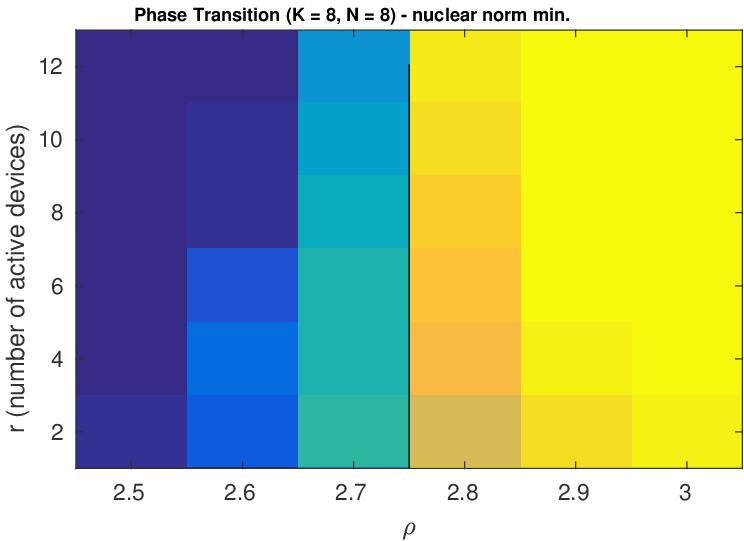
(a)

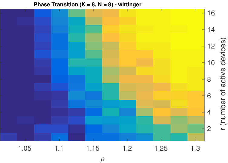
(b)

Figure 1: Phase transition of the success rates per device for (a) the convex approach (1.5) and (b) the Wirtinger approach for $K=N=8$ where $\rho=L/\sum_{i=1}^{r}(K_{i}+N_{i})$.

Appendix A Construction of the partition $\left\{\Gamma_{p}\right\}_{p\in\left[P\right]}$

A.1 Proof of Lemma 2.2

The goal of this section is to prove Lemma 2.2. Our proof will rely on the following lemma.

Lemma A.1.

Fix $i\in\left[r\right]$ and let $Q\in\left(0,L\right)$, $\delta>0$ and $\nu\in\left(0,1\right)$. Assume that

$$Q\geq C\frac{K_{i,\mu}}{\nu^{2}}\log\frac{K_{i}}{\delta},$$ (A.1)

where $C>0$ is an absolute constant and let $\hat{\delta}_{1},\ldots,\hat{\delta}_{L}$ be independent, identically distributed random variables such that

$$\mathbb{P}\left(\hat{\delta}_{1}=1\right)=\frac{Q}{L}\quad\text{and}\quad\mathbb{P}\left(\hat{\delta}_{1}=0\right)=1-\frac{Q}{L}.$$

Then with probability exceeding $1-\delta$ we have that

$$\Big{\|}\frac{L}{Q}\sum_{\ell=1}^{L}\hat{\delta}_{\ell}b_{i,\ell}b^{*}_{i,\ell}-\text{Id}\Big{\|}_{2\rightarrow 2}\leq\nu.$$

A proof of this lemma can be obtained using arguments contained in the proof of Theorem 1.2 in [CR07]. For the sake of completeness we will give a proof below (relying on different techniques). Our proof of Lemma 2.2 will use essentially the same ideas as in [ARR14], but has been slightly refined.

Proof of Lemma 2.2.

Let $\hat{\delta}_{1},\ldots,\hat{\delta}_{k}$ be independent, uniformly distributed random variables which take values in $[P]$. For $p\in[P]$ we define

$$\Gamma_{p}=\left\{\ell\in[L]:\ \hat{\delta}_{\ell}=p\right\}.$$

Thus, $\left\{\Gamma_{p}\right\}_{p\in[P]}$ is a partition of $[L]$. To finish the proof it is enough to show that with positive probability the partition $\left\{\Gamma_{p}\right\}_{p\in[P]}$ has the required properties, i.e., for all $p\in\left[P\right]$, (2.5) holds and $\frac{1}{2}Q\leq|\Gamma_{p}|\leq\frac{3}{2}Q$ . For $i\in[r]$ and $p\in[P]$ we define the event

$$A_{i,p}=\left\{(\ref{partitionequation})\text{ fails}\right\}=\left\{\Big{\|}\frac{L}{Q}\sum_{\ell\in\Gamma_{p}}b_{i,\ell}b^{*}_{i,\ell}-\text{Id}\Big{\|}_{2\rightarrow 2}>\nu\right\}.$$

Set $\delta=\frac{1}{3rP}$ and note that $\log(\frac{K}{\delta})=\log\left(3rPK\right)\lesssim\log\left(\max\left\{r;P;K\right\}\right)$. Thus, by Lemma A.1 we get that $\mathbb{P}\left(A_{i,p}\right)\leq\frac{1}{3rP}$, if the constant in inequality (2.6) is chosen large enough. By a union bound over all choices of $i$ and $p$, (2.5) follows with probability at least $\frac{1}{3}$. It remains to control the size of the sets $\{\Gamma_{p}\}_{p\in[P]}$. By the Bernstein inequality for bounded random variables (e.g., [FR13, Corollary 7.31]) we obtain that for fixed $p\in[P]$ one has $\frac{Q}{2}\leq|\Gamma_{p}|\leq\frac{3Q}{2}$ with probability at least $1-2\exp\left(\frac{-Q}{10}\right)\geq 1-\frac{1}{2P}$, where the last inequality follows from (2.6), if the constant $C$ is chosen large enough. Thus, by a another union bound we observe

$$\mathbb{P}\left(\frac{Q}{2}\leq|\Gamma_{p}|\leq\frac{3Q}{2}\text{ for all }p\in[P]\right)>\frac{1}{2}.$$

Thus with positive probability the partition $\left\{\Gamma_{p}\right\}_{p\in[P]}$ has the required properties. In particular, this implies the existence of a partition $\left\{\Gamma_{p}\right\}_{p\in[P]}$ with the properties stated in Lemma 2.2.

∎

A.2 Proof of Lemma A.1

As already mentioned before this lemma can be proven using arguments from the proof Theorem 1.2 in [CR07]. The arguments in this article are based on Talagrand’s inequality [Tal96] and Rudelson’s Lemma [Rud99]. Recent technical advances (see [Tro15a]) allow us to give a simplified proof.

Proof.

The goal is to use the matrix Bernstein inequality to estimate the spectral norm of

$$Y=\frac{L}{Q}\sum_{\ell=1}^{L}\hat{\delta}_{\ell}b_{i,\ell}b^{*}_{i,\ell}-\text{Id}.$$

We will decompose $Y$ into a sum of independent random matrices with mean zero. Thus, by setting

$$Y_{\ell}=\left(\hat{\delta}_{\ell}-\frac{Q}{L}\right)\frac{L}{Q}b_{i,\ell}b^{*}_{i,\ell}$$

we obtain $Y=\sum_{\ell=1}^{L}Y_{\ell}$ and $\mathbb{E}Y_{\ell}=0$ for all $\ell\in[L]$ due to $\text{Id}=\sum_{\ell=1}^{L}b_{i,\ell}b^{*}_{i,\ell}$. To apply the matrix Bernstein inequality we need first to obtain an upper bound for $\|\mathbb{E}Y^{2}\|_{2\rightarrow 2}$. For that purpose note that

$$\mathbb{E}Y^{2}=\sum_{\ell=1}^{L}\mathbb{E}Y^{2}_{\ell}=\sum_{\ell=1}^{L}\mathbb{E}\left[\left(\hat{\delta}_{\ell}-\frac{Q}{L}\right)^{2}\right]\frac{L^{2}}{Q^{2}}\|b_{i,\ell}\|^{2}_{\ell_{2}}b_{i,\ell}b^{*}_{i,\ell}$$

Observe that $\mathbb{E}\left[\left(\hat{\delta}_{\ell}-\frac{Q}{L}\right)^{2}\right]=\frac{Q\left(L-Q\right)}{L^{2}}$, which implies

$$\mathbb{E}Y^{2}=\frac{L-Q}{L}\sum_{\ell=1}^{L}\frac{L\|b_{i,\ell}\|^{2}_{\ell_{2}}}{Q}b_{i,\ell}b^{*}_{i,\ell}$$

Thus, by $\sum_{\ell=1}^{L}b_{i,\ell}b^{*}_{i,\ell}=\text{Id}$ and the definition of $K_{i,\mu}$ we get

$$\|\mathbb{E}Y^{2}\|_{2\rightarrow 2}\leq\frac{L-Q}{L}\left(\underset{\ell\in[L]}{\max}~{}L\|b_{i,\ell}\|^{2}_{\ell_{2}}\right)\Big{\|}\sum_{\ell=1}^{L}b_{i,\ell}b^{*}_{i,\ell}\Big{\|}_{2\rightarrow 2}\leq\frac{K_{i,\mu}}{Q}.$$

Furthermore, for all $\ell\in[L]$ we have

$$\|Y_{\ell}\|_{2\rightarrow 2}\leq\max\left\{\frac{Q}{L};\frac{L-Q}{L}\right\}\frac{L}{Q}\|b_{i,\ell}\|^{2}_{\ell_{2}}\leq\frac{L}{Q}\|b_{i,\ell}\|^{2}_{\ell_{2}}\leq\frac{K_{i,\mu}}{Q}\quad\text{almost surely.}$$

Thus, we can apply the matrix Bernstein inequality in the version of [Tro15a, Theorem 6.6.1] to obtain

$$\mathbb{P}\left(\|Y\|_{2\rightarrow 2}\geq\nu\right) \leq K\exp\left(\frac{-\nu^{2}/2}{\left(1+\frac{\nu}{3}\right)K_{i,\mu}/Q}\right)\overset{(\ref{onepartition})}{\leq}K\exp\left(\frac{-C\log\left(K/\delta\right)}{2\left(1+\frac{\nu}{3}\right)}\right).$$

As we have $0<\nu<1$ this yields the claim if the constant $C>0$ in (A.1) is chosen large enough.

∎

Appendix B Circular-symmetric Complex Normal Random Variables

In this section we will recall some useful facts concerning random variables which have a circular–symmetric complex normal distribution $\mathcal{CN}(0,\sigma^{2})$ with zero mean and variance $\sigma^{2}$. This means that their real and imaginary parts are uncorrelated jointly Gaussian with zero mean and variance $\sigma^{2}/2$ (and are therefore independent). For more details concerning this probability distribution we refer to [TV05, Section A.1.3]. The following two well-known lemmas are concerned with two useful identities. A proof of them can be found for example in [ARR14, Lemma 11 and 12].

Lemma B.1.

Assume that $c\in\mathbb{C}^{n}$ is a random vector with independent entries $c_{i}\sim\mathcal{CN}(0,1)$. Then we have

$$\mathbb{E}\left[\left(\text{Id}-cc^{*}\right)^{2}\right]=n\text{Id}.$$

Lemma B.2.

Let $q\in\mathbb{C}^{n}$ be any deterministic vector. Furthermore, assume that $c\in\mathbb{C}^{n}$ is a random vector with independent entries $c_{i}\sim\mathcal{CN}(0,1)$. Then we have

$$\mathbb{E}\left[\left(cc^{*}-\text{Id}\right)qq^{*}\left(cc^{*}-\text{Id}\right)\right] =\|q\|^{2}_{\ell_{2}}\text{Id}.$$

The following lemma summarizes well-known facts regarding the tail decay of certain quantities which involve circular-symmetric normal random variables. For the sake of completeness we include a proof.

Lemma B.3.

Suppose that $c\in\mathbb{C}^{N}$ is a random vector with independent entries $c_{i}\sim\mathcal{CN}(0,1)$. Let $p,q\in\mathbb{C}^{N}$ be arbitrary. Then we have the following inequalities:

$$\Big{\|}\|c\|_{\ell_{2}}\Big{\|}_{\psi_{2}} \lesssim\sqrt{N}$$ (B.1)

$$\Big{\|}|c^{*}q|\Big{\|}_{\psi_{2}} \lesssim\|q\|_{\ell_{2}}$$ (B.2)

$$\Big{\|}\|\left(cc^{*}-\text{Id}\right)q\|_{\ell_{2}}\Big{\|}_{\psi_{1}} \lesssim\sqrt{N}\|q\|_{\ell_{2}}$$ (B.3)

$$\Big{\|}p^{*}\left(cc^{*}-\text{Id}\right)q\Big{\|}_{\psi_{1}} \lesssim\|p\|_{\ell_{2}}\|q\|_{\ell_{2}}$$ (B.4)

Proof.

In order to prove (B.1) note that

$$\Big{\|}\|c\|_{\ell_{2}}\Big{\|}^{2}_{\psi_{2}}\lesssim\Big{\|}\|c\|^{2}_{\ell_{2}}\Big{\|}_{\psi_{1}}\leq\sum_{i=1}^{N}\Big{\|}|c_{i}|^{2}\Big{\|}_{\psi_{1}}\lesssim N.$$

The first inequality follows from [Ver12, Lemma 5.14] and for the second one we used the triangle inequality. In order to prove (B.2) it is enough to note that $c^{*}q\sim\mathcal{CN}\left(0,\|q\|^{2}_{\ell_{2}}\right)$. (B.3) follows from the inequality chain

$$\Big{\|}\|\left(cc^{*}-\text{Id}\right)q\|_{\ell_{2}}\Big{\|}_{\psi_{1}} \leq\Big{\|}\|c\|_{\ell_{2}}|c^{*}q|+\|q\|_{\ell_{2}}\Big{\|}_{\psi_{1}}\leq\Big{\|}\|c\|_{\ell_{2}}\Big{\|}_{\psi_{2}}\Big{\|}|c^{*}q|\Big{\|}_{\psi_{2}}+\Big{\|}\|q\|_{\ell_{2}}\Big{\|}_{\psi_{1}}$$

$$\lesssim\sqrt{N}\|q\|_{\ell_{2}}+\|q\|_{\ell_{2}}\lesssim\sqrt{N}\|q\|_{\ell_{2}}.$$

In the second inequality we have used the Hoelder inequality (3.1) and the second line follows directly from (B.1) and (B.2). In a similar way one proves (B.4). ∎

We will also need the following standard fact, which follows from a union bound.

Lemma B.4.

Let $\omega,L\geq 1$ and $\Gamma$ a finite set. For all $i\in[r]$ let $m_{i}\in\mathbb{C}^{N_{i}}$ such that $\|m_{i}\|_{\ell_{2}}=1$. Furthermore, assume that $c_{i,j}\in\mathbb{C}^{N_{i}}$, $i\in[r]$, $j\in\Gamma$, are independent random vectors with i.i.d. entries distributed according to $\mathcal{CN}\left(0,1\right)$. Then with probability at least $1-\mathcal{O}\left(L^{-\omega}\right)$ one has

$$\underset{i\in[r],j\in\Gamma}{\max}\|c_{i,j}\|_{\ell_{2}} \lesssim_{\omega}\max\left\{\sqrt{N\log\left(r|\Gamma|\right)};\ \sqrt{N\log L}\right\}$$

$$\underset{i\in[r],j\in\Gamma}{\max}|c^{*}_{i,j}m_{i}| \lesssim_{\omega}\max\left\{\sqrt{\log\left(r|\Gamma|\right)};\sqrt{\log L}\right\}.$$

We conclude this section with a proof of Corollary 3.4.

Proof of Corollary 3.4.

Observe that

$$\big{\|}Z\big{\|}_{2\rightarrow 2}\leq\big{\|}\sum_{i=1}^{n}\text{Re}\left(\gamma_{i}\right)X_{i}\big{\|}_{2\rightarrow 2}+\big{\|}\sum_{i=1}^{n}\text{Im}\left(\gamma_{i}\right)X_{i}\big{\|}_{2\rightarrow 2}.$$

By Theorem [Tro15b, Theorem 4.1.1] we obtain that with probability at least $1-\exp\left(-t\right)$

$$\big{\|}\sum_{i=1}^{n}\text{Re}\left(\gamma_{i}\right)X_{i}\big{\|}_{2\rightarrow 2}\leq\frac{1}{\sqrt{2}}\sigma\sqrt{t+\log\left(d_{1}+d_{2}\right)}$$

and with probability at least $1-\exp\left(-t\right)$

$$\big{\|}\sum_{i=1}^{n}\text{Im}\left(\gamma_{i}\right)X_{i}\big{\|}_{2\rightarrow 2}\leq\frac{1}{\sqrt{2}}\sigma\sqrt{t+\log\left(d_{1}+d_{2}\right)}.$$

Combining these facts yields the result. ∎

Appendix C Proof of Lemma 5.9

For $i\in[r]$ let $\mathcal{N}_{i}$ be an $\frac{\varepsilon}{2}$-cover of $B\left(0,1\right)\subset\mathbb{C}^{K_{i}}$ with respect to the ${\|\cdot\|_{B_{i}}}$-norm. Furthermore, let $\mathcal{O}$ be an $\frac{\varepsilon}{2\sqrt{K_{\mu}}}$-cover of $B\left(0,1\right)\subset\mathbb{R}^{r}$ with respect to the $\|\cdot\|_{\ell_{2}}$-norm. We will show that any $Z=\left(u_{1}m_{1}^{*},\ldots,u_{r}m_{r}^{*}\right)\in B^{m}$ can be approximated by $Y=\left(\sigma_{1}y_{1}m_{1}^{*},\ldots,\sigma_{r}y_{r}m^{*}_{r}\right)$, where $\sigma=\left(\sigma_{1},\ldots,\sigma_{r}\right)\in\mathcal{O}$ and $y_{i}\in\mathcal{N}_{i}$. This proves the claim, as the number of such $Y$’s is bounded by the right-hand side. For that choose $\sigma=\left(\sigma_{1},\ldots,\sigma_{r}\right)\in\mathcal{O}$ such that

$$\sqrt{\sum_{i=1}^{r}\left(\|u_{i}\|_{\ell_{2}}-\sigma_{i}\right)^{2}}\leq\frac{\varepsilon}{2\sqrt{K_{\mu}}}$$ (C.1)

and $y_{i}\in\mathcal{N}_{i}$ such that

$${\Big{\|}\frac{1}{\|u_{i}\|_{\ell_{2}}}u_{i}-y_{i}\Big{\|}_{B_{i}}}\leq\frac{\varepsilon}{2}.$$ (C.2)

Then one has for $\hat{Y}=\left(\|u_{1}\|_{\ell_{2}}y_{1}m^{*}_{1},\ldots,\|u_{r}\|_{\ell_{2}}y_{r}m^{*}_{r}\right)$

$$\Big{\|}Z-\hat{Y}\Big{\|}^{2}_{B} \leq\sum_{i=1}^{r}\Big{\|}u_{i}m_{i}^{*}-\|u_{i}\|_{\ell_{2}}y_{i}m^{*}_{i}\Big{\|}^{2}_{B_{i}}=\sum_{i=1}^{r}\Big{\|}u_{i}-\|u_{i}\|_{\ell_{2}}y_{i}\Big{\|}^{2}_{B_{i}}$$

$$\leq\frac{\varepsilon^{2}}{4}\sum_{i=1}^{r}\|u_{i}\|_{\ell_{2}}^{2}=\frac{\varepsilon^{2}}{4}\|Z\|^{2}_{F}\leq\frac{\varepsilon^{2}}{4}.$$

The first inequality follows from (5.12) and the next equality follows from

$$\|m_{i}\left(u_{i}-\|u_{i}\|_{\ell_{2}}y_{i}\right)^{*}b_{i,\ell}\|_{\ell_{2}}=|\left(u_{i}-\|u_{i}\|_{\ell_{2}}y_{i}\right)^{*}b_{i,\ell}|$$

which is due to $\|m_{i}\|_{\ell_{2}}=1$. The subsequent inequality is a consequence of (C.2). The second equality again follows from $\|m_{i}\|_{\ell_{2}}=1$ for all $i\in[r]$. Similarly,

$$\|\hat{Y}-Y\|_{B} \leq\sqrt{\sum_{i=1}^{r}\Big{\|}\left(\|u_{i}\|_{\ell_{2}}-\sigma_{i}\right)y_{i}m^{*}_{i}\Big{\|}^{2}_{B_{i}}}=\sqrt{\sum_{i=1}^{r}\left(\|u_{i}\|_{\ell_{2}}-\sigma_{i}\right)^{2}\|y_{i}\|_{B_{i}}^{2}}$$

$$\leq\sqrt{K_{\mu}\sum_{i=1}^{r}\left(\|u_{i}\|_{\ell_{2}}-\sigma_{i}\right)^{2}}\leq\frac{\varepsilon}{2}.$$

Here the second inequality follows from

$${\|y_{i}\|_{B_{i}}}=\sqrt{L}\ \underset{\ell\in[L]}{\max}\ |y^{*}_{i}b_{i,\ell}|\leq\sqrt{L}\|y_{i}\|_{\ell_{2}}\underset{\ell\in[L]}{\max}\|b_{i,\ell}\|_{\ell_{2}}\leq\sqrt{K_{\mu}}$$

and the last inequality is a consequence of (C.1). Combining the two inequalities gives $\|Z-Y\|_{B}\leq\varepsilon$ which finishes the proof. ∎

References

• [AF13] M. S. C. Almeida and M. A. T. Figueiredo, Blind image deblurring with unknown boundaries using the alternating direction method of multipliers, 20th IEEE International Conference on Image Processing, 2013, pp. 586–590.
• [ALMT14] D. Amelunxen, M. Lotz, M. B. McCoy, and J. A. Tropp, Living on the edge: Phase transitions in convex programs with random data, Inf. Inference (2014).
• [AMS04] S. Artstein, V. Milman, and S. J. Szarek, Duality of metric entropy., Ann. of Math. (2) 159 (2004), no. 3, 1313–1328.
• [ARR14] A. Ahmed, B. Recht, and J. Romberg, Blind Deconvolution using Convex Programming, IEEE Trans. Inform. Theory 60 (2014), no. 3, 1711–1732.
• [AW02] R. Ahlswede and A. Winter, Strong converse for identification via quantum channels, IEEE Trans. Inform. Theory 48 (2002), no. 3, 569–579.
• [BCEB08] B. G. Bodmann, P. G. Casazza, D. Edidin, and R. Balan, Frames for linear reconstruction without phase, 42nd Annual Conference on Information Sciences and Systems, 2008, IEEE, 2008, pp. 721–726.
• [Bha96] R. Bhatia, Matrix analysis., New York, NY: Springer, 1996.
• [BN07] L. Balzano and R. Nowak, Blind calibration of sensor networks, Proceedings of the 6th international conference on Information processing in sensor networks, ACM, 2007, pp. 79–88.
• [Car85] B. Carl, Inequalities of Bernstein-Jackson-type and the degree of compactness of operators in Banach spaces, Ann. Inst. Fourier (Grenoble) 35 (1985), no. 3, 79–118.
• [CG84] A. L. Chistov and D. Y. Grigor’ev, Complexity of quantifier elimination in the theory of algebraically closed fields, International Symposium on Mathematical Foundations of Computer Science, Springer, 1984, pp. 17–31.
• [CM14a] S. Choudhary and U. Mitra, Fundamental limits of blind deconvolution Part I: Ambiguity kernel, arXiv preprint arXiv:1411.3810 (2014).
• [CM14b]  , Identifiability scaling laws in bilinear inverse problems, arXiv preprint arXiv:1402.2637 (2014).
• [CM15]  , Fundamental Limits of Blind Deconvolution Part II: Sparsity-Ambiguity Trade-offs, arXiv preprint arXiv:1503.03184 (2015).
• [CP11] E. J. Candès and Y. Plan, Tight oracle inequalities for low-rank matrix recovery from a minimal number of noisy random measurements, IEEE Trans. Inform. Theory 57 (2011), no. 4, 2342–2359.
• [CR07] E. J. Candès and J. Romberg, Sparsity and incoherence in compressive sampling, Inverse problems 23 (2007), no. 3, 969.
• [CRT06] E. J. Candès, J. Romberg, and T. Tao, Robust uncertainty principles: Exact signal reconstruction from highly incomplete frequency information, IEEE Trans. Inform. Theory 52 (2006), no. 2, 489–509.
• [CS11] Y. Chi and L.L. Scharf, Sensitivity to basis mismatch in compressed sensing, IEEE Trans. Signal Process. 59 (2011), no. 5.
• [CSPW09] V. Chandrasekaran, S. Sanghavi, P. A. Parrilo, and A. S. Willsky, Sparse and low-rank matrix decompositions, IFAC Proceedings Volumes (IFAC-PapersOnline), vol. 15, 2009, pp. 1493–1498.
• [CW00] T. F. Chan and C. K. Wong, Convergence of the alternating minimization algorithm for blind deconvolution, Linear Algebra Appl. 316 (2000), no. 1-3, 259–285.
• [DH01] D. L. Donoho and X. Huo, Uncertainty principles and ideal atomic decomposition, IEEE Trans. Inform. Theory 47 (2001), no. 7, 2845–2862.
• [Don06] D. L. Donoho, Compressed sensing, IEEE Trans. Inform. Theory 52 (2006), no. 4, 1289–1306.
• [Dud67] R. M. Dudley, The sizes of compact subsets of hilbert space and continuity of gaussian processes, J. Funct. Anal. 1 (1967), no. 3, 290 – 330.
• [Fliar] A. Flinth, Sparse blind deconvolution and demixing through $\ell_{1,2}$-minimization, Adv. Comput. Math. (to appear).
• [FR13] S. Foucart and H. Rauhut, A Mathematical Introduction to Compressive Sensing, New York, NY: Birkhäuser/Springer, 2013.
• [GE11] S. Gleichman and Y.C. Eldar, Blind compressed sensing, IEEE Trans. Inform. Theory 57 (2011), no. 10, 6958–6975.
• [God80] G. H. Godard, Self-recovering equalization and carrier tracking in two dimensional data communication systems, IEEE Trans. Commun. 28 (1980), no. 11, 1867–1875.
• [Gro11] D. Gross, Recovering low-rank matrices from few coefficients in any basis, IEEE Trans. Inform. Theory 57 (2011), no. 3, 1548–1566.
• [Hay94] S. Haykin, Blind Deconvolution, Prentice Hall, New Jersey, 1994.
• [HS10] M.A. Herman and T. Strohmer, General deviants: An analysis of perturbations in compressed sensing, IEEE J. Sel. Topics Signal Process. 4 (2010), no. 2.
• [JW15] P. Jung and P. Walk, Sparse Model Uncertainties in Compressed Sensing with Application to Convolutions and Sporadic Communication, Compressed Sensing and its Applications (Holger Boche, Robert Calderbank, Gitta Kutyniok, and Jan Vybiral, eds.), Springer, 2015, pp. 1–29.
• [KJ16] R. Kueng and P. Jung, Robust Nonnegative Sparse Recovery and 0/1-Bernoulli Measurements, IEEE Inf. Theory Workshop (ITW), 2016.
• [KK17] M. Kech and F. Krahmer, Optimal injectivity conditions for bilinear inverse problems with applications to identifiability of deconvolution problems, SIAM J. Appl. Algebra Geom. 1 (2017), no. 1, 20–37.
• [KMR14] F. Krahmer, S. Mendelson, and H. Rauhut, Suprema of chaos processes and the restricted isometry property., Comm. Pure Appl. Math. 67 (2014), no. 11, 1877–1904.
• [Kol13] V. Koltchinskii, A remark on low rank matrix recovery and noncommutative bernstein type inequalities, Collections, vol. Volume 9, pp. 213–226, Institute of Mathematical Statistics, Beachwood, Ohio, USA, 2013.
• [KR61] M. A. Krasnosel’skii and Y.B. Rutickii, Convex functions and Orlicz spaces, Noordhoff, Gröningen (1961).
• [KW14] F. Krahmer and R. Ward, Stable and robust sampling strategies for compressive imaging, IEEE Trans. Image Process., vol. 23, 2014, pp. 612–622.
• [LJ15] K. Lee and M. Junge, RIP-like Properties in Subsampled Blind Deconvolution, arXiv preprint arXiv:1511.06146 (2015).
• [LLB15] Y. Li, K. Lee, and Y. Bresler, A Unified Framework for Identifiability Analysis in Bilinear Inverse Problems with Applications to Subspace and Sparsity Models, arXiv preprint arXiv:1501.06120 (2015).
• [LLB17]  , Identifiability and stability in blind deconvolution under minimal assumptions, IEEE Trans. Inform. Theory (2017).
• [LLJB17] K. Lee, Y. Li, M. Junge, and Y. Bresler, Blind recovery of sparse signals from subsampled convolution, IEEE Trans. Inform. Theory 63 (2017), no. 2, 802–821.
• [LLSW16] X. Li, S. Ling, T. Strohmer, and K. Wei, Rapid, Robust, and Reliable Blind Deconvolution via Nonconvex Optimization, arXiv 1606.04933 (2016), 1–49.
• [LS15a] S. Ling and T. Strohmer, Blind Deconvolution Meets Blind Demixing: Algorithms and Performance Bounds, arXiv:1512.07730 (2015).
• [LS15b] S. Ling and T. Strohmer, Self-calibration and biconvex compressive sensing, Inverse Problems 31 (2015), no. 11.
• [LS17]  , Regularized Gradient Descent: A Nonconvex Recipe for Fast Joint Blind Deconvolution and Demixing, arXiv preprint arXiv:1703.08642 (2017).
• [LWB13] K. Lee, Y. Wu, and Y. Bresler, Near optimal compressed sensing of a class of sparse low-rank matrices via sparse power factorization, arXiv preprint arXiv:1312.0525 (2013).
• [LWDF] A. Levin, Y. Weiss, F. Durand, and W. T. Freeman, Understanding and evaluating blind deconvolution algorithms, IEEE Conference on Computer Vision and Pattern Recognition, 2009, pp. 1964–1971.
• [MT14] M. B. McCoy and J. A. Tropp, Sharp recovery bounds for convex demixing, with applications, Found. Comput. Math. 14 (2014), no. 3, 503–567.
• [MT17]  , The achievable performance of convex demixing, ACM Technical Report 2017-02, California Institute of Technology, 2017.
• [OJF+15] S. Oymak, A. Jalali, M. Fazel, Y. C. Eldar, and B. Hassibi, Simultaneously Structured Models with Application to Sparse and Low-rank Matrices, IEEE Trans. Inform. Theory 61 (2015), no. 5.
• [Pie72] A. Pietsch, Theorie der Operatorenideale, Wissenschaftliche Beiträge der Friedrich-Schiller-Universität Jena, Friedrich-Schiller-Universität Jena, Jena, 1972.
• [RFP10] B. Recht, M. Fazel, and P. A. Parrilo, Guaranteed minimum-rank solutions of linear matrix equations via nuclear norm minimization., SIAM Rev. 52 (2010), no. 3, 471–501.
• [ROV14] E. Richard, G. Obozinski, and J.P. Vert, Tight convex relaxations for sparse matrix factorization, arXiv preprint arXiv:1407.5158 (2014), 1–52.
• [RSS17] H. Rauhut, R. Schneider, and Ž. Stojanac, Low rank tensor recovery via iterative hard thresholding, Linear Algebra Appl. 523 (2017), 220–262.
• [Rud99] M. Rudelson, Random vectors in the isotropic position., J. Funct. Anal. 164 (1999), no. 1, 60–72.
• [SCI75] T. G. Stockham, T. M. Cannon, and R. B. Ingebretsen, Blind deconvolution through digital signal processing, Proc. IEEE 63 (1975), no. 4, 678–692.
• [SJK16] D. Stöger, P. Jung, and F. Krahmer, Blind deconvolution and Compressed Sensing, Cosera 2016, 2016.
• [SJK17]  , Blind Demixing and Deconvolution with Noisy Data: Near-optimal Rate, 21st International ITG Workshop on Smart Antenna, 2017.
• [Tal96] M. Talagrand, New concentration inequalities in product spaces, Invent. Math. 126 (1996), no. 3, 505–563.
• [Tal14]  , Upper and lower bounds for stochastic processes: modern methods and classical problems, 2014.
• [Tro12] J. A. Tropp, User-friendly tail bounds for sums of random matrices, Found. Comput. Math. 12 (2012), no. 4, 389–434.
• [Tro15a] J. A. Tropp, An introduction to matrix concentration inequalities., Found. Trends Mach. Learn. 8 (2015), no. 1-2, 1–230.
• [Tro15b] J. A. Tropp, Sampling theory, a renaissance: Compressive sensing and other developments, ch. Convex Recovery of a Structured Signal from Independent Random Linear Measurements, pp. 67–101, Springer International Publishing, 2015.
• [TV05] D. Tse and P. Viswanath, Fundamentals of Wireless Communication, Cambridge University Press, New York, NY, USA, 2005.
• [Ver12] R. Vershynin, Introduction to the non-asymptotic analysis of random matrices, Compressed Sensing (Y. C. Eldar and G. Kutyniok, eds.), Cambridge University Press, 2012, Cambridge Books Online, pp. 210–268.
• [WBSJ15] G. Wunder, H. Boche, T. Strohmer, and P. Jung, Sparse Signal Processing Concepts for Efficient 5G System Design, IEEE Access 3 (2015), 195–208.
• [WGMM13] J. Wright, A. Ganesh, K. Min, and Y. Ma, Compressive principal component pursuit, Inf. Inference 2 (2013), no. 1, 32–68.
• [WJPH16] P. Walk, P. Jung, G. E. Pfander, and B. Hassibi, Ambiguities of Convolutions with Application to Phase Retrieval Problems, Asilomar 2016, invited paper, 2016.
• [WP98] X. Wang and H. V. Poor, Blind equalization and multiuser detection in dispersive CDMA channels, IEEE Trans. Commun. 46 (1998), no. 1, 91–103.