A symmetry-adapted numerical scheme for SDEs
Abstract
We propose a geometric numerical analysis of SDEs admitting Lie symmetries which allows us to individuate a symmetry adapted coordinates system where the given SDE has notable invariant properties. An approximation scheme preserving the symmetry properties of the equation is introduced. Our algorithmic procedure is applied to the family of general linear SDEs for which two theoretical estimates of the numerical forward error are established.
1 Introduction
The exploitation of special geometric structures in numerical integration of both ordinary and partial differential equations
(ODEs and PDEs) is nowadays a mature subject of the numerical analysis often called geometric numerical integration
(see e.g. [17, 24, 28, 38]). The importance of this research topic is due to the
fact that many differential equations in mathematical applications have some particular geometrical features such as for
example a conservation law, a variational origin, an Hamiltonian or symplectic structure, a symmetry structure etc.. The
development of geometrically adapted numerical algorithms permits to obtain suitable integration methods which both preserve
the qualitative properties of the integrated equations and have a more efficient numerical behaviour with respect to the
corresponding standard discretization schemes.
In comparison the study of geometric numerical integration of stochastic differential equations (SDEs) is not so well developed.
In the current literature the principal aims consist in producing numerical stochastic integrators which are able to preserve the
symplectic structure (see e.g. [1, 35, 40]), some conserved quantities (see e.g. [5, 23, 32])
or the variational structure (see e.g. [2, 3, 22, 42]) of the considered SDEs. For the study of the algebraic structure of stochastic expansions in order to achive an optimal efficient stochastic integrators at all
orders see [11].
Although the exploitation of Lie symmetries of ODEs and PDEs (see e.g. [36]) to obtain better numerical integrators
is an active research topic (see e.g. [4, 10, 31, 30] and references therein), the
application of the same techniques in the stochastic setting to the best of our knowledge is not yet pursued, probably because
the concept of symmetry of a SDE has been quite recently developed (see e.g. [6, 9, 8, 7, 16, 27, 29, 33]).
In this paper we introduce two different numerical methods taking advantage of the presence of Lie symmetries in a given SDE in order to provide a more efficient numerical integration of it.
We first propose the definition of an invariant numerical integrator for a symmetric SDE as a natural generalization of the
corresponding concept for an ODE. When one tries to construct general invariant numerical methods in the stochastic framework,
in fact, a non trivial problem arises. Since both the SDE solution as well as the Brownian motion driving it are continuous
but not differentiable processes, the finite differences discretization could not converge to the SDE solution. We give some necessary and sufficient conditions in order that the two standard numerical methods for SDEs (the Euler and the Milstein schemes) are also invariant numerical methods. By using this result, in particular, we are able to identify a class of privileged coordinates systems where it is convenient to make the discretization procedure.
Our second numerical method, based on a well-defined change of the coordinates system, is inspired by the standard techniques
of reduction and reconstruction of a SDE with a solvable Lie algebra of symmetries (see [8, 26]). Indeed a SDE
with a solvable Lie algebra of symmetries can be reduced to a triangular system and, when the number of symmetries is sufficiently
high, the latter can be explicitly integrated. In the stochastic setting the explicit integration concept is of course a quite
different notion with respect to the deterministic one. Indeed the evaluation of an Ito integral, a necessary step in the reconstruction
of a reduced SDE, can only be numerically implemented.
We apply our two proposed numerical techniques to the general linear SDEs, being the first non-trivial class of symmetric
equations. In this case the two algorithmic methods can be harmonized in such a way to produce the same simple family of best coordinates
systems for the discretization procedure. Interestingly, the identified coordinate changes are closely related to the explicit
solution formula of linear SDEs. Although the integration formula of linear SDEs is widely known, it is certainly original the
recognition of the proposed numerical scheme for linear SDEs as a particular implementation of a general procedure for SDEs with Lie symmetries. We finally point out that the simple case of affine drift and diffusion coefficients plays an important role since any SDE with real analytic drift and diffusion coefficients can be seen locally like it.
Moreover we theoretically investigate the numerical advantages of the new numerical scheme for linear SDEs. More precisely we obtain
two estimates for the forward numerical error which, in presence of an equilibrium distribution, guarantee that the constructed method
is numerically stable for any size of the time step . This means that for any the error does not grow exponentially with the
maximum-integration-time , but it remains finite for . This property is not shared by standard explicit or
implicit Euler and Milstein methods. The obtained estimates can be considered original results mainly because the coordinate changes
involved in the formulation of our numerical scheme are strongly not-Lipschitz, and so the standard convergence theorems can not be
applied. Our theoretical results are also numerically illustrated.
It is interesting to note that the main part of the theory, in particular the definitions of strong symmetry of a SDE and of numerical scheme, can be easily extended to Stratonovich type SDE driven by general noises ([6]), for example by exploiting rough paths theory. Unfortunately, since the proofs of Theorem 5.1 and Theorem 5.2 use in essential way the (forward and bachward) Ito formula, the long terms estimates obtained here cannot be straightforwardly generalized to the rough paths driven SDEs framework. At the same time we think that some ideas in the proof of Theorem 5.2 can be suitable exploited to obtain pathwise estimates of long term error in the rough paths setting.
The article is structured as follows: in Section 2 we recall the notion of strong symmetry of a SDE and we
describe the two standard discretization schemes used in the rest of the paper. In Section 3 we propose
two numerical procedures adapted with respect to the Lie symmetries of a SDE. We apply the proposed integration methods to general one and two-dimensional linear SDEs in Section 4 . In Section 5 some theoretical estimates showing the stability
and efficiency of our adapted-to-symmetries numerical schemes in linear-SDEs are proved. In the last section we expose some numerical
experiments confirming the theoretical estimates obtained in the previous section.
2 Preliminaries
2.1 Strong symmetries of SDEs
In the following will be an open subset of , and will be the standard coordinates system of . If we denote by the Jacobian of i.e. the matrix-valued function
Furthermore we can identify the vector fields with the functions , and if is a diffeomorphism (with ) we introduce the pushforward
Definition 2.1
Let be a filtered probability space. Let and be two smooth functions defined on and valued in n vectors and matrices respectively. A solution to a SDE() is a pair of adapted processes such that
i) W is a -Brownian motion in ;
ii) For
| (1) |
Remark 2.2
In particular all the integrals are meaningful if a.s.:
Definition 2.3
A solution to a SDE() on is said a strong solution if is adapted to the filtration generated by the BM and completed with respect to .
Of course a solution is called a weak solution when it is not strong.
In this paper we fix a Brownian motion , that is we consider only strong solutions of a SDE() and, consequently, we denote them simply by . For a symmetry analysis via weak solutions of SDEs see [9].
A solution to a SDE() is a diffusion process admitting as infinitesimal generator:
It is particularly useful for obtaining stochastic differentials the following celebrated formula.
Theorem 2.4 (Ito formula)
Let be a solution of the SDE and let be a smooth function. Then has the following stochastic differential
We recall important definitions of symmetries of a SDE.
Definition 2.5 (strong finite symmetry)
We say that a diffeomorphism is a (strong finite) symmetry of the SDE if for any solution to the SDE also is a solution to the SDE .
By using Ito formula it is immediate to prove the following result.
Theorem 2.6
A diffeomorphism is a symmetry of the SDE if and only if
It is well-known that vector fields acting as infinitesimal generators of one parameter transformation groups are the most important tools in Lie group theory.
Definition 2.7 (strong infinitesimal symmetry)
A vector field is said a (strong infinitesimal) symmetry of the SDE if the group of the local diffeomorphism generated by is a symmetry of the SDE for any .
The following determining equations for (any) infinitesimal symmetries are well-known (see, e.g., [16]). For their generalization to a weak solution case see [9].
Theorem 2.8 (Determining equations)
A vector field is an infinitesimal symmetry of the SDE if and only if
| (2) | |||||
| (3) |
where is the -column of () and are the standard Lie brackets between vector fields.
2.2 Numerical integration of SDEs
For convenience of the reader, we recall the two main numerical methods for simulating a SDE and a theorem on the strong convergence of these methods (for a detailed description see e.g. [25]).
Consider the SDE having coefficients , driven by the Brownian motion , and let be a partition of . The Euler scheme for the equation with respect to the given partition is provided by the following sequence of random variables
where and . The Milstein scheme for the same equation is instead constituted by the sequence of random variables such that
where . We recall that when we have that
Theorem 2.9
Let us denote by the exact solution of a SDE and by and the N-step approximations according with Euler and Milstein scheme respectively. Suppose that the coefficients are with bounded derivatives and put and . Then there exists a constant such that
Furthermore when the coefficients are with bounded derivatives then there exists a constant such that
Proof. See Theorem 10.2.2 and Theorem 10.3.5 in [25].
Theorem 2.9 states that and strongly converge in to the exact solution of the
SDE , where the order of the convergence with respect to the step size variation is in the
Euler case and in the Milstein one.
Nevertheless the theorem gives no information on the behaviour of the numerical approximations when we fix the step size and we vary
the final time . In the standard proof of Theorem 2.9 one estimates the constants and
by proving that there exist two positive constants such that
and , by using Gronwall Lemma. In
some situations the exponential growth of the error is a correct prediction (see for example [34]).
Of course this fact does not mean that in
any case the errors and exponentially diverge with the time . Indeed if the SDE admits an equilibrium distribution it could happen that the two errors remain bounded with
respect to the time . Unfortunately this favorable situation does not happen for any values of the step size , but only for values
within a certain region. The phenomenon just described is known as the stability problem for a discretization method of a SDE.
This problem, and the corresponding definition, is usually stated and tested for some specific SDEs (see e.g. [19, 41]
for the geometric Brownian motion, see e.g. [18, 39] the Ornstein-Uhlenbeck process, see e.g.
[20, 21] for non-linear equations with a Dirac delta equilibrium distribution, and see e.g. [43]
for more general situation). We will show some numerical examples of the stability phenomenon for general linear SDEs in Section
6.
3 Numerical integration via symmetries
3.1 Invariant numerical algorithms
When a system of ODEs admits Lie-point symmetries then invariant numerical algorithms can be constructed (see e.g. [31, 30, 10, 4]). By completeness we recall the definition of an invariant numerical scheme for a system of ODEs, in the simple case of one-step algorithms. The obvious extension for multi-step numerical schemes is immediate. The discretization of an ODEs system is a function such that if are the steps respectively and is the step size of our discretization we have that
If is a diffeomorphism we say that the discretization defined by the map is invariant with respect to the map if it happens that
If we require that the previous property holds for any and for any we get
| (4) |
for any and . If is an one-parameter group generated by the vector field , by deriving the relation with respect to , we obtain the relation
| (5) |
which guarantees that the discretization is invariant with respect to , generated by
.
We can extend the previous definition to the case of a SDE in the following way. Let us discuss an integration scheme which depends only on the time and on the Brownian motion (as for example the Euler method). The same discussion for integration methods depending also on or other random variables (as the Milstein method) is immediate. In the stochastic case the discretization is a map and we have
| (6) | |||||
| (7) |
Since Ito integral strongly depends on the fact that the approximation is backward (and not forward), we stress again that it is not easy to prove that a given discretization converges to the real solution of the SDE . For this reason we give a theorem which provides a sufficient (and necessary) condition in order that Euler and Milstein discretizations of a SDE are invariant with respect to any strong symmetries .
Theorem 3.1
Let be strong symmetries of a SDE . When are polynomials of first degree in , then the Euler discretization (or the Milstein discretization) of the SDE is invariant with respect to . If for a given , , also the converse holds.
Proof. We give the proof for the Euler discretization because for the Milstein discretization the proof is very similar. In the case of Euler discretization we have that
The discretization is invariant if and only if
Recalling that is a symmetry for the SDE and therefore it has to satisfy the determining equations (2) and (3), we have that the Euler discretization is invariant if and only if
| (8) |
Suppose that , then
Conversely, suppose that the Euler discretization is invariant and so equality (8) holds. Let be as in the hypotheses of the theorem and choose . Then
Since are arbitrary and , must be of first degree in .
Remark 3.2
The affinity of the coefficients in Theorem 3.1 strongly depends on the fact that Euler and Milstein numerical approximations depend in an affine way from the noise . If we coonsider a non affine numerical approximation we can have non affine symmetries (see the discussion below).
Theorem 3.1 can be fruitfully applied in the
following way. If are strong symmetries of a SDE we
search a diffeomorphism (i.e. a coordinate change) such that
have coefficients of first degree in
the new coordinates system . We discretize the
transformed SDE using the Euler
discretization, obtaining a discretization which is invariant with respect to
. As a consequence the discretization
is
invariant with respect to . It is easy to prove that if the map is
Lipschitz we have that the constructed discretization converges in
to the solution, while if the map is only locally Lipschitz, the weaker convergence in probability can be established.
The existence of the diffeomorphism allowing the application of
Theorem 3.1 for general is not
guaranteed. Furthermore, even when the map exists, unfortunately in general it is
not unique. Consider for example the following one-dimensional SDE
| (9) |
which has
as a strong symmetry. There are many transformations which are able to put with coefficients of first degree, for example the following two transformations:
Indeed we have that
While the map transforms equation (9) into a geometrical Brownian motion, the transformation reduces equation (9) to a Brownian motion with drift. By applying Euler method by means of we obtain a poor numerical result ( in fact is not a Lipschitz function and in this circumstance errors are amplified). By exploiting to make the discretization we obtain instead an exact simulation. The example shows that this first approach strongly depends on the choice of the diffeomorphism (which has to be invertible in terms of elementary functions). So it is better to have another procedure able to individuate the best coordinate system for performing the SDE discretization.
3.2 Adapted coordinates and triangular systems
We introduce a further possible use of Lie’s symmetries in the numerical simulation of a SDE which turns out to be relevant only in the stochastic framework. Indeed in the deterministic setting one can obtain a completely explicit result.
Suppose that , with standard cartesian coordinates , and consider the following triangular SDE
where do not depend on
. The above SDE is triangular in
the variables . By discretizing a triangular SDE we reasonable aspect a better behavior than in the general case. Furthermore if can be exactly simulated with
growing at most polynomially, we can
conjecture that the error grows polynomially with respect to the maximal integration
time .
We recall that the triangular property of stochastic systems is closely related with their symmetries and in particular to SDEs with a solvable Lie algebra of symmetries. In order to briefly explain the connection between symmetries and the triangular form of SDEs, we introduce the following definitions (for more details see [8]).
Definition 3.3
A set of vector fields on is called regular on if, for any , the vectors are linearly independent.
Definition 3.4
Let be a set of regular vector fields on which are generators of a solvable Lie algebra . We say that are in canonical form if there are such that and
where are smooth functions.
Theorem 3.5
Let a SDE admit as strong symmetries and let us suppose that constitute a solvable Lie algebra in canonical form. Then the SDE assumes a triangular form with respect to .
As a notable consequence when we have a SDE admitting a solvable regular Lie algebra we can apply a methodology similar to the one proposed in the previous subsection. Indeed we can start by searching a map such that constitute a solvable Lie algebra in canonical form so implying that is a triangular SDE. We can discretize according with one of standard methods obtaining a discretization . By composing with we obtain a discretization which, when is Lipschitz, has the property of being a more simple triangular discretization scheme. Differently from Theorem 3.1, in the present situation we can always construct the diffeomorphism , as the following proposition states.
Proposition 3.6
Let be an -dimensional solvable Lie algebra on such that has constant dimension as a distribution of . Then, for any , there exist a set of generators of and a local diffeomorphism , such that are generators in canonical form for .
Proof. See [8].
We conclude by pointing out that for a general solvable Lie algebra , the map , whose existence is guaranteed by Proposition 3.6, does not transform into a set of vector fields with coefficients of first degree in . For this reason and by Theorem 3.1, the discretization constructed by using the diffeomorphism and the usual Euler discretization algorithm is not invariant with respect to .
Nevertheless if we consider solvable Lie algebras satisfying a special relation, then will have coefficients of first degree in .
Proposition 3.7
Suppose that the Lie algebra is such that . Then the coefficients of are of first degree in . Moreover one can choose such that the coefficients of are of first degree in all the variables .
Proof. Let us suppose that generates . Then for . Using the fact that and the fact that are in canonical form, we must have that do not depend on and their coefficients must be of first degree in .
The second part of the proposition follows from the well known fact that when the vector fields generate an integrable distribution, it is possible to choose a local coordinate system such that the coefficients of do not depend on .
4 General linear SDEs
We first consider the one-dimensional linear SDE
| (10) |
where and we apply the procedure previously presented
in order to obtain a symmetry adapted discretization scheme.
Although it is possible to prove that equation (10) for does not admit strong symmetries (see [9]), we can look at equation (10) as a part of a two dimensional system admitting Lie symmetries.
Let us consider the system
| (11) |
on , consisting of the original linear equation and the associated homogeneous one. It is simple to prove, by solving the determining equations (2) and (3), that the system (11) admits the following two strong symmetries:
The more general adapted coordinate system system for the symmetries is given by
where and is a smooth function. Indeed in the coordinate system we have that
In order to guarantee that the Euler and Milstein discretization schemes are invariant, by Theorem 3.1 it is sufficient to choose for some constant .
In the new coordinates the original two dimensional SDE becomes
| (16) | |||||
| (17) |
In the following, for simplicity, we consider the discretization scheme only for . The Euler integration scheme becomes:
and the Milstein scheme:
We note that when the
two discretization schemes coincide.
Coming back to the original problem, in the Euler case we get:
| (22) |
and in the Milstein case we obtain:
| (23) |
Remark 4.1
There is a deep connection between equations (22) and (23) and the well-known integration formula for scalar linear SDEs. Indeed the equation (10) admits as solution
| (24) |
where
Equation (22) and (23) can be viewed as the equations obtained by expanding the integrals in formula (24) according with stochastic Taylor’s Theorem (see [25]). This fact should not surprise since the adapted coordinates obtained in Subsection 3.2 were introduced exactly to obtain formula (24) from equation (11). Since the discretizations schemes (22) and (23) are closely linked with the exact solution formula of linear SDEs we call them exact methods (or exact discretizations) for the numerical simulation of linear SDEs.
Let us now consider the following two dimensional SDE
The previous equation can be solved explicitly. In particular the homogeneous linear part has solution given by (see, e.g. [12])
where . Thus the solution of the initial equation is
The Euler discretization of the previous equation becomes:
where and .
5 Theoretical estimation of the numerical forward error for linear SDEs
We provide an explicit estimation of the forward error associated with the exact numerical schemes proposed in the previous section for simulating a
general linear SDE. The explicit solution of a linear SDE is well known and the use of the resolutive formula for its simulation is extensively used, but in the literature, to the best of our knowledge, there is no explicit estimation of the forward error.
5.1 Enunciates of the Theorems
Dividing in parts we obtain instants , with . We denote by the approximate
solution given by exact Euler method, the approximate solution with respect to exact Milstein
method and by the exact solution to the linear SDE. In the following we will omit where it is possible.
Theorem 5.1
For all , we have
where , is a continuous function and is a strictly positive continuous function such that for
| if | ||||
| if | ||||
| if |
with .
Theorem 5.2
For all , we have that
where , is a continuous function and is a strictly positive continuous function such that for
| if | ||||
| if |
with .
Before giving the proof of the two previous theorems we propose some remarks. We recall that a linear SDE with has an equilibrium
distribution if and only if . Furthermore the equilibrium distribution admits a finite first moment if and only if
and a finite second moment if and only if . Since we approximate the Ito integral up to the order ,
the three cases in Theorem 5.1 follow from the fact that for giving an estimate of the error in Euler discretization we need
a second moment control. More precisely we can expect a bounded error with respect to only when the second moment is finite as
.
Since in the Milstein case a finite first moment sufficies, in the second theorem we obtain that the error does not grow with when .
We can obtain an analogous estimate for the Euler method when , i.e. in the case in which the Milstein and Euler discretizations coincide (situation similar to the additive-noise-SDEs setting). The use of only the first moment finitess for estimating the error has a price: indeed we obtain an dependence of the error. We remark that the techniques used in the proof of Theorem 5.2 exploit
some ideas from the recent rough path integration theory (see e.g. [15]), and in particular this circumstance explains
the order of convergence. This fact induces us to conjecture that our proof probably works also in the general rough path framework
(for example for fractional Brownian motion by following [14]). If in Theorem 5.2 we do not require an uniform-in-time
estimate, we can apply the methods used in the proof of Theorem 5.1 for obtaining an error convergence of order .
Essentially the above theorems prove that for and for respectively, our symmetry adapted discretization methods
are stable for any value of . In Section 6 we give a comparison between the stability of the adapted-coordinates
schemes with respect to the standard Euler and Milstein ones, via numerical simulations.
We conclude by noting that Theorem 5.1 and Theorem 5.2 cannot be deduced in a trivial way from the standard theorems
about the convergence of Euler and Milstein methods (such as Theorem 2.9). Indeed the Euler and Milstein discretizations
of equations (16) and (17) do not have Lipschitz coefficients. Furthermore even if a given
discretization of the system composed by (16) and (17) should converge to the exact
solution in , being the coordinate change ( introduced in Section 4) not globally Lipschitz, it
does not imply that the transformed discretization converges to the exact solution of the equation (11)
in . Finally, as pointed out in Subsection 2.2, Theorem 2.9 does not guarantee
an uniform-in-time convergence as Theorem 5.1 and Theorem 5.2 instead state.
For proving the theorems we need the following two lemmas. The second allows to avoid very long calculations (see Appendix A).
Lemma 5.3
Let be a Brownian motion, and then for any
is a continuous function of and in particular it is locally bounded. Moreover we have that
Proof. The proof is based on the fact that is a normal random variable with zero mean and variance equal to .
Lemma 5.4
Let be a smooth function such that and such that
for some , for any and for some continuous function . Then there exists an increasing function such that
If furthermore and
there exists an increasing function such that
Proof. The statements of the lemma derive as special cases from Lemma 5.6.4 and Lemma 5.6.5 in [25].
5.2 Proof of Theorem 5.1
We consider the case . In fact we will find that our estimate is uniform for . Using the notations in Remark 4.1 we can write where
Also the approximation can be written as the sums of two integrals of the form where
Obviously the strong error can be estimated by , where hereafter .
5.2.1 Estimate of
Setting for any , we obtain (with )
By Jensen’s inequality
and by Fubini theorem we have to calculate . Since
and for any we obtain that
| (33) |
because and are independent as a consequence of the Brownian increments
independence.
It is simple to note that the function
satisfies and, by Lemma 5.3,
Thus, by Lemma 5.4, there exists an increasing function
Using Lemma 5.3 we get
obtaining
| (34) |
where
| (35) |
5.2.2 Estimate of
We first consider . Since Ito integral involves adapted processes we cannot bring under the integral sign. However it is possible to take advantage of the backward integral formulation which allows to integrate processes that are measurable with respect to the (future) filtration . In particular when is -measurable then
where is a sequence of points partitions of the interval , having amplitude decreasing to and the limit is understood in probability.
When is a regular function, is a process which is measurable with respect to both the filtrations and ; therefore one can calculate either and .
The next well-known lemma says that we can write in terms of a backward
integral, which allows to bring under the integral sign.
Lemma 5.5
Let be a -function such that
Then
Proof. We report the proof for convenience of the reader (see, e.g., [37]). Setting
since is then also is . From this fact one deduces that
By equating the two expressions one obtains the final formula.
Remark 5.6
Since in the proof of Lemma 5.5 the backward Ito integral plays a fundamental role, the same result cannot be obtained within a pathwise approach such as the rough paths one.
Since
and , by Lemma 5.5, we can write
Introducing and
we have that
| (36) |
We first consider the term . The process can be written as where is the measurable process given by
where is the characteristic function of the interval . By Ito’s isometry and Fubini’s Theorem we obtain
| (37) |
Since Brownian motion has independent increments, we have that
Introducing the function:
which satisfies , by Lemma 5.4 and Lemma 5.3 we obtain
where is an increasing function and, finally,
| (38) |
where
| (39) |
In order to estimate the other term in the right-hand side of (36) we note that by introducing
we have
and
By applying Lemma 5.5 to we can write
From the previous equality, by Ito isometry and Minkowski’s integral inequality we get
where
When , by independence
Introducing
we have that and , , and so, by Lemma 5.4, there exist two continuous increasing functions such that
Since by independence
analogously we can prove that there exists an increasing function such that
For the second term in the right-hand side of (36), we have finally the following estimate
| (40) |
5.3 Proof of Theorem 5.2
We make the proof only for , since in the other case the estimate are equal to the Euler case and can be addressed with the same proof. We introduce the two integrals
5.3.1 Estimate of
First we note that (with )
where we have taken, , and such that (the last condition guarantees that when we have ). By Jensen’s inequality and Lemma 5.4 we can derive the following estimate:
where is an increasing function and in the last inequality we have used the fact that the function is such that . By Lemma 5.3, we have that
and so
where
| (41) |
5.3.2 Estimate of
First we note that
where are as in the previous subsection. We introduce the following notation
where we have used Lemma 5.5 and the fact that . By introducing also and
we have that
It is simple to see that the two norms on the right-hand side of the previous expression do not depend on but only on the difference , so we study the functions (with ):
By a well-known consequence of Ito isometry (see, e.g., [13]) we can estimate the function as:
where . Since the function
satisfies , by Lemma 5.4 there exists an increasing function such that
As far as concerned the function , by introducing
it is immediate to see that
By applying Lemma 5.5 to , and by noting that , we obtain
Since we have that , and that , by Jensen’s inequality, Lemma 5.4 and by applying the same techniques used for obtaining (40) we find that
or, equivalently,
with the obvious definition of the function .
Finally we have
where is given by (41).
6 Numerical examples
We show some numerical experiments which confirm the theoretical estimate proved in Section 5 and permit to study other properties of the new discretization methods introduced in Section 4.
We simulate the linear SDE (10) with coefficients , , e . The coefficients are such that with . This means that the considered linear equation admits an equilibrium probability density with finite first moment and infinite second moment. The coefficient has been chosen big enough to put in evidence the noise effect.
We make a comparison between the Euler and Milstein methods applied directly to equation (10) and the new exact methods (22) and (23) with the constants and . In particular we observe that when , the schemes (22) and (23) coincide. We calculate the following two errors:
-
•
the weak error ,
-
•
the strong error .
The weak error is estimated trought the explicit expression
for the first moment of the linear SDE solution, and by using Monte-Carlo method with paths for calculating . The strong error is estimated by exploiting Monte-Carlo simulation of and with paths. In order to simulate we apply the Milstein method with a steps-size of , for which we have verified that it gives a good approximation of both and the equilibrium density for . Since we use Monte-Carlo methods for estimating and , the two errors include both the systematic errors of the considered schemes and the statistical errors of the Monte-Carlo estimate procedure.


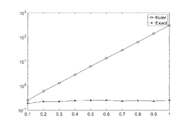
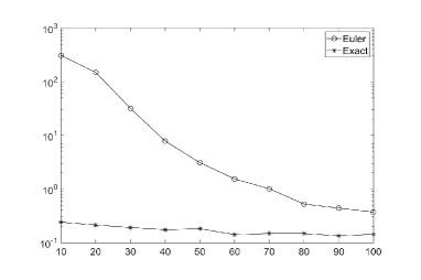
In Figure 1 we report the weak and strong errors with respect to the maximum time of integration which varies from to and stepsize . As predicted by Theorem 5.2, the error of the exact method for remains bounded. It is important to note that for the exact method in the case (where Theorem 5.1 and Theorem 5.2 do not apply) the errors remains bounded too, while for Euler and Milstein methods the errors grow exponentially with .
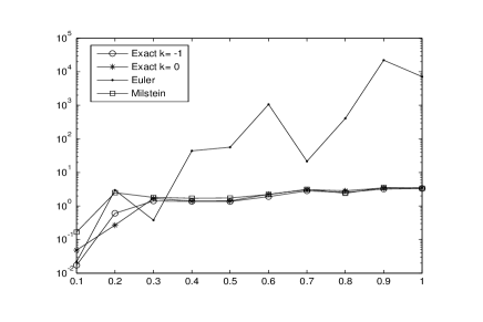

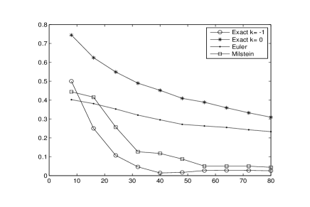
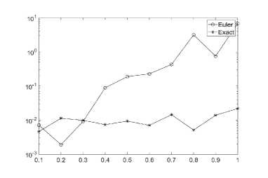
In Figure 2 we report the weak and strong errors with respect to the maximum time of integration , which varies from to , and stepsize . In this situation also the errors of the Mistein method remain bounded. In other words belongs to the stability region of the Milstein method but not to the stability region of the Euler method.


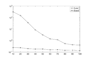
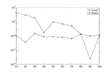
In Figure 3 we plot the weak and strong errors with fixed final time and steps number , where the stepsize . Here we note that the weak and strong errors for the exact methods do not change with the stepsize. This means that with a stepsize of only the exact methods have weak and strong systematic errors less than the statistical errors. Instead for the Milstein scheme the errors grow and only with a stepsize equal to the systematic errors are comparable with the statistical ones. Equivalently we can say that the stability region is . In the Euler case the systematic error is not comparable with the statistical one.
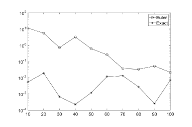
In Figure 4 we report the total variation distance between the empirical probabilities of and of obtained simulating paths. We note that there is a big difference between the exact method for and for . The discrepancy is due to the fact that the exact method with tends to overestimate the points with probability less then more than the Euler scheme does.
Now we simulate the two dimensional linear SDE analized in Section 4 by
choosing and . Our choice of the parameters guarantees the existence of an equilibrium probability density.
We compare approximated solutions obtained with the Euler method and with our exact method using . To this end we calculated both the strong and weak componentwise error
| (42) | ||||
| (43) |
where is the th component of the solution. This time our true solution is calculated using the Euler method with timestep . As in the previous example the error are estimated using a Montecarlo simulation, this time with paths, both for the approximated and the true solution. Again we expect and to include both systematic and statistical errors.
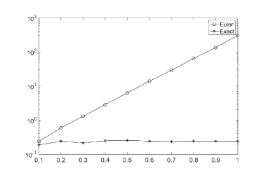
In Figure 5 and Figure 6 we compare the strong and weak error of both components of the simulated solutions with respect to the maximum time of integration varying from to . As can be seen the error from our new method is bounded at all times while the Euler method errors show an exponential growth with respect to the maximum time.
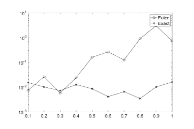
In Figure 7 and Figure 8 we compare the errors of both approximations for solutions with and timestep size varying between to . As in the previous one-dimensional case we can see how the new exact method gives a good approximation of the true solution even with large timesteps, while the Euler method fails to achieve the same magnitude of error even using a significative smaller timesteps.
7 Appendix
In the proof of Theorem 5.1, by using Lemma 5.3 and the independence of Brownian increments, we can estimate the errors in a very explicitely way. In particular without exploiting Lemma 5.4. We show main steps and final expressions.
From (33) we obtain that
with
Since , then with and, finally,
where is given by (35), according with (34).
From (37) we obtain
where
Since , we have that with and
according with (38).
The second term on the right-hand side of (36) becomes
where we have used independence and we have set
We can obtain
and, since , that , where Being:
by putting , one can easily verify that
(because ) and, therefore, , where Finally
that is
with
References
- [1] Cristina Anton, Jian Deng, and Yau Shu Wong. Weak symplectic schemes for stochastic Hamiltonian equations. Electron. Trans. Numer. Anal., 43:1–20, 2014/15.
- [2] Nawaf Bou-Rabee and Houman Owhadi. Stochastic variational integrators. IMA J. Numer. Anal., 29(2):421–443, 2009.
- [3] Nawaf Bou-Rabee and Houman Owhadi. Long-run accuracy of variational integrators in the stochastic context. SIAM J. Numer. Anal., 48(1):278–297, 2010.
- [4] Rutwig Campoamor-Stursberg, Miguel A. Rodríguez, and Pavel Winternitz. Symmetry preserving discretization of ordinary differential equations. Large symmetry groups and higher order equations. J. Phys. A, 49(3):035201, 21, 2016.
- [5] Chuchu Chen, David Cohen, and Jialin Hong. Conservative methods for stochastic differential equations with a conserved quantity. Int. J. Numer. Anal. Model., 13(3):435–456, 2016.
- [6] Francesco C. De Vecchi. Lie symmetry analysis and geometrical methods for finite and infinite dimensional stochastic differential equations. PhD thesis, 2017.
- [7] Francesco C. De Vecchi, P. Morando, and S. Ugolini. A note on symmetries of diffusions within a martingale problem approach. Stochastics and Dynamics.
- [8] Francesco C. De Vecchi, Paola Morando, and Stefania Ugolini. Reduction and reconstruction of stochastic differential equations via symmetries. J. Math. Phys., 57(12):123508, 22, 2016.
- [9] Francesco C. De Vecchi, Paola Morando, and Stefania Ugolini. Symmetries of stochastic differential equations: a geometric approach. J. Math. Phys, 57(6):063504, 17, 2016.
- [10] Vladimir Dorodnitsyn. Applications of Lie groups to difference equations, volume 8 of Differential and Integral Equations and Their Applications. CRC Press, Boca Raton, FL, 2011.
- [11] K. Ebrahimi-Fard, A. Lundervold, S. J. A. Malham, H. Munthe-Kaas, and A. Wiese. Algebraic structure of stochastic expansions and efficient simulation. Proceedings of the Royal Society A: Mathematical, Physical and Engineering Sciences, 468(2144):2361–2382, apr 2012.
- [12] Nicola Bruti-Liberati Eckhard Platen. Numerical Solution of Stochastic Differential Equations with Jumps in Finance. Springer Berlin Heidelberg, 2010.
- [13] Avner Friedman. Stochastic differential equations and applications. Vol. 1. Academic Press [Harcourt Brace Jovanovich, Publishers], New York-London, 1975. Probability and Mathematical Statistics, Vol. 28.
- [14] Peter Friz and Sebastian Riedel. Convergence rates for the full Gaussian rough paths. Ann. Inst. Henri Poincaré Probab. Stat., 50(1):154–194, 2014.
- [15] Peter K. Friz and Martin Hairer. A course on rough paths. Universitext. Springer, Cham, 2014. With an introduction to regularity structures.
- [16] Giuseppe Gaeta and Niurka Rodríguez Quintero. Lie-point symmetries and stochastic differential equations. J. Phys. A, 32(48):8485–8505, 1999.
- [17] Ernst Hairer, Christian Lubich, and Gerhard Wanner. Geometric numerical integration, volume 31 of Springer Series in Computational Mathematics. Springer-Verlag, Berlin, second edition, 2006. Structure-preserving algorithms for ordinary differential equations.
- [18] Diego Bricio Hernández and Renato Spigler. -stability of Runge-Kutta methods for systems with additive noise. BIT, 32(4):620–633, 1992.
- [19] Desmond J. Higham. Mean-square and asymptotic stability of the stochastic theta method. SIAM J. Numer. Anal., 38(3):753–769 (electronic), 2000.
- [20] Desmond J. Higham and Peter E. Kloeden. Numerical methods for nonlinear stochastic differential equations with jumps. Numer. Math., 101(1):101–119, 2005.
- [21] Desmond J. Higham, Xuerong Mao, and Chenggui Yuan. Almost sure and moment exponential stability in the numerical simulation of stochastic differential equations. SIAM J. Numer. Anal., 45(2):592–609 (electronic), 2007.
- [22] Darryl D. Holm and Tomasz M. Tyranowski. Variational principles for stochastic soliton dynamics. Proc. A., 472(2187):20150827, 24, 2016.
- [23] Jialin Hong, Shuxing Zhai, and Jingjing Zhang. Discrete gradient approach to stochastic differential equations with a conserved quantity. SIAM J. Numer. Anal., 49(5):2017–2038, 2011.
- [24] Arieh Iserles. A first course in the numerical analysis of differential equations. Cambridge Texts in Applied Mathematics. Cambridge University Press, Cambridge, second edition, 2009.
- [25] Peter E. Kloeden and Eckhard Platen. Numerical solution of stochastic differential equations, volume 23 of Applications of Mathematics (New York). Springer-Verlag, Berlin, 1992.
- [26] Roman Kozlov. Symmetries of systems of stochastic differential equations with diffusion matrices of full rank. J. Phys. A, 43(24):245201, 16, 2010.
- [27] Joan-Andreu Lázaro-Camí and Juan-Pablo Ortega. Reduction, reconstruction, and skew-product decomposition of symmetric stochastic differential equations. Stoch. Dyn., 9(1):1–46, 2009.
- [28] Benedict Leimkuhler and Sebastian Reich. Simulating Hamiltonian dynamics, volume 14 of Cambridge Monographs on Applied and Computational Mathematics. Cambridge University Press, Cambridge, 2004.
- [29] Paul Lescot and Jean-Claude Zambrini. Probabilistic deformation of contact geometry, diffusion processes and their quadratures. In Seminar on Stochastic Analysis, Random Fields and Applications V, volume 59 of Progr. Probab., pages 203–226. Birkhäuser, Basel, 2008.
- [30] Decio Levi, Peter Olver, Zora Thomova, and Pavel Winternitz, editors. Symmetries and integrability of difference equations, volume 381 of London Mathematical Society Lecture Note Series. Cambridge University Press, Cambridge, 2011. Lectures from the Summer School (Séminaire de Máthematiques Supérieures) held at the Université de Montréal, Montréal, QC, June 8–21, 2008.
- [31] Decio Levi and Pavel Winternitz. Continuous symmetries of difference equations. J. Phys. A, 39(2):R1–R63, 2006.
- [32] Simon J. A. Malham and Anke Wiese. Stochastic Lie group integrators. SIAM J. Sci. Comput., 30(2):597–617, 2008.
- [33] Sergey V. Meleshko, Yurii N. Grigoriev, Nail K. Ibragimov, and Vladimir F. Kovalev. Symmetries of integro-differential equations: with applications in mechanics and plasma physics, volume 806. Springer Science & Business Media, 2010.
- [34] Grigori N. Milstein, E. Platen, and H. Schurz. Balanced implicit methods for stiff stochastic systems. SIAM J. Numer. Anal., 35(3):1010–1019 (electronic), 1998.
- [35] Grigori N. Milstein, Yu. M. Repin, and M. V. Tretyakov. Numerical methods for stochastic systems preserving symplectic structure. SIAM J. Numer. Anal., 40(4):1583–1604 (electronic), 2002.
- [36] Peter J. Olver. Applications of Lie groups to differential equations, volume 107 of Graduate Texts in Mathematics. Springer-Verlag, New York, second edition, 1993.
- [37] Étienne. Pardoux and Philip E. Protter. A two-sided stochastic integral and its calculus. Probab. Theory Related Fields, 76(1):15–49, 1987.
- [38] G. Reinout W. Quispel and Robert I. McLachlan. Special issue on geometric numerical integration of differential equations’. Journal of Physics A: Mathematical and General, 38(10):null, 2005.
- [39] Yoshihiro Saito and Taketomo Mitsui. Stability analysis of numerical schemes for stochastic differential equations. SIAM J. Numer. Anal., 33(6):2254–2267, 1996.
- [40] Molei Tao, Houman Owhadi, and Jerrold E. Marsden. Nonintrusive and structure preserving multiscale integration of stiff ODEs, SDEs, and Hamiltonian systems with hidden slow dynamics via flow averaging. Multiscale Model. Simul., 8(4):1269–1324, 2010.
- [41] Angel Tocino. Mean-square stability of second-order Runge-Kutta methods for stochastic differential equations. J. Comput. Appl. Math., 175(2):355–367, 2005.
- [42] Lijin Wang, Jialin Hong, Rudolf Scherer, and Fengshan Bai. Dynamics and variational integrators of stochastic Hamiltonian systems. Int. J. Numer. Anal. Model., 6(4):586–602, 2009.
- [43] Chenggui Yuan and Xuerong Mao. Stability in distribution of numerical solutions for stochastic differential equations. Stochastic Anal. Appl., 22(5):1133–1150, 2004.