Spatial uniformity in power-grid system

Abstract

Robust synchronization is indispensable for stable operation of a power grid. Recently, it has been reported that a large number of decentralized generators, rather than a small number of large power plants, provide enhanced synchronization together with greater robustness against structural failures. In this paper, we systematically control the spatial uniformity of the geographical distribution of generators, and conclude that the more uniformly generators are distributed, the more enhanced synchronization occurs. In the presence of temporal failures of power sources, we observe that spatial uniformity helps the power grid to recover stationarity in a shorter time. We also discuss practical implications of our results in designing the structure of a power-grid network.

I Introduction

The emergence of synchronization has been an important issue in the statistical physics community. It has been observed in a variety of phenomena like the circadian rhythm Kolmos and Davis (2007), epilepsy in the brain Fisher et al. (2005), and the London Millennium Bridge Strogatz et al. (2005). Examples of synchronization phenomena exist also in social behaviors Silverberg et al. (2013); Hoang et al. (2015) and in the power grid Filatrella et al. (2008). It is to be noted that the emergence of synchronization can be desirable or not, depending on what is required for a given system to function properly. For example, an epileptic seizure in a human brain and a large vibration of the London Millennium Bridge are caused by undesired synchronization, and recent research has reported how to inhibit such unwanted synchronization behavior Louzada et al. (2012). In contrast, for the power grid, which is the main focus of the present paper, robust synchronization is an essential ingredient for the system to work in a stable manner. If a power plant in the grid is not running at a proper reference frequency, or the phase angle of the voltage produced by the plant does not match that of the grid, the plant cannot properly convey electric power to the grid, and it is possible to result in a short circuit and damage to the generator Mazloomzadeh et al. (2012); Croft and Summers (1987). A malfunctioning generator can yield cascading failures in the grid in the worst case, leading to a large-scale blackout.

Synchronization in the power-grid system has been studied from various points of view. The swing equation, which is similar to the Kuramoto model in statistical physics, has been suggested to describe the dynamics of the power-grid system Filatrella et al. (2008); Nishikawa and Motter (2015). Stability of the synchronized state is also an important issue and has been studied through the use of several methods such as the basin stability Menck et al. (2013); Kim et al. (2016) and the Lyapunov exponent Li and Wong . A power grid is of course a typical example of complex networks. From this perspective, the impact of the network structure on the synchronous state Rohden et al. (2014) and the optimal network topology for enhanced synchronization Pinto and Saa (2016) have been investigated.

An interesting finding in existing studies is that decentralized generators provide enhanced synchronization together with robustness against structural failures Rohden et al. (2012). This is a particularly important result in view of the growing recent interest in renewable energy sources. If a large number of small generators based on renewable sources are connected in the power grid in the form of a complex network, understating of the effect of decentralized power generators can be very important.

In this work, we focus on how to distribute decentralized power generators in two-dimensional space to enhance the synchronization of the power grid. We control spatial uniformity of generators in two ways: First, we divide the whole two-dimensional area into available and unavailable regions for the positions of power plants and study how the change of the available area affects synchronization. Second, we impose various sizes of superlattice unit cells on top of the original two-dimensional square lattice. In each superlattice unit cell, power plants are put near the center of the unit cell. In the limiting case where one superlattice unit cell covers the whole system, all plants are put only in the central part of the whole region. As the size of the superlattice becomes smaller, power plants tend to be spread more uniformly across the whole system.

The present paper is organized as follows: In Sec. II, we introduce the Kuramoto model with inertia to describe the dynamics of the power grid Filatrella et al. (2008). We also check how the synchronization behavior depends on the system size and the number of generators. In Sec. III, we describe how we control the spatial uniformity of generators in two dimensions in two different ways, and explain our results. Section IV is devoted to a discussion and summary.

II Equation of Motion for The Power Grid

We sketch the derivation of the equation of motion for a power grid in Ref. Filatrella et al. (2008). The power grid is composed of two types of nodes, generators and consumers. A consumer node in this work may represent a large group of consumers in reality, like a city. Energy from a natural source is first converted to mechanical energy, and an electric generator then converts it to electric energy. In a hydroelectric power plant, for instance, the gravitational potential energy of water in a dam is converted to the rotational kinetic energy of a turbine, which generates an alternating current (ac) electric power via Faraday’s law of electromagnetic induction. In a thermal power plant based on a fossil energy source, the chemical energy in the fuel is used to boil the water, and the pressure from the steam provides the mechanical rotational energy injected into an electric generator.

In this work we denote the mechanical energy injected into a turbine of the generator at node $i$ as $P_{i}$. The dynamic variable for a generator node in the power grid is the turbine’s rotational phase angle, which is directly related to the phase of the ac voltage generated from the generator. We assume that the former equals the latter and write it as $\theta_{i}$ for the generator node $i$. In the research community of the power grid, the consumer node $j$ is also assigned the phase variable $\theta_{j}$ in the same way as for the generator node. One can assume that each consumer has an electric motor to convert the supplied electric power into mechanical power, and $\theta_{j}$ is either the rotational phase angle of the motor or the phase of the voltage for the consumed power. For both the generator and the consumer nodes, the instantaneous phase at the $i$th node is written as $\theta_{i}(t)=\Omega t+\phi_{i}(t)$, where $\Omega=2\pi f$ with a grid reference frequency $f=60$ or 50 Hz, and $\phi_{i}(t)$ measures the deviation from the rotating reference frame.

The injected mechanical energy is then transformed to the rotational kinetic energy of the turbine (the motor) of the generator (the consumer) node and the electric energy to be transmitted to other nodes in the power grid. Of course, some part of the injected energy is lost in the form of dissipation due to friction. Accordingly, one can write the energy (or the power) conservation condition in the form

$$P_{i}=P_{\textrm{kin},i}+P_{\textrm{diss},i}+\sum_{j}P_{\textrm{trans},ij},$$ (1)

where $P_{\textrm{kin}}$ and $P_{\textrm{diss}}$ are powers corresponding to the rotational kinetic energy and the dissipated energy, respectively, and the last term is the power transmitted from $i$ to other connected nodes in the power grid. The power, the energy per unit time, for the rotational kinetic energy is given by $P_{\textrm{kin},i}=\frac{d}{dt}\left(\frac{1}{2}I\dot{\theta}_{i}^{2}\right)$ with the moment of inertia $I$ of the turbine or the motor. The power for the dissipated energy is written as $P_{\textrm{diss},i}=\kappa\dot{\theta}_{i}^{2}$ with the dissipation coefficient $\kappa$. The power transmitted from $i$ to $j$ through a transmission line is written as $P_{\textrm{trans},ij}=P_{\textrm{max}}A_{ij}\sin(\theta_{i}-\theta_{j})$, where $P_{\textrm{max}}$ is the maximum allowed value of the transmitted power, and $A_{ij}$ is the element of the symmetric adjacency matrix, i.e., $A_{ij}=A_{ji}=1$ if $i$ and $j$ are connected, and $A_{ij}=A_{ji}=0$ otherwise. (See Appendix A for the calculation of the transmitted power.) We remark that although the present work focuses on a two-dimensional square grid with only geographically local couplings, it is straightforward to apply our framework to a general adjacency matrix which may describe very long transmission cables in the power grid.

Under the realistic assumption that the power grid works almost at the reference angular frequency $\Omega$, i.e., $\dot{\theta}_{i}=\Omega+\dot{\phi}_{i}\approx\Omega$ and thus $|\dot{\phi_{i}}|\ll\Omega$, we obtain $P_{\textrm{kin},i}\approx I\ddot{\phi_{i}}\Omega$ and $P_{\textrm{diss},i}\approx\kappa\Omega^{2}+2\kappa\Omega\dot{\phi_{i}}$. Using $\theta_{j}-\theta_{i}=\phi_{j}-\phi_{i}$, Eq. (1) is then written as

$$\ddot{\phi_{i}}=\bar{P}_{i}-\alpha\dot{\phi_{i}}+K\sum_{j=1}^{N}A_{ij}\sin(\phi_{j}-\phi_{i}),$$ (2)

where $N$ is the size of the power grid, $\bar{P}_{i}\equiv(P_{i}-\kappa\Omega^{2})/I\Omega$, $\alpha\equiv 2\kappa/I$, and $K\equiv P_{\textrm{max}}/I\Omega$. It is to be noted that a power generating node can have a negative value of the net power ($\bar{P}_{i}<0)$ if the injected mechanical power is less than the rotational kinetic power. Henceforth we regard a node as a generator (a consumer) if $\bar{P}_{i}>0$ ($\bar{P}_{i}<0$).

The power conservation equation, (2), for the stationary state $\dot{\phi}_{i}=\ddot{\phi}_{i}=0$ is written as $0=\bar{P}_{i}+K\sum_{j}A_{ij}\sin(\phi_{j}-\phi_{i})$, and thus we get the power balance condition $\sum_{i}\bar{P}_{i}=0$ from the symmetry $A_{ij}=A_{ji}$ of the adjacency matrix. It is important to note that if the conservation of the total power, i.e., $\sum_{i}\bar{P}_{i}=0$, is violated, the system cannot have a stationary state. In the present work, we assume that all generator nodes have equal power generating capacity (except in Appendix B where we discuss the case for a few large power plants at the boundary) and all consumer nodes consume an equal amount of power. In other words, we use $\bar{P}_{i}=cP$ for a generator node, and $\bar{P}_{i}=-P$ for a consumer node, respectively, with $P>0$. The positive constant $c$ is simply determined from $\sum_{i}\bar{P}_{i}=0$. Note that as the number of generators $N_{\rm gen}$ is decreased the power provided by each power plant should increase, i.e., $c$ is a decreasing function of $N_{\rm gen}$ since $c=N/N_{\rm gen}-1$. Since the population density in the real world is well-known to be nonuniform, the above assumption that all consumer nodes have the same value of power consumption cannot be valid in reality. Nevertheless, we emphasize that our framework can easily be modified once the power consumption of each consumer node is determined from the real data. Similarly to Ref. Witthaut and Timme (2012), we set $\alpha\equiv 1$ and $P\equiv 1$ for convenience.

We use the initial condition $\phi_{i}(t=0)=0$ and numerically integrate the equation of motion in Eq. (2) by using the second-order Runge-Kutta algorithm Press et al. (1992) with the discrete time step $\Delta t=0.001$ till $t=T$ is approached. For given constraints such as the system size $N$, the number of generator nodes $N_{\rm gen}$, and the available region for them, we randomly choose the generator nodes among available nodes on a two-dimensional square lattice (remaining nodes become consumer nodes). Each sample with a random realization of generator nodes is evolved in time, and it is observed that some samples eventually approach stationary states and others do not. We check how long we need to wait to judge whether or not the system eventually arrives at the stationary state and find that $T=150$ and $T=200$ do not make any difference. In other words, if the system arrives at a stationary state, it does so well before $T=150$. If the system does not settle down to a stationary state before $T=150$, it remains in a nonstationary state even after $T=200$. As a key quantity to measure the global synchrony at a given coupling constant $K$, we use the conventional order parameter $r(t)$ for the Kuramoto model,

$$r(t)\equiv\frac{1}{N}\left|\sum_{j}e^{i\phi_{j}(t)}\right|.$$ (3)

If the system does not arrive at the stationary state till $t=T(=200)$, we suppose that the system will be nonstationary to eternity and assign the value $m=0$ for our order parameter $m$. If the system approaches the stationary state much earlier than $T=200$, we assign $m=r(T=200)$. We take the ensemble average over 200 different realizations of generator nodes to get $\langle m\rangle$. The logic behind the above definition of the order parameter is that $m$ must have a nonzero value for the power grid to function properly. If the power grid keeps fluctuating without settling down to the stationary state, our definition of $m$ indicates failure of the power grid. Otherwise, if the power grid approaches a stationary state but the level of synchrony is not good enough, our definition of $m$ also indicates failure of the power grid.

Figure 1: (Color online) Ensemble average of the order parameter $\langle m\rangle$ versus coupling strength $K$ when power generators are randomly placed on a two-dimensional square lattice of the size $N=L\times L$. (a) We fix the generator density $N_{\rm gen}/N\approx 0.2$ and vary the system size. ($N_{\rm gen}=9,25,$ and $49$ for $L=7,11,$ and $15$, respectively.) (b) We fix the system size $L=15$ and vary the number of generators $N_{\rm gen}=25,49,$ and $81$. From (a) and (b), we conclude that the level of synchrony is a decreasing function of the system size $L$ and an increasing function of the number of generators $N_{\rm gen}$.

In Fig. 1(a), we show the ensemble average (over 200 samples) of the order parameter $\langle m\rangle$ versus the coupling strength $K$ for various sizes $N=(L\times L)$ of two-dimensional square lattices at almost the same value of the generator density $N_{\textrm{gen}}/N$: $N_{\rm gen}=9,25,$ and $49$ are used for $L=7,11,$ and $15$ (and thus the generator density $N_{\textrm{gen}}/N\approx 0.2$). Positions of generators are randomly picked in the whole system. In Fig. 1(a), it is clearly shown that as the system size is increased, $\langle m\rangle$ is decreased at any value of $K$, which is in accord with the known result that the locally coupled oscillators in two dimensions are not synchronized at any finite value of $K$ in the thermodynamic limit Hong et al. (2004). We thus expect that if $L$ is increased further $\langle m\rangle\rightarrow 0$ for any $K$. However, a power grid in the real world is always of a finite size, and we are interested only in how to distribute generators for a given system size.

In Fig. 1(b), we plot $\langle m\rangle$ versus $K$ for $N_{\textrm{gen}}=25,49,$ and $81$ at the fixed system size of $L=15$. One can understand the observed behavior that the same level of $\langle m\rangle$ is achieved at a lower value of $K$ when the number of generators is larger as follows: The coupling constant $K$ in our model plays the role of the capacity of the power transmission cable. Consequently, as the number of generators becomes larger, the power that each generator should supply becomes less, and thus we can achieve a sufficient level of synchrony with a smaller value of $K$. From the above investigations in Fig. 1(a) and  1(b), the roles played by the number of generators and the size of the system can be summarized in a simple manner: The level of synchrony is reduced for a larger system size and for fewer generators. Accordingly, henceforth, we fix the system size and the number of generators and focus on the effect of the pattern of the spatial distribution of generators. Also note that our result in Fig. 1(b) is consistent with the finding that decentralized generators exhibit better synchrony Rohden et al. (2012).

Figure 2: (Color online) Method 1: Control of spatial uniformity by changing the available region for generators. The two-dimensional square lattice of linear size $L$ is divided into two regions (gray and yellow). The yellow region between the outer square of size $L_{2}$ and the inner square of size $L_{1}$ is allowed for generator locations. Among all $S=L_{2}^{2}-L_{1}^{2}$ points in the available yellow region, $N_{\rm gen}$ points are randomly selected as positions of generators. (b) An example realization of generator positions (brown circles). Small black squares are the locations of consumers.

III Spatial Uniformity and Synchronization

In this section, we propose two methods to control the spatial uniformity of generators in a power grid in two dimensions: First, we define the region in which generators can be located as the outside of the square of the linear size $L_{1}$ and the inside of the square of the linear size $L_{2}$. The centers of both squares coincide with the central position of the whole two-dimensional power grid. As $L_{1}$ and $L_{2}(>L_{1})$ are changed (and so is the available area $S\equiv L_{2}^{2}-L_{1}^{2}$) the degree of spatial uniformity of the generator distribution is systematically altered. Second, we place a superlattice structure of linear size $l$ on top of the underlying square lattice, and put a given number of generators in the central region in each superlattice unit cell. Generators are spread more uniformly for small $l$, and in the limiting case where $l$ equals the linear size $L$ of the whole system the spatial uniformity is the lowest. We describe our results for the first method (using $L_{1}$ and $L_{2}$) of changing the available region in Sec. III.1 and for the second method (using various sizes $l$ of superlattices) in Sec. III.2.

III.1 Method 1: Change of available region

Figure 2(a) illustrates how we control the spatial distribution of generators by changing the region available for generator locations. Note that the power-grid network in the present work has the structure of a conventional square lattice of size $N=L\times L$ in two dimensions, with the open boundary condition. We believe that use of the open boundary condition rather than the periodic boundary condition makes much more sense since most power plants in reality often provide electric power only within a country. In our model system, each node which is not on the boundary in the power grid has four nearest neighbors with equal degree $k=4$. We use two squares of sizes $L_{1}$ and $L_{2}$, and only the region between the inner ($L_{1}$) and the outer ($L_{2}$) squares [yellow region in Fig. 2(a)] is allowed for the locations of generators. The allowed region has width $w\equiv(L_{2}-L_{1})/2$ and area $S\equiv L_{2}^{2}-L_{1}^{2}$. (Note that $0\leq L_{1}<L_{2}\leq L$.) In the allowed region of the area $S$, we put $N_{\rm gen}$ generators at randomly chosen positions ($N_{\rm gen}\leq S$). As an example, one random realization of generator locations is depicted in Fig. 2(b) for $L=11$, $N_{\textrm{gen}}=25$, $L_{1}=3$, and $L_{2}=7$ (and thus $w=2$ and $S=40$).

Figure 3: (Color online) We change the spatial uniformity as depicted in Fig. 2 for a given number of generators $N_{\rm gen}=49$ for a power grid of size $L=15$. The synchronization order parameter $\langle m\rangle$ versus the coupling constant $K$ (a) for various values of $L_{2}$ at fixed $L_{1}=0$ and (b) for various values of $L_{1}$ at fixed $L_{2}=L=15$. (c, d) Normalized histograms $P(f)$ for the power transmitted through each link at $K=7$, corresponding to (a) and (b), respectively, are displayed as a color map. The lines for $\bar{f}\equiv\sum_{f}fP(f)$ and for $f^{*}\equiv\arg\max P(f)$ are also shown. It is clearly shown that as generators are more uniformly spread in space [as $L_{2}$ is increased in (c) and as $L_{1}$ is decreased in (d)], $f$ tends to have small values. (e, f) Scatter-plots of $m$ versus $n_{c}$ [see Eq. (5)] at $K=7$, corresponding to (c) and (d), respectively.

In order to check the effect of spatial uniformity for a given number of generators placed in the given size of the system, we fix $L=15$ and $N_{\rm gen}=49$, and change $L_{1}$ and $L_{2}$ systematically. In Fig. 3(a), we fix the size of the inner square to $L_{1}=0$, and vary $L_{2}$ from 7 to 15. For $L_{2}=7$, all generators are densely packed in the central part of the power grid since $S=N_{\rm gen}=49$, while for $L_{2}=L=15$ generators are randomly distributed across the whole system. It is observed that the degree of synchrony is enhanced with $L_{2}$ for $L_{2}=7,9,$ and $11$. Interestingly, results for $L_{2}=13$ and $15$ do not exhibit much difference. In Fig. 3(b), we fix the size of the outer square to $L_{2}=L=15$, and vary $L_{1}$ instead. Similarly to Fig. 3(a), it is shown that the synchronization is enhanced as the area available for generators becomes larger.

We next look into the power transmitted through each link from the expectation that a link can be overloaded if the link carries too much power and thus it is desirable that the power at each link is evenly spread over the whole grid. The power transmitted from node $i$ to node $j$ is given by

$$F_{ij}=-F_{ji}=K\sin(\theta_{i}-\theta_{j}),$$ (4)

with $K$ being the maximum allowed value for transmission. We measure $|F_{ij}|$ for each pair of links and construct the normalized histogram $P(f\equiv|F|/K)$ of the power transmission with bin size $\Delta f=0.02$. We measure $P(f)$ at $K=7$ for the cases shown in Figs. 3(a) and 3(b), and display our results in Figs. 3(c) and 3(d), respectively. The value $K=7$ is chosen since all curves at this value of $K$ exhibit sufficiently large values of $\langle m\rangle$ as shown in Figs. 3(a) and 3(b). In Figs. 3(c) and 3(d), the color of each small circle indicates the value of $P(f)$ (see the color bar). We also measure the average value $\bar{f}\equiv\sum_{f}fP(f)$ and the peak position $f^{*}\equiv\arg\max P(f)$ and display them in Figs. 3(c) and 3(d). It is shown that as the generators are more evenly distributed in the power grid, i.e., as $L_{2}$ is increased [Figs. 3(a) and 3(c)], and as $L_{1}$ is decreased [Figs. 3(b) and 3(d)], the synchronization is enhanced [Figs. 3(a) and 3(b)] and the transmitted power of links is more focused on small values [see also the curves for $\bar{f}$ and $f^{*}$ in Figs. 3(c) and 3(d)].

Figure 4: (Color online) Scatter plot for $m$ versus $n_{c}$ at $K=7$ for $L=15$ and $N_{\rm gen}=49$. To elaborate the effect of $n_{c}$ for a fixed value of $S=L_{2}^{2}-L_{1}^{2}$, we use the parameter values $(L_{1},L_{2})=(5,9),(13,15)$ for $S=56$, $(3,9),(7,11)$ for $S=72$, and $(1,11),(7,13)$ for $S=120$. Positive correlations between $m$ and $n_{c}$ are seen. The number of samples is 200, and the ensemble averages of $m$ and $n_{c}$ are represented as black squares, together with the error bars.

If power plants are packed into a certain narrow region of the whole system, we believe that the global synchrony may be reduced. As suggested by the expectation, we measure the number of consumer nodes for which a generator node provides the power directly. The average number of direct consumers per generator is given by

$$n_{c}\equiv\frac{1}{N_{\rm gen}}\sum_{i,j}^{\prime}A_{ij},$$ (5)

where the primed summation is for the pair $(i,j)$, with $i$ ($j$) being a generator (a consumer). In our two-dimensional square lattice structure for the power grid, the maximum value of $n_{c}$ is $4$, the number of nearest neighbors for the square lattice. In Figs. 3(e) and 3(f), we display the scatter plots for $m$ versus $n_{c}$ at $K=7$, for $L_{1}=0$ and $L_{2}=7,9,11,13,$ and $15$ and for $L_{2}=15$ and $L_{1}=1,5,9,13$, corresponding to Figs. 3(a) and 3(c), and Figs. 3(b) and 3(d), respectively. In Fig. 3(e), $m$ is increasing with $n_{c}$, implying that the synchronization is more enhanced as the number of direct connections between generators and consumers is increased.

We have shown above that the spatial uniformity for the generator distribution is closely related to the synchrony of the power grid. In general, as the region available for generator locations becomes larger, i.e., as the area $S$ is increased, the synchronization order parameter $m$ becomes larger. We have also checked the importance of the average number $n_{c}$ of direct consumers per generator and have shown that as $n_{c}$ is increased, so is $m$. The next question one can ask is, What happens if $n_{c}$ can be varied for a given area $S$? To answer the question, we use pairs of sizes $(L_{1},L_{2})=(5,9),(13,15)$ for $S=56$, $(L_{1},L_{2})=(3,9),(7,11)$ for $S=72$, and $(L_{1},L_{2})=(1,11),(7,13)$ for $S=120$, for a system of size $L=15$ with the number of generators $N_{\rm gen}=49$ as for Fig. 3 at coupling strength $K=7$. Figure 4 displays how $m$ changes with $n_{c}$ for pairs of $(L_{1},L_{2})$ at fixed values of $S$. Again we observe that $m$ is an increasing function of $n_{c}$.

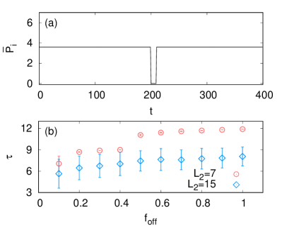
Figure 5: (Color online) (a) Temporal failure of a power generator is implemented as $\bar{P}_{i}=0$ for $200\leq t\leq 210$. (b) Recovery time $\tau$ versus fraction $f_{\rm off}$ of failed generators (see the text) for $L_{2}=7$ and 15. We have used $L_{1}=0$ and $K=8$. More uniformly distributed generators ($L_{2}=15$) exhibit shorter recovery times than less uniformly distributed generators ($L_{2}=7$).

We next investigate whether or not the spatial uniformity also yields a good performance against dynamic perturbation. It is noteworthy that uniformly spread plants of small powers can mimic renewable power sources, which can occasionally stop operating for various reasons. For example, a wind turbine may stop producing power if the wind becomes too weak in a certain period of time. To mimic such a temporal failure of power generation, we apply the following scenario: If the $i$-th power generator has a temporal problem, we change the power production $\bar{P}_{i}$ as depicted in Fig. 5(a). That is, $\bar{P}_{i}$ is set to $0$ only in the time interval $200\leq t\leq 210$, and before ($t<200$) and after ($t>210$) the failure, the power generation is set to $\bar{P}_{i}=cP$ as explained in Sec. II. We apply the failure scenario for a fraction $f_{\rm off}$ of randomly selected generators. Note that during the period of failures (i.e., for $200\leq t\leq 210$) the power balance condition $\sum_{i}{\bar{P}}_{i}=0$ is violated, and thus the power grid as a whole cannot stay in a stationary state. When the failed plants are back to work at $t=210$, the system is found to recover the original level of synchrony after a certain recovery time $\tau$. We fix $L_{1}=0$ and carry out simulations for $L_{2}=7$ and 15 at $K=8$ to investigate the effect of spatial uniformity on the recovery time $\tau$. Figure 5(b) displays the recovery time $\tau$ (averaged over 200 independent random realizations of plant locations and failed plants) versus the fraction $f_{\rm off}$ of turned-off power plants for $L_{2}=7$ and 15. It is clearly shown in Fig. 5(b) that the more uniformly power sources are distributed, the shorter the recovery time $\tau$ is. We thus conclude that spatial uniformity of the distribution of power plants helps the system to recover synchrony in shorter times.

To recap briefly, we have investigated how the uniformity of the spatial distribution of generators affects the degree of synchrony and the recovery after a temporal failure of power generation. As the generators are more uniformly distributed, $n_{c}$ becomes larger, leading to an enhancement of the synchronization. It is also observed that the recovery time becomes shorter for a more uniform distribution of generators. We thus conclude that the spatial uniformity of generator distribution is beneficial not only for better synchrony but also for better recovery behavior after a temporal perturbation of power generation.

Figure 6: (Color online) Method 2: Control of spatial uniformity by imposing superlattices. For a two-dimensional power-grid network of the size $16\times 16$, we placed superlattices of sizes $l\times l$ with $l=4,8,$ and $16$ and generators are packed near the center of each superlattice unit cell. The total number of generators is $N_{\rm gen}=64$. Positions of generators (consumers) are marked by brown circles (black squares) as in Fig. 2.

III.2 Method2: Change of superlattice unit cell

We next control the spatial uniformity of the generator distribution with the focus on the clustering effect. As depicted in Fig. 6, we place superlattice structures of different sizes $l$ of unit cells on top of the original two-dimensional $16\times 16$ square lattice. For a given superlattice of size $l\times l$, we put generators in the central part as in Fig. 6. The number of generators $N_{\rm gen}=64$ is fixed for the system size $N=16\times 16$ so that the generator density is 1/4, regardless of the value of $l$. Note that the smaller the superlattice is, the more uniformly the spatial distribution of generators becomes.

In Fig. 7(a), we plot the order parameter $m$ versus the coupling strength $K$ for $l=4,8$, and 16. It is clearly shown that as the size of the superlattice is increased, the global synchrony becomes worse. Since the positions of generators are given deterministically as shown in Fig. 6, the sample average is not needed. We then show in Fig. 7(b) how the average number $n_{c}$ of direct consumers per generator in Eq. (5) affects $m$. In accord with our previous observations for Figs. 3 and 4, it is clearly shown again that the spatial uniformity detected by $n_{c}$ is positively correlated with the enhancement of the synchrony of the power grid.

Figure 7: (Color online) The spatial uniformity is changed as in Fig. 6. for $N_{\rm gen}=64$ and $L=16$. (a) $m$ versus $K$ for superlattices of size $l=4,8$, and 16. As $l$ is increased, generators are more clustered, and the level of synchrony becomes worse. (b) $m$ versus $n_{c}$ at $K=7$.

IV Summary and Discussion

We have studied how the spatial uniformity in the distribution of power generators has an influence on the power-grid system. We have controlled the spatial uniformity, (i) by increasing the number of generators [Fig. 1(b)], and (ii) by increasing the available area for the generators [Figs. 3(a) and 3(b)], and have found that the number $n_{c}$ of power consumers directly connected to a generator is the key quantity: The synchronization order parameter $m$ has been found to increase as $n_{c}$ is increased. Even when the available area is fixed, $m$ has been shown to be positively correlated with $n_{c}$ (Fig. 4). We have also checked the clustering effect of generators for a given number of generators. It has again been confirmed that $m$ is an increasing function of $n_{c}$ also in this case (Fig. 7). We have also shown that when the global synchrony is enhanced the probability distribution of the transmitted power of a link tends to have peaks at small values of the power [Figs. 3(c) and 3(d)]. This is particularly interesting because the result indicates that the low values of power transmitted through transmission cables are accompanied by an enhanced synchrony of the power grid. It has been also confirmed that for more uniformly distributed generators the recovery time after a temporal perturbation is shorter, which again indicates that the spatial uniformity is beneficial (Fig. 5).

In order to better mimic a realistic distribution of power generators, we consider in Appendix B the presence of a few large power plants along the boundary of the system. Also in this case it is found that spatial uniformity of small generators tends to ensure better synchrony. We still believe that it could be difficult to apply our results directly to a real power-grid network. Nevertheless, we expect that our result will be useful to provide a guideline for designing a better power-grid structure.

Appendix A Power transmission through a link

Figure 8: A simple transmission line model. The circuit contains a resistor $R$ and an inductor $L$. The limit $R\rightarrow 0$ is taken when we compute the active power of the circuit.

In alternating current circuits at the angular frequency $\Omega$ depicted as a simple transmission line model in Fig. 8, a sender and a receiver are assigned complex voltages $V_{s}$ and $V_{r}$, respectively. The complex current is given by $I=(V_{s}-V_{r})/Z$, where the impedance $Z=R+iX_{L}$ with resistance $R$ and inductive reactance $X_{L}\equiv\Omega L$. The complex power $S$ in an ac circuit consists of the active power $P$ and the reactive power $Q$, i.e., $S=P+iQ=VI^{*}$ with the ac voltage $V$ and the complex conjugate $*$ of the electric current $I$. Accordingly, the complex powers $S_{s}$ for the sender and $S_{r}$ for the receiver are written as

$$S_{s} = P_{s}+iQ_{s}=V_{s}I^{*}=\frac{|V_{s}|^{2}-V_{s}V_{r}^{*}}{R-iX_{L}},$$

$$S_{r} = P_{r}+iQ_{r}=-V_{r}I^{*}=\frac{|V_{r}|^{2}-V_{r}V_{s}^{*}}{R-iX_{L}}.$$ (6)

We then use $V_{s}=|V_{s}|e^{i\gamma}$ and $V_{r}=|V_{r}|e^{i\delta}$ to get $|V_{s}|^{2}-V_{s}V_{r}^{*}=|V_{s}|^{2}-|V_{s}||V_{r}|(\cos\Delta\theta-i\sin\Delta\theta)$ and $|V_{r}|^{2}-V_{r}V_{s}^{*}=|V_{r}|^{2}-|V_{s}||V_{r}|(\cos\Delta\theta+i\sin\Delta\theta)$, with $\Delta\theta\equiv\gamma-\delta$, yielding

$$P_{s} = \frac{R(|V_{s}|^{2}-V_{s}V_{r}\cos\Delta\theta)-X_{L}V_{s}V_{r}\sin\Delta\theta}{R^{2}-X_{L}^{2}},$$

$$Q_{s} = -\frac{RV_{s}V_{r}\sin\Delta\theta+X_{L}(|V_{s}|^{2}-V_{s}V_{r}\cos\Delta\theta)}{R^{2}-X_{L}^{2}},$$

$$P_{r} = \frac{R(|V_{r}|^{2}-V_{s}V_{r}\cos\Delta\theta)+X_{L}V_{s}V_{r}\sin\Delta\theta}{R^{2}-X_{L}^{2}},$$

$$Q_{r} = -\frac{-RV_{s}V_{r}\sin\Delta\theta+X_{L}(|V_{r}|^{2}-V_{s}V_{r}\cos\Delta\theta)}{R^{2}-X_{L}^{2}}.$$ (7)

The active power $P$ in the limit of zero loss at the resistance ($R=0$) is then obtained as $P_{s}=-P_{r}=P_{\textrm{max}}\sin\Delta\theta$ with $P_{\textrm{max}}\equiv V_{s}V_{r}/X_{l}$ [see Eq. (2)].

Appendix B Spatial uniformity with a few large plants along the boundary

Figure 9: (Color online) (a) For the system discussed in Fig. 2, we place additional generators of large powers (denoted as larger circles) at fixed positions along the boundary to mimic a realistic distribution of larger plants along the coastline. (b) Scatter plots of $m$ versus $n_{c}$ for various vales of $L_{2}$ at fixed values of $L_{1}=0$ and $K=7$. Black squares represent averages over 200 sample runs.

In reality, we often have larger power plants along the coastline. To reflect this in our simple model, we introduce larger power plants at the boundary as in Fig. 9(a) and then control the spatial distribution of only smaller plants in the inland area (compare with Sec. III.1). We keep $N=N_{\rm gen}+N_{\rm con}=225$, $N_{\rm gen}=49$, and the demanding power of consumer $\bar{P}_{i}=-P$. Among $N_{\rm gen}$ generators, eight generators are regarded as large power plants with $\bar{P}_{i}=10P$, and they are located at fixed positions along the boundary [see Fig. 9(a)]. Other small generators produce the power $\bar{P}_{i}=c^{\prime}P$ and they are in the middle part of the system. A constant $c^{\prime}$ is determined from the power balance condition $\sum_{i}\bar{P}_{i}=0$. The generators with small powers are randomly distributed within the area formed by various values of $L_{2}$ at fixed $L_{1}=0$. Scatter-plots of $m$ versus $n_{c}$ at $K=7$ are shown in Fig. 9(b). The result demonstrates that the uniform distribution of small power plants helps to enhance the synchrony with increasing $n_{c}$, also in the more realistic case where large power plants are located at fixed positions along the boundary of the system.

References

- Kolmos and Davis (2007) E. Kolmos and S. J. Davis, Curr. Biol. 17, R808 (2007).
- Fisher et al. (2005) R. S. Fisher, W. v. E. Boas, W. Blume, C. Elger, P. Genton, P.Lee, and J. Engel, Epilepsia 46, 470 (2005).
- Strogatz et al. (2005) S. H. Strogatz, D. M. Abrams, A. McRobie, B. Eckhardt, and E. Ott, Nature (London) 438, 43 (2005).
- Silverberg et al. (2013) J. L. Silverberg, M. Bierbaum, J. P. Sethna, and I. Cohen, Phys. Rev. Lett. 110, 228701 (2013).
- Hoang et al. (2015) D.-T. Hoang, J. Jo, and H. Hong, Phys. Rev. E 91, 032135 (2015).
- Filatrella et al. (2008) G. Filatrella, A. H. Nielsen, and N. F. Pedersen, Eur. Phys. J. B 61, 485 (2008).
- Louzada et al. (2012) V. H. P. Louzada, N. A. M. Araújo, J. S. A. Jr., and H. J. Herrmann, Sci. Rep. 2, 658 (2012).
- Mazloomzadeh et al. (2012) A. Mazloomzadeh, V. Salehi, and O. Mohammed, in 2012 IEEE PES Innovative Smart Grid Technologies (ISGT) (IEEE, Washington, DC, 2012) p. 1.
- Croft and Summers (1987) T. Croft and W. Summers, American Electricans’ Handbook, Eleventh Edition (McGraw-Hill, New York, 1987).
- Nishikawa and Motter (2015) T. Nishikawa and A. E. Motter, New J. Phys. 17, 015012 (2015).
- Menck et al. (2013) P. J. Menck, J. Heitzig, N. Marwan, and J. Kruths, Nat. Phys. 9, 89 (2013).
- Kim et al. (2016) H. Kim, S. H. Lee, and P. Holme, Phys. Rev. E 93, 062318 (2016).
- (13) B. Li and K. Y. M. Wong, arXiv:1607.04509.
- Rohden et al. (2014) M. Rohden, A. Sorge, D. Witthaut, and M. Timme, Chaos 24, 013123 (2014).
- Pinto and Saa (2016) R. S. Pinto and A. Saa, Physica A 463, 77 (2016).
- Rohden et al. (2012) M. Rohden, A. Sorge, M. Timme, and D. Witthaut, Phys. Rev. Lett. 109, 064101 (2012).
- Witthaut and Timme (2012) D. Witthaut and M. Timme, New J. Phys. 14, 083036 (2012).
- Press et al. (1992) W. H. Press, S. A. Teukolsky, W. T. Vetterling, and B. P. Flannery, Numerical Recipes in C: The Art of Scientific Computing, 2nd ed. (Cambridge University Press, New York, USA, 1992).
- Hong et al. (2004) H. Hong, H. Park, and M. Y. Choi, Phys. Rev. E 70, 045204 (2004).