The Truncated Milstein Method for Stochastic Differential Equations

Abstract

Inspired by the truncated Euler-Maruyama method developed in Mao (J. Comput. Appl. Math. 2015), we propose the truncated Milstein method in this paper. The strong convergence rate is proved to be close to 1 for a class of highly non-linear stochastic differential equations. Numerical examples are given to illustrate the theoretical results.

Key words: Strong convergence rate, Non-linear stochastic differential equations, Truncated Milstein method, Non-global Lipschitz condition.

MAS Classification (2000): 65C20

1 Introduction

Stochastic differential equation (SDE), as a power tool to model uncertainties, has been broadly applied to many areas [1, 2, 3]. However, apart from linear SDEs, explicit solutions to most non-linear SDEs can hardly be found. Therefore, numerical approximations to SDEs become essential in the applications of SDE models.

When the drift and diffusion coefficients of SDEs satisfy the global Lipschitz condition, different kinds of numerical approximates have been broadly studied. We refer the readers to the monographs [4, 5, 6] for the detailed introductions and discussions.

Due to the simple structure and easy to programme, explicit methods, such as the Euler-Maruyama method, have been widely used [7]. But when the global Lipschitz condition is disturbed, the classical Euler-Maruyama method has been proved divergent [8, 9].

One of the natural candidates to tackle the divergence caused by the non-linearities in coefficients is implicit method. Many works have been devoted to implicit methods [10, 11, 12, 13, 14, 15, 16, 17, 18, 19, 20, 21]. Despite the good performance of the strong convergence, implicit methods have their own disadvantage that some non-linear systems need to be solved in each iteration, which may be computationally expensive and introduce some more errors.

Another way to tackle SDEs with non-global Lipschitz coefficients is to modify the drift and diffusion coefficients in the numerical methods. Following this approach, one can construct explicit methods that are able to converge to SDEs with coefficients allowed to grow super-linearly. The tamed Euler method [22, 23] is one of the most popular explicit methods that were developed particularly for the super-linear SDEs. In addition, we refer the readers to [24, 25, 26] for the simplified proofs of the strong convergence for the tamed Euler method, the tamed Milstein method and the semi-tamed method, respectively.

More recently, Mao in [27] proposed a new explicit method called the truncated Euler-Maruyama method. The new method focuses on those SDEs with both the drift and diffusion coefficients allowed to grow super-linearly. In [28], Mao further proved that the strong convergence rate of the method could be arbitrarily close to a half. Mao and his collaborators also studied the asymptotic behaviour of the method in [29].

Apart from the stand-alone research interests of the strong convergence of numerical methods, the property of the strong convergence could also be used to improve the convergence rate of estimating the expectation of some random variable by using the Multi-level Monte Carlo (MLMC) method [30]. Furthermore, Giles in [31] pointed out that a numerical method with the strong convergence rate of one could better cooperate with the MLMC method.

Therefore, in this paper we propose the truncated Milstein method, which is an explicit method and has the strong convergence rate of arbitrarily closing to one. In this work, both of the drift and diffusion coefficients of the SDEs under investigation could grow super-linearly.

This paper is organized as follows. Notations, assumptions and the truncated Milstein method will be introduced in Section 2. The proofs of the main results will be presented in Section 3. An example together with some ideas on further research will be presented in Section 4.

2 Mathematical Preliminaries

Throughout this paper, unless otherwise specified, let $(\Omega,{\cal F},\mathbb{P})$ be a complete probability space with a filtration $\left\{{\cal F}_{t}\right\}_{t\geq 0}$ satisfying the usual conditions (that is, it is right continuous and increasing while ${\cal F}_{0}$ contains all $\mathbb{P}$-null sets). Let $\mathbb{E}$ denote the expectation corresponding to $\mathbb{P}$. If $A$ is a vector or matrix, its transpose is denoted by $A^{T}$. Let $B(t)=(B^{1}(t),B^{2}(t),...,B^{m}(t))^{T}$ be an $m$-dimensional Brownian motion defined on the space. If $A$ is a matrix, let $|A|=\sqrt{\hbox{\rm trace}(A^{T}A)}$ be its trace norm. If $x\in\mathbb{R}^{d}$, then $|x|$ is the Euclidean norm. For two real numbers $a$ and $b$, set $a\vee b=\max(a,b)$ and $a\wedge b=\min(a,b)$. If $G$ is a set, its indicator function is denoted by $I_{G}$, namely $I_{G}(x)=1$ if $x\in G$ and $0$ otherwise.

Consider a $d$-dimensional SDE

$$dx(t)=f(x(t))dt+\sum_{j=1}^{m}g_{j}(x(t))dB^{j}(t)$$ (2.1)

on $t\geq 0$ with the initial value $x(0)=x_{0}\in\mathbb{R}^{d}$, where

$$f:\mathbb{R}^{d}\to\mathbb{R}^{d},\quad g_{j}:\mathbb{R}^{d}\to\mathbb{R}^{d},~{}j=1,2,...,m,$$

and $x(t)=(x^{1}(t),x^{2}(t),...,x^{d}(t))^{T}$.

In some of the proofs in this paper, we need the more specified notation that $f=(f_{1},f_{2},...,f_{d})^{T}$, $f_{i}:\mathbb{R}^{d}\rightarrow\mathbb{R}$ for $i=1,2,...,d$, and $g_{j}=(g_{1,j},g_{2,j},...,g_{d,j})^{T}$, $g_{i,j}:\mathbb{R}^{d}\rightarrow\mathbb{R}$ for $j=1,2,...,m$.

For $j_{1},j_{2}=1,...,m$, define

$$L^{j_{1}}g_{j_{2}}(x)=\sum_{l=1}^{d}g_{l,j_{1}}(x)\frac{\partial g_{j_{2}}(x)}{\partial x^{l}}.$$ (2.2)

For the truncated Milstein method, we need that both $f$ and $g$ have continuous second-order derivatives. In addition, the following assumptions are imposed.

Assumption 2.1

There exist constants $K_{2}>0$ and $r>0$ such that

$$|f(x)-f(y)|\vee|g_{j}(x)-g_{j}(y)|\vee\left|L^{j_{1}}g_{j_{2}}(x)-L^{j_{1}}g_{j_{2}}(y)\right|\leq K_{2}(1+|x|^{r}+|y|^{r})|x-y|$$

for all $x,y\in\mathbb{R}^{d}$ and $j,j_{1},j_{2}=1,2,...m$.

Assumption 2.2

For every $p\geq 1$, there exists a positive constant $K_{1}$, dependent on $p$, such that

$$\left\langle x-y,f(x)-f(y)\right\rangle+(2p-1)\sum_{j=1}^{m}\left|g_{j}(x)-g_{j}(y)\right|^{2}\leq K_{1}|x-y|^{2}$$

for all $x,y\in\mathbb{R}^{d}$.

Assumptions 2.1 and 2.2 guarantee that the SDE (2.1) has a unique global solution.

It is not hard to derive from Assumption 2.2 that for all $x\in\mathbb{R}^{d}$

$$\left\langle x,f(x)\right\rangle+(2p-1)\sum_{j=1}^{m}\left|g_{j}(x)\right|^{2}\leq\alpha_{1}(1+|x|^{2})$$ (2.3)

holds for all $p\geq 1$, where $\alpha_{1}$ is a positive constant dependent on $p$.

Moreover, Assumption 2.2 guarantees the boundedness of the moments of the underlying solution [3], namely, there exists a positive constant $K$, dependent on $t$ and $p$, such that

$$\mathbb{E}|x(t)|^{2p}\leq K\left(1+|x(0)|^{2p}\right).$$ (2.4)

From Assumption 2.1 we can obtain that for all $x\in\mathbb{R}^{d}$

$$|f(x)|\vee|g_{j}(x)|\leq\alpha_{2}(1+|x|^{r+1}),~{}j=1,2,...m,$$ (2.5)

where $\alpha_{2}$ is a positive constant.

For $l=1,2,...d$, set

$$f^{\prime}_{l}(x)=\left(\frac{\partial f_{l}(x)}{\partial x^{1}},\frac{\partial f_{l}(x)}{\partial x^{2}},...,\frac{\partial f_{l}(x)}{\partial x^{d}}\right)~{}\text{and}~{}f^{\prime\prime}_{l}(x)=\left(\frac{\partial^{2}f_{l}(x)}{\partial x^{j}\partial x^{i}}\right)_{i,j},~{}i,j=1,2,...,d.$$

And for $n=1,2,...m$, $l=1,2,...,d$, set

$$g^{\prime}_{l,n}(x)=\left(\frac{\partial g_{l,n}(x)}{\partial x^{1}},\frac{\partial g_{l,n}(x)}{\partial x^{2}},...,\frac{\partial g_{l,n}(x)}{\partial x^{d}}\right)~{}\text{and}~{}g^{\prime\prime}_{l,n}(x)=\left(\frac{\partial^{2}g_{l,n}(x)}{\partial x^{j}\partial x^{i}}\right)_{i,j},~{}i,j=1,2,...,d.$$

We further assume that for $n=1,2,...m$ and $l=1,2,...,d$, there exists a positive constant $\alpha_{3}$ such that

$$|f_{l}^{\prime}(x)|\vee|f_{l}^{\prime\prime}(x)|\vee|g_{l,n}^{\prime}(x)|\vee|g_{l,n}^{\prime\prime}(x)|\leq\alpha_{3}(1+|x|^{r+1}).$$ (2.6)

2.1 The Classical Milstein Method

Define a uniform mesh $\mathcal{T}^{N}:0=t_{0}<t_{1}<\cdots<t_{N}=T$ with $t_{k}=k\Delta$, where $\Delta=T/N$ for $N\in\mathbb{N}$, the classical Milstein method [32] is

$$y_{k+1}=y_{k}+f(y_{k})\Delta+\sum_{j=1}^{m}g_{j}(y_{k})\Delta B^{j}_{k}+\sum_{j_{1}=1}^{m}\sum_{j_{2}=1}^{m}L^{j_{1}}g_{j_{2}}(y_{k})I_{j_{1},j_{2}}^{t_{k},t_{k+1}},$$

where

$$L^{j_{1}}=\sum_{l=1}^{d}g_{l,j_{1}}\frac{\partial}{\partial x^{l}}~{}\text{and}~{}I_{j_{1},j_{2}}^{t_{k},t_{k+1}}=\int_{t_{k}}^{t_{k+1}}\int_{t_{k}}^{s_{2}}dB^{j_{1}}(s_{1})dB^{j_{2}}(s_{2}).$$

When the diffusion coefficient $g$ satisfies the commutativity condition that

$$L^{j_{1}}g_{l,j_{2}}=L^{j_{2}}g_{l,j_{1}},~{}\text{for}~{}j_{1},j_{2}=1,...,m~{}\text{and}~{}l=1,...,d,$$

the classical Milstein method is simplified into

$$y_{k+1}=y_{k}+f(y_{k})\Delta+\sum_{j=1}^{m}g_{j}(y_{k})\Delta B^{j}_{k}+\frac{1}{2}\sum_{j_{1}=1}^{m}\sum_{j_{2}=1}^{m}L^{j_{1}}g_{j_{2}}(y_{k})\Delta B_{k}^{j_{1}}\Delta B_{k}^{j_{2}}-\frac{1}{2}\sum_{j=1}^{m}L^{j}g_{j}(y_{k})\Delta,$$

where the property, $I_{j_{1},j_{2}}^{t_{k},t_{k+1}}+I_{j_{2},j_{1}}^{t_{k},t_{k+1}}=\Delta B_{k}^{j_{1}}\Delta B_{k}^{j_{2}}$ for $j_{1}\neq j_{2}$, is used.

In this paper, we only consider the case of the commutative diffusion coefficient. For the case of the non-commutative diffusion coefficient, the truncated Milstein method may still be applicable. But more complicated notations and new techniques will be involved. Due to the length of the paper, we will report the more general case in the future work.

2.2 The Truncated Milstein Method

For $j=1,...,m$ and $l=1,...,d$, define the derivative of the vector $g_{j}(x)$ with respect to $x^{l}$ by

$$G_{j}^{l}(x):=\frac{\partial}{\partial x^{l}}g_{j}(x)=\left(\frac{\partial g_{1,j}(x)}{\partial x^{l}},\frac{\partial g_{2,j}(x)}{\partial x^{l}},...,\frac{\partial g_{d,j}(x)}{\partial x^{l}}\right)^{T}.$$

To define the truncated Milstein method, we first choose a strictly increasing continuous function $\mu:\mathbb{R}_{+}\rightarrow\mathbb{R}_{+}$ such that $\mu(u)\rightarrow\infty$ as $u\rightarrow\infty$ and

$$\sup_{|x|\leq u}(|f(x)|\vee|g_{j}(x)|\vee|G_{j}^{l}(x)|)\leq\mu(u)$$ (2.7)

for any $u\geq 2$, $j=1,...,m$ and $l=1,...,d$.

Denote the inverse function of $\mu$ by $\mu^{-1}$. We see that $\mu^{-1}$ is a strictly increasing continuous function from $[\mu(0),+\infty)$ to $\mathbb{R}_{+}$. We also choose a number $\Delta^{*}\in(0,1]$ and a strictly decreasing function $h:(0,\Delta^{*}]\rightarrow(0,+\infty)$ such that

$$h(\Delta^{*})\geq\mu(1),~{}~{}\lim_{\Delta\rightarrow 0}h(\Delta)=\infty~{}~{}\text{and}~{}~{}\Delta^{1/4}h(\Delta)\leq 1,~{}~{}\forall\Delta\in(0,\Delta^{*}].$$ (2.8)

For a given step size $\Delta\in(0,1)$ and any $x\in\mathbb{R}^{d}$, define the truncated functions by

$$\tilde{f}(x)=f\left((|x|\wedge\mu^{-1}(h(\Delta)))\frac{x}{|x|}\right),$$ (2.9)

$$\tilde{g}_{j}(x)=g_{j}\left((|x|\wedge\mu^{-1}(h(\Delta)))\frac{x}{|x|}\right),~{}j=1,2,...m,$$ (2.10)

and

$$\tilde{G}_{j}^{l}(x)=G_{j}^{l}\left((|x|\wedge\mu^{-1}(h(\Delta)))\frac{x}{|x|}\right),~{}j=1,...,m,~{}l=1,...,d,$$ (2.11)

where we set $x/|x|=0$ if $x=0$. It is not hard to see that for any $x\in\mathbb{R}^{d}$

$$|\tilde{f}(x)|\vee|\tilde{g}_{j}(x)|\vee|\tilde{G}_{j}^{l}(x)|\leq\mu(\mu^{-1}(h(\Delta)))=h(\Delta).$$ (2.12)

That is to say, all the truncated functions $\tilde{f}$, $\tilde{g}$ and $\tilde{G}_{j}^{l}$ are bounded although $f$, $g$ and $G_{j}^{l}$ may not. The next lemma illustrates that those truncated functions preserve (2.3) for all $\Delta\in(0,\Delta^{*}]$.

Lemma 2.3

Assume that (2.3) holds. Then, for all $\Delta\in(0,\Delta^{*}]$ and any $x\in\mathbb{R}^{d}$,

$$\left\langle x,\tilde{f}(x)\right\rangle+(2p-1)\sum_{j=1}^{m}\left|\tilde{g}_{j}(x)\right|^{2}\leq 2\alpha_{1}(1+|x|^{2}).$$ (2.13)

The proof of this lemma is the same as that of Lemma 2.4 in [27], so we omit it here. We should of course point out that it was required that $h(\Delta^{*})\geq\mu(2)$ in [27], but we observe that the proof of Lemma 2.4 in [27] still works if $h(\Delta^{*})\geq\mu(1)$ and that is why in this paper we only impose $h(\Delta^{*})\geq\mu(1)$ as stated in (2.8).

The truncated Milstein method is defined by

$$Y_{k+1} = Y_{k}+\tilde{f}(Y_{k})\Delta+\sum_{j=1}^{m}\tilde{g}_{j}(Y_{k})\Delta B^{j}_{k}$$ (2.14)

$$+\frac{1}{2}\sum_{j_{1}=1}^{m}\sum_{j_{2}=1}^{m}\sum_{l=1}^{d}\tilde{g}_{l,j_{1}}(Y_{k})\tilde{G}_{j_{2}}^{l}(Y_{k})\Delta B_{k}^{j_{2}}\Delta B_{k}^{j_{1}}-\frac{1}{2}\sum_{j=1}^{m}\sum_{l=1}^{d}\tilde{g}_{l,j}(Y_{k})\tilde{G}_{j}^{l}(Y_{k})\Delta.$$

To simplify the notation, we set

$$L^{j_{1}}\tilde{g}_{j_{2}}(x):=\sum_{l=1}^{d}\tilde{g}_{l,j_{1}}(x)\tilde{G}_{j_{2}}^{l}(x).$$

The continuous version of the truncated Milstein method is defined by

$$Y(t)=\bar{Y}(t)+\int_{t_{k}}^{t}\tilde{f}(\bar{Y}(s))ds+\sum_{j=1}^{m}\int_{t_{k}}^{t}\tilde{g}_{j}(\bar{Y}(s))dB^{j}(s)+\sum_{j_{1}=1}^{m}\int_{t_{k}}^{t}\sum_{j_{2}=1}^{m}L^{j_{1}}\tilde{g}_{j_{2}}(\bar{Y}(s))\Delta B^{j_{2}}(s)dB^{j_{1}}(s),$$ (2.15)

where $\bar{Y}(t)=Y_{k}$ for $t_{k}\leq t<t_{k+1}$ and $\Delta B^{j_{2}}(s)=\sum_{k=0}^{\infty}I_{\{t_{k}\leq s<t_{k+1}\}}(B^{j_{2}}(s)-B^{j_{2}}(t_{k}))$.

2.3 Boundedness of the Moments

It is obvious from (2.12) that for any $T>0$

$$\sup_{0\leq t\leq T}\mathbb{E}\left|Y(t)\right|^{2p}<\infty.$$

However, it is not so clear that for any $T>0$

$$\sup_{0<\Delta\leq\Delta^{*}}\sup_{0\leq t\leq T}\mathbb{E}\left|Y(t)\right|^{2p}<\infty.$$

This is what we are going to prove in this subsection. Firstly, we show that $Y(t)$ and $\bar{Y}(t)$ are close to each other.

Lemma 2.4

For any $\Delta\in(0,\Delta^{*}]$, any $t\geq 0$ and any $p\geq 1$,

$$\mathbb{E}|Y(t)-\bar{Y}(t)|^{2p}\leq c\Delta^{p}(h(\Delta))^{2p},$$

where $c$ is a positive constant independent of $\Delta$. Consequently, for any $t\geq 0$

$$\lim_{\Delta\rightarrow 0}\mathbb{E}|Y(t)-\bar{Y}(t)|^{2p}=0.$$

Proof. Fix the step size $\Delta\in(0,\Delta^{*}]$ arbitrarily. For any $t\geq 0$, there exists a unique integer $k\geq 0$ such that $t_{k}\leq t<t_{k+1}$. By the elementary inequality $|\sum_{i=1}^{m}a_{i}|^{2p}\leq m^{2p-1}\sum_{i=1}^{m}|a_{i}|^{2p}$, we derive from (2.15) that

$$\mathbb{E}|Y(t)-\bar{Y}(t)|^{2p} \leq c\mathbb{E}\bigg{(}\left|\int_{t_{k}}^{t}\tilde{f}(\bar{Y}(s))ds\right|^{2p}+\left|\sum_{j=1}^{m}\int_{t_{k}}^{t}\tilde{g}_{j}(\bar{Y}(s))dB^{j}(s)\right|^{2p}$$

$$+\left|\sum_{j_{1}=1}^{m}\int_{t_{k}}^{t}\sum_{j_{2}=1}^{m}L^{j_{1}}\tilde{g}_{j_{2}}(\bar{Y}(s))\Delta B^{j_{2}}(s)dB^{j_{1}}(s)\right|^{2p}\bigg{)},$$

where $c$ is a positive constant independent of $\Delta$ that may change from line to line. Then by the elementary inequality, the Hölder inequality and Theorem 7.1 in [3] (Page 39), we have

$$\mathbb{E}|Y(t)-\bar{Y}(t)|^{2p} \leq c\bigg{(}\Delta^{2p-1}\mathbb{E}\int_{t_{k}}^{t}\left|\tilde{f}(\bar{Y}(s))\right|^{2p}ds+\Delta^{(2p-2)/2}\sum_{j=1}^{m}\mathbb{E}\int_{t_{k}}^{t}\left|\tilde{g}_{j}(\bar{Y}(s))\right|^{2p}ds$$

$$+\Delta^{(2p-2)/2}\mathbb{E}\sum_{j_{1}=1}^{m}\sum_{j_{2}=1}^{m}\int_{t_{k}}^{t}\left|L^{j_{1}}\tilde{g}_{j_{2}}(\bar{Y}(s))\right|^{2p}|\Delta B^{j_{2}}(s)|^{2p}ds\bigg{)}.$$

Applying (2.12) and the fact that $\mathbb{E}|\Delta B^{j_{2}}(s)|^{2p}\leq c\Delta^{p}$ for $s\in[t_{k},t_{k+1})$, we obtain

$$\mathbb{E}|Y(t)-\bar{Y}(t)|^{2p}\leq c\left(\Delta^{2p}(h(\Delta))^{2p}+\Delta^{p}(h(\Delta))^{2p}+\Delta^{2p}(h(\Delta))^{4p}\right).$$

By (2.8), we see $\Delta^{p}(h(\Delta))^{2p}\leq\Delta^{p/2}$. Therefore, the assertion holds.  

Now we are ready to establish the boundedness of moments of the truncated Milstein approximate solution.

Lemma 2.5

Let (2.3) hold. Then for any $\Delta\in(0,\Delta^{*}]$ and any $T>0$

$$\sup_{0<\Delta\leq\Delta^{*}}\sup_{0\leq t\leq T}\mathbb{E}|Y(t)|^{2p}\leq K\left(1+\mathbb{E}|Y(0)|^{2p}\right),$$

where K is a positive constant dependent on $T$ but independent of $\Delta$.

Proof. It follows from (2.15) that

$$Y(t)={Y}(0)+\int_{0}^{t}\tilde{f}(\bar{Y}(s))ds+\sum_{j=1}^{m}\int_{0}^{t}\tilde{g}_{j}(\bar{Y}(s))dB^{j}(s)+\sum_{j_{1}=1}^{m}\int_{0}^{t}\sum_{j_{2}=1}^{m}L^{j_{1}}\tilde{g}_{j_{2}}(\bar{Y}(s))\Delta B^{j_{2}}(s)dB^{j_{1}}(s).$$ (2.16)

By the Itô formula, we have

$$\mathbb{E}|Y(t)|^{2p} \leq \mathbb{E}|Y(0)|^{2p}+2p\mathbb{E}\int_{0}^{t}|Y(s)|^{2p-2}\left\langle Y(s),\tilde{f}(\bar{Y}(s)\right\rangle ds$$

$$+2p\mathbb{E}\int_{0}^{t}\frac{2p-1}{2}|Y(s)|^{2p-2}\left|\sum_{j_{1}=1}^{m}\tilde{g}_{j_{1}}(\bar{Y}(s))+\sum_{j_{1}=1}^{m}\sum_{j_{2}=1}^{m}L^{j_{1}}\tilde{g}_{j_{2}}(\bar{Y}(s))\Delta B^{j_{2}}(s)\right|^{2}ds,$$

where the facts that $2p|Y(s)|^{2p-2}\sum_{j_{1}=1}^{m}\left\langle Y(s),\tilde{g}_{j_{1}}(\bar{Y}(s))+\sum_{j_{2}=1}^{m}L^{j_{1}}\tilde{g}_{j_{2}}(\bar{Y}(s))\Delta B^{j_{2}}(s)\right\rangle$ is ${\cal F}_{s}$-measurable and

$$\mathbb{E}\left(\sum_{j_{1}=1}^{m}\int_{0}^{t}2p|Y(s)|^{2p-2}\left\langle Y(s),\tilde{g}_{j_{1}}(\bar{Y}(s))+\sum_{j_{2}=1}^{m}L^{j_{1}}\tilde{g}_{j_{2}}(\bar{Y}(s))\Delta B^{j_{2}}(s)\right\rangle dB^{j_{1}}(s)\right)=0$$

are used. We rewrite the inequality as

$$\mathbb{E}|Y(t)|^{2p} \leq \mathbb{E}|Y(0)|^{2p}+2p\mathbb{E}\int_{0}^{t}|Y(s)|^{2p-2}\left(\left\langle\bar{Y}(s),\tilde{f}(\bar{Y}(s))\right\rangle+\frac{2p-1}{2}\left|\sum_{j_{1}=1}^{m}\tilde{g}_{j_{1}}(\bar{Y}(s))\right|^{2}\right)ds$$

$$+p(2p-1)\mathbb{E}\int_{0}^{t}|Y(s)|^{2p-2}\left|\sum_{j_{1}=1}^{m}\sum_{j_{2}=1}^{m}L^{j_{1}}\tilde{g}_{j_{2}}(\bar{Y}(s))\Delta B^{j_{2}}(s)\right|^{2}ds$$

$$+2p\mathbb{E}\int_{0}^{t}|Y(s)|^{2p-2}\left\langle Y(s)-\bar{Y}(s),\tilde{f}(\bar{Y}(s))\right\rangle ds.$$

By (2.12) and (2.13), we see

$$\mathbb{E}|Y(t)|^{2p} \leq \mathbb{E}|Y(0)|^{2p}+K\mathbb{E}\int_{0}^{t}|Y(s)|^{2p-2}\left(1+|\bar{Y}(s)|^{2}\right)ds$$

$$+K\mathbb{E}\int_{0}^{t}|Y(s)|^{2p-2}\left|h(\Delta)\right|^{4}\Delta ds+2p\mathbb{E}\int_{0}^{t}|Y(s)|^{2p-2}\left\langle Y(s)-\bar{Y}(s),\tilde{f}(\bar{Y}(s))\right\rangle ds,$$

where K is a positive constant independent of $\Delta$ and it may change from line to line but its exact value has no use to our analysis.

Applying the Young inequality that

$$a^{2p-2}b\leq\frac{2p-2}{2p}a^{2p}+\frac{1}{p}b^{p},$$

we obtain

$$\mathbb{E}|Y(t)|^{2p} \leq \mathbb{E}|Y(0)|^{2p}+K\int_{0}^{t}\mathbb{E}|Y(s)|^{2p}ds+K\int_{0}^{t}\mathbb{E}|\bar{Y}(s)|^{2p}+Kt$$ (2.17)

$$+K\int_{0}^{t}\left(\left|h(\Delta)\right|^{4}\Delta\right)^{p}ds+K\mathbb{E}\int_{0}^{t}\left|Y(s)-\bar{Y}(s)\right|^{p}\left|\tilde{f}(\bar{Y}(s))\right|^{p}ds.$$

By Lemma 2.4, (2.8) and (2.12), we have

$$\mathbb{E}\int_{0}^{t}\left|Y(s)-\bar{Y}(s)\right|^{p}|\tilde{f}(\bar{Y}(s))|^{p}ds\leq c\int_{0}^{t}\Delta^{p/2}(h(\Delta))^{2p}ds\leq ct.$$ (2.18)

Substituting (2.18) into (2.17), by using (2.8) we then get

$$\mathbb{E}|Y(t)|^{2p}\leq\mathbb{E}|Y(0)|^{2p}+Kt+Kct+K\int_{0}^{t}\left(\sup_{0\leq u\leq s}\mathbb{E}|Y(u)|^{p}\right)ds.$$

As the sum of the right-hand-side terms in the above inequality is an increasing function of $t$, we have

$$\sup_{0\leq s\leq t}\mathbb{E}|Y(s)|^{2p}\leq\mathbb{E}|Y(0)|^{2p}+Kt+Kct+K\int_{0}^{t}\left(\sup_{0\leq u\leq s}\mathbb{E}|Y(u)|^{p}\right)ds.$$

By the Gronwall inequality, we obtain

$$\sup_{0\leq s\leq T}\mathbb{E}|Y(s)|^{2p}\leq K\left(1+\mathbb{E}|Y(0)|^{2p}\right),$$

where K is a positive constant independent of $\Delta$. Therefore, the proof is complete.  

3 Main Results

If a function $\phi:\mathbb{R}^{d}\rightarrow\mathbb{R}^{d}$ is twice differentiable, then the following Taylor formula

$$\begin{split}&\phi(x)-\phi(x^{*})=\phi^{\prime}(x^{*})(x-x^{*})+R_{1}(\phi)\end{split}$$ (3.1)

holds, where $R_{1}(\phi)$ is the remainder term

$$\begin{split}R_{1}(\phi)=&\int_{0}^{1}(1-\varsigma)\phi^{\prime\prime}(x^{*}+\varsigma(x-x^{*}))(x-x^{*},x-x^{*})d\varsigma.\end{split}$$ (3.2)

For any $x,h_{1},h_{2}\in\mathbb{R}^{d}$, the derivatives have the following expressions

$$\phi^{\prime}(x)(h_{1})=\sum_{i=1}^{d}\frac{\partial\phi}{\partial x^{i}}h_{1}^{i},\quad\phi^{\prime\prime}(x)(h_{1},h_{2})=\sum_{i,j=1}^{d}\frac{\partial^{2}\phi}{\partial x^{i}\partial x^{j}}h_{1}^{i}h_{2}^{j}.$$ (3.3)

Here,

$$\frac{\partial\phi}{\partial x^{i}}=\left(\frac{\partial\phi_{1}}{\partial x^{i}},\frac{\partial\phi_{2}}{\partial x^{i}},...,\frac{\partial\phi_{d}}{\partial x^{i}}\right),\quad\phi=(\phi_{1},\phi_{2},...,\phi_{d}).$$

Replacing $x$ and $x^{*}$ in (3.1) by $Y(t)$ and $\bar{Y}(t)$, respectively, from (2.15) we have

$$\begin{split}\phi(Y(t))-\phi(\bar{Y}(t))=\phi^{\prime}(\bar{Y}(t))\big{(}\sum_{j=1}^{m}\int_{t_{k}}^{t}\tilde{g}_{j}(\bar{Y}(s))dB^{j}(s))\big{)}+\tilde{R}_{1}(\phi),\end{split}$$ (3.4)

where

$$\begin{split}\tilde{R}_{1}(\phi)=\phi^{\prime}(\bar{Y}(t))\Big{(}\int_{t_{k}}^{t}\tilde{f}(\bar{Y}(s))ds+\sum_{j_{1}=1}^{m}\int_{t_{k}}^{t}\sum_{j_{2}=1}^{m}L^{j_{1}}\tilde{g}_{j_{2}}(\bar{Y}(s))\Delta B^{j_{2}}(s)dB^{j_{1}}(s)\Big{)}+R_{1}(\phi).\end{split}$$ (3.5)

By (2.2) and (3.3), we find

$$\tilde{g}_{i}^{\prime}(x)\big{(}\tilde{g}_{j}(x)\big{)}=L^{j}\tilde{g}_{i}(x).$$ (3.6)

Therefore, by (3.6), replacing $\phi$ in (3.4) by $g_{i}$ gives

$$\begin{split}\tilde{R}_{1}(g_{i})=g_{i}({Y}(t))-g_{i}(\bar{Y}(t))-\sum_{j=1}^{m}L^{j}g_{i}(\bar{Y}(t))\Delta B^{j}(t)\end{split}$$ (3.7)

for $t_{k}\leq t<t_{k+1}$.

We need the following lemmas to prove our main result.

Lemma 3.1

If Assumptions 2.1, 2.2 and (2.6) hold, then for all $p\geq 1$ and $j_{1},j_{2}=1,...,m$,

$$\sup_{0<\Delta\leq\Delta^{*}}\sup_{0\leq t\leq T}\left[\mathbb{E}|f(Y(t))|^{p}\vee\mathbb{E}|f^{\prime}(Y(t))|^{p}\vee\mathbb{E}|g(Y(t))|^{p}\vee\mathbb{E}|L^{j_{1}}g_{j_{2}}(Y(t))|^{p}\right]<\infty.$$ (3.8)

From Lemma 2.5, the results hold immediately.

Lemma 3.2

If Assumptions 2.1 and 2.2 hold, then for all $p\geq 1$ and $j=1,...,m$,

$$\sup_{0\leq t\leq T}\left[\mathbb{E}|x(t))|^{p}\vee\mathbb{E}|f(x(t))|^{p}\vee\mathbb{E}|g_{j}(x(t))|^{p}\right]<\infty.$$ (3.9)

The proof is similar to that of (2.4).

Lemma 3.3

If Assumptions 2.1, 2.2 and (2.6) hold, then for $i=1,2,...,m$ and all $p\geq 1$

$$\mathbb{E}|\tilde{R}_{1}(f)|^{p}\vee\mathbb{E}|\tilde{R}_{1}(g_{i})|^{p}\leq C\Delta^{p}(h(\Delta))^{2p},$$ (3.10)

where $C$ is a positive constant independent of $\Delta$.

Proof. We first give an estimate on $\mathbb{E}|\tilde{R}_{1}(f)|^{p}$. Applying Lemmas 2.4 and 2.5, we can find a constant $C$ such that

$$\begin{split}\mathbb{E}|R_{1}(f)|^{p}\leq&\int_{0}^{1}(1-\varsigma)^{p}~{}\mathbb{E}\Big{|}f^{{}^{\prime\prime}}(\bar{Y}(t)+\varsigma({Y}(t)-\bar{Y}(t)))\,\left({Y}(t)-\bar{Y}(t),{Y}(t)-\bar{Y}(t)\right)\Big{|}^{p}d\varsigma\\ \leq&\int_{0}^{1}\left[\mathbb{E}\Big{|}f^{{}^{\prime\prime}}(\bar{Y}(t)+\varsigma({Y}(t)-\bar{Y}(t)))\Big{|}^{2p}\,\mathbb{E}\Big{|}{Y}(t)-\bar{Y}(t)\Big{|}^{4p}\right]^{1/2}d\varsigma\\ \leq&C\left(1+\mathbb{E}|Y(t)|^{2p(r+1)}+\mathbb{E}|\bar{Y}(t)|^{2p(r+1)}\right)^{1/2}\cdot\left(\mathbb{E}|{Y}(t)-\bar{Y}(t)|^{4p}\right)^{1/2}\\ \leq&C\Delta^{p}\left(h(\Delta)\right)^{2p},\end{split}$$ (3.11)

where the polynomial growth condition (2.6) on $f^{\prime\prime}(x)$, the Hölder inequality and the Jensen inequality have been used. To estimate $\mathbb{E}|\tilde{R}_{1}(f)|^{p}$, we derive from (3.5) that

$$\mathbb{E}|\tilde{R}_{1}(f)|^{p} \leq C\Big{[}\Delta^{p}\mathbb{E}\left|f^{\prime}(\bar{Y}(t))\tilde{f}(\bar{Y}(t))\right|^{p}$$

$$+\frac{1}{2}\sum^{m}_{j_{1},j_{2}=1}\mathbb{E}\left|f^{\prime}(\bar{Y}(t))\Big{(}L^{j_{1}}\tilde{g}_{j_{2}}(\bar{Y}(t))(\Delta B^{j_{1}}(t)\Delta B^{j_{2}}(t)-\delta_{j_{1},j_{2}}\Delta)\Big{)}\right|^{p}+\mathbb{E}|{R}_{1}(f)|^{p}\Big{]}$$ (3.12)

for $t\in[t_{k},t_{k+1})$, where the Kronecker delta $\delta_{j_{1},j_{2}}$ is a piecewise function of variables $j_{1}$ and $j_{2}$. Note that $t-t_{k}\leq\Delta$, by using the Hölder inequality and the Burkholder-Davis-Gundy inequality we have

$$\begin{array}[]{cl}\mathbb{E}|\Delta B^{j_{1}}(t)\Delta B^{j_{2}}(t)-\delta_{j_{1},j_{2}}\Delta|^{p}&\leq 2^{p-1}\big{[}\mathbb{E}|\Delta B^{j_{1}}(t)\Delta B^{j_{2}}(t)|^{p}+\Delta^{p}\big{]}\\ &\leq 2^{p-1}\big{[}\mathbb{E}|\Delta B^{j_{1}}(t)|^{2p}\mathbb{E}|\Delta B^{j_{2}}(t)|^{2p}\big{]}^{1/2}+2^{p-1}\Delta^{p}\\ &\leq 2^{p}\Delta^{p}.\end{array}$$ (3.13)

Using Lemma 3.1, (2.12) and the Hölder inequality, we can show that for $0\leq t\leq T,1\leq j_{1},j_{2}\leq m$

$$\begin{split}&\mathbb{E}|f^{\prime}(\bar{Y}(t))\tilde{f}(\bar{Y}(t))|^{p}\leq\big{[}\mathbb{E}|f^{\prime}(\bar{Y}(t))|^{2p}\cdot\mathbb{E}|\tilde{f}(\bar{Y}(t))|^{2p}\big{]}^{1/2}\leq C(h(\Delta))^{p},\\ &\mathbb{E}\left|f^{\prime}(\bar{Y}(t))L^{j_{1}}\tilde{g}_{j_{2}}(\bar{Y}(t))\right|^{p}\leq\big{[}\mathbb{E}|f^{\prime}(\bar{Y}(t))|^{2p}\cdot\mathbb{E}|L^{j_{1}}\tilde{g}_{j_{2}}(\bar{Y}(t))|^{2p}\big{]}^{1/2}\leq C(h(\Delta))^{2p}.\end{split}$$ (3.14)

Now, substituting (3.11), (3.13) and (3.14) into (3) and making use of the independence of $\bar{Y}(t)$ and $\Delta B^{j_{1}}(t),\Delta B^{j_{2}}(t)$, we obtain

$$\mathbb{E}|\tilde{R}_{1}(f)|^{p}\leq C\Delta^{p}(h(\Delta))^{2p}$$

as required. Similarly, we can show

$$\mathbb{E}|\tilde{R}_{1}(g_{i})|^{p}\leq C\Delta^{p}(h(\Delta))^{2p}.$$

The proof is complete.  

For any real number $R>|x(0)|$, we define two stopping times

$$\tau_{R}:=\inf\{t\geq 0,|x(t)|\geq R\}~{}~{}\text{and}~{}~{}\rho_{R}:=\inf\{t\geq 0,|Y(t)|\geq R\}.$$

Theorem 3.4

Let Assumptions 2.1, 2.2 and condition (2.6) hold. Given any real number $R>|x_{0}|$, if $\Delta\in(0,\Delta^{*}]$ is chosen to be sufficiently small such that $\mu^{-1}(h(\Delta))\geq R$, then

$$\mathbb{E}\left(\left|e(t\wedge\theta)\right|^{2p}\right)\leq C\Delta^{2p}(h(\Delta))^{4p},$$

where $\theta:=\tau_{R}\wedge\rho_{R}$ and $e(t):=x(t)-Y(t)$.

Proof. By the Itô formula, we can show that for $0\leq t\leq T$,

$$\begin{split}&\mathbb{E}\left(\left|e(t\wedge\theta)\right|^{2p}\right)\\ =&2p\mathbb{E}\int_{0}^{t\wedge\theta}\left|e(s)\right|^{2p-2}\Big{\langle}x(s)-{Y}(s),f(x(s))-\tilde{f}(\bar{Y}(s))\Big{\rangle}ds\\ &+2p\sum_{i=1}^{m}\mathbb{E}\int_{0}^{t\wedge\theta}\left|e(s)\right|^{2p-2}\frac{2p-1}{2}\Big{|}g_{i}(x(s))-\tilde{g}_{i}(\bar{Y}(s))-\sum_{j=1}^{m}L^{j}\tilde{g_{i}}(\bar{Y}(s))\Delta B^{j}(s)\Big{|}^{2}ds.\end{split}$$ (3.15)

When $0\leq s\leq t\wedge\theta$, we have $|\bar{Y}(s)|<R$ and $\mu^{-1}(h(\Delta))\geq R$, which yields $|\bar{Y}(s)|<\mu^{-1}(h(\Delta))$. According to (2.9) and (2.10), we have that

$$\tilde{f}(\bar{Y}(s))={f}(\bar{Y}(s))~{}~{}\text{and}~{}~{}\tilde{g_{i}}(\bar{Y}(s))={g_{i}}(\bar{Y}(s))~{}~{}~{}\text{for}~{}~{}0\leq s\leq t\wedge\theta.$$

Therefore, it follows from (3.15) and (3.7) that

$$\begin{split}&\mathbb{E}\left(\left|e(t\wedge\theta)\right|^{2p}\right)\\ =&2p\mathbb{E}\int_{0}^{t\wedge\theta}\left|e(s)\right|^{2p-2}\Big{(}\big{\langle}x(s)-{Y}(s),f(x(s))-{f}({Y}(s))\big{\rangle}+\big{\langle}x(s)-{Y}(s),f(Y(s))-{f}(\bar{Y}(s))\big{\rangle}\Big{)}ds\\ &+2p\sum_{i=1}^{m}\mathbb{E}\int_{0}^{t\wedge\theta}\left|e(s)\right|^{2p-2}\frac{2p-1}{2}\Big{|}g_{i}(x(s))-{g}_{i}({Y}(s))+\tilde{R}_{1}(g_{i})\Big{|}^{2}ds\\ \leq&2p\big{(}J_{1}+J_{2}+J_{3}\big{)},\end{split}$$ (3.16)

where

$$\begin{split}J_{1}&=\mathbb{E}\int_{0}^{t\wedge\theta}\left|e(s)\right|^{2p-2}\Big{(}\big{\langle}x(s)-{Y}(s),f(x(s))-{f}({Y}(s))\big{\rangle}\\ &~{}+({2p-1})\sum_{i=1}^{m}\Big{|}g_{i}(x(s))-{g}_{i}({Y}(s))\Big{|}^{2}\Big{)}ds,\end{split}~{}~{}$$ (3.17)

$$J_{2}=\mathbb{E}\int_{0}^{t\wedge\theta}\left|e(s)\right|^{2p-2}\big{\langle}x(s)-{Y}(s),f(Y(s))-{f}(\bar{Y}(s))\big{\rangle}ds,$$ (3.18)

and

$$J_{3}=({2p-1})\sum_{i=1}^{m}\mathbb{E}\int_{0}^{t\wedge\theta}\left|e(s)\right|^{2p-2}\Big{|}\tilde{R}_{1}(g_{i})\Big{|}^{2}ds.~{}~{}~{}~{}~{}~{}~{}~{}~{}~{}~{}~{}~{}~{}~{}~{}~{}$$ (3.19)

Applying Assumption 2.2 to $J_{1}$, we obtain

$$J_{1}\leq K_{1}\mathbb{E}\int_{0}^{t\wedge\theta}\left|e(s)\right|^{2p}ds.$$ (3.20)

Inserting the expression (3.4) into (3.18) gives

$$J_{2}\leq\mathbb{E}\int_{0}^{t\wedge\theta}\left|e(s)\right|^{2p-2}\big{\langle}x(s)-{Y}(s),f^{\prime}(\bar{Y}(t))\big{(}\sum_{j=1}^{m}\int_{t_{k}}^{s}{g}_{j}(\bar{Y}(s_{1}))dB^{j}(s_{1})\big{)}+\tilde{R}_{1}(f)\big{\rangle}ds.$$ (3.21)

By the Young inequality and the Hölder inequality, we get

$$\begin{split}J_{2}\leq&C\mathbb{E}\int_{0}^{t\wedge\theta}\left|e(s)\right|^{2p}+\big{|}\big{\langle}x(s)-{Y}(s),f^{\prime}(\bar{Y}(t))\big{(}\sum_{j=1}^{m}\int_{t_{k}}^{s}{g}_{j}(\bar{Y}(s_{1}))dB^{j}(s_{1})\big{)}\big{\rangle}\big{|}^{p}\\ &+\big{|}\big{\langle}x(s)-{Y}(s),\tilde{R}_{1}(f)\big{\rangle}\big{|}^{p}ds\\ \leq&C\mathbb{E}\int_{0}^{t\wedge\theta}\big{(}\left|e(s)\right|^{2p}+\big{|}\tilde{R}_{1}(f)\big{|}^{2p}\big{)}ds+CJ_{4},\end{split}$$ (3.22)

where

$$J_{4}=\mathbb{E}\int_{0}^{t\wedge\theta}\big{|}\big{\langle}x(s)-{Y}(s),f^{\prime}(\bar{Y}(t))\big{(}\sum_{j=1}^{m}\int_{t_{k}}^{s}{g}_{j}(\bar{Y}(s_{1}))dB^{j}(s_{1})\big{)}\big{\rangle}\big{|}^{p}ds.$$

Following a very similar approach used for (3.35) in [25], we can show

$$J_{4}\leq C\Delta^{2p}.$$

Then, we have

$$\begin{split}J_{2}\leq C\mathbb{E}\int_{0}^{t\wedge\theta}\big{(}\left|e(s)\right|^{2p}+\big{|}\tilde{R}_{1}(f)\big{|}^{2p}\big{)}ds+C\Delta^{2p}.\end{split}$$ (3.23)

Applying the Young inequality to (3.19) gives

$$J_{3}\leq C\sum_{i=1}^{m}\mathbb{E}\int_{0}^{t\wedge\theta}\Big{(}\left|e(s)\right|^{2p}+\big{|}\tilde{R}_{1}(g_{i})\big{|}^{2p}\Big{)}ds.$$ (3.24)

Substituting (3.20), (3.23) and (3.24) into (3.16), and then applying the Gronwall inequality and Lemma 3.3, we obtain the desired result.  

Lemma 3.5

Let Assumptions 2.1 and 2.2 hold. For any real number $R>|x(0)|$, the estimate

$$\mathbb{P}\left(\tau_{R}\leq T\right)\leq\frac{K}{R^{2p}}$$

holds for some positive constant $K$ independent of $R$.

The proof of this lemma is similar to that of (2.4). Briefly speaking, replacing $t$ by $\tau_{R}\wedge T$ in (2.4) we see

$$\mathbb{E}\left|x(\tau_{R}\wedge T)\right|^{2p}\leq K.$$

Then

$$K\geq\mathbb{E}\left|x(\tau_{R}\wedge T)\right|^{2p}\geq\mathbb{E}\Big{(}\left|x(\tau_{R})\right|^{2p}I_{\{\tau_{R}\leq T\}}\Big{)}=R^{2p}\mathbb{P}\left(\tau_{R}\leq T\right),$$

which implies the assertion.

Lemma 3.6

Let (2.3) hold. For any real number $R>|x(0)|$ and any sufficiently small $\Delta\in(0,\Delta^{*}]$, the estimate

$$\mathbb{P}\left(\rho_{R}\leq T\right)\leq\frac{K}{R^{2p}}$$

holds for some positive constant $K$ independent of $R$ and $\Delta$.

The proof is similar to that of Lemma 3.5.

We now present our main theorem.

Theorem 3.7

Let Assumptions 2.1, 2.2 and (2.6) hold. Furthermore, assume that for any given $p\geq 1$, there exists a $q\in(p,+\infty)$ and a $\Delta^{*}$ satisfying (2.8). In addition, if

$$h(\Delta)\geq\mu\left(\left(\Delta^{p}(h(\Delta))^{2p}\right)^{-1/(q-p)}\right)$$ (3.25)

holds for all sufficiently small $\Delta\in(0,\Delta^{*}]$, then for any fixed $T=N\Delta>0$ and sufficiently small $\Delta\in(0,\Delta^{*}]$,

$$\mathbb{E}\left|x(T)-Y_{N}\right|^{2p}\leq K\Delta^{2p}(h(\Delta))^{4p}$$ (3.26)

holds, where $K$ is a positive constant independent of $\Delta$.

Proof. We separate the left hand side of (3.26) into two parts

$$\mathbb{E}\left|x(T)-Y_{N}\right|^{2p}=\mathbb{E}\left(\left|x(T)-Y_{N}\right|^{2p}I_{\{\theta>T\}}\right)+\mathbb{E}\left(\left|x(T)-Y_{N}\right|^{2p}I_{\{\theta\leq T\}}\right).$$ (3.27)

Let us first consider the second term on the right hand side. Fix any $p\in[1,+\infty)$. Using the Young inequality that

$$a^{2p}b=\left(\delta a^{2q}\right)^{p/q}\left(\frac{b^{q/(q-p)}}{\delta^{p/(q-p)}}\right)^{(q-p)/q}\leq\frac{p\delta}{q}a^{2q}+\frac{q-p}{q\delta^{p/(q-p)}}b^{q/(q-p)}$$

for any $\delta>0$, we can have

$$\mathbb{E}\left(\left|x(T)-Y_{N}\right|^{2p}I_{\{\theta\leq T\}}\right)\leq\frac{p\delta}{q}\mathbb{E}\left(\left|x(T)-Y_{N}\right|^{2q}\right)+\frac{q-p}{q\delta^{p/(q-p)}}\mathbb{P}\left(\theta\leq T\right).$$ (3.28)

Applying (2.4) and Lemma 2.5, we see

$$\mathbb{E}\left(\left|x(T)-Y_{N}\right|^{2q}\right)\leq 2^{2q-1}\mathbb{E}\left(\left|x(T)\right|^{2q}+\left|Y_{N}\right|^{2q}\right)\leq C,$$ (3.29)

where C is a positive constant independent of $R$ and $\Delta$. By Lemmas 3.5 and 3.6, we also have

$$\mathbb{P}\left(\theta\leq T\right)\leq\mathbb{P}\left(\tau_{R}\leq T\right)+\mathbb{P}\left(\rho_{R}\leq T\right)\leq\frac{2K}{R^{2q}}.$$ (3.30)

Substituting (3.29) and (3.30) into (3.28) yields

$$\mathbb{E}\left(\left|x(T)-Y_{N}\right|^{2p}I_{\{\theta\leq T\}}\right)\leq\frac{Cp\delta}{q}+\frac{2K(q-p)}{qR^{2q}\delta^{p/(q-p)}}.$$

Choosing

$$\delta=\Delta^{2p}(h(\Delta))^{4p}~{}~{}~{}\text{and}~{}~{}~{}R=\left(\Delta^{p}(h(\Delta))^{2p}\right)^{-1/(q-p)},$$

we have

$$\mathbb{E}\left(\left|x(T)-Y_{N}\right|^{2p}I_{\{\theta\leq T\}}\right)\leq\Delta^{2p}(h(\Delta))^{4p}\left(\frac{Cp}{q}\vee\frac{2K(q-p)}{q}\right).$$ (3.31)

Due to (3.25), we observe

$$\mu^{-1}\left(h(\Delta)\right)\geq\left(\Delta^{p}(h(\Delta))^{2p}\right)^{-1/(q-p)}=R$$

for any $\Delta\in(0,\Delta^{*})$. Applying Theorem 3.4 to the first term on the right hand side of (3.27) completes the proof.  

Let us close this section by the following remark.

Remark 3.8

In this paper, our conditions are imposed for every $p\geq 1$ as we wish to show the strong $L^{2p}$-convergence rate for every $p\geq 1$. However, our theory can also be applied to the case of some $p\geq 1$. For example, assume that the conditions in Theorem 3.7 hold for some $\bar{p}\geq 1$ and (3.25) is replaced by that for the given $\bar{p}$, there exists a $\bar{q}\in(\bar{p},+\infty)$ such that

$$h(\Delta)\geq\mu\left(\left(\Delta^{\bar{p}}(h(\Delta))^{2\bar{p}}\right)^{-1/(\bar{q}-\bar{p})}\right)$$

holds for all sufficiently small $\Delta\in(0,\Delta^{*}]$, then our proof above shows clearly that for all sufficiently small $\Delta\in(0,\Delta^{*}]$ and for any fixed $T=N\Delta>0$,

$$\mathbb{E}\left|x(T)-Y_{N}\right|^{2\bar{p}}\leq K\Delta^{2\bar{p}}(h(\Delta))^{4\bar{p}}.$$

4 An Example and Further Discussion

After the theoretical discussion on the truncated Milstein method, it is time to explain how to apply the method. One may note from Section 2 that the choices of functions $\mu(u)$ and $h(\Delta)$ are essential in order to use the method. The forms of these two functions are highly related to the structures of the drift and diffusion coefficients $f$ and $g$ of the SDE (2.1). We shall illustrate the theory as well as how to choose $\mu(u)$ and $h(\Delta)$ by the following example.

Example 4.1

Consider the scalar SDE

$$dx(t)=(x(t)-x^{5}(t))dt+x^{2}(t)dB(t),~{}~{}~{}t\geq 0,$$

with the initial value $x(0)=1$. The drift and diffusion coefficients are $f(x)=x-x^{5}$ and $g(x)=x^{2}$, respectively. Clearly, both of them have continuous second-order derivatives and it is not hard to verify that Assumption 2.1 and (2.6) are satisfied with $r=4$. Moreover, for any $x,y\in\mathbb{R}$ and any $p\geq 1$, we have

$$\begin{split}&~{}~{}~{}~{}(x-y)(f(x)-f(y))+(2p-1)|g(x)-g(y)|^{2}\\ &=(x-y)\big{[}(x-y)-(x-y)(x^{4}+x^{3}y+x^{2}y^{2}+xy^{3}+y^{4})\big{]}+(2p-1)(x+y)^{2}(x-y)^{2}\\ &=\big{[}1-(x^{4}+x^{3}y+x^{2}y^{2}+xy^{3}+y^{4})+(2p-1)(x+y)^{2}\big{]}|x-y|^{2}.\end{split}$$

But

$$-(x^{3}y+xy^{3})=-xy(x^{2}+y^{2})\leq 0.5(x^{2}+y^{2})^{2}=0.5(x^{4}+x^{4})+x^{2}y^{2}.$$

Hence

$$(x-y)(f(x)-f(y))+(2p-1)|g(x)-g(y)|^{2}$$

$$\leq \big{[}1-0.5(x^{4}+y^{4})+2(2p-1)(x^{2}+y^{2})\big{]}|x-y|^{2}$$

$$\leq \big{[}1+4(2p-1)^{2}\big{]}|x-y|^{2}.$$

That is to say, Assumption 2.2 is fulfilled.

It is clear to see

$$\sup_{|x|\leq u}\left(|f(x)|\vee|g(x)|\vee|g^{\prime}(x)|\right)\leq u^{5},~{}~{}\forall u\geq 2.$$

So we choose $\mu(u)=u^{5}$. Then its inverse function is $\mu^{-1}(u)=u^{1/5}$. For $\epsilon\in(0,1/4]$, we define $h(\Delta)=\Delta^{-\epsilon}$ for $\Delta>0$. Due to the requirement $h(\Delta^{*})\geq\mu(1)$, we can choose $\Delta^{*}=1$. Hence, (2.8) is satisfied. To make (3.25) to hold, we need

$$\Delta^{-\epsilon}\geq\left(\left(\Delta^{p-2p\epsilon}\right)^{-1/(q-p)}\right)^{5}$$

to hold for each $p\geq 1$. That is to say, we require

$$\left(\frac{10p}{q-p}+1\right)\epsilon\geq\frac{5p}{q-p}.$$

In fact, for any given $p\geq 1$ and any small $\epsilon>0$, we can always choose sufficiently large $q$ to make the inequality above to hold. Therefore, by Theorem 3.7 we can conclude

$$\mathbb{E}\left|x(T)-Y(T)\right|^{2p}\leq K\Delta^{2p(1-\epsilon)},\quad\forall\Delta\in(0,1].$$ (4.1)

That is, the strong $L^{2p}$-convergence rate is close to $2p$ (or $L^{1}$-convergence rate is close to 1).

In the computer simulations, we choose $\varepsilon=0.1$ and regard the numerical solution with the step size of $2^{-16}$ as the true solution. In Figure 1, we plot the strong errors (i.e., in $L^{1}$) of the truncated Milstein method with step sizes $2^{-13}$, $2^{-12}$, $2^{-11}$ and $2^{-10}$, respectively.

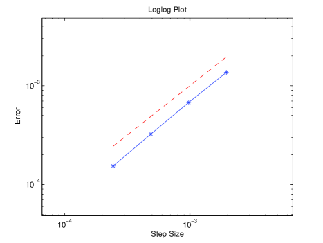
Figure 1: The strong convergence order at the terminal time $T=2$. The red dashed line is the reference line with the slope of 1.

It is interesting to observe from Figure 1 that the strong convergence rate is quite close to one, although we choose $\varepsilon=0.1$ and the theoretical result (4.1) only shows the rate of $0.9$. This observation indicates that our theoretical result is somehow conservative.

We also observe from Theorem 3.7 that the strong convergence rate is highly dependent on the choices of the functions, $\mu(\cdot)$ and $h(\cdot)$. Although we have demonstrated in the example above how to choose them, the example itself has already indicated that those choices may not be optimal.

Moreover, the functions $\mu(\cdot)$ and $h(\cdot)$ are used to set up the truncating barrier $\mu^{-1}(h(\Delta))$. Once the step size is decided, the barrier is set for all states and the whole time interval. To be more efficient, it may be worth to design a current-state-dependent truncating barrier, which then may end up with a numerical method with variable step size. We have been working on this new method and will report it later on.

References

• [1] E. Allen, Modeling with Itô stochastic differential equations, volume 22 of Mathematical Modelling: Theory and Applications. Springer, Dordrecht, 2007.
• [2] B. Oksendal, Stochastic differential equations, An introduction with applications, Universitext. Springer-Verlag, Berlin, sixth edition, 2003.
• [3] X. Mao, Stochastic Differential Equations and Applications, second ed., Horwood, Chichester, 2007.
• [4] P.E. Kloeden, E. Platen, Numerical Solution of Stochastic Differential Equations, Springer-Verlog, Berlin, 1992.
• [5] G.N. Milstein, M.V. Tretyakov, Stochastic Numerics for Mathematical Physics, Springer-Verlag, Berlin, 2004.
• [6] E. Platen, N. Bruti-Liberati, Numerical Solution of Stochastic Differential Equations with Jumps in Finance, Springer-Verlag, Berlin, 2010.
• [7] D.J. Higham, Stochastic ordinary differential equations in applied and computational mathematics, IMA J. Appl. Math., special issue: ”2020 visions of applied mathematics”, 76 (2011) 449-474.
• [8] M. Hutzenthaler, A. Jentzen, P.E. Kloeden, Strong and weak divergence in finite time of Euler’s method for stochastic differential equations with non-globally Lipschitz continuous coefficients, Proc. R. Soc. A 467 (2011) 1563-1576.
• [9] M. Hutzenthaler, A. Jentzen, P.E. Kloeden, Divergence of the multilevel Monte Carlo Euler method for nonlinear stochastic differential equations, Ann. Appl. Probab. 23(5) (2013) 1913-1966.
• [10] G.N. Milstein, E. Platen, H. Schurz, Balanced implicit methods for stiff stochastic system, SIAM J. Numer. Anal. 35 (1998) 1010-1019.
• [11] Y. Hu, Semi-implicit Euler-Maruyama scheme for stiff stochastic equations, Stochastic Analysis and Related Topics, V (Silivri, 1994), 183-202, Progr. Probab., 38, Birkhäuser Boston, Boston, MA, 1996.
• [12] D.J. Higham, X. Mao, A. Stuart, Strong convergence of Euler-type methods for nonlinear stochastic differential equations, SIAM J. Numer. Anal. 40(3) (2002) 1041-1063.
• [13] L. Szpruch, X. Mao, D.J. Higham, J. Pan, Numerical simulation of a strongly nonlinear Ait-Sahalia type interest rate model, BIT 51(2) (2011) 405–425.
• [14] X. Mao, L. Szpruch, Strong convergence rates for backward Euler-Maruyama method for non-linear dissipative-type stochastic differential equations with super-linear diffusion coefficients, Stochastics 85(1) (2013) 144-171.
• [15] A. Neuenkirch, L. Szpruch, First order strong approximations of scalar SDEs defined in a domain, Numer. Math. 128(1) (2014) 103-136.
• [16] C. Yue, C. Huang, F. Jiang, Strong convergence of split-step theta methods for non-autonomous stochastic differential equations, Int. J. Comput. Math. 91(10) (2014) 2260-2275.
• [17] X. Wang, S. Gan, D. Wang, A family of fully implicit Milstein methods for stiff stochastic differential equations with multiplicative noise, BIT 52(2) (2012) 741-772.
• [18] S. Dereich, A. Neuenkirch, L. Szpruch, An Euler-type method for the strong approximation of the Cox-Ingersoll-Ross process, Proc. R. Soc. Lond. Ser. A Math. Phys. Eng. Sci. 468(2140) (2012) 1105-1115.
• [19] K. Burrage, T. Tian, Implicit stochastic Runge-Kutta methods for stochastic differential equations, BIT 44(1) (2004) 21-39.
• [20] S.S. Ahmad , P.N. Chandra, S. Raha, The fully implicit stochastic-$\alpha$ method for stiff stochastic differential equations, J. Comput. Phys. 228(22) (2009) 8263-8282.
• [21] H. Schurz, Basic concepts of numerical analysis of stochastic differential equations explained by balanced implicit theta methods, Stochastic differential equations and processes, Springer Proc. Math. 7, Springer, Heidelberg, 2012, pp. 1-139.
• [22] M. Hutzenthaler, A. Jentzen, P.E. Kloeden, Strong convergence of an explicit numerical method for SDEs with non-globally Lipschitz continuous coefficients, Ann. Appl. Probab. 22(2) (2012) 1611-1641.
• [23] M. Hutzenthaler, A. Jentzen, Numerical approximations of stochastic differential equations with non-globally Lipschitz continuous coefficients, Mem. Amer. Math. Soc. 236(2) (2015) 99 pages.
• [24] S. Sabanis, A note on tamed Euler approximations, Electron. Commun. Probab. 18(47) (2013) 1-10.
• [25] X. Wang, S. Gan, The tamed Milstein method for commutative stochastic differential equations with non-globally Lipschitz continuous coefficients, J. Differ. Equ. Appl. 19(3) (2013) 466-490.
• [26] X. Zong, F. Wu, C. Huang, Convergence and stability of the semi-tamed Euler scheme for stochastic differential equations with non-Lipschitz continuous coefficients, Appl. Math. Comput. 228 (2014) 240-250.
• [27] X. Mao, The truncated Euler–Maruyama method for stochastic differential equations, J. Comput. Appl. Math. 290 (2015) 370-384.
• [28] X. Mao, Convergence rates of the truncated Euler-Maruyama method for stochastic differential equations, J. Comput. Appl. Math. 296 (2016) 362-375.
• [29] Q. Guo, W. Liu, X. Mao, R. Yue, The partially truncated Euler-Maruyama method and its stability and boundedness, Appl. Numer. Math. 115 (2017), 235-251.
• [30] M.B. Giles, Multi-level Monte Carlo path simulation, Oper. Res. 56(3) (2008) 607-617.
• [31] M.B. Giles, Improved multilevel Monte Carlo convergence using the Milstein scheme, Monte Carlo and quasi-Monte Carlo methods 2006, Springer, Berlin, 2008, pp. 343-358.
• [32] G. Milstein, Approximate integration of stochastic differential equations, Theor. Probab. Appl. 19 (1974) 583-588.