Single Image Super-Resolution based on Wiener Filter in Similarity Domain

Abstract

Single image super resolution (SISR) is an ill-posed problem aiming at estimating a plausible high resolution (HR) image from a single low resolution (LR) image. Current state-of-the-art SISR methods are patch-based. They use either external data or internal self-similarity to learn a prior for a HR image. External data based methods utilize large number of patches from the training data, while self-similarity based approaches leverage one or more similar patches from the input image. In this paper we propose a self-similarity based approach that is able to use large groups of similar patches extracted from the input image to solve the SISR problem. We introduce a novel prior leading to collaborative filtering of patch groups in 1D similarity domain and couple it with an iterative back-projection framework. The performance of the proposed algorithm is evaluated on a number of SISR benchmark datasets. Without using any external data, the proposed approach outperforms the current non-CNN based methods on the tested datasets for various scaling factors. On certain datasets, the gain is over 1 dB, when compared to the recent method A+. For high sampling rate (x4) the proposed method performs similarly to very recent state-of-the-art deep convolutional network based approaches.

I Introduction

The goal of single image super-resolution (SISR) is to estimate the high frequency spectrum of an image from a single band limited measurement. In other words, it means generating a plausible high resolution image that does not contradict the low resolution version used as input. It is a classical problem in image processing which finds numerous applications in medical imaging, security, surveillance and astronomical imaging, to name few. Simple methods based on interpolation (e.g., bilinear, bicubic) are frequently employed because of their computational simplicity, but due to use of low order polynomials, they mostly yield very smooth results that do not contain the sharp edges or fine textures, often present in natural images.

In recent years, these shortcomings have been partially resolved by approaches that use machine learning to generate a low resolution (LR) to high resolution (HR) mapping from a large number of images [38, 29]. Existing methods utilized to learn this mapping include manifold learning [4], sparse coding [42], convolutional neural networks (CNNs) [11, 24, 25], and local linear regression [37, 38]. The prior learned by these approaches has been shown to effectively capture natural image structure, however, the improved performance comes with some strong limitations. First, they heavily rely on a large amount of training data, which can be very specific for different kind of images and somehow limits the domain of application. Second, a number of these approaches, most markedly the CNN based ones, take a considerable amount of training time, ranging from several hours to several days on very sophisticated graphical processing unitss (GPUs). Third, a separate LR-HR mapping must be learned for each individual up-sampling factor and scale ratio, limiting its use to applications were these are known beforehand. Finally, a number of these approaches [38, 37], do not support non-integer up-sampling factors.

Certain researchers have addressed the SISR problem by exploiting the priors from the input image in various forms of self-similarity [20], [18], [6], [13]. Freedman and Fattal [18] observed that, although fewer in number, the input image based search results in “more relevant patches”. Some self-similarity based algorithms find a LR-HR pair by searching for the most similar target patch in the down-sampled image [20, 18, 23, 32]. Other approaches are able to use several self-similar patches and couple them with sparsity based approaches, such as Dong et al. [13]. Yang and Wang [44] are also able to self-learn a model for the reconstruction using sparse representation of image patches. Shi and Qi [30] use a low-rank representation of non-local self-similar patches extracted from different scales of the input image. These approaches do not required training or any external data, but their performance is usually inferior to approaches employing external data, especially on natural images with complex structures and low degree of self-similarity. Still, in all of them, sparsity is regarded as an instrumental tool in improving the reconstruction performance over previous attempts.

In this work we propose Wiener filter in Similarity Domain for Super Resolution (WSD-SR), a technique for SISR that simultaneously considers sparsity and consistency. To achieve this aim, we formulate the SISR problem as a minimization of reconstruction error subject to a sparse self-similarity prior. The core of this work lies in the design of the regularizer that enforces sparsity in groups of self-similar patches extracted from the input image. This regularizer, which we term Wiener filter in Similarity Domain (WSD), is based on Block Matching 3D (BM3D) [7, 8], but includes particular twists that make a considerable difference in SISR tasks. The most significant one is the use of a 1D Wiener filter that only operates along the dimension of similar patches. This feature alone, mitigates the blur introduced by the regularizers designed for denoising that make use of 3D filtering and proved essential for the high performance of our proposed method (see Table I).

II Contribution and Structure of the Paper

The main characteristics of the proposed approach are as follows:

1. No external data or training required: the proposed approach exploits the image self-similarity, therefore, it does not require any external data to learn an image prior, nor does it need any training stage;

2. Supports non-integer scaling factors: the image can be scaled by any factor and aspect ratio;

3. No border pruning effect: The proposed approach represents the complete image in the high resolution space without any border pruning effect, unlike most of the dictionary based algorithms [47, 38].

4. Excellent performance: it competes with the state-of-the-art approaches in both computational complexity and estimation quality as will be demonstrated in section VI.

The previous conference publication of the proposed approach was done in [15]. The algorithm in this paper follows the general structure of [15], but introduces a novel regularizer that proved crucial for obtaining significantly improved performance. The distinctive features of the developed algorithm are:

• 1D Wiener filtering along similarity domain;

• Reuse of grouping information;

• Adaptive search window size;

• Iterative procedure guided by input dependent heuristics;

• Improved parameter tuning.

An extensive simulation study demonstrates the advanced performance of the developed algorithm as compared with [15] and some state-of-the-art methods in the field.

The paper is organized as follows. In Section III we provide an overview of modern single image super-resolution methods. In Section IV we formulate the problem and present the framework we used to solve it. Section V contains the main contribution of this paper and provides a detailed exposition and analysis of the novel regularizer to be employed within the presented framework. Section VI provides an experimental analysis of our proposal and comparison against several other SISR methods, both quantitative and qualitative. Section VII analyses possible variations of the proposed approach that could lead to further improvements. Finally, Section VIII provides a summary of the work.

III Related Work

The SISR algorithms can be broadly divided into two main classes: the methods that rely solely on observed data and those that additionally use external data. Both of these classes can be further divided into the following categories: learning-based and reconstruction-based. However, we are going to present below the related work in a simplified division of the methods that only accounts for use, or lack of use, of external data without any aim to be considered as an extensive review of the field.

III-A Approaches Using External Data

This type of approaches use a set of HR images and their down-sampled LR versions to learn dictionaries, regression functions or end-to-end mapping between the two. Initial dictionary-based techniques created a correspondence map between features of LR patches and a single HR patch [19]. Searching in this type of dictionaries was performed using approximate nearest neighbours (ANN), as exhaustive search would be prohibitively expensive. Still, dictionaries quickly grew in size with the amount of used training data. Chang et al. [4] proposed the use of locally linear embedding (LLE) to better generalize over the training data and therefore require smaller dictionaries. Image patches were assumed to live in a low dimensional manifold which allowed the estimation of high resolution patches as a linear combination of multiple nearby patches. Yang et al. [42] also tackled to problem of growing dictionary sizes, but using sparse coding. In this case, a technique to obtain a sparse “compact dictionary” from the training data is proposed. This dictionary is then used to find a sparse activation vector for a given LR patch. The HR estimate is finally obtained by multiplying the activation vector by the HR dictionary. Yang et al. [43], Zeyde et al. [47] build on this approach and propose methods to learn more compact dictionaries. Ahmed and Shah [1] learns multiple dictionaries, each containing features along a different direction. The high-resolution patch is reconstructed using the dictionary that yields the lowest sparse reconstruction error. Kim and Kim [26] does away with the expensive search procedure by using a new feature transform that is able to perform simultaneous feature extraction and nearest neighbour identification. Dictionaries can also be leveraged together with regression based techniques to compute projection matrices that, when applied to the LR patches, produce a HR result. The papers by Timofte et al. [37, 38, 39] are examples of such an approach where for each dictionary atom, a projection matrix that uses only the nearest atoms is computed. Reconstruction is performed by finding the nearest neighbour of the LR patch and employing the corresponding projection matrix. Zhang et al. [48] follows a similar approach but also learns the clustering function, reducing the required amount of anchor points. Other approaches do not build dictionaries out of the training data, but chose to learn simple operators, with the advantage of creating more computationally efficient solutions. Tang and Shao [36] learns two small matrices that are used on image patches as left and right multiplication operator and allow fast recovery of the high resolution image. The global nature of these matrices, however, fails to capture small details and complex textures. Choi and Kim [5] learns instead multiple local linear mappings and a global regressor, which are applied in sequence to enforce both local and global consistency, resulting in better representation of local structure. Sun et al. [35] learns a prior and applies it using a conventional image restoration approach. Finally, neural networks have also been explored to solve this problem, in various ways. Sidike et al. [31] uses a neural network to learn a regressor that tries to follow edges. Zeng et al. [46] proposes the use of coupled deep autoencoder (CDA) to learn both efficient representations for low and high resolution patches as well as a mapping function between them. However, a more common use of this type of computational model is to leverage massive amounts of training data and learn a direct low to high resolution image mapping [12, 27, 24, 25]. Of these approaches, only Liu et al. [27] tries to include domain expertise in the design phase, and despite the fact that testing is relatively inexpensive, training can take days even on powerful computers.

Although these approaches learn a strong prior from the large amount of training data, they require a long time to train the models. Furthermore, a separate dictionary is trained for each up-sampling factor, which limits the available up-sampling factors during the test time.

III-B Approaches Based Only on Observed Data

This type of approaches rely on image priors to generate an HR image having only access to the LR observation. Early techniques of this sort are still heavily used due to their computational simplicity, but the low order signal models that they employ fail to generate the missing high frequency components, resulting in over-smoothed estimates. Haris et al. [22] manages to partially solve this problem by using linear interpolators that operate only along the edge direction. Wei and Dragotti [41] explores the use finite rate of innovation (FRI) to enhance linear up-scaling techniques with piece-wise polynomial estimates. Other solutions use separate models for the low-frequency and high-frequency components, the smooth areas and the textures and edges [10, 45]. An alternative approach to image modeling draws from the concept of self-similarity, the idea that natural images exhibit high degree of repetitive behavior. Ebrahimi and Vrscay [14] proposed a super-resolution algorithm by exploiting the self-similarity and the fractal characteristic of the image at different scales, where the non-local means [3] is used to perform the weighting of patches. Freedman and Fattal [18] extended the idea by imposing a limit on the search space and, thereby, reduced the complexity. They also incorporated incremental up-sampling to obtain the desired image size. Suetake et al. [34] utilized the self-similarity to generate an example code-book to estimate the missing high-frequency band and combined it with a framework similar to [19]. Glasner et al. [20] used self-examples within and across multiple image scales to regularize the otherwise ill-posed classical super-resolution scheme. Singh et al. [33] proposed an approach for super-resolving the image in the noisy scenarios. Egiazarian and Katkovnik [15], introduced the sparse coding in the transform domain to collectively restore the local structure in the high resolution image. Dong et al. [13] also employs self-similarity to model each pixel as a linear combination of its non-local neighbors. Cui et al. [6] utilized the self-similarity with a cascaded network to incrementally increase the image resolution. Recently, Huang et al. [23] improved the search strategy by considering affine transformations, instead of translations, for the best patch match. Further, various search strategies have been proposed to improve the LR-HR pair based on textural pattern [32], optical flow [49] and geometry [17].

IV Framework for Iterative SISR

A linear ill-posed inverse problem, typical for image restoration, in particular, for image deblurring and super-resolution, is considered here for the noiseless case:

$$\bm{y}=\bm{Hx}$$ (1)

where $\bm{y}\in\mathbb{R}^{m}$, $\bm{x}\in\mathbb{R}^{n}$, $m\leq n$, $\bm{H}$ is a known linear operator.

The problem is to solve (1) with respect to $\bm{x}$ provided some prior information on $\bm{x}$. In terms of super-resolution, the operations in $\mathbb{R}^{m}$ and $\mathbb{R}^{n}$ can be treated as operations with low- and high-resolution images, respectively. Iterative algorithms to estimate $\bm{x}$ from (1) usually include both up-sampling and down-sampling operations along with some prior information on these variables.

In this work we solve this inverse problem using a general approach similar to one introduced in Danielyan et al. [9] for image deblurring, but focusing on the specific problem of SISR.

The sparse reconstruction of $\bm{x}$ can be formulated as the following constrained optimization:

$$\min_{\bm{\theta}\in\mathbb{R}^{m}}\text{ }||\bm{\theta}||_{0}\text{, }||\bm{y}-\bm{Hx||}_{2}^{2}\leq\varepsilon^{2}\text{,}$$ (2)

$$\text{ }\bm{x}=\bm{\Psi\theta}\text{, }\bm{\theta=\Phi x}.$$

Here $\bm{\Phi}\in\mathbb{R}^{m\times n}$ and $\bm{\Psi}\in\mathbb{R}^{n\times m}$ are analysis and syntheses matrices, $\bm{\theta}\in\mathbb{R}^{m}$ is a spectrum vector, and $\varepsilon$ is a parameter controlling the accuracy of the equation (1). For the super-resolution problem $m<n$. Recall that $l_{0}$-pseudo norm, $||\bm{\theta}||_{0}$, is calculated as a number of non-zero elements of $\bm{\theta}$ and $||.||_{2}$ denotes the $l_{2}$ norm.

Sparse reconstruction of $\bm{x}$ means minimization of $||\bm{\theta}||_{0}$ corresponding to a sparse representation for $\bm{x}$ provided equations linking the image with the spectrum and the inequality defining the accuracy of the observation fitting. While the straightforward minimization (2) is possible, our approach is essentially different. Following Danielyan et al. [9], we apply the multiple-criteria Nash equilibrium technique using the following two cost functions:

$$J_{1}(\bm{\theta,x})=\frac{1}{2\varepsilon^{2}}||\bm{y}-\bm{Hx}||_{2}^{2}+\frac{1}{2\gamma}||\bm{x}-\bm{\Psi\theta}||_{2}^{2},$$ (3)

$$J_{2}(\bm{\theta,x})=\frac{1}{2}||\bm{\theta}-\bm{\Phi x}||_{2}^{2}+\tau_{\theta}||\bm{\theta}||_{0}.$$ (4)

The first summand in $J_{1}$ corresponds to the given observations  and the second one is penalization of the equation $\bm{x}=\bm{\Psi\theta}$. The criterion $J_{2}$ enables the sparsity of the spectrum $\bm{\theta}$ for $\bm{x}$ provided the restriction $\bm{\theta=\Phi x}$. The Nash equilibrium for (3)-(4) is a consensus of restrictions imposed by $J_{1}$, $J_{2}$. It is defined as a fixed point ($\bm{\theta}^{\ast}$, $\bm{x}^{\ast}$) such that:

$$\bm{x}^{\ast} = \arg\min_{\bm{x}}J_{1}(\bm{\theta}^{\ast},\bm{x})\text{,}$$ (5)

$$\bm{\theta}^{\ast} = \arg\min_{\bm{\theta}}J_{2}(\bm{\theta,x}^{\ast})\text{.}$$ (6)

The equilibrium ($\bm{\theta}^{\ast}$, $\bm{x}^{\ast}$) means that any deviation from this fixed point results in increasing of at least one of the criteria.

The iterative algorithm looking for the fixed point has the following typical iterative form [16]:

$$\bm{x}^{k+1} = \arg\min_{\bm{x}}J_{1}(\bm{\theta}^{k},\bm{x})\text{,}$$ (7)

$$\bm{\theta}^{k+1} = \arg\min_{\bm{\theta}}J_{2}(\bm{\theta,x}^{k+1})\text{.}$$ (8)

We modify this procedure by replacing the minimization of $J_{1}$ on $\bm{x}$ by a gradient descent step corresponding to the gradient

$$\partial J_{1}/\partial\bm{x}=\frac{1}{\varepsilon^{2}}\bm{H}^{T}(\bm{y}-\bm{Hx})-\frac{1}{\gamma}(\bm{x}-\bm{\Psi\theta})\text{.}$$ (9)

Accompanied by minimization of $J_{2}$ on $\bm{\theta}$ it gives the following iterations for the solution of the problem at hand:

$$\bm{x}^{k+1} = \bm{\tilde{x}}^{k}$$

$$+\>\alpha(\bm{H}^{T}\bm{H})^{+}\left[\frac{1}{\varepsilon^{2}}\bm{H}^{T}(\bm{y}-\bm{H\tilde{x}}^{k})-\frac{1}{\gamma}(\bm{x}^{k}-\bm{\tilde{x}}^{k})\right],$$

$$\bm{\theta}^{k+1} = \arg\min_{\bm{\theta}}J_{2}(\bm{\theta,x}^{k+1}),$$ (11)

$$\bm{\tilde{x}}^{k+1} = \bm{\Psi\theta}^{k+1}.$$ (12)

Here (⁺) stands for the Moore-Penrose pseudo-inverse. The matrix $(\bm{H}^{T}\bm{H})^{+}$ is a typical factor used for acceleration of the gradient iterations.

The optimization on $\bm{\theta}$ in (11) gives as a solution the hard-thresholding (HT) with the threshold equal to $\sqrt{2\tau_{\theta}}$, where $\tau_{\theta}$ denotes the threshold parameter such that:

$$\bm{\theta}^{k}=Th_{\sqrt{2\tau_{\theta}}}(\bm{\Phi x}^{k})\text{.}$$ (13)

This thresholded spectrum combined the with the equality $\bm{\tilde{x}}^{k}=\bm{\Psi\theta}^{k}$ defines the filter with input $\bm{x}^{k}$, output $\bm{\tilde{x}}^{k}$ and threshold parameter $\tau_{\theta}$:

$$\bm{\tilde{x}}^{k}=\mathcal{F}_{1}(\bm{x}^{k},\tau_{\theta})\text{.}$$ (14)

Then the algorithm can be written in the following compact form

$$\bm{x}^{k+1} = \bm{\tilde{x}}^{k}$$

$$+\>\alpha(\bm{H}^{T}\bm{H})^{+}\left[\bm{H}^{T}(\bm{y}-\bm{H\tilde{x}}^{k})\frac{1}{\varepsilon^{2}}-\frac{1}{\gamma}(\bm{\tilde{x}}^{k}-\bm{x}^{k})\right],$$

$$\bm{\tilde{x}}^{k+1} = \mathcal{F}_{1}(\bm{x}^{k+1},\tau_{\theta}).$$ (16)

The first line of this algorithm defines an update of the super-resolution image $\bm{x}^{k+1}$ obtained from the low resolution residue $\bm{y}-\bm{H\tilde{x}}^{k}$. Note, that $(\bm{H}^{T}\bm{H})^{+}\bm{H}^{T}\in\mathbb{R}^{n\times m}$ is an up-sampling operator (matrix), which we will denote by $\bm{U}\in\mathbb{R}^{n\times m}$:

$$\bm{U}=(\bm{H}^{T}\bm{H})^{+}\bm{H}^{T}.$$ (17)

The last summand $(\bm{\tilde{x}}^{k}-\bm{x}^{k})/\gamma$ in (IV) is the scaled difference between the image estimate after and before filtering. Experiments show that this summand is negligible. Dropping this term, replacing $\alpha/\varepsilon^{2}$ by $\alpha$ and exchanging the order of the operations (IV) and (16) we arrive to the simplified version of the algorithm:

$$\bm{\tilde{x}}^{k} = \mathcal{F}_{1}(\bm{x}^{k-1},\tau_{\theta}),$$ (18)

$$\bm{x}^{k} = \bm{\tilde{x}}^{k}+\alpha\bm{U}(\bm{y}-\bm{H\tilde{x}}^{k}).$$ (19)

The filter $\mathcal{F}_{1}$ is completely defined by the used analysis and synthesis operators $\bm{\Phi}\in\mathbb{R}^{m\times n}$ and $\bm{\Psi}\in\mathbb{R}^{n\times m}$. In particular, if the BM3D block-matching is used for design of the analysis and synthesis operators, the filter $\mathcal{F}_{1}$ is the BM3D HT algorithm (see Danielyan et al. [9]).

We replaced this BM3D HT algorithm by our proposed regularizer WSD, which uses the BM3D grouping but is especially tailored for super-resolution problems.

The algorithm takes now the final form, which is used in our demonstrative experiments:

$$\bm{\tilde{x}}^{k} = \text{WSD}(\bm{x}^{k-1},\tau^{k}_{\theta}),$$ (20)

$$\bm{x}^{k} = \bm{\tilde{x}}^{k}+\alpha\bm{U}(\bm{y}-\bm{H\tilde{x}}^{k})\text{.}$$ (21)

This proposed iterative algorithm is termed WSD-SR, and formally described in Procedure 1.

Procedure 1 WSD-SR algorithm

0:  $y$: low resolution input

0:  $H$: sampling operator

0:  $K$: number of iterations

0:  High resolution estimate

1:  $U=(H^{T}H)^{+}H^{T}$ {up-sampling matrix}

2:  $x^{0}=Uy$ {initial estimate}

3:  for $k=1$ to K do

4:     $\tilde{x}^{k}$ = WSD($x^{k-1}$, $\tau_{\theta}^{k}$)

5:     $x^{k}=\alpha U(y-H\tilde{x}^{k})+\tilde{x}^{k}$

6:  end for

7:  return  $x^{K}$

Note, that (20) defines the regularizing stage of the super-resolution algorithm. The analysis and synthesis transforms used in WSD are data dependent and, as a result, vary from iteration-to-iteration, as in BM3D. The parameter $\tau_{\theta}$ is also changing throughout the iterations, in order to account for the need to reduce the strength of the regularizer in the later stages of the iterative procedure.

V Proposed Regularizer

Figure 1: WSD block diagram.

The proposed regularizer, WSD, is highly influenced by the BM3D collaborative filtering scheme that explores self-similarity of natural images [8].

Procedure 2 WSD algorithm

0:  $x$: filter input

0:  $\tau_{\theta}$: filter strength

0:  $K^{pilot}$: pilot recompute period

0:  $k$: current iteration

0:  $\tilde{x}$: estimate {Compute match table for pilot estimation.}

1:  if $k=0$ then

2:     $m^{ht}\leftarrow$ HTBlockMatch $(x)$

3:  else

4:     $m^{ht}\leftarrow m^{ht}_{previous}$

5:  end if

6:  

7:   {Pilot estimation.}

8:  if $k\mod K^{pilot}=0$ then

9:     $g^{ht}\leftarrow$ Group $(x,m^{ht})$

10:     $\tilde{g}^{ht}\leftarrow$ HardThresholding $(g^{ht},\tau_{\theta})$

11:     $\tilde{x}^{pilot}\leftarrow$ Aggregate $(\tilde{g}^{ht})$

12:     $m^{pilot}\leftarrow$ WienerBlockMatch $(\tilde{x}^{pilot})$

13:  else

14:     $\tilde{x}^{pilot}\leftarrow\tilde{x}^{pilot}_{previous}$

15:     $m^{pilot}\leftarrow m^{pilot}_{previous}$

16:  end if

17:  

18:   {Filter the input image using pilot information.}

19:  $g^{pilot}\leftarrow$ Group $(\tilde{x}^{pilot},m^{pilot})$

20:  $W\leftarrow$ EstimateWiener $(g^{pilot},\tau_{\theta})$

21:  $g^{wiener}\leftarrow$ Group $(x,m^{pilot})$

22:  $\tilde{g}^{wiener}\leftarrow$ WienerFilter $(g^{wiener},W)$

23:  $\tilde{x}\leftarrow$ Aggregate $(\tilde{g}^{wiener})$

24:  

25:   {Store information for future reuse.}

26:  $m^{ht}_{previous}\leftarrow m^{ht}$

27:  $\tilde{x}^{pilot}_{previous}\leftarrow\tilde{x}^{pilot}$

28:  $m^{pilot}_{previous}\leftarrow m^{pilot}$

29:  

30:  return  $\tilde{x}$

As shown in Fig. 1 and further described in Procedure 2, WSD operates in two sequential stages, both filtering groups of similar patches, as measured using the Euclidean distance. The result of each stage is created by placing the filtered patches back in their original locations and performing simple average for pixels with more than one estimate. The two stages employ different filters on the patch groups. The first stage, which is producing a pilot estimate used by the second stage, uses HT in the 3D transform domain. The second stage on the other hand, which is generating the final result, uses the result of the first stage to estimate an empirical Wiener filter in the 1D transform domain, operating only along the inter-patch dimension, which we call the similarity domain. This filter is then applied to the original input data.

The use of the 1D Wiener filter in the second stage sets this approach apart from both Egiazarian and Katkovnik [15] and Wang et al. [40]. It allowed to not only achieve much sharper results and clearer details, but also reduce the computational cost. Furthermore, the employed grouping procedure includes two particular design elements that further improved the system’s performance and reduced its computational complexity: reuse of block match results and adaptive search window size. Finally, as described in the previous section, WSD is applied iteratively in what we term WSD-SR. This requires the modulation of the filtering strength in such a way that it is successively decreased as the steady-state is approached, in a sort of simulated annealing fashion [21]. We present input dependent heuristics for the selection of both the minimum number of iterations and the filter strength curve.

Overall, the main features of our proposal are:

1. Wiener filter in similarity domain;

2. stateful operation with grouping information reuse;

3. adaptive search window size;

4. input dependent iterative procedure parameters.

These design decisions, as well as the parameters selection are studied in this section. Empirical evidence is presented for each decision, both in terms of reconstruction quality (PSNR) and computational complexity (speed-up factor). The tests were conducted on Set5 [2] using a scale factor of $4$, and sampling operator $H$ set to bicubic interpolation with anti-aliasing filter. In all tables, only the feature under analysis changes between the different columns and the column marked with a * reflects the final design.

V-A Wiener Filter in Similarity Domain

The original work on collaborative filtering [8] addresses the problem of image denoising, hence, exploits not only the correlation between similar patches but also between pixels of the same patch. It does so by performing 3D Wiener filtering on groups of similar patches. The spectrum of each group is computed by a separable 3D transform composed of a 2D spatial transform $T_{2D}$ and a 1D transform $T_{1D}$ along the similarity dimension. However, when dealing with the problem of noiseless super-resolution, employing a 3D Wiener filter results in spatial smoothing, which is further exacerbated by the iterative nature of the algorithm. In order to avoid this problem we use $T_{2D}=I$, which means performing 1D Wiener filtering along the inter-patch similarity dimension. More specifically, given a match table $m$, a pilot estimate $\tilde{x}^{pilot}$, and an operation $x(:,m)$ that extracts from $x$ the patches addressed by $m$ as columns, a 1D empirical Wiener filter $W$ of strength $\tau_{theta}$ is estimated as follows:

$$\bm{g}^{pilot} = \tilde{\bm{x}}^{pilot}(:,m)$$ (22)

$$\bm{G}^{pilot} = \bm{g}^{pilot}\bm{T}_{1D}$$ (23)

$$\bm{W} = \frac{|\bm{G}^{pilot}|^{2}}{(|\bm{G}^{pilot}|^{2}+\tau_{theta}^{2})}$$ (24)

The filter is applied by performing point-wise multiplication with the spectrum of the group of similar patches extracted from the input image $x$, using the same match table $m$ that was used to estimate the Wiener coefficients $W$:

$$\bm{g}^{wiener} = \bm{x}(:,m)$$ (25)

$$\bm{G}^{wiener} = \bm{g}^{wiener}\bm{T}_{1D}$$ (26)

$$\tilde{\bm{G}}^{wiener} = \bm{W}.*\bm{G}^{wiener}$$ (27)

$$\tilde{\bm{g}}^{wiener} = \bm{T}^{-1}_{1D}\tilde{\bm{G}}^{wiener}$$ (28)

The resulting filtered group of patches $\tilde{\bm{g}}^{wiener}$ is ready to be aggregated.

These operations are presented in Procedure 2 using symbolic names. There, the Group() operation stands for $x(:,m)$, EstimateWiener() stands for equations (23)-(24) and WienerFilter() stands for equations (26)-(28).

Besides dramatically improving the reconstruction quality, this feature significantly reduces the computational complexity of WSD when compared to a 3D transform based approach, as suggested by the empirical evidence in Table I.

TABLE I: Wiener filter in similarity domain effect on performance (Set5, x4), using Haar transform as $T_{1D}$. Speedup is a factor relative to $T_{2D}^{wiener}$ = DCT.

$T^{2D}_{Wiener}$	DCT	Identity*
	PSNR	PSNR	Speedup
Baby	$33.48$	$33.55$	$1.73$
Bird	$32.74$	$33.25$	$1.68$
Butterfly	$24.26$	$27.45$	$1.54$
Head	$32.57$	$32.65$	$1.68$
Woman	$28.67$	$30.04$	$1.69$
Average	$30.35$	$31.39$	$1.66$

V-B Grouping Information Reuse

In the proposed approach, we apply collaborative filtering iteratively on the input image. However, because the structure of the image does not change significantly between iterations, the set of similar patches remains fairly constant. Therefore, we decided to perform block matching sparsely and reuse the match tables. We observed that in doing so, we not only gain in terms of reduced computational complexity, but also in terms of reconstruction quality. We speculate that the improved performance stems from the fact that by using a set of similar patches for several iterations we avoid oscillations between local minima, and by revising it sporadically, we allow for small structural changes that reflect the contribution of the estimated high frequencies.

Each iteration of the collaborative filter typically requires the execution of the grouping procedure twice, the first time to generate the grouping for HT and the second one to generate the grouping for Wiener filtering. We observed that this iterative procedure is fairly robust to small changes on the grouping used for the HT stage, to the point that optimal results are achieved when that match table is computed only once. The same is not true for the Wiener stage’s match table, which still needs to be computed every few iterations, $K^{pilot}$ in Procedure 2. Table II presents the empirical evidence concerning these observations.

TABLE II: Match table reuse effect on performance (Set5, x4). $K^{pilot}=5$. Speedup is a factor relative to match table reuse: disabled.

Match table reuse	Disabled	Enabled*
	PSNR	PSNR	Speedup
Baby	$33.50$	$33.55$	$2.82$
Bird	$33.12$	$33.25$	$3.01$
Butterfly	$27.25$	$27.45$	$3.23$
Head	$32.66$	$32.65$	$2.92$
Woman	$29.98$	$30.04$	$3.14$
Average	$31.30$	$31.39$	$3.02$

V-C Adaptive Search Window Size

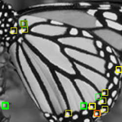
(a) Global

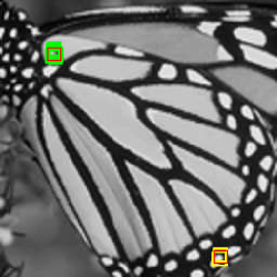
(b) Local

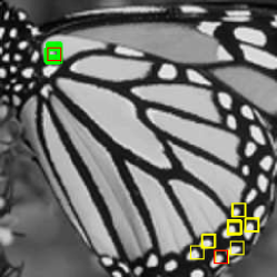
(c) Incremental

Figure 2: Three types of search strategies. Global, local and incremental. Red blocks indicate the reference patches. Green patches denote the matching patches for the reference patch at the top of the butterfly. Yellow patches denote the matching results corresponding to the reference at the bottom of the butterfly.

A straightforward solution to define the search window size for block matching would be to use the whole image as the search space. In doing so, we would be in the situation of global self-similarity and guarantee the selection of all the available patches meeting the similarity constraint. There are, however, two drawbacks to this solution. First, it incurs a significant computational overhead as the complexity grows quadratically with the radius of the search window. Second, it inevitably results in the inclusion of certain patches that, although close to the reference patch in the Euclidean space, represent very different structures in the image. This effect can be observed in Fig. 2a, specifically on the top patch, where global self-similarity results in the selection of patches which do not lie on the butterfly and have very different surrounding structure compared to the reference patch. An alternative solution would be limit the search window to a small neighborhood of the reference patch. However, if the search window is too small, it might happen that not enough similar patches can be found, as exemplified in Fig. 2b. In our proposal we use an incremental approach that starts with a small search window and enlarges it just enough to find a full group of patches which exhibit an Euclidean distance to the reference patch smaller that a preset value. Fig. 2c shows an example where this incremental strategy finds similar patches from the local region for both reference blocks.

We tested the three different definitions of the search space here discussed, aiming to find $32$ similar patches, resulting in Table III. It can can be observed that for some images, the use of global search results in a drop of performance, while the use of incremental search never compromises the reconstruction quality.

TABLE III: Search strategy effect on performance (Set5 x4). Run-time is a factor relative to search strategy: global.

Search Strategy	Global	Local		Incremental*
	PSNR	PSNR	Speedup	PSNR	Speedup
Baby	$33.55$	$33.55$	$19.82$	$33.55$	$20.24$
Bird	$32.79$	$33.25$	$6.73$	$33.25$	$6.70$
Butterfly	$26.97$	$27.06$	$5.37$	$27.45$	$4.89$
Head	$32.57$	$32.66$	$6.14$	$32.65$	$6.15$
Woman	$29.77$	$29.92$	$6.19$	$30.04$	$6.11$
Average	$31.13$	$31.29$	$10.01$	$31.39$	$9.78$

V-D Iterative Procedure Parameters

(a) PSNR plot

(b) Bird

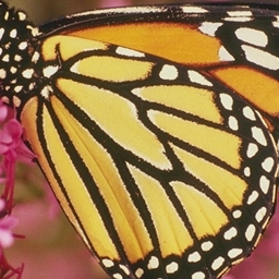
(c) Butterfly

Figure 3: Evolution of algorithm for different images. (a) The PSNR is computed for different number of iterations for two images (bird and butterfly) from Set5. The algorithm progresses quickly for bird while for butterfly it requires more iterations. (b) Bird image has uniform regions and green textured regions, hence also evolves quickly. (c) Butterfly image has sharp edges which results in slow progression.

The iterative nature of the proposed solution introduces the need to select two global parameters that significantly affect the overall system performance: the total number of iterations and the collaborative filter strength curve, $\tau_{\theta}$. We use an inverse square filter strength curve, with fixed starting and end point, as described in the following equation:

$$\tau_{\theta}^{k}=\gamma_{k}\frac{(K-k)}{K}^{2}+\gamma_{s}s$$ (29)

Here $K$ is the total number of iterations, $k$ is the current iteration and $s$ is the scale factor. This curve will lead to slower convergence when more iterations are used and vice-versa, allowing the number of iterations to be adjusted freely.

In order to devise a rule for the selection of the number of iterations, we studied the convergence of the method by reconstruction various images of Set5 using a different number of iterations. Figure 3 shows the results for the bird and butterfly images. These two images have a very different type of content, and the reconstruction of the sharp edges presented by the butterfly image requires a much slower variation of the filtering strength, and therefore many more iterations, than the reconstruction of the more smooth bird image. We speculate that this behavior stems from the low pass nature of the employed sampling operator $H$ and devised a heuristic that uses this known operator to compute the required number of iterations for a particular image. This heuristic is presented together with other implementation details in VI-B, more specifically equation (30).

VI Experiments

Figure 4: Visual comparison with other approaches on the ppt image of Set14, scale factor 4.

Figure 5: Visual comparison with other approaches on the 004 image of Urban100, scale factor 4.

We evaluate the performance of the proposed WSD-SR on three different datasets and three scaling factors. First, we provide details on the datasets, performance evaluation procedure and algorithm implementation. Next, the selected parameters of the proposed method are presented. Then, the performance of the proposed approach is compared with the state-of-the-art techniques, both quantitatively and qualitatively.

All the experiments were conducted on a computer with an Intel Core i7-4870HQ@2.5GHz, 16GB of RAM and an NVIDIA GeForce GT 750M. The WSD-SR implementation used to generate these results can be accessed in the website: http://www.cs.tut.fi/sgn/imaging/sr/wsd/.

VI-A Experimental Setup

Datasets: Following the recent work on SISR, we test our approach on three publicly available datasets. Set5 [2] and Set14 [47] containing 5 and 14 images, respectively. These two datasets have been extensively used by researchers to test super-resolution algorithms, but are quite limited in both the amount and type of images, containing mostly objects and people. For a more thorough analysis we also test the proposed algorithm on the Urban100 dataset proposed by [23] which contains 100 images, including buildings and real world structures.

Performance evaluation: In order to evaluate the performance of the proposed method we use a similar approach as Timofte et al. [38]. Color images are converted to the YCbCr domain and only the luminance channel (Y) is processed and evaluated. The color components, are taken into account for display purposes alone, for which a bicubic interpolation is performed. The evaluation of a method’s performance using a scaling factor of $s$ on an image $z_{orig}$, comprises the following steps:

1. Set $z$ to the luminance channel of $z_{orig}$, which on color images corresponds to the Y component of the YCbCr color transform;

2. Remove columns (on the right) and rows (on the bottom) from $z$ as needed to obtain an image which size is a multiple of $s$ on both width and height, designated $z_{gt}$;

3. Quantize $z_{gt}$ using 8 bit resolution.

4. Generate a low resolution image for processing by down-sampling $z_{gt}$ by a factor of $s$, using bicubic interpolation and an anti-aliasing filter, obtaining $z_{lr}$;

5. Quantize $z_{lr}$ using 8 bit resolution;

6. Super resolve $z_{lr}$, obtaining $y$;

7. Quantize $y$ using 8 bit resolution;

8. Remove a border of $s$ pixels from both $z_{gt}$ and $y$ obtaining $z_{gt\_trimmed}$ and $y_{trimmed}$;

9. Compute the peak signal to noise ratio (PSNR) of $y_{trimmed}$ using as reference $z_{gt\_trimmed}$.

We note that the trimming operations 2 and 8 are done in order to allow for fair comparison with other methods. The proposed method can use any positive real scaling factor and does not generate artefacts at the borders. The quantization operations 3, 5 and 7 are used in order to effectively simulate a realistic scenario where images are usually transmitted and displayed with 8 bit resolution.

VI-B Parameters

The WSD-SR parameters, affecting both WSD and the back projection scheme used throughout these experiments are presented in Table IV, where $s$ stands for the scale factor. Block size $N_{1}$ is an important factor involved in the collaborative filtering which depends on the up-sampling factor. The initial radius of the search window, $N_{S}$, is set to $12$ for both steps. However, the HT step uses only local search, while the Wiener filter stage uses adaptive window size. This difference is evident in the maximum search radius $N_{S_{max}}$. The maximum number of used similar matches, $N_{2}$, is the same for both stages. The regular grid used to select the reference blocks has step size, $N_{step}$, defined such that there is $1$ pixel overlap between adjacent blocks. Finally, the used transforms reflect the main goal of this work, that is, to perform the Wiener filter only along the similarity domain. The total number of iterations is computed using the following heuristic:

$$K=\beta_{1}*\frac{||y-HUy||^{2}_{2}}{m}+\beta_{0}$$ (30)

where $U$ is the up-sampling operator matrix, and $m$ the dimensionality of $y$, both as defined in section IV. This will lead to the use of more iterations in images that are more affected by the sampling procedure. There is however an upper bound of $400$ iterations.

TABLE IV: Proposed WSD-SR parameters.

HT stage parameters	$N^{ht}_{1}$	$max(8,4*(s-1))$
	$N^{ht}_{2}$	$32$
	$N^{ht}_{S_{0}}$	$12$
	$N^{ht}_{S_{max}}$	$12$
	$N^{ht}_{step}$	$N^{ht}_{1}-1$
	$T^{ht}_{2D}$	2D-DCT
	$T^{ht}_{1D}$	1D-Haar
Wiener stage parameters	$N^{wiener}_{1}$	$0.5N^{ht}_{1}$
	$N^{wiener}_{2}$	$32$
	$N^{wiener}_{S_{0}}$	$12$
	$N^{wiener}_{S_{max}}$	$48$
	$N^{wiener}_{step}$	$N^{wiener}_{1}-1$
	$T^{wiener}_{2D}$	$I$
	$T^{wiener}_{1D}$	1D-Haar
Global parameters	$\alpha$	$1.75$
	$\gamma_{k}$	$12$
	$\gamma_{s}$	$2/3$
	$\beta_{1}$	$40/\sqrt{s}$
	$\beta_{0}$	$20$
	$K^{pilot}$	$5$

VI-C Comparison with State-of-the-art

The performance of the proposed approach is compared with several other methods on the already mentioned datasets, using three up-sampling factors $s={2,3,4}$. The results of the proposed approach are compared with the classic bicubic interpolation, the regression based method A+ [38], the random forest based methods ARFL+ [29] and NBSRF [28], the CNN based methods VDSR [24] and DRCN [25] and finally the only self similarity based method on this list, SelfEx [23]. Furthermore, to highlight the importance of using 1D Wiener in the second stage, we also present the quantitative results achieved by our proposal when $T^{wiener}_{2D}=$ 2D-DCT, designated WSD-SR-DCT in Table V. PSNR is used as the evaluation metric and the experimental procedure earlier explained is used for all methods, with the notable exception of VDSR and DRCN for which the PSNR was computed on the publicly available results (only steps 7 to 9 of the experimental procedure).

VI-C1 Quantitative Analysis

TABLE V: The comparison of performance on Set5, Set14 and Urban100.

Dataset	Factor	Bicubic	A+	SelfEx	ARFL+	NBSRF	VDSR	DRCN	WSD-SR-DCT	WSD-SR
Set5	$2$	$33.68$	$36.58$	$36.57$	$36.58$	$36.76$	$37.53$	$37.63$	$36.54$	$37.21$
	$3$	$30.41$	$32.60$	$32.63$	$32.46$	$32.75$	$33.67$	$33.83$	$32.69$	$33.50$
	$4$	$28.43$	$30.30$	$30.31$	$30.15$	$30.44$	$31.35$	$31.54$	$30.39$	$31.39$
Set14	$2$	$30.24$	$32.29$	$32.37$	$32.26$	$32.44$	$33.05$	$33.06$	$32.39$	$32.83$
	$3$	$27.54$	$29.13$	$29.24$	$29.04$	$29.25$	$29.78$	$29.77$	$29.26$	$29.72$
	$4$	$26.00$	$27.32$	$27.47$	$27.23$	$27.41$	$28.02$	$28.02$	$27.43$	$27.98$
Urban100	$2$	$26.88$	$29.24$	$29.56$	$29.13$	$29.45$	$30.77$	$30.76$	$29.39$	$30.29$
	$3$	$24.46$	$26.05$	$26.45$	$25.87$	$26.18$	$27.14$	$27.15$	$26.18$	$26.95$
	$4$	$23.14$	$24.34$	$24.79$	$24.19$	$24.44$	$25.19$	$25.14$	$24.46$	$25.16$

Table V shows the quantitative results of these methods. It can be observed that the proposed approach outperforms all but the more recent CNN based methods: VDSR and DRCN. Note that these two methods used external data and reportedly require 4 hours and 6 days to generate the necessary models, contrary to our approach that relies solely on the image data. Comparing to the only other self-similarity based method, SelfEx [23], the proposed method shows considerable better performance, implying that the collaborative processing of the mutually similar patches provides a much stronger prior than the single most similar patch from the input image. We also note that for high up-sampling factors of Urban100, the performance of the proposed method is in par with even the CNN based methods, showing that this approach is especially suited for images with a high number of edges and marked self-similarity. It also confirms that hypothesis that the self-similarity based priors, although less in number, are very powerful, and can compete with dictionaries learned over millions of patches. Finally we note that the use of Wiener filter in similarity domain shows a significant performance improvement over the use of Wiener filter in 3D transform domain, which further supports our hypothesis that this specific feature is indeed crucial for the overall performance of the proposed approach.

VI-C2 Qualitative Analysis

So far we evaluated the proposed approach on a benchmark used for SISR performance assessment. Here we extend our analysis by providing a discussion on the visual quality of the results obtained by various methods. The analysis is conducted on results obtained with up-scaling factor of 4.

First we analyze a patch image ppt of Set14, in Fig. 4. The background helps to notice the differences in sharpness that results from the different techniques. It can be observed that WSD-SR estimates the high frequencies better than other approaches, even the CNN based ones, resulting in much sharper letters.

Finally, we consider a patch from image 004 of Urban100 in Fig. 5. The images in the Urban dataset exhibit a high degree of self-similarity and the proposed approach works particularly well on these kind of images. To illustrate, we consider a patch which consists of repetitive structure. It can be observed that the proposed approach yields much sharper results than the others.

VI-D Comparison with Varying Number of Iterations

Figure 6: The average PSNR on Set5, for a scale factor of 4. The variable number of iterations is only meaningful for WSD-SR. All other methods were run with their canonical configurations.

Figure 7: The average computation time on Set5, for a scale factor of 4. The variable number of iterations is only meaningful for WSD-SR. All other methods were run with their canonical configurations.

We investigate the effect of having a fixed number of iterations on the performance of the proposed approach, when compared with other approaches, as opposed to using the estimation method presented in Section V-D. Figure 6 shows the average PSNR on Set5 using an up-sampling factor of 4. We can see that with a few dozen iterations our method outperforms most of the other approaches, most notably the self-similarity based SelfEx. With a further increase in number of iterations it is even capable of achieving similar results as the state of the art convolutional network based approach VDSR.

Next, we plot the computation time against the number of iterations in Fig. 7. We also show the computation time of the other approaches in a way that allows easy comparison. Note however that the number of iterations is only relevant to WSD-SR. All other approaches were executed in their canonical state, using the publicly available codes. As expected, for WSD-SR the computation time increases linearly with the number of iterations. It can be observed that the proposed approach is generally slower than the dictionary based methods. Note also that even at 400 iterations, the proposed approach still performs faster than the only method for which we can’t match the reconstruction performance, DRCN. Compared to the self-similarity based approach [23], the proposed algorithm is able to achieve comparable results much faster, and about 1dB better at the break even point. In WSD-SR, the number of iterations can provide a trade-off between the performance and the processing time of the algorithm.

VII Discussion

Here we study a few variations of WSD-SR. First we propose and evaluate it’s extension to color images. Second, we analyze the method’s performance under the assumption that a block match oracle is available, in order to assess the existence of potential for better results.

VII-A Color Image Channels

Following the established custom, all the tests and comparisons so far have been conducted using only the luminance information from the input images. Despite the fact that this channel contains most of the relevant information, we believe that some gain might come from making use of the Color channels in the reconstruction process. Our method is easily extended to such scenarios, and we devised and tested two new profiles in order to verify this hypothesis. The first profile, termed Y-YCbCr follows a similar approach as presented in [7], where the block matching is performed in the Y channel and the filtering applied to all the Y, Cb and Cr channels. The second profile, Y-RGB also performs the block matching in the Y channel, but does the filtering on all channels of the RGB domain. We show in Table VI the results of processing Set5 with these profiles. We add a third profile in the table, named Y-Y that corresponds to the one we have been using so far that uses only information from the Y channel for both matching and filtering and that super resolves the chrominance channels with a simple bicubic interpolator.

TABLE VI: WSD-SR Performance When Color Information is Used

	Y-Y	Y-YCbCr	Y-RGB
Baby	$33.55$	$33.55$	$33.59$
Bird	$33.25$	$33.31$	$33.52$
Butterfly	$27.45$	$27.45$	$27.90$
Head	$32.65$	$32.65$	$32.64$
Woman	$30.04$	$30.04$	$30.07$
Average	$31.39$	$31.40$	$31.55$

Despite the fact that the Y-RGB profile does not filter the Y channel, it is possible to see that, even when measured as the PSNR of the Y channel alone, the method’s performance improves considerably on the bird and butterfly images.

VII-B Oracles

We performed a final experiment which we believe shows the potential of this technique to achieve even better results. This experiment was conducted with the use of oracles, more specifically an oracle for the block match table. This match table was extracted from the ground truth and used on all iterations, while all other parameters of the method remained as previously defined. In essence we are substituting the block matching procedure with an external entity, the oracle, that provides the best possible match table. The results from this experiment, conducted on Set5 using a scale factor of 4, can be observed in Table VII. As one can see, also here, there is potential for much better results if the block matching procedure is somehow improved.

TABLE VII: WSD-SR Performance when Oracle Provides Matches

	Without Oracle	With Oracle
Baby	$33.55$	$34.53$
Bird	$33.25$	$34.92$
Butterfly	$27.45$	$29.26$
Head	$32.65$	$33.28$
Woman	$30.04$	$31.70$
Average	$31.39$	$32.74$

VIII Conclusion

Our previous algorithm employing iterative back-projection for SISR [15] made use of a collaborative filter designed for denoising applications, BM3D, which uses a 3D Wiener filter in groups of similar patches. In this work, we have shown that 1D Wiener filtering along the similarity domain is more effective for the specific problem of SISR and results in much sharper reconstructions. Our novel collaborative filter, WSD, is able to achieve state-of-the-art results when coupled with iterative back-projection, a combination we termed WSD-SR. Furthermore, the use of self-similarity prior leads to a solution that does not need training and relies only on the input image.

The summary of our findings is:

• 1D Wiener filtering along similarity domain is more effective than 3D Wiener filtering for the task of SISR;

• Local self-similarity produces more relevant patches than global self-similarity;

• The patches extracted from input image can provide strong prior for SISR.

We demonstrated empirically that the proposed approach works well not only on images with substantial self-similarity but also on natural images with more complex textures. We have also shown that there is still potential within this framework, more specifically, the performance can be improved by: (1) taking advantage of the color information and (2) improving the block matching strategy.

Cristóvão Cruz Cristóvão Cruz completed his masters degree in Electronic and Telecommunications Engineering at University of Aveiro in 2014. He is currently working at Noiseless Imaging Oy (Ltd) as an algorithms engineer and is enrolled on the doctoral programme of Computing and Electrical Engineering at Tampere University of Technology. His current research is focused on the design and implementation of image restoration algorithms.

Rakesh Mehta Rakesh Mehta received the M.S. degree in 2011, and Ph.D. degree in 2016 from Tampere University of Technology, Finland. He is currently working as a senior research scientist at United Technologies Research Centre In Cork, Ireland. His research interests include object detection, feature description, texture classification and deep learning.

Vladimir Katkovnik Vladimir Katkovnik received Ph.D. and D.Sc. degrees in technical cybernetics from Leningrad Polytechnic Institute (LPI), Leningrad, Russia, in 1964 and 1974, respectively. From 1964 to 1991, he was an Associate Professor and then a Professor with the Department of Mechanics and Control Processes, LPI. From 1991 to 1999, he was a Professor with the Department of Statistics, University of South Africa, Pretoria, Republic of South Africa. From 2001 to 2003, he was a Professor with Kwangju Institute of Science and Technology, Gwangju, South Korea. Since 2003, he is with the Department of Signal Processing, Tampere University of Technology, Tampere, Finland. He published 6 books and over 300 papers. His research interests include stochastic image/signal processing, linear and nonlinear filtering, nonparametric estimation, computational imaging, nonstationary systems, and time–frequency analysis.

Karen Egiazarian Karen O. Egiazarian (Eguiazarian) (Senior Member IEEE, 1996) received M.Sc. in mathematics from Yerevan State University, Armenia, in 1981, the Ph.D. degree in physics and mathematics from Moscow State University, Russia, in 1986, and a Doctor of Technology from Tampere University of Technology, Finland, in 1994. In 2015 he has received the Honorary Doctoral degree from Don State-Technical University (Rostov-Don, Russia). Dr. Egiazarian is a co-founder and CEO of Noiseless Imaging Oy (Ltd), Tampere University of Technology spin-off company. He is a Professor at Signal Processing Laboratory, Tampere University of Technology, Tampere, Finland, leading ‘Computational imaging’ group, head of Signal Processing Research Community (SPRC) at TUT, and Docent in the Department of Information Technology, University of Jyväskyla, Finland. His main research interests are in the field of computational imaging, compressed sensing, efficient signal processing algorithms, image/video restoration and compression. Dr. Egiazarian has published about 700 refereed journal and conference articles, books and patents in these fields. Dr. Egiazarian has served as Associate Editor in major journals in the field of his expertise, including IEEE Transactions on Image Processing. He is currently an Editor-in-Chief of Journal of Electronic Imaging (SPIE), and Member of the DSP Technical Committee of the IEEE Circuits and Systems Society.

References

- Ahmed and Shah [2016] J. Ahmed and M. A. Shah, “Single image super-resolution by directionally structured coupled dictionary learning,” EURASIP Journal on Image and Video Processing, vol. 36, no. 1, 2016.
- Bevilacqua et al. [2012] M. Bevilacqua, A. Roumy, C. Guillemot, and M. line Alberi Morel, “Low-complexity single-image super-resolution based on nonnegative neighbor embedding,” in Proceedings of the British Machine Vision Conference. BMVA Press, 2012, pp. 135.1–135.10.
- Buades et al. [2005] A. Buades, B. Coll, and J.-M. Morel, “A non-local algorithm for image denoising,” in IEEE Conference on Computer Vision and Pattern Recognition, vol. 2, 2005, pp. 60–65.
- Chang et al. [2004] H. Chang, D.-Y. Yeung, and Y. Xiong, “Super-resolution through neighbor embedding,” in IEEE Conference on Computer Vision and Pattern Recognition, vol. 1, 2004, pp. I–I.
- Choi and Kim [2017] J.-S. Choi and M. Kim, “Single image super-resolution using global regression based on multiple local linear mappings,” IEEE Transactions on Image Processing, pp. 1–1, 2017.
- Cui et al. [2014] Z. Cui, H. Chang, S. Shan, B. Zhong, and X. Chen, “Deep network cascade for image super-resolution,” in Computer Vision–ECCV 2014. Springer, 2014, pp. 49–64.
- Dabov et al. [2007a] K. Dabov, A. Foi, V. Katkovnik, and K. Egiazarian, “Color image denoising via sparse 3d collaborative filtering with grouping constraint in luminance-chrominance space,” in 2007 IEEE International Conference on Image Processing, vol. 1, Sept 2007, pp. I – 313–I – 316.
- Dabov et al. [2007b] ——, “Image denoising by sparse 3-D transform-domain collaborative filtering,” IEEE Transactions on Image Processing, vol. 16, no. 8, pp. 2080–2095, 2007.
- Danielyan et al. [2012] A. Danielyan, V. Katkovnik, and K. Egiazarian, “Bm3d frames and variational image deblurring,” IEEE Transactions on Image Processing, vol. 21, no. 4, pp. 1715–1728, April 2012.
- Deng et al. [2016] L.-J. Deng, W. Guo, and T.-Z. Huang, “Single-image super-resolution via an iterative reproducing kernel hilbert space method,” IEEE Transactions on Circuits and Systems for Video Technology, vol. 26, no. 11, pp. 2001–2014, nov 2016.
- Dong et al. [2014] C. Dong, C. C. Loy, K. He, and X. Tang, “Learning a deep convolutional network for image super-resolution,” in Computer Vision–ECCV 2014. Springer, 2014, pp. 184–199.
- Dong et al. [2016] ——, “Image super-resolution using deep convolutional networks,” IEEE Transactions on Pattern Analysis and Machine Intelligence, vol. 38, no. 2, pp. 295–307, feb 2016.
- Dong et al. [2013] W. Dong, L. Zhang, R. Lukac, and G. Shi, “Sparse representation based image interpolation with nonlocal autoregressive modeling,” IEEE Transactions on Image Processing, vol. 22, no. 4, pp. 1382–1394, April 2013.
- Ebrahimi and Vrscay [2007] M. Ebrahimi and E. R. Vrscay, “Solving the inverse problem of image zooming using “self-examples”,” in Image analysis and Recognition. Springer, 2007, pp. 117–130.
- Egiazarian and Katkovnik [2015] K. Egiazarian and V. Katkovnik, “Single image super-resolution via bm3d sparse coding,” in EUSIPCO, 2015.
- Facchinei and Kanzow [2007] F. Facchinei and C. Kanzow, “Generalized nash equilibrium problems,” 4OR, vol. 5, no. 3, pp. 173–210, sep 2007.
- Fernandez-Granda and Candes [2013] C. Fernandez-Granda and E. Candes, “Super-resolution via transform-invariant group-sparse regularization,” in IEEE International Conference on Computer Vision, 2013, pp. 3336–3343.
- Freedman and Fattal [2011] G. Freedman and R. Fattal, “Image and video upscaling from local self-examples,” ACM Transactions on Graphics (TOG), vol. 30, no. 2, p. 12, 2011.
- Freeman et al. [2002] W. T. Freeman, T. R. Jones, and E. C. Pasztor, “Example-based super-resolution,” Computer Graphics and Applications, IEEE, vol. 22, no. 2, pp. 56–65, 2002.
- Glasner et al. [2009] D. Glasner, S. Bagon, and M. Irani, “Super-resolution from a single image,” in Intern. Conf. on Computer Vision, 2009, pp. 349–356.
- Guleryuz [2006] O. G. Guleryuz, “Nonlinear approximation based image recovery using adaptive sparse reconstructions and iterated denoising-part i: theory,” IEEE Transactions on Image Processing, vol. 15, no. 3, pp. 539–554, March 2006.
- Haris et al. [2016] M. Haris, M. R. Widyanto, and H. Nobuhara, “First-order derivative-based super-resolution,” Signal, Image and Video Processing, vol. 11, no. 1, pp. 1–8, mar 2016.
- Huang et al. [2015] J.-B. Huang, A. Singh, and N. Ahuja, “Single image super-resolution from transformed self-exemplars,” in IEEE Conference on Computer Vision and Pattern Recognition), 2015.
- Kim et al. [2016a] J. Kim, J. Kwon Lee, and K. Mu Lee, “Accurate image super-resolution using very deep convolutional networks,” in The IEEE Conference on Computer Vision and Pattern Recognition (CVPR Oral), Jun. 2016.
- Kim et al. [2016b] ——, “Deeply-recursive convolutional network for image super-resolution,” in The IEEE Conference on Computer Vision and Pattern Recognition (CVPR Oral), Jun. 2016.
- Kim and Kim [2016] J. Kim and C. Kim, “Discrete feature transform for low-complexity single-image super-resolution,” in 2016 Asia-Pacific Signal and Information Processing Association Annual Summit and Conference (APSIPA). Institute of Electrical and Electronics Engineers (IEEE), dec 2016.
- Liu et al. [2016] D. Liu, Z. Wang, B. Wen, J. Yang, W. Han, and T. S. Huang, “Robust single image super-resolution via deep networks with sparse prior,” IEEE Transactions on Image Processing, vol. 25, no. 7, pp. 3194–3207, jul 2016.
- Salvador and Pérez-Pellitero [2015] J. Salvador and E. Pérez-Pellitero, “Naive Bayes Super-Resolution Forest,” in IEEE Int. Conf. on Computer Vision, 2015.
- Schulter et al. [2015] S. Schulter, C. Leistner, and H. Bischof, “Fast and accurate image upscaling with super-resolution forests,” in IEEE Conference on Computer Vision and Pattern Recognition, 2015, pp. 3791–3799.
- Shi and Qi [2016] J. Shi and C. Qi, “Low-rank sparse representation for single image super-resolution via self-similarity learning,” in 2016 IEEE International Conference on Image Processing (ICIP), Sept 2016, pp. 1424–1428.
- Sidike et al. [2017] P. Sidike, E. Krieger, M. Z. Alom, V. K. Asari, and T. Taha, “A fast single-image super-resolution via directional edge-guided regularized extreme learning regression,” Signal, Image and Video Processing, jan 2017.
- Singh and Ahuja [2014] A. Singh and N. Ahuja, “Sub-band energy constraints for self-similarity based super-resolution,” in International Conference on Pattern Recognition, 2014, pp. 4447–4452.
- Singh et al. [2014] A. Singh, F. Porikli, and N. Ahuja, “Super-resolving noisy images,” in IEEE Conference on Computer Vision and Pattern Recognition. IEEE, 2014, pp. 2846–2853.
- Suetake et al. [2008] N. Suetake, M. Sakano, and E. Uchino, “Image super-resolution based on local self-similarity,” Optical review, vol. 15, no. 1, pp. 26–30, 2008.
- Sun et al. [2011] J. Sun, Z. Xu, and H.-Y. Shum, “Gradient profile prior and its applications in image super-resolution and enhancement,” IEEE Transactions on Image Processing, vol. 20, no. 6, pp. 1529–1542, 2011.
- Tang and Shao [2017] Y. Tang and L. Shao, “Pairwise operator learning for patch-based single-image super-resolution,” IEEE Transactions on Image Processing, vol. 26, no. 2, pp. 994–1003, feb 2017.
- Timofte et al. [2013] R. Timofte, V. De, and L. Van Gool, “Anchored neighborhood regression for fast example-based super-resolution,” in IEEE International Conf. on Computer Vision, 2013, pp. 1920–1927.
- Timofte et al. [2014] R. Timofte, V. De Smet, and L. Van Gool, “A+: Adjusted anchored neighborhood regression for fast super-resolution,” in Computer Vision–ACCV 2014. Springer, 2014, pp. 111–126.
- Timofte et al. [2016] R. Timofte, R. Rothe, and L. Van Gool, “Seven ways to improve example-based single image super resolution,” in The IEEE Conf. on Computer Vision and Pattern Recognition, June 2016.
- Wang et al. [2016] F. Wang, W.-Z. Shao, Q. Ge, H.-B. Li, and L.-L. Huang, “Return of reconstruction-based single image super-resolution: A simple and accurate approach,” in 2016 9th International Congress on Image and Signal Processing, BioMedical Engineering and Informatics (CISP-BMEI). Institute of Electrical and Electronics Engineers (IEEE), oct 2016.
- Wei and Dragotti [2016] X. Wei and P. L. Dragotti, “FRESH—FRI-based single-image super-resolution algorithm,” IEEE Transactions on Image Processing, vol. 25, no. 8, pp. 3723–3735, aug 2016.
- Yang et al. [2010] J. Yang, J. Wright, T. S. Huang, and Y. Ma, “Image super-resolution via sparse representation,” IEEE Transactions on Image Processing, vol. 19, no. 11, pp. 2861–2873, 2010.
- Yang et al. [2012] J. Yang, Z. Wang, Z. Lin, S. Cohen, and T. Huang, “Coupled dictionary training for image super-resolution,” IEEE Transactions on Image Processing, vol. 21, no. 8, pp. 3467–3478, 2012.
- Yang and Wang [2013] M. C. Yang and Y. C. F. Wang, “A self-learning approach to single image super-resolution,” IEEE Transactions on Multimedia, vol. 15, no. 3, pp. 498–508, April 2013.
- Yao et al. [2017] X. Yao, Y. Zhang, F. Bao, Y. Liu, and C. Zhang, “The blending interpolation algorithm based on image features,” Multimedia Tools and Applications, jan 2017.
- Zeng et al. [2017] K. Zeng, J. Yu, R. Wang, C. Li, and D. Tao, “Coupled deep autoencoder for single image super-resolution,” IEEE Transactions on Cybernetics, vol. 47, no. 1, pp. 27–37, jan 2017.
- Zeyde et al. [2012] R. Zeyde, M. Elad, and M. Protter, “On single image scale-up using sparse-representations,” in Curves and Surfaces. Springer, 2012, pp. 711–730.
- Zhang et al. [2016] K. Zhang, B. Wang, W. Zuo, H. Zhang, and L. Zhang, “Joint learning of multiple regressors for single image super-resolution,” IEEE Signal Processing Letters, vol. 23, no. 1, pp. 102–106, jan 2016.
- Zhu et al. [2014] Y. Zhu, Y. Zhang, and A. L. Yuille, “Single image super-resolution using deformable patches,” in IEEE Conference on Computer Vision and Pattern Recognition, 2014, pp. 2917–2924.