Van Parys et al.

Distributionally Robust Optimization is Optimal

From Data to Decisions:
Distributionally Robust Optimization is Optimal

Bart P.G. Van Parys Operations Research Center, Massachusetts Institute of Technology, vanparys@mit.edu Peyman Mohajerin Esfahani Delft Center for Systems and Control, Technische Universiteit Delft, p.mohajerinesfahani@tudelft.nl Daniel Kuhn Risk Analytics and Optimization Chair, Ecole Polytechnique Fédérale de Lausanne, daniel.kuhn@epfl.ch

We study stochastic programs where the decision-maker cannot observe the distribution of the exogenous uncertainties but has access to a finite set of independent samples from this distribution. In this setting, the goal is to find a procedure that transforms the data to an estimate of the expected cost function under the unknown data-generating distribution, i.e., a predictor, and an optimizer of the estimated cost function that serves as a near-optimal candidate decision, i.e., a prescriptor. As functions of the data, predictors and prescriptors constitute statistical estimators. We propose a meta-optimization problem to find the least conservative predictors and prescriptors subject to constraints on their out-of-sample disappointment. The out-of-sample disappointment quantifies the probability that the actual expected cost of the candidate decision under the unknown true distribution exceeds its predicted cost. Leveraging tools from large deviations theory, we prove that this meta-optimization problem admits a unique solution: The best predictor-prescriptor-pair is obtained by solving a distributionally robust optimization problem over all distributions within a given relative entropy distance from the empirical distribution of the data.

Data-Driven Optimization, Distributionally Robust Optimization, Large Deviations Theory, Relative Entropy, Convex Optimization, Observed Fisher Information

1 Introduction

We study static decision problems under uncertainty, where the decision maker cannot observe the probability distribution of the uncertain problem parameters but has access to a finite number of independent samples from this distribution. Classical stochastic programming uses this data only indirectly. The data serves as the input for a statistical estimation problem that aims to infer the distribution of the uncertain problem parameters. The estimated distribution then serves as an input for an optimization problem that outputs a near-optimal decision as well as an estimate of the expected cost incurred by this decision. Thus, classical stochastic programming separates the decision-making process into an estimation phase and a subsequent optimization phase. The estimation method is typically selected with the goal to achieve maximum prediction accuracy but without tailoring it to the optimization problem at hand.

In this paper we develop a method of data-driven stochastic programming that avoids the artificial decoupling of estimation and optimization and that chooses an estimator that adapts to the underlying optimization problem. Specifically, we model data-driven solutions to a stochastic program through a predictor and its corresponding prescriptor. For any fixed feasible decision, the predictor maps the observable data to an estimate of the decision’s expected cost. The prescriptor, on the other hand, computes a decision that minimizes the cost estimated by the predictor.

The set of all possible predictors and their induced prescriptors is vast. Indeed, there are countless possibilities to estimate the expected costs of a fixed decision from data, e.g., via the popular sample average approximation (Shapiro et al. 2014, Chapter 5), by postulating a parametric model for the exogenous uncertainties and estimating its parameters via maximum likelihood estimation (Dupačová and Wets 1988), or through kernel density estimation (Parpas et al. 2015). Recently, it has become fashionable to construct conservative (pessimistic) estimates of the expected costs via methods of distributionally robust optimization. In this setting, the available data is used to generate an ambiguity set that represents a confidence region in the space of probability distributions and contains the unknown data-generating distribution with high probability. The expected cost of a fixed decision under the unknown true distribution is then estimated by the worst-case expectation over all distributions in the ambiguity set. Since the ambiguity set constitutes a confidence region for the unknown true distribution, the worst-case expectation represents an upper confidence bound on the true expected cost. The ambiguity set can be defined, for example, through confidence intervals for the distribution’s moments (Delage and Ye 2010). Alternatively, the ambiguity set may contain all distributions that achieve a prescribed level of likelihood (Wang et al. 2016), that pass a statistical hypothesis test (Bertsimas et al. 2018a) or that are sufficiently close to a reference distribution with respect to a probability metric such as the Prokhorov metric (Erdoğan and Iyengar 2006), the Wasserstein distance (Pflug and Wozabal 2007, Mohajerin Esfahani and Kuhn 2018, Zhao and Guan 2018), the total variation distance (Sun and Xu 2016) or the $L^{1}$-norm (Jiang and Guan 2018). Ben-Tal et al. (2013) have shown that confidence sets for distributions can also be constructed using $\phi$-divergences such as the Pearson divergence, the Burg entropy or the Kullback-Leibler divergence. More recently, Bayraksan and Love (2015) provide a systematic classification of $\phi$-divergences and investigate the richness of the corresponding ambiguity sets.

Given the numerous possibilities for constructing predictors from a given dataset, it is easy to lose oversight. In practice, predictors are often selected manually from within a small menu with the goal to meet certain statistical and/or computational requirements. However, there are typically many different predictors that exhibit the desired properties, and there always remains some doubt as to whether the chosen predictor is best suited for the particular decision problem at hand. In this paper we propose a principled approach to data-driven stochastic programming by solving a meta-optimization problem over a rich class of predictor-prescriptor-pairs including, among others, all examples reviewed above. This meta-optimization problem aims to find the least conservative (i.e., pointwise smallest) prescriptor whose out-of-sample disappointment decays at a prescribed exponential rate $r$ as the sample size tends to infinity—irrespective of the true data-generating distribution. The out-of-sample disappointment quantifies the probability that the actual expected cost of the prescriptor exceeds its predicted cost. Put differently, it represents the probability that the predicted cost of a candidate decision is over-optimistic and leads to disappointment in out-of-sample tests. Thus, the proposed meta-optimization problem tries to identify the predictor-prescriptor-pairs that overestimate the expected out-of-sample costs by the least amount possible without risking disappointment under any thinkable data-generating distribution.

Our main results can be summarized as follows.

• By leveraging Sanov’s theorem from large deviations theory, we prove that the meta-optimization problem admits a unique optimal solution for any given stochastic program.

• We show that the optimal data-driven predictor estimates the expected costs under the unknown true distribution by a worst-case expectation over all distributions within a given relative entropy distance from the empirical distribution of the data. This suggests that, among all possible data-driven solutions, a distributionally robust approach based on a relative entropy ambiguity set is optimal. This is perhaps surprising because the meta-optimization problem does not impose any structure on the predictors, which are generic functions of the data. In particular, there is no requirement forcing predictors to admit a distributionally robust interpretation.

• In contrast to most of the existing work on data-driven distributionally robust optimization, our relative entropy ambiguity set does not play the role of a confidence region that contains the unknown data-generating distribution with a prescribed level of probability (see the discussions of (Lam 2016b, Gupta 2015) below for exceptions). Instead, the radius of the relative entropy ambiguity set coincides with the desired exponential decay rate $r$ of the out-of-sample disappointment imposed by the meta-optimization problem.

• We prove that the optimal (distributionally robust) predictor admits a dual representation as the optimal value of a one-dimensional convex optimization problem that can be solved highly efficiently. For continuously distributed problem parameters this representation seems to be new.

To our best knowledge, we are the first to recognize the optimality of distributionally robust optimization in its ability to transform data to predictors and prescriptors. The optimal distributionally robust predictor identified in this paper can be evaluated by solving a tractable convex optimization problem. Under standard convexity assumptions about the feasible set and the cost function of the stochastic program, the corresponding optimal prescriptor can also be evaluated in polynomial time. Although perhaps desirable, the tractability and distributionally robust nature of the optimal predictor-prescriptor-pair are not dictated ex ante but emerge naturally.

Relative entropy ambiguity sets have already attracted considerable interest in distributionally robust optimization (Ben-Tal et al. 2013, Calafiore 2007, Hu and Hong 2013, Lam 2016b, Wang et al. 2016). Note, however, that the relative entropy constitutes an asymmetric distance measure between two distributions. The asymmetry implies, among others, that the first distribution must be absolutely continuous to the second one but not vice versa. Thus, ambiguity sets can be constructed in two different ways by designating the reference distribution either as the first or as the second argument of the relative entropy. All papers listed above favor the second option, and thus the emerging ambiguity sets contain only distributions that are absolutely continuous to the reference distribution. Maybe surprisingly, the optimal predictor resulting from our meta-optimization problem uses the reference distribution as the first argument of the relative entropy instead. Thus, the reference distribution is absolutely continuous to every distribution in the emerging ambiguity set. Relative entropy balls of this kind have previously been studied by Gupta (2015), Lam (2016a) and Bertsimas et al. (2018b).

Adopting a Bayesian perspective, Gupta (2015) determines the smallest ambiguity sets that contain the unknown data-generating distribution with a prescribed level of confidence as the sample size tends to infinity. Both Pearson divergence and relative entropy ambiguity sets with properly scaled radii are optimal in this setting. In the terminology of the present paper, Gupta (2015) thus restricts attention to the subclass of distributionally robust predictors and operates with an asymptotic notion of optimality. The meta-optimization problem proposed here entails a stronger notion of optimality, under which the distributionally robust predictor with relative entropy ambiguity set emerges as the unique optimizer. Lam (2016a) also seeks distributionally robust predictors that trade conservatism for out-of-sample performance. He studies the probability that the estimated expected cost function dominates the actual expected cost function uniformly across all decisions, and he calls a predictor optimal if this probability is asymptotically equal to a prescribed confidence level. Using the empirical likelihood theorem of Owen (1988), he shows that Pearson divergence and relative entropy ambiguity sets with properly scaled radii are optimal in this sense. This notion of optimality has again an asymptotic flavor in the sense that it refers to sequences of ambiguity sets that converge to a singleton, and it admits multiple optimizers.

The rest of the paper unfolds as follows. Section 2 provides a formal introduction to data-driven stochastic programming on finite state spaces and develops the meta-optimization problem for identifying the best predictor-prescriptor-pair. Section 3 reviews weak and strong large deviation principles, which are then used in Section 4 to determine the unique optimal solution of the meta-optimization problem. An extension to continuous state spaces is discussed in Section 5.

Notation:

The natural logarithm of $p\in\Re_{+}$ is denoted by $\log(p)$, where we use the conventions $0\log(0/p)=0$ for any $p\geq 0$ and $p^{\prime}\log(p^{\prime}/0)=\infty$ for any $p^{\prime}>0$. A function $f:\mathcal{P}\to X$ from $\mathcal{P}\subseteq\Re^{d}$ to $X\subseteq\Re^{n}$ is called quasi-continuous at $\mathbb{P}\in\mathcal{P}$ if for every $\epsilon>0$ and neighborhood $U\subseteq\mathcal{P}$ of $\mathbb{P}$ there is a non-empty open set $V\subseteq U$ with $|f(\mathbb{P})-f(\mathbb{Q})|\leq\epsilon$ for all $\mathbb{Q}\in V$. Note that $V$ does not necessarily contain $\mathbb{P}$. For any logical statement $\mathcal{E}$, the indicator function $\mathbb{1}_{\mathcal{E}}$ evaluates to 1 if $\mathcal{E}$ is true and to $0$ otherwise.

2 Data-driven stochastic programming

Stochastic programming is a powerful modeling paradigm for taking informed decisions in an uncertain environment. A generic single-stage stochastic program can be represented as

$$\mathop{\text{minimize}}_{x\in X}\,\mathbb{E}_{\mathbb{P}^{\star}}\left[\gamma(x,\xi)\right].$$ (1)

Here, the goal is to minimize the expected value of a cost function $\gamma(x,\xi)\in\Re$, which depends both on a decision variable $x\in X$ and a random parameter $\xi\in\Xi$ governed by a probability distribution $\mathbb{P}^{\star}$. We will assume that the cost $\gamma(x,\xi)$ is continuous in $x$ for every fixed $\xi\in\Xi$, the feasible set $X\subseteq\Re^{n}$ is compact, and $\Xi=\{1,\ldots,d\}$ is finite. Thus, $\xi$ has $d$ distinct scenarios that are represented—without loss of generality—by the integers $1,\ldots,d$. We will relax this requirement in Section 5, where $\Xi$ will be modeled as an arbitrary compact subset of $\Re^{d}$. A wide spectrum of decision problems can be cast as instances of (1). Shapiro et al. (2014) point out, for example, that (1) can be viewed as the first stage of a two-stage stochastic program, where the cost function $\gamma(x,\xi)$ embodies the optimal value of a subordinate second-stage problem. Alternatively, problem (1) may also be interpreted as a generic learning problem in the spirit of statistical learning theory.

In the following, we distinguish the prediction problem, which merely aims to predict the expected cost associated with a fixed decision $x$, and the prescription problem, which seeks to identify a decision $x^{\star}$ that minimizes the expected cost across all $x\in X$.

Any attempt to solve the prescription problem seems futile unless there is a procedure for solving the corresponding prediction problem. The generic prediction problem is closely related to what Le Maître and Knio (2010) call an uncertainty quantification problem and is therefore of prime interest in its own right. Throughout the rest of the paper, we thus analyze prediction and prescription problems on equal footing.

In the what follows we formalize the notion of a data-driven solution to the prescription and prediction problems, respectively. Furthermore, we introduce the basic assumptions as well as the notation used throughout the remainder of the paper.

2.1 Data-driven predictors and prescriptors

If the distribution $\mathbb{P}^{\star}$ of $\xi$ is unobservable and must be estimated from a training dataset consisting of finitely many independent samples from $\mathbb{P}^{\star}$, we lack essential information to evaluate the expected cost of any fixed decision and to solve the stochastic program (1). The standard approach to overcome this deficiency is to approximate $\mathbb{P}^{\star}$ with a parametric or non-parametric estimate $\hat{\mathbb{P}}$ inferred from the samples and to minimize the expected cost under $\hat{\mathbb{P}}$ instead of the true expected cost under $\mathbb{P}^{\star}$. However, if we calibrate a stochastic program to a training data set and evaluate its optimal decision on a test data set, then the resulting test performance is often disappointing—even if the two datasets are sampled independently from $\mathbb{P}^{\star}$. This phenomenon has been observed in many different contexts. It is particularly pronounced in finance, where Michaud (1989) refers to it as the ‘error maximization effect’ of portfolio optimization, and in statistics or machine learning, where it is known as ‘overfitting’. In decision analysis, Smith and Winkler (2006) refer to it as the ‘optimizer’s curse’. Thus, when working with data instead of exact probability distributions, one should safeguard against solutions that display promising in-sample performance but lead to out-of-sample disappointment.

Initially the distribution $\mathbb{P}^{\star}$ is only known to belong to the probability simplex $\mathcal{P}=\{\mathbb{P}\in\Re_{+}^{d}:\sum_{i\in\Xi}\mathbb{P}(i)=1\}$. Over time, however, independent samples $\xi_{t}$, $t\in\mathbb{N}$, from $\mathbb{P}^{\star}$ are revealed to the decision maker that provide increasingly reliable statistical information about $\mathbb{P}^{\star}$.

Any $\mathbb{P}\in\mathcal{P}$ encodes a possible probabilistic model for the data process. Thus, by slight abuse of terminology, we will henceforth refer to the distributions $\mathbb{P}\in\mathcal{P}$ as models and to $\mathcal{P}$ as the model class. Evidently, the true model $\mathbb{P}^{\star}$ is an (albeit unknown) element of $\mathcal{P}$. Next, we introduce model-based predictors and prescriptors corresponding to the stochastic program (1), where the true unknown distribution $\mathbb{P}^{\star}$ is replaced with a hypothetical model $\mathbb{P}\in\mathcal{P}$.

Definition 2.1 (model-based predictors and prescriptors)

For any fixed model $\mathbb{P}\in\mathcal{P}$, we define the model-based predictor $c(x,\mathbb{P})=\mathbb{E}_{\mathbb{P}}[\gamma(x,\xi)]=\sum_{i\in\Xi}\mathbb{P}(i)\,\gamma(x,i)$ as the expected cost of a given decision $x\in X$ and the model-based prescriptor $x^{\star}(\mathbb{P})\in\arg\min_{x\in X}c(x,\mathbb{P})$ as a decision that minimizes $c(x,\mathbb{P})$ over $x\in X$.

Note that the model-based predictor $c(x,\mathbb{P})$ is jointly continuous in $x$ and $\mathbb{P}$ because $\Xi$ is finite and $\gamma(x,\xi)$ is continuous in $x$ for every fixed $\xi\in\Xi$. The continuity of $c(x,\mathbb{P})$ then guarantees via the compactness of $X$ that the model-based prescriptor $x^{\star}(\mathbb{P})$ exists for every model $\mathbb{P}\in\mathcal{P}$. In view of Definition 2.1, the stochastic program (1) can be identified with the prescription problem of computing $x^{\star}(\mathbb{P}^{\star})$. Similarly, the evaluation of the expected cost of a given decision $x\in X$ in (1) can be identified with the prediction problem of computing $c(x,\mathbb{P}^{\star})$. These prediction and prescription problems cannot be solved, however, as they depend on the unknown true model $\mathbb{P}^{\star}$.

If one has only access to a finite set $\{\xi_{t}\}_{t=1}^{T}$ of independent samples from $\mathbb{P}^{\star}$ instead of $\mathbb{P}^{\star}$ itself, then it may be useful to construct an empirical estimator for $\mathbb{P}^{\star}$.

Definition 2.2 (Empirical distribution)

The empirical distribution $\hat{\mathbb{P}}_{T}$ corresponding to the sample path $\{\xi_{t}\}_{t=1}^{T}$ of length $T$ is defined through

$$\hat{\mathbb{P}}_{T}(i)=\frac{1}{T}\sum_{t=1}^{T}\mathbb{1}_{\xi_{t}=i}\quad\forall i\in\Xi.$$

Note that $\hat{\mathbb{P}}_{T}$ can be viewed as the vector of empirical state frequencies. Indeed, its $i^{\text{th}}$ entry records the proportion of time that the sample path spends in state $i$. As the samples are drawn independently, the state frequencies capture all useful statistical information about $\mathbb{P}^{\star}$ that can possibly be extracted from a given sample path. Note also that $\hat{\mathbb{P}}_{T}$ is in fact the maximum likelihood estimator of $\mathbb{P}^{\star}$. In the following, we will therefore approximate the unknown predictor $c(x,\mathbb{P}^{\star})$ as well as the unknown prescriptor $x^{\star}(\mathbb{P}^{\star})$ by suitable functions of the empirical distribution $\hat{\mathbb{P}}_{T}$.

Definition 2.3 (Data-driven predictors and prescriptors)

A continuous function $\hat{c}:X\times\mathcal{P}\to\Re$ is called a data-driven predictor if $\hat{c}(x,\hat{\mathbb{P}}_{T})$ is used as an approximation for $c(x,\mathbb{P}^{\star})$. A quasi-continuous function $\hat{x}:\mathcal{P}\to X$ is called a data-driven prescriptor if there exists a data-driven predictor $\hat{c}$ with

$$\hat{x}({\mathbb{P}^{\prime}})\in\arg\min_{x\in X}\,\hat{c}(x,{\mathbb{P}^{\prime}})$$

for all possible estimator realizations ${\mathbb{P}^{\prime}}\in\mathcal{P}$, and $\hat{x}(\hat{\mathbb{P}}_{T})$ is used as an approximation for $x^{\star}(\mathbb{P}^{\star})$.

Every data-driven predictor $\hat{c}$ induces a data-driven prescriptor $\hat{x}$. To see this, note that the ‘$\arg\min$’ mapping is non-empty-valued and upper semicontinuous due to Berge’s maximum theorem (Berge 1963, pp. 115–116), which applies because $\hat{c}$ is continuous and $X$ is both compact and independent of $\mathbb{P}^{\prime}$. Corollary 4 in (Matejdes 1987), which applies because $\mathcal{P}$ is a Baire space and $X$ is a metric space, thus ensures that the ‘$\arg\min$’ mapping admits a quasi-continuous selector, which serves as a valid data-driven prescriptor. One can show that the set of points where this quasi-continuous prescriptor is discontinuous is a meagre subset of $\mathcal{P}$ (Bledsoe 1952). By the Baire category theorem, the points of continuity of the data-driven prescriptor at hand are thus dense in $\mathcal{P}$ (Baire 1899). Thus, data-driven prescriptors in the sense of Definition 2.3 are ‘mostly’ continuous.

Example 2.4 (Sample average predictor)

The model-based predictor $c$ introduced in Definition 2.1 constitutes a simple data-driven predictor $\hat{c}=c$, that is, $c(x,\hat{\mathbb{P}}_{T})$ can readily be used as a naïve approximation for $c(x,\mathbb{P}^{\star})$. Note that the model-based predictor $c$ is indeed continuous as desired. By the definition of the empirical estimator, this naïve predictor approximates $c(x,\mathbb{P}^{\star})$ with

$$c(x,\hat{\mathbb{P}}_{T})=\frac{1}{T}\sum_{t=1}^{T}\gamma(x,\xi_{t}),$$

which is readily recognized as the popular sample average approximation.

2.2 Optimizing over all data-driven predictors and prescriptors

The estimates $\hat{c}(x,\hat{\mathbb{P}}_{T})$ and $\hat{x}(\hat{\mathbb{P}}_{T})$ inherit the randomness from the empirical estimator $\hat{\mathbb{P}}_{T}$, which is constructed from the (random) samples $\{\xi_{t}\}_{t=1}^{T}$. Note that the prediction and prescription problems are naturally interpreted as instances of statistical estimation problems. Indeed, data-driven prediction aims to estimate the expected cost $c(x,\mathbb{P}^{\star})$ from data. Standard statistical estimation theory would typically endeavor to find a data-driven predictor $\hat{c}$ that (approximately) minimizes the mean squared error

$$\mathbb{E}\left[|c(x,\mathbb{P}^{\star})-\hat{c}(x,\hat{\mathbb{P}}_{T})|^{2}\right]$$

over some appropriately chosen class of predictors $\hat{c}$, where the expectation is taken with respect to the distribution $(\mathbb{P}^{\star})^{\infty}$ governing the sample path and the empirical estimator. The mean squared error penalizes the mismatch between the actual cost $c(x,\mathbb{P}^{\star})$ and its estimator $\hat{c}(x,\hat{\mathbb{P}}_{T})$. Events in which we are left disappointed ($c(x,\mathbb{P}^{\star})>\hat{c}(x,\hat{\mathbb{P}}_{T})$) are not treated differently from positive surprises ($c(x,{\mathbb{P}^{\star}})<\hat{c}(x,\hat{\mathbb{P}}_{T})$). In a decision-making context where the goal is to minimize costs, however, disappointments (underestimated costs) are more harmful than positive surprises (overestimated costs). While statisticians strive for accuracy by minimizing a symmetric estimation error, decision makers endeavor to limit the one-sided prediction disappointment.

Definition 2.5 (Out-of-sample disappointment)

For any data-driven predictor $\hat{c}$ the probability

$$\mathbb{P}^{\infty}\left(c(x,\mathbb{P})>\hat{c}(x,\hat{\mathbb{P}}_{T})\right)$$ (2a)

is referred to as the out-of-sample prediction disappointment of $$x\in X \mathbb{P}\in\mathcal{P} \hat{x} \hat{c}$$ under model . Similarly, for any data-driven prescriptor induced by a data-driven predictor the probability

$$\mathbb{P}^{\infty}\left(c(\hat{x}(\hat{\mathbb{P}}_{T}),\mathbb{P})>\hat{c}(\hat{x}(\hat{\mathbb{P}}_{T}),\hat{\mathbb{P}}_{T})\right)$$ (2b)

is termed the out-of-sample prescription disappointment under model $\mathbb{P}\in\mathcal{P}$.

The out-of-sample prediction disappointment quantifies the probability (with respect to the sample path distribution $\mathbb{P}^{\infty}$ under some model $\mathbb{P}\in\mathcal{P}$) that the expected cost $c(x,\mathbb{P})$ of a fixed decision $x$ exceeds the predicted cost $\hat{c}(x,\hat{\mathbb{P}}_{T})$. Thus, the out-of-sample prediction disappointment is independent of the actual realization of the empirical estimator $\hat{\mathbb{P}}_{T}$ but depends on the hypothesized model $\mathbb{P}$. A similar statement holds for the out-of-sample prescription disappointment.

The main objective of this paper is to construct attractive data-driven predictors and prescriptors, which are optimal in a sense to be made precise below. We first develop a notion of optimality for data-driven predictors and extend it later to data-driven prescriptors. As indicated above, a crucial requirement for any data-driven predictor is that it must limit the out-of-sample disappointment. This informal requirement can be operationalized either in an asymptotic sense or in a finite sample sense.

• Asymptotic guarantee: As $T$ grows, the out-of-sample prediction disappointment (2a) decays exponentially at a rate at least equal to $r>0$ up to first order in the exponent, that is,

  $$\limsup_{T\to\infty}\frac{1}{T}\log\mathbb{P}^{\infty}\left(c(x,\mathbb{P})>\hat{c}(x,\hat{\mathbb{P}}_{T})\right)\leq-r\quad\forall x\in X,\;\mathbb{P}\in\mathcal{P}.$$ (3)

• Finite sample guarantee: For every fixed $T$, the out-of-sample prediction disappointment (2a) is bounded above by a known function $g(T)$ that decays exponentially at rate at least equal to $r>0$ to first order in the exponent, that is,

  $$\mathbb{P}^{\infty}\left(c(x,\mathbb{P})>\hat{c}(x,\hat{\mathbb{P}}_{T})\right)\leq g(T)~{}~{}\forall x\in X,\;\mathbb{P}\in\mathcal{P},\;T\in\mathbb{N},$$ (4)

  where $\limsup_{T\to\infty}\frac{1}{T}\log g(T)\leq-r$.

The inequalities (3) and (4) are imposed across all models $\mathbb{P}\in\mathcal{P}$. This ensures that they are satisfied under the true model $\mathbb{P}^{\star}$, which is only known to reside within $\mathcal{P}$. By requiring the inequalities to hold for all $x\in X$, we further ensure that the out-of-sample prediction disappointment is eventually small irrespective of the chosen decision. Note that the finite sample guarantee (4) is sufficient but not necessary for the asymptotic guarantee (3). Knowing the finite sample bounds $g(T)$ has the advantage, amongst others, that one can determine the sample complexity

$$\min\left\{T_{0}\in\mathbb{N}:g(T)\leq\beta,~{}\forall T\geq T_{0}\right\},$$

that is, the minimum number of samples needed to certify that the out-of-sample prediction disappointment does not exceed a prescribed significance level $\beta\in[0,1]$.

At first sight the requirements (3) and (4) may seem restrictive, and the existence of data-driven predictors with exponentially decaying out-of-sample disappointment may be questioned. Below we will argue, however, that these requirements are in fact natural and satisfied by all reasonable predictors. To see this, note that if the training data is generated by $\mathbb{P}$, then the empirical distribution $\hat{\mathbb{P}}_{T}$ converges $\mathbb{P}^{\infty}$-almost surely to $\mathbb{P}$ by virtue of the strong law of large numbers. Thus, the out-of-sample disappointment of a predictor $\hat{c}$ with $\hat{c}(x,{\mathbb{P}})>c(x,\mathbb{P})$ must decay to 0 as $T$ grows. Conversely, if $\hat{c}(x,{\mathbb{P}})<c(x,\mathbb{P})$, then the out-of-sample disappointment of $\hat{c}$ must approach 1 as $T$ tends to infinity. The following example shows that the out-of-sample disappointment generically fails to vanish asymptotically in the limiting case when $\hat{c}(x,{\mathbb{P}})=c(x,\mathbb{P})$.

Example 2.6 (Large out-of-sample disappointment)

Set the cost function to $\gamma(x,\xi)=\xi$. In this case, the sample average predictor approximates the expected cost $c(x,\mathbb{P})=\sum_{i\in\Xi}i\mathbb{P}(i)$ by its sample mean $c(x,\hat{\mathbb{P}}_{T})=\frac{1}{T}\sum_{t=1}^{T}\xi_{t}$. As the sample size $T$ tends to infinity, the central limit theorem implies that

$$\sqrt{T}[c(x,\hat{\mathbb{P}}_{T})-c(x,\mathbb{P})]$$

converges in law to a normal distribution with mean $0$ and variance $\mathbb{E}_{\mathbb{P}}[(\xi-\mathbb{E}_{\mathbb{P}}[\xi])^{2}]$. Thus,

$$\lim_{T\to\infty}\mathbb{P}^{\infty}\left(c(x,\mathbb{P})>\hat{c}(x,\hat{\mathbb{P}}_{T})\right)=\lim_{T\to\infty}\mathbb{P}^{\infty}\left(\sqrt{T}\left(\hat{c}(x,\hat{\mathbb{P}}_{T})-c(x,\mathbb{P})\right)<0\right)=\frac{1}{2},$$

which means that the out-of-sample prediction disappointment remains large for all sample sizes. The sample average predictor hence violates the asymptotic guarantee (3) and the stronger finite sample guarantee (4). Note that by adding any positive constant to the sample average predictor, we recover a predictor with exponentially decaying out-of-sample disappointment.

In the following we call a predictor $\hat{c}$ conservative if $\hat{c}(x,{\mathbb{P}^{\prime}})>c(x,\mathbb{P}^{\prime})$ for all decisions $x\in X$ and estimator realizations $\mathbb{P}^{\prime}\in\mathcal{P}$. The above discussion shows that if we require the out-of-sample disappointment to decay asymptotically, we must focus on conservative predictors. Basic results from large deviations theory further ensure that the out-of-sample disappointment of any conservative predictor necessarily decays at an exponential rate. Specifically, asymptotic guarantees of the type (3) hold whenever the empirical distribution $\hat{\mathbb{P}}_{T}$ satisfies a weak large deviation principle, while finite sample guarantees of the type (4) hold when $\hat{\mathbb{P}}_{T}$ satisfies a strong large deviation principle. As will be shown in Section 3, the empirical distribution does satisfy weak and strong large deviation principles. One predictor that fails to be conservative is the sample average predictor.

For ease of exposition, we henceforth denote by $\mathcal{C}$ the set of all data-driven predictors, that is, all continuous functions that map $X\times\mathcal{P}$ to the reals. Moreover, we introduce a partial order $\preceq_{\mathcal{C}}$ on $\mathcal{C}$ defined through

$$\hat{c}_{1}\preceq_{\mathcal{C}}\hat{c}_{2}\quad\iff\quad\hat{c}_{1}(x,\mathbb{P}^{\prime})\leq\hat{c}_{2}(x,\mathbb{P}^{\prime})\quad\forall x\in X,\,\mathbb{P}^{\prime}\in\mathcal{P}$$

for any $\hat{c}_{1},\hat{c}_{2}\in\mathcal{C}$. Thus, $\hat{c}_{1}\preceq_{\mathcal{C}}\hat{c}_{2}$ means that $\hat{c}_{1}$ is (weakly) less conservative than $\hat{c}_{2}$. The problem of finding the least conservative predictor among all data-driven predictors whose out-of-sample disappointment decays at rate at least $r>0$ can thus be formalized as the following vector optimization problem.

$$\begin{array}[]{ll}\displaystyle\mathop{\text{minimize}}_{\hat{c}\in\mathcal{C}}{}_{\preceq_{\mathcal{C}}}&\hat{c}\\ \text{subject to}&\displaystyle\limsup_{T\to\infty}\frac{1}{T}\log\mathbb{P}^{\infty}\left(c(x,\mathbb{P})>\hat{c}(x,\hat{\mathbb{P}}_{T})\right)\leq-r\quad\forall x\in X,\;\mathbb{P}\in\mathcal{P}\end{array}$$ (5)

We highlight that the minimization in (5) is understood with respect to the partial order $\preceq_{\mathcal{C}}$. Thus, the relation $\hat{c}_{1}\preceq_{\mathcal{C}}\hat{c}_{2}$ between two feasible decision means that $\hat{c}_{1}$ is weakly preferred to $\hat{c}_{2}$. However, not all pairs of feasible decisions are comparable, that is, it is possible that both $\hat{c}_{1}\npreceq_{\mathcal{C}}\hat{c}_{2}$ and $\hat{c}_{2}\npreceq_{\mathcal{C}}\hat{c}_{1}$. A predictor $\hat{c}{}^{\star}$ is a strongly optimal solution for (5) if it is feasible and weakly preferred to every other feasible solution (i.e., every $\hat{c}\neq\hat{c}{}^{\star}$ feasible in (5) satisfies $\hat{c}{}^{\star}\preceq_{\mathcal{C}}\hat{c}$). Similarly, $\hat{c}{}^{\star}$ is a weakly optimal solution for (5) if it is feasible and if every other solution preferred to $\hat{c}{}^{\star}$ is infeasible (i.e., every $\hat{c}\neq\hat{c}{}^{\star}$ with $\hat{c}\preceq_{\mathcal{C}}\hat{c}{}^{\star}$ is infeasible in (5)). While vector optimization problems can have many weak solutions, we point out that strong solutions are necessarily unique. To see this, assume for the sake of contradiction that $\hat{c}_{1}^{\star}$ and $\hat{c}_{2}^{\star}$ are two strong solutions of (5). In this case the strong optimality of $\hat{c}_{1}^{\star}$ implies that $\hat{c}_{2}^{\star}\preceq_{\mathcal{C}}\hat{c}_{1}^{\star}$, while the strong optimality of $\hat{c}_{2}^{\star}$ implies that $\hat{c}_{1}^{\star}\preceq_{\mathcal{C}}\hat{c}_{2}^{\star}$. These two relations imply that $\hat{c}_{1}^{\star}=\hat{c}_{2}^{\star}$, that is, there cannot be two different strongly optimal solutions.

We are now ready to construct a meta-optimization problem akin to (5), which enables us to identify the best prescriptor. To this end, we henceforth denote by $\mathcal{X}$ the set of all data-driven predictor-prescriptor-pairs $(\hat{c},\hat{x})$, where $\hat{c}\in\mathcal{C}$, and $\hat{x}$ is a prescriptor induced by $\hat{c}$ as per Definition 2.3. Moreover, we equip $\mathcal{X}$ with a partial order $\preceq_{\mathcal{X}}$, which is defined through

$$(\hat{c}_{1},\hat{x}_{1})\preceq_{\mathcal{X}}(\hat{c}_{2},\hat{x}_{2})\quad\iff\quad\hat{c}_{1}(\hat{x}_{1}(\mathbb{P}^{\prime}),\mathbb{P}^{\prime})\leq\hat{c}_{2}(\hat{x}_{2}(\mathbb{P}^{\prime}),\mathbb{P}^{\prime})\quad\forall\mathbb{P}^{\prime}\in\mathcal{P}.$$

Note that $\hat{c}_{1}\preceq_{\mathcal{C}}\hat{c}_{2}$ actually implies $(\hat{c}_{1},\hat{x}_{1})\preceq_{\mathcal{X}}(\hat{c}_{2},\hat{x}_{2})$ but not vice versa. The problem of finding the least conservative predictor-prescriptor-pair whose out-of-sample prescription disappointment decays at rate at least $r>0$ can now be formalized as the following vector optimization problem.

$$\begin{array}[]{ll}\displaystyle\mathop{\text{minimize}}_{(\hat{c},\hat{x})\in\mathcal{X}}{}_{\preceq_{\mathcal{X}}}&(\hat{c},\hat{x})\\ \text{subject to}&\displaystyle\limsup_{T\to\infty}\frac{1}{T}\log\mathbb{P}^{\infty}\left(c(\hat{x}(\hat{\mathbb{P}}_{T}),\mathbb{P})>\hat{c}(\hat{x}(\hat{\mathbb{P}}_{T}),\hat{\mathbb{P}}_{T})\right)\leq-r\quad\forall\mathbb{P}\in\mathcal{P}\end{array}$$ (6)

Generic vector optimization problems typically only admit weak solutions. In Section 4 we will show, however, that (5) as well as (6) admit (unique) strong solutions in closed form. In fact, we will show that these closed-form solutions have a natural interpretation as the solutions of convex distributionally robust optimization problems.

Remark 2.7 (Out-of-sample and in-sample performance)

The natural performance measure to quantify the goodness of a data-driven prescriptor $\hat{x}$ is its out-of-sample performance $c(\hat{x}(\hat{\mathbb{P}}_{T}),\mathbb{P}^{\star})$ under the true model $\mathbb{P}^{\star}$. As $\mathbb{P}^{\star}$ is unknown, however, the out-of-sample performance cannot be optimized directly. A naïve remedy would be to formulate a meta-optimization problem that minimizes the worst-case (or some average) of the out-of-sample performance of $\hat{x}$ across all models $\mathbb{P}\in\mathcal{P}$. The approach proposed here optimizes the out-of-sample performance implicitly. Indeed, the meta-optimization problem (6) represents $\hat{x}$ as a minimizer of some predictor $\hat{c}$, where $\hat{c}(\hat{x}(\hat{\mathbb{P}}_{T}),\hat{\mathbb{P}}_{T})$ should be interpreted as the in-sample performance of $\hat{x}$. Instead of minimizing the out-of-sample performance of $\hat{x}$, problem (6) minimizes the in-sample performance of $\hat{x}$ but ensures through the constraints on the disappointment that the out-of-sample performance is smaller than the in-sample performance with increasingly high confidence as the sample size grows. In this sense, problem (6) minimizes a tight upper bound on the out-of-sample performance of $\hat{x}$.

3 Large deviation principles

Large deviations theory provides bounds on the exact exponential rate at which the probabilities of atypical estimator realizations decay under a model $\mathbb{P}$ as the sample size $T$ tends to infinity. These bounds are expressed in terms of the relative entropy of $\hat{\mathbb{P}}_{T}$ with respect to $\mathbb{P}$.

Definition 3.1 (Relative entropy)

The relative entropy of an estimator realization $\mathbb{P}^{\prime}\in\mathcal{P}$ with respect to a model $\mathbb{P}\in\mathcal{P}$ is defined as

$$\mathrm{I}(\mathbb{P}^{\prime},\mathbb{P})=\sum_{i\in\Xi}\mathbb{P}^{\prime}(i)\log\left(\frac{\mathbb{P}^{\prime}(i)}{\mathbb{P}(i)}\right),$$

where we use the conventions $0\log(0/p)=0$ for any $p\geq 0$ and $p^{\prime}\log(p^{\prime}/0)=\infty$ for any $p^{\prime}>0$.

The relative entropy is also known as information for discrimination, cross-entropy, information gain or Kullback-Leibler divergence (Kullback and Leibler 1951). The following proposition summarizes the key properties of the relative entropy relevant for this paper.

Proposition 3.2 (Relative entropy)

The relative entropy enjoys the following properties:

• Information inequality: $\mathrm{I}(\mathbb{P}^{\prime},\mathbb{P})\geq 0$ for all $\mathbb{P},\mathbb{P}^{\prime}\!\in\mathcal{P}$, while $\mathrm{I}(\mathbb{P}^{\prime},\mathbb{P})=0$ if and only if $\mathbb{P}^{\prime}=\mathbb{P}$.

• Convexity: For all pairs $(\mathbb{P}^{\prime}_{1},\mathbb{P}_{1}),(\mathbb{P}^{\prime}_{2},\mathbb{P}_{2})\in\mathcal{P}\times\mathcal{P}$ and $\lambda\in[0,1]$ we have

  $$\mathrm{I}((1-\lambda)\mathbb{P}^{\prime}_{1}+\lambda\mathbb{P}^{\prime}_{2},(1-\lambda)\mathbb{P}_{1}+\lambda\mathbb{P}_{2})\leq(1-\lambda)\mathrm{I}(\mathbb{P}^{\prime}_{1},\mathbb{P}_{1})+\lambda\mathrm{I}(\mathbb{P}^{\prime}_{2},\mathbb{P}_{2}).$$

• Lower semicontinuity $\mathrm{I}(\mathbb{P}^{\prime},\mathbb{P})\geq 0$ is lower semicontinuous in $(\mathbb{P}^{\prime},\mathbb{P})\in\mathcal{P}\times\mathcal{P}$.

Proof 3.3

Proof. Assertions (i) and (ii) follow from Theorems 2.6.3 and 2.7.2 in Cover and Thomas (2006), respectively, while assertion (iii) follows directly from the definition of the relative entropy and our standard conventions regarding the natural logarithm. $\square$

We now show that the empirical estimators satisfy a weak large deviation principle (LDP). This result follows immediately from a finite version of Sanov’s classical theorem. A textbook proof using the so-called method of types can be found in Cover and Thomas (2006, Theorem 11.4.1). As the proof is illuminating and to keep this paper self-contained, we sketch the proof in Appendix 6.

Theorem 3.4 (Weak LDP)

If the samples $\{\xi_{t}\}_{t\in\mathbb{N}}$ are drawn independently from some $\mathbb{P}\in\mathcal{P}$, then for every Borel set $\mathcal{D}\subseteq\mathcal{P}$ the sequence of empirical distributions $\{\hat{\mathbb{P}}_{T}\}_{T\in\mathcal{P}}$ satisfies

$$\limsup_{T\to\infty}~{}\frac{1}{T}\log\mathbb{P}^{\infty}(\hat{\mathbb{P}}_{T}\in\mathcal{D})\leq-\inf_{\mathbb{P}^{\prime}\in\mathcal{D}}\,\mathrm{I}(\mathbb{P}^{\prime},\mathbb{P}).$$ (7a)

If additionally $$\mathbb{P}>0 \mathcal{D}\subseteq\mathcal{P}$$, then for every Borel set we have

$$\liminf_{T\to\infty}~{}\,\frac{1}{T}\log\mathbb{P}^{\infty}(\hat{\mathbb{P}}_{T}\in\mathcal{D})\geq-\inf_{\mathbb{P}^{\prime}\in\operatorname{int}\mathcal{D}}\,\mathrm{I}(\mathbb{P}^{\prime},\mathbb{P}).$$ (7b)

Note that the inequality (7a) provides an upper LDP bound on the exponential rate at which the probability of the event $\hat{\mathbb{P}}_{T}\in\mathcal{D}$ decays under model $\mathbb{P}$. This upper bound is expressed in terms of a convex optimization problem that minimizes the relative entropy of $\mathbb{P}^{\prime}$ with respect to $\mathbb{P}$ across all estimator realizations $\mathbb{P}^{\prime}$ within $\mathcal{D}$. Similarly, (7b) offers a lower LDP bound on the decay rate. Note that in (7b) the relative entropy is minimized over the interior of $\mathcal{D}$ instead of $\mathcal{D}$.

If the data-generating model $\mathbb{P}$ itself belongs to $\mathcal{D}$, then $\inf_{\mathbb{P}^{\prime}\in\mathcal{D}}\mathrm{I}(\mathbb{P}^{\prime},\mathbb{P})=\mathrm{I}(\mathbb{P},\mathbb{P})=0$, which leads to the trivial upper bound $\mathbb{P}^{\infty}(\hat{\mathbb{P}}_{T}\in\mathcal{D})\leq 1$. On the other hand, if $\mathcal{D}$ has empty interior (e.g., if $\mathcal{D}=\{\mathbb{P}\}$ is a singleton containing only the true model), then $\inf_{\mathbb{P}^{\prime}\in\operatorname{int}{\mathcal{D}}}I(\mathbb{P}^{\prime},\mathbb{P})=\infty$, which leads to the trivial lower bound $\mathbb{P}^{\infty}(\hat{\mathbb{P}}_{T}\in\mathcal{D})\geq 0$. Non-trivial bounds are obtained if $\mathbb{P}\notin\mathcal{D}$ and $\operatorname{int}\mathcal{D}\neq\emptyset$. In these cases the relative entropy bounds the exponential rate at which the probability of the atypical event $\hat{\mathbb{P}}_{T}\in\mathcal{D}$ decays with $T$. For some sets $\mathcal{D}$ this rate of decay is precisely determined by the relative entropy. Specifically, a Borel set $\mathcal{D}\subseteq\mathcal{P}$ is called $\rm I$-continuous under model $\mathbb{P}$ if

$$\inf_{\mathbb{P}^{\prime}\in\operatorname{int}{\mathcal{D}}}\,\mathrm{I}(\mathbb{P}^{\prime},\mathbb{P})=\inf_{\mathbb{P}^{\prime}\in\mathcal{D}}\,\mathrm{I}(\mathbb{P}^{\prime},\mathbb{P}).$$

Clearly, every open set $\mathcal{D}\subseteq\mathcal{P}$ is $\rm I$-continuous under any model $\mathbb{P}$. Moreover, as the relative entropy is continuous in $\mathbb{P}^{\prime}$ for any fixed $\mathbb{P}>0$, every Borel set $\mathcal{D}\subseteq\mathcal{P}$ with $\mathcal{D}\subseteq\operatorname{cl}(\operatorname{int}(\mathcal{D}))$ is $\rm I$-continuous under $\mathbb{P}$ whenever $\mathbb{P}>0$. The LDP (7) implies that for large $T$ the probability of an $\rm I$-continuous set $\mathcal{D}$ decays at rate $\inf_{\mathbb{P}^{\prime}\in\mathcal{D}}\mathrm{I}(\mathbb{P}^{\prime},\mathbb{P})$ under model $\mathbb{P}$ to first order in the exponent, that is, we have

$$\mathbb{P}^{\infty}(\hat{\mathbb{P}}_{T}\in\mathcal{D})=e^{-T\inf_{\mathbb{P}^{\prime}\in\mathcal{D}}\mathrm{I}(\mathbb{P}^{\prime},\mathbb{P})+o(T)}.$$ (8)

If we interpret the relative entropy $\mathrm{I}(\mathbb{P}^{\prime},\mathbb{P})$ as the distance of $\mathbb{P}$ from $\mathbb{P}^{\prime}$, then the decay rate of $\mathbb{P}^{\infty}(\hat{\mathbb{P}}_{T}\in\mathcal{D})$ coincides with the distance of the model $\mathbb{P}$ from the atypical event set $\mathcal{D}$; see Figure 1. Moreover, if $\mathcal{D}$ is $\rm I$-continuous under $\mathbb{P}$, then (8) implies that $\mathbb{P}^{\infty}(\hat{\mathbb{P}}_{T}\in\mathcal{D})\leq\beta$ whenever

$$T\gtrsim\frac{1}{r}\cdot\log\left(\frac{1}{\beta}\right),$$

where $r=\inf_{\mathbb{P}^{\prime}\in\mathcal{D}}\,\mathrm{I}(\mathbb{P}^{\prime},\mathbb{P})$ is the $\rm I$-distance from $\mathbb{P}$ to the set $\mathcal{D}$, and $\beta\in(0,1)$ is a prescribed significance level.

The weak LDP of Theorem 3.4 provides only asymptotic bounds on the decay rates of atypical events. However, one can also establish a strong LDP, which offers finite sample guarantees. Most results of this paper, however, are based on the weak LDP of Theorem 3.4.

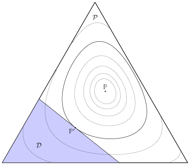
Figure 1: Visualization of the LDP (7). If $\mathcal{D}\subseteq\mathcal{P}$ is $\rm I$-continuous and $\mathbb{P}\notin\mathcal{D}$, then the probability $\mathbb{P}^{\infty}(\hat{\mathbb{P}}_{T}\in\mathcal{D})$ decays at the exponential rate $\inf_{\mathbb{P}^{\prime}\in\mathcal{D}}\mathrm{I}(\mathbb{P}^{\prime},\mathbb{P})$, which can be viewed as the relative entropy distance of $\mathbb{P}$ from $\mathcal{D}$.

Theorem 3.5 (Strong LDP)

If the samples $\{\xi_{t}\}_{t\in\mathbb{N}}$ are drawn independently from some $\mathbb{P}\in\mathcal{P}$, then for every Borel set $\mathcal{D}\subseteq\mathcal{P}$ the sequence of empirical distributions $\{\hat{\mathbb{P}}_{T}\}_{T\in\mathcal{P}}$ satisfies

$$\mathbb{P}^{\infty}\left(\hat{\mathbb{P}}_{T}\in\mathcal{D}\right) \leq(T+1)^{d}e^{-T\inf_{\mathbb{P}^{\prime}\in\mathcal{D}}\,\mathrm{I}(\mathbb{P}^{\prime},\mathbb{P})}\quad\forall T\in\mathbb{N}.$$ (9)

Proof 3.6

Proof. The claim follows immediately from inequality (6.1) in the proof of Theorem 3.4 in Appendix 6. Note that (6.1) does not rely on the assumption that $\mathbb{P}>0$. $\square$

4 Distributionally robust predictors and prescriptors are optimal

Armed with the fundamental results of large deviations theory, we now endeavor to identify the least conservative data-driven predictors and prescriptors whose out-of-sample disappointment decays at a rate no less than some prescribed threshold $r>0$ under any model $\mathbb{P}\in\mathcal{P}$, that is, we aim to solve the vector optimization problems (5) and (6).

4.1 Distributionally robust predictors

The relative entropy lends itself to constructing a data-driven predictor in the sense of Definition 2.3. We will show below that this predictor is strongly optimal in (5).

Definition 4.1 (Distributionally robust predictors)

For any fixed threshold $r\geq 0$, we define the data-driven predictor $\hat{c}_{r}:X\times\mathcal{P}\to\Re$ through

$$\hat{c}_{r}(x,\mathbb{P}^{\prime})=\sup_{\mathbb{P}\in\mathcal{P}}\,\left\{c(x,\mathbb{P}):\mathrm{I}(\mathbb{P}^{\prime},\mathbb{P})\leq r\right\}\qquad\forall x\in X,~{}\mathbb{P}^{\prime}\in\mathcal{P}.$$ (10)

The data-driven predictor $\hat{c}_{r}$ admits a distributionally robust interpretation. In fact, $\hat{c}_{r}(x,\mathbb{P}^{\prime})$ represents the worst-case expected cost associated with the decision $x$, where the worst case is taken across all models $\mathbb{P}\in\mathcal{P}$ whose relative entropy distance to $\mathbb{P}^{\prime}$ is at most $r$. Observe that the supremum in (10) is always attained because $c(x,\mathbb{P})$ is linear in $\mathbb{P}$ and the feasible set of (10) is compact, which follows from the compactness of $\mathcal{P}$ and the lower semicontinuity of the relative entropy in $\mathbb{P}$ for any fixed $\mathbb{P}^{\prime}$; see Proposition 3.2(iii). Note also that $\hat{c}_{r}(x,\mathbb{P}^{\prime})$ can be evaluated efficiently because (10) constitutes a convex conic optimization problem with $d$ decision variables. A particularly simple and efficient method to evaluate $\hat{c}_{r}(x,\mathbb{P}^{\prime})$ is to solve the one-dimensional convex minimization problem dual to (10) by using bisection or another line search method.

Proposition 4.2 (Dual representation of $\hat{c}_{r}$)

If $r>0$ and $\bar{\gamma}(x)=\max_{i\in\Xi}\,\gamma(x,i)$ denotes the worst-case cost function, then the distributionally robust predictor admits the dual representation

$$\hat{c}_{r}(x,\mathbb{P}^{\prime})=\min_{\alpha\geq\bar{\gamma}(x)}\alpha-e^{-r}\prod_{i\in\Xi}\left(\alpha-\gamma(x,i)\right)^{\mathbb{P}^{\prime}(i)}.$$ (11)

Problem (11) has a minimizer $\alpha^{\star}$ that satisfies $\bar{\gamma}(x)\leq\alpha^{\star}\leq\frac{\bar{\gamma}(x)-e^{-r}c(x,\mathbb{P}^{\prime})}{1-e^{-r}}$.

Proof 4.3

Proof. See Appendix 6. $\square$

Remark 4.4 (Sample average predictor)

For $r=0$ the distributionally robust predictor $\hat{c}_{r}$ collapses to the sample average predictor of Example 2.4. Indeed, because of the strict positivity of the relative entropy $\mathrm{I}(\mathbb{P}^{\prime},\mathbb{P})>0$ for $\mathbb{P}^{\prime}\neq\mathbb{P}$, see Proposition 3.2(i), we have that

$$\hat{c}_{0}(x,\mathbb{P}^{\prime})=c(x,\mathbb{P}^{\prime}).$$

As shown in Example 2.6, the sample average predictor fails to offer asymptotic or finite sample guarantees of the form (3) and (4), respectively.

Remark 4.5 (Alternative distributionally robust predictors)

The relative entropy can also be used to construct a reverse distributionally robust predictor $\check{c}_{r}\in\mathcal{C}$ defined through

$$\check{c}_{r}(x,\mathbb{P}^{\prime})=\sup_{\mathbb{P}\in\mathcal{P}}\,\left\{c(x,\mathbb{P}):\mathrm{I}(\mathbb{P},\mathbb{P}^{\prime})\leq r\right\}\qquad\forall x\in X,~{}\mathbb{P}^{\prime}\in\mathcal{P}.$$ (12)

In contrast to $\hat{c}_{r}$, the reverse distributionally robust predictor $\check{c}_{r}$ fixes the second argument of the relative entropy and maximizes over the first argument. Note that $\check{c}_{r}$ can be viewed as the entropic value-at-risk of the uncertain cost $\gamma(x,\xi)$; see (Ahmadi-Javid 2012, Theorem 3.3). Another predictor related to $\hat{c}$ is the restricted distributionally robust predictor $\bar{c}_{r}\in\mathcal{C}$ defined through

$$\bar{c}_{r}(x,\mathbb{P}^{\prime})=\sup_{\mathbb{P}\in\mathcal{P}}\,\left\{c(x,\mathbb{P}):\mathbb{P}\ll\mathbb{P}^{\prime},~{}\mathrm{I}(\mathbb{P}^{\prime},\mathbb{P})\leq r\right\}\qquad\forall x\in X,~{}\mathbb{P}^{\prime}\in\mathcal{P},$$ (13)

where $\mathbb{P}\ll\mathbb{P}^{\prime}$ expresses the requirement that $\mathbb{P}$ must be absolutely continuous with respect to $\mathbb{P}^{\prime}$. Formally, $\mathbb{P}\ll\mathbb{P}^{\prime}$ means that $\mathbb{P}(i)=0$ for all outcomes $i\in\Xi$ with $\mathbb{P}^{\prime}(i)=0$. By (Ahmadi-Javid 2012, Definition 5.1), $\bar{c}_{r}$ can be interpreted as the negative log-entropic risk of $\gamma(x,\xi)$.

The predictors $\hat{c}_{r}$ and $\check{c}_{r}$ differ because the relative entropy fails to be symmetric. We emphasize that the reverse predictor $\check{c}_{r}$ has appeared often in the literature on distributionally robust optimization, see, e.g., (Ben-Tal et al. 2013, Calafiore 2007, Hu and Hong 2013, Lam 2016b, Wang et al. 2016). The predictors $\hat{c}_{r}$ and $\bar{c}_{r}$ differ, too, because of the additional constraint $\mathbb{P}\ll\mathbb{P}^{\prime}$, which is significant when not all outcomes in $\Xi$ have been observed. The statistical properties of the predictor $\bar{c}_{r}$ have been analyzed by Lam (2016a) and more recently by Duchi et al. (2016) from the perspective of the empirical likelihood theory introduced by Owen (1988). The predictor $\hat{c}_{r}$ suggested here has not yet been studied extensively even though—as we will demonstrate below—it displays attractive theoretical properties that are not shared by either $\check{c}_{r}$ or $\bar{c}_{r}$. The difference between $\hat{c}_{r}$ and $\check{c}_{r}$ or $\bar{c}_{r}$ is significant. Indeed, both $\check{c}_{r}$ and $\bar{c}_{r}$ hedge only against models $\mathbb{P}$ that are absolutely continuous with respect to the (observed realization of the) empirical distribution $\mathbb{P}^{\prime}$. While it is clear that the empirical distribution must be absolutely continuous with respect to the data-generating distribution, however, the converse implication is generally false. Indeed, an outcome can have positive probability even if it does not show up in a given finite time series. By taking the worst case only over models that are absolutely continuous with respect to $\mathbb{P}^{\prime}$, both predictors $\check{c}_{r}$ and $\bar{c}_{r}$ potentially ignore many models that could have generated the observed data.

We first establish that $\hat{c}_{r}$ indeed belongs to the set $\mathcal{C}$ of all data-driven predictors, that is, the family of continuous functions mapping $X\times\mathcal{P}$ to the reals.

Proposition 4.6 (Continuity of $\hat{c}_{r}$)

If $r\geq 0$, then the distributionally robust predictor $\hat{c}_{r}$ is continuous on $X\times\mathcal{P}$.

Proof 4.7

Proof. By Proposition 4.2, the distributionally robust predictor $\hat{c}_{r}$ admits the dual representation (11). Note that the objective function of (11) is manifestly continuous in $(\alpha,x,\mathbb{P}^{\prime})$ and that (11) is guaranteed to have a minimizer in the compact interval $[\bar{\gamma}(x),\frac{\bar{\gamma}(x)-e^{-r}c(x,\mathbb{P}^{\prime})}{1-e^{-r}}]$, whose boundaries depend continuously on $(x,\mathbb{P}^{\prime})$. Consequently, the predictor $\hat{c}_{r}$ is continuous by Berge’s celebrated maximum theorem (Berge 1963, pp. 115–116). $\square$

We now analyze the performance of the distributionally robust data-driven predictor $\hat{c}_{r}$ using arguments from large deviations theory. The parameter $r$ encoding the predictor $\hat{c}_{r}$ captures the fundamental trade-off between out-of-sample disappointment and accuracy, which is inherent to any approach to data-driven prediction. Indeed, as $r$ increases, the predictor $\hat{c}_{r}$ becomes more reliable in the sense that its out-of-sample disappointment decreases. However, increasing $r$ also results in more conservative (pessimistically biased) predictions. In the following we will demonstrate that $\hat{c}_{r}$ strikes indeed an optimal balance between reliability and conservatism.

Theorem 4.8 (Feasibility of $\hat{c}_{r}$)

If $r\geq 0$, then the predictor $\hat{c}_{r}$ is feasible in (5).

Proof 4.9

Proof. From Proposition 4.6 we already know that $\hat{c}_{r}\in\mathcal{C}$. It remains to be shown that the out-of-sample disappointment of $\hat{c}_{r}$ decays at a rate of at least $r$. We have $c(x,\mathbb{P})>\hat{c}_{r}(x,\hat{\mathbb{P}}_{T})$ if and only if the estimator $\hat{\mathbb{P}}_{T}$ falls within the disappointment set

$$\mathcal{D}(x,\mathbb{P})=\left\{\mathbb{P}^{\prime}\in\mathcal{P}:c(x,\mathbb{P})>\hat{c}_{r}(x,\mathbb{P}^{\prime})\right\}.$$

Note that by the definition of $\hat{c}_{r}$, we have

$$\mathrm{I}(\mathbb{P}^{\prime},\mathbb{P})\leq r\quad\implies\quad\hat{c}_{r}(x,\mathbb{P}^{\prime})=\sup_{\mathbb{P}^{\prime\prime}\in\mathcal{P}}\left\{c(x,\mathbb{P}^{\prime\prime}):I(\mathbb{P}^{\prime},\mathbb{P}^{\prime\prime})\leq r\right\}\geq c(x,\mathbb{P}).$$

By contraposition, the above implication is equivalent to

$$c(x,\mathbb{P})>\hat{c}_{r}(x,\mathbb{P}^{\prime})\quad\implies\quad\mathrm{I}(\mathbb{P}^{\prime},\mathbb{P})>r.$$

Therefore, $\mathcal{D}(x,\mathbb{P})$ is a subset of

$$\mathcal{I}(\mathbb{P})=\left\{\mathbb{P}^{\prime}\in\mathcal{P}:\mathrm{I}(\mathbb{P}^{\prime},\mathbb{P})>r\right\}$$

irrespective of $x\in X$. We thus have

$$\limsup_{T\to\infty}\frac{1}{T}\log\mathbb{P}^{\infty}\left(\hat{\mathbb{P}}_{T}\in{\mathcal{D}}(x,\mathbb{P})\right)\leq\limsup_{T\to\infty}\frac{1}{T}\log\mathbb{P}^{\infty}\left(\hat{\mathbb{P}}_{T}\in\mathcal{I}(\mathbb{P})\right)\leq-\inf_{\mathbb{P}^{\prime}\in\mathcal{I}(\mathbb{P})}\,\mathrm{I}(\mathbb{P}^{\prime},\mathbb{P})\leq-r,$$

where the first inequality holds because ${\mathcal{D}}(x,\mathbb{P})\subseteq\mathcal{I}(\mathbb{P})$, while the second inequality exploits the weak LDP upper bound (7a). Thus, $\hat{c}_{r}$ is feasible in (5). $\square$

Note that any predictor $\hat{c}$ with $\hat{c}_{r}\preceq_{\mathcal{C}}\hat{c}$ has a smaller disappointment set than $\hat{c}_{r}$, and thus the out-of-sample disappointment of $\hat{c}$ decays at least as fast as that of $\hat{c}_{r}$. Hence, $\hat{c}$ is also feasible in (5). In particular, this immediately implies that if we inflate the relative entropy ball of the distributionally robust predictor $\hat{c}_{r}$ to any larger ambiguity set, we obtain another predictor that is feasible in (5). As an example, consider the total variation predictor

$$\hat{c}^{\rm{tv}}_{r}(x,\mathbb{P}^{\prime})=\sup_{\mathbb{P}\in\mathcal{P}}\,\left\{c(x,\mathbb{P}):\left\|\mathbb{P}-\mathbb{P}^{\prime}\right\|_{\rm{tv}}\leq\sqrt{2r}\right\}\qquad\forall x\in X,~{}\mathbb{P}^{\prime}\in\mathcal{P},$$

where $\left\|\mathbb{P}-\mathbb{P}^{\prime}\right\|_{\rm{tv}}$ denotes the total variation distance between $\mathbb{P}$ and $\mathbb{P}^{\prime}$. Pinsker’s classical inequality asserts that $\left\|\mathbb{P}-\mathbb{P}^{\prime}\right\|_{\rm{tv}}\leq\sqrt{2\,\mathrm{I}(\mathbb{P}^{\prime},\mathbb{P})}$ for all $\mathbb{P}$ and $\mathbb{P}^{\prime}$ in $\mathcal{P}$. Thus, we have $\hat{c}_{r}\preceq_{\mathcal{C}}\hat{c}^{\rm{tv}}_{r}$, which implies that the total variation predictor is feasible in (5). This suggests that (5) has a rich feasible set.

The following main theorem establishes that $\hat{c}_{r}$ is not only a feasible but even a strongly optimal solution for the vector optimization problem (5). This means that if an arbitrary data-driven predictor $\hat{c}$ predicts a lower expected cost than $\hat{c}_{r}$ even for a single estimator realization $\mathbb{P}^{\prime}\in\mathcal{P}$, then $\hat{c}$ must suffer from a higher out-of-sample disappointment than $\hat{c}_{r}$ to first order in the exponent.

Theorem 4.10 (Optimality of $\hat{c}_{r}$)

If $r>0$, then $\hat{c}_{r}$ is strongly optimal in (5).

Proof 4.11

Proof. Assume for the sake of argument that $\hat{c}_{r}$ fails to be a strong solution for (5). Thus, there exists a data-driven predictor $\hat{c}\in\mathcal{C}$ that is feasible in (5) but not dominated by $\hat{c}_{r}$, that is, $\hat{c}_{r}\npreceq_{\mathcal{C}}\hat{c}$. This means that there exists $x\in X$ and $\mathbb{P}^{\prime}_{0}\in\mathcal{P}$ with $\hat{c}_{r}(x,\mathbb{P}^{\prime}_{0})>\hat{c}(x,\mathbb{P}^{\prime}_{0})$. For later reference we set $\epsilon=\hat{c}_{r}(x,\mathbb{P}^{\prime}_{0})-\hat{c}(x,\mathbb{P}^{\prime}_{0})>0$. In the remainder of the proof we will demonstrate that $\hat{c}$ cannot be feasible in (5), which contradicts our initial assumption.

Let $\mathbb{P}_{0}\in\mathcal{P}$ be an optimal solution of problem (10) at $\mathbb{P}^{\prime}=\mathbb{P}^{\prime}_{0}$. Thus, we have $I(\mathbb{P}^{\prime}_{0},\mathbb{P}_{0})\leq r$ and

$$\hat{c}_{r}(x,\mathbb{P}^{\prime}_{0})=c(x,\mathbb{P}_{0}).$$ (14)

In the following we will first perturb $\mathbb{P}_{0}$ to obtain a model $\mathbb{P}_{1}$ that is $\frac{\epsilon}{2}$-suboptimal in (10) but satisfies $I(\mathbb{P}^{\prime}_{0},\mathbb{P}_{1})<r$. Subsequently, we will perturb $\mathbb{P}_{1}$ to obtain a model $\mathbb{P}_{2}$ that is $\epsilon$-suboptimal in (10) but satisfies $I(\mathbb{P}^{\prime}_{0},\mathbb{P}_{2})<r$ as well as $\mathbb{P}_{2}>0$.

To construct $\mathbb{P}_{1}$, consider all models $\mathbb{P}(\lambda)=\lambda\mathbb{P}^{\prime}_{0}+(1-\lambda)\mathbb{P}_{0}$, $\lambda\in[0,1]$, on the line segment between $\mathbb{P}^{\prime}_{0}$ and $\mathbb{P}_{0}$. As $r$ is strictly positive, the convexity of the relative entropy implies that

$$\mathrm{I}(\mathbb{P}_{0}^{\prime},\mathbb{P}(\lambda))\leq\lambda\mathrm{I}(\mathbb{P}_{0}^{\prime},\mathbb{P}_{0}^{\prime})+(1-\lambda)\mathrm{I}(\mathbb{P}_{0}^{\prime},\mathbb{P}_{0})\leq(1-\lambda)r<r\quad\forall\lambda\in(0,1].$$

Moreover, as the expected cost $c(x,\mathbb{P}(\lambda))$ changes continuously in $\lambda$, there exists a sufficiently small $\lambda_{1}\in(0,1]$ such that $\mathbb{P}_{1}=\mathbb{P}(\lambda_{1})$ and $r_{1}=\mathrm{I}(\mathbb{P}^{\prime}_{0},\mathbb{P}_{1})$ satisfy $0<r_{1}<r$ and

$$c(x,\mathbb{P}_{0})<c(x,\mathbb{P}_{1})+\frac{\epsilon}{2}.$$

To construct $\mathbb{P}_{2}$, we consider all models $\mathbb{P}(\lambda)=\lambda\mathbb{U}+(1-\lambda)\mathbb{P}_{1}$, $\lambda\in[0,1]$, on the line segment between the uniform distribution $\mathbb{U}$ on $\Xi$ and $\mathbb{P}_{1}$. By the convexity of the relative entropy we have

$$\mathrm{I}(\mathbb{P}_{0}^{\prime},\mathbb{P}(\lambda))\leq\lambda\mathrm{I}(\mathbb{P}_{0}^{\prime},\mathbb{U})+(1-\lambda)\mathrm{I}(\mathbb{P}_{0}^{\prime},\mathbb{P}_{1})\leq\lambda\mathrm{I}(\mathbb{P}_{0}^{\prime},\mathbb{U})+(1-\lambda)r_{1}\quad\forall\lambda\in[0,1].$$

As $r_{1}<r$ and the expected cost $c(x,\mathbb{P}(\lambda))$ changes continuously in $\lambda$, there exists a sufficiently small $\lambda_{2}\in(0,1]$ such that $\mathbb{P}_{2}=\mathbb{P}(\lambda_{2})$ and $r_{2}=\mathrm{I}(\mathbb{P}^{\prime}_{0},\mathbb{P}_{2})$ satisfy $0<r_{2}<r$, $\mathbb{P}_{2}>0$ and

$$c(x,\mathbb{P}_{0})<c(x,\mathbb{P}_{2})+\epsilon.$$ (15)

In summary, we thus have

$$\hat{c}(x,\mathbb{P}^{\prime}_{0})=\hat{c}_{r}(x,\mathbb{P}^{\prime}_{0})-\epsilon=c(x,\mathbb{P}_{0})-\epsilon<c(x,\mathbb{P}_{2})\leq\hat{c}_{r}(x,\mathbb{P}^{\prime}_{0}),$$ (16)

where the first equality follows from the definition of $\epsilon$, and the second equality exploits (14). Moreover, the strict inequality holds due to (15), and the weak inequality follows from the definition of $\hat{c}_{r}$ and the fact that $\mathrm{I}(\mathbb{P}^{\prime}_{0},\mathbb{P}_{2})=r_{2}<r$.

In the remainder of the proof we will argue that the prediction disappointment $\mathbb{P}_{2}^{\infty}(c(x,\mathbb{P}_{2})>\hat{c}(x,\hat{\mathbb{P}}_{T}))$ under model $\mathbb{P}_{2}$ decays at a rate of at most $r_{2}<r$ as the sample size $T$ tends to infinity. In analogy to the proof of Theorem 4.8, we define the set of disappointing estimator realizations as

$$\mathcal{D}(x,\mathbb{P}_{2})=\left\{\mathbb{P}^{\prime}\in\mathcal{P}\ :\ c(x,\mathbb{P}_{2})>\hat{c}(x,\mathbb{P}^{\prime})\right\}.$$

This set contains $\mathbb{P}^{\prime}_{0}$ due to the strict inequality in (16). Moreover, as $\hat{c}\in\mathcal{C}$ is continuous, $\mathcal{D}(x,\mathbb{P}_{2})$ is an open subset of $\mathcal{P}$. Thus, we find

$$\inf_{\mathbb{P}^{\prime}\in\operatorname{int}\mathcal{D}(x,\mathbb{P}_{2})}\,\mathrm{I}(\mathbb{P}^{\prime},\mathbb{P}_{2})=\inf_{\mathbb{P}^{\prime}\in\mathcal{D}(x,\mathbb{P}_{2})}\,\mathrm{I}(\mathbb{P}^{\prime},\mathbb{P}_{2})\leq\mathrm{I}(\mathbb{P}^{\prime}_{0},\mathbb{P}_{2})=r_{2},$$

where the inequality holds because $\mathbb{P}^{\prime}_{0}\in\mathcal{D}(x,\mathbb{P}_{0})$, and the last equality follows from the definition of $r_{2}$. As the empirical distributions $\{\hat{\mathbb{P}}_{T}\}_{T\in\mathbb{N}}$ obey the LDP lower bound (7b) under $\mathbb{P}_{2}>0$, we finally conclude that

$$-r<-r_{2}\leq-\inf_{\mathbb{P}^{\prime}\in\operatorname{int}\mathcal{D}(x,\mathbb{P}_{2})}\,\mathrm{I}(\mathbb{P}^{\prime},\mathbb{P}_{2})\leq\liminf_{T\rightarrow\infty}\frac{1}{T}\log\mathbb{P}_{2}^{\infty}\left(\hat{\mathbb{P}}_{T}\in\mathcal{D}(x,\mathbb{P}_{2})\right).$$

The above chain of inequalities implies, however, that $\hat{c}$ is infeasible in problem (5). This contradicts our initial assumption, and thus, $\hat{c}_{r}$ must indeed be a strong solution of (5). $\square$

Theorem 4.10 asserts that the distributionally robust predictor $\hat{c}_{r}$ is optimal among all data-driven predictors representable as continuous functions of the empirical distribution $\hat{\mathbb{P}}_{T}$. That is, any attempt to make it less conservative invariably increases the out-of-sample prediction disappointment. We remark that the class of predictors which depend on the data only through $\hat{\mathbb{P}}_{T}$ is vast. These predictors constitute arbitrary continuous functions of the data that are independent of the order in which the samples were observed. As the samples are independent and identically distributed, there are in fact no meaningful data-driven predictors that display a more general dependence on the data.

Note that in the above discussion all guarantees are fundamentally asymptotic in nature. Using Theorem 3.5 one can show, however, that $\hat{c}_{r}$ also satisfies finite sample guarantees.

Theorem 4.12 (Finite sample guarantee)

The out-of-sample disappointment of the distributionally robust predictor $\hat{c}_{r}$ enjoys the following finite sample guarantee under any model $\mathbb{P}\in\mathcal{P}$ and for any $x\in X$.

$$\mathbb{P}^{\infty}\left(c(x,\mathbb{P})>\hat{c}_{r}(x,\hat{\mathbb{P}}_{T})\right)\leq(T+1)^{d}e^{-rT}\quad\forall T\in\mathbb{N}$$ (17)

Proof 4.13

Proof. The proof of this result widely parallels that of Theorem 4.8 but uses the strong LDP upper bound (9) in lieu of the weak upper bound (7a). Details are omitted for brevity. $\square$

4.2 Distributionally robust prescriptors

The distributionally robust predictor $\hat{c}_{r}$ of Definition 4.1 induces a corresponding prescriptor.

Definition 4.14 (Distributionally robust prescriptors)

Denote by $\hat{c}_{r}$, $r\geq 0$, the distributionally robust data-driven predictor of Definition 4.1. We can then define the data-driven prescriptor $\hat{x}_{r}:\mathcal{P}\to X$ as a quasi-continuous function satisfying

$$\hat{x}_{r}(\mathbb{P}^{\prime})\in\arg\min_{x\in X}\,\hat{c}_{r}(x,\mathbb{P}^{\prime})\quad\forall\mathbb{P}^{\prime}\in\mathcal{P}.$$ (18)

Note that the minimum in (18) is attained because $X$ is compact and $\hat{c}_{r}$ is continuous due to Proposition 4.6. Thus, there exists at least one function $\hat{x}_{r}$ satisfying (18). In the next proposition we argue that this function can be chosen to be quasi-continuous as desired.

Proposition 4.15 (Quasi-continuity of $\hat{x}_{r}$)

If $r\geq 0$, then there exists a quasi-continuous data-driven predictor $\hat{x}_{r}$ satisfying (18).

Proof 4.16

Proof. Denote by $\Gamma(\mathbb{P}^{\prime})=\arg\min_{x\in X}\,\hat{c}_{r}(x,\mathbb{P}^{\prime})$ the argmin-mapping of problem (10), and observe that $\Gamma(\mathbb{P}^{\prime})$ is compact and non-empty for every $\mathbb{P}^{\prime}\in\mathcal{P}$ because $\hat{c}_{r}$ is continuous and $X$ is compact. As $X$ is independent of $\mathbb{P}^{\prime}$, Berge’s maximum theorem (Berge 1963, pp. 115–116) further implies that $\Gamma$ is upper semicontinuous. As $\mathcal{P}$ is a Baire space and $X$ is a metric space, (Matejdes 1987, Corollary 4) finally guarantees that there exists a quasi-continuous function $\hat{x}_{r}:\mathcal{P}\to X$ with $\hat{x}_{r}(\mathbb{P}^{\prime})\in\Gamma(\mathbb{P}^{\prime})$ for all $\mathbb{P}^{\prime}\in\mathcal{P}$. $\square$

Propositions 4.6 and 4.15 imply that $(\hat{c}_{r},\hat{x}_{r})$ belongs to the family $\mathcal{X}$ of all data-driven predictor-prescriptor-pairs. Using a similar reasoning as in Theorem 4.8, we now demonstrate that the out-of-sample disappointment of $\hat{x}_{r}$ decays at rate at least $r$ as $T$ tends to infinity. Thus, $\hat{x}_{r}$ provides trustworthy prescriptions.

Theorem 4.17 (Feasibility of $(\hat{c}_{r},\hat{x}_{r})$)

If $r\geq 0$, then the predictor-prescriptor-pair $(\hat{c}_{r},\hat{x}_{r})$ is feasible in (6).

Proof 4.18

Proof. Propositions 4.6 and 4.15 imply that $(\hat{c}_{r},\hat{x}_{r})\in\mathcal{X}$. It remains to be shown that the out-of-sample disappointment of $\hat{x}_{r}$ decays at a rate of at least $r$. To this end, define $\mathcal{D}(x,\mathbb{P})$ and $\mathcal{I}(\mathbb{P})$ as in the proof of Theorem 4.8, and recall that $\mathcal{D}(x,\mathbb{P})\subseteq\mathcal{I}(\mathbb{P})$ for every decision $x\in X$ and model $\mathbb{P}\in\mathcal{P}$. Thus, for every fixed estimator realization $\mathbb{P}^{\prime}\in\mathcal{P}$ the following implication holds

$$c(\hat{x}_{r}(\mathbb{P}^{\prime}),\mathbb{P})>\hat{c}_{r}(\hat{x}_{r}(\mathbb{P}^{\prime}),\mathbb{P}^{\prime})\quad\implies\quad \exists x\in X\text{ with }c(x,\mathbb{P})>\hat{c}_{r}(x,\mathbb{P}^{\prime})$$

$$\implies\quad \mathbb{P}^{\prime}\in\cup_{x\in X}\mathcal{D}(x,\mathbb{P})$$

$$\implies\quad \mathbb{P}^{\prime}\in\mathcal{I}(\mathbb{P}),$$

which in turn implies

$$\limsup_{T\to\infty}\frac{1}{T}\log\mathbb{P}^{\infty}\left(c(\hat{x}_{r}(\hat{\mathbb{P}}_{T}),\mathbb{P})>\hat{c}_{r}(\hat{x}_{r}(\hat{\mathbb{P}}_{T}),\hat{\mathbb{P}}_{T})\right)\leq\limsup_{T\to\infty}\frac{1}{T}\log\mathbb{P}^{\infty}\left(\hat{\mathbb{P}}_{T}\in\mathcal{I}(\mathbb{P})\right)\leq-r$$

for every model $\mathbb{P}\in\mathcal{P}$. Note that the second inequality in the above expression has already been established in the proof of Theorem 4.8. Thus, the claim follows. $\square$

Next, we argue that $(\hat{c}_{r},\hat{x}_{r})$ is a strongly optimal solution for the vector optimization problem (6).

Theorem 4.19 (Optimality of $(\hat{c}_{r},\hat{x}_{r})$)

If $r>0$, then $(\hat{c}_{r},\hat{x}_{r})$ is strongly optimal in (6).

Proof 4.20

Proof. Assume for the sake of argument that $(\hat{c}_{r},\hat{x}_{r})$ fails to be a strong solution for (6). Thus, there exists a data-driven prescriptor $(\hat{c},\hat{x})\in\mathcal{X}$ that is feasible in (6) but not dominated by $(\hat{c}_{r},\hat{x}_{r})$, that is, $(\hat{c}_{r},\hat{x}_{r})\npreceq_{\mathcal{X}}(\hat{c},\hat{x})$. This means that there exists $\mathbb{P}_{0}^{\prime}\in\mathcal{P}$ with $\hat{c}_{r}(\hat{x}_{r}(\mathbb{P}^{\prime}_{0}),\mathbb{P}^{\prime}_{0})>\hat{c}(\hat{x}(\mathbb{P}^{\prime}_{0}),\mathbb{P}^{\prime}_{0})$. As $X$ is compact and $\hat{c}$ is continuous, the cost $\hat{c}(\hat{x}(\mathbb{P}^{\prime}),\mathbb{P}^{\prime})$ of the prescriptor $\hat{x}$ under the corresponding predictor $\hat{c}$ is continuous in $\mathbb{P}^{\prime}$ (Berge 1963, pp. 115–116). Similarly, $\hat{c}_{r}(\hat{x}_{r}(\mathbb{P}^{\prime}),\mathbb{P}^{\prime})$ is continuous in $\mathbb{P}^{\prime}$. Recall also that $\hat{x}$ is quasi-continuous and therefore continuous on a dense subset of $\mathcal{P}$ (Bledsoe 1952). Thus, we may assume without loss of generality that $\hat{x}$ is continuous at $\mathbb{P}_{0}^{\prime}$. For later reference we set $\epsilon=\hat{c}_{r}(\hat{x}(\mathbb{P}^{\prime}_{0}),\mathbb{P}^{\prime}_{0})-\hat{c}(\hat{x}(\mathbb{P}^{\prime}_{0}),\mathbb{P}^{\prime}_{0})>0$.

In the remainder of the proof we will demonstrate that $(\hat{c},\hat{x})$ cannot be feasible in (6), which contradicts our initial assumption. To this end, let $\mathbb{P}_{0}\in\mathcal{P}$ be an optimal solution of problem (10) at $x=\hat{x}(\mathbb{P}^{\prime}_{0})$ and $\mathbb{P}^{\prime}=\mathbb{P}^{\prime}_{0}$. Thus, we have $I(\mathbb{P}^{\prime}_{0},\mathbb{P}_{0})\leq r$ and

$$\hat{c}_{r}(\hat{x}(\mathbb{P}^{\prime}_{0}),\mathbb{P}^{\prime}_{0})=c(\hat{x}(\mathbb{P}^{\prime}_{0}),\mathbb{P}_{0}).$$ (19)

Next, we first perturb $\mathbb{P}_{0}$ to obtain a model $\mathbb{P}_{1}$ that is strictly $\frac{\epsilon}{2}$-suboptimal in (10) but satisfies $I(\mathbb{P}^{\prime}_{0},\mathbb{P}_{1})=r_{1}<r$. Subsequently, we perturb $\mathbb{P}_{1}$ to obtain a model $\mathbb{P}_{2}$ that is strictly $\epsilon$-suboptimal in (10) but satisfies $I(\mathbb{P}^{\prime}_{0},\mathbb{P}_{2})=r_{2}<r$ as well and $\mathbb{P}_{2}>0$. The distributions $\mathbb{P}_{1}$ and $\mathbb{P}_{2}$ can be constructed exactly as in the proof of Theorem 4.10. Details are omitted for brevity. Thus, we find

$$\hat{c}(\hat{x}(\mathbb{P}^{\prime}_{0}),\mathbb{P}^{\prime}_{0})=\hat{c}_{r}(\hat{x}(\mathbb{P}^{\prime}_{0}),\mathbb{P}^{\prime}_{0})-\epsilon=c(\hat{x}(\mathbb{P}^{\prime}_{0}),\mathbb{P}_{0})-\epsilon<c(\hat{x}(\mathbb{P}^{\prime}_{0}),\mathbb{P}_{2})\leq\hat{c}_{r}(\hat{x}(\mathbb{P}^{\prime}_{0}),\mathbb{P}^{\prime}_{0}),$$ (20)

where the first equality follows from the definition of $\epsilon$, and the second equality exploits (19). Moreover, the strict inequality holds because $\mathbb{P}_{2}$ is strictly $\epsilon$-suboptimal in (10), while the weak inequality follows from the definition of $\hat{c}_{r}$ and the fact that $I(\mathbb{P}^{\prime}_{0},\mathbb{P}_{2})=r_{2}<r$.

It remains to be shown that the prediction disappointment $\mathbb{P}_{2}^{\infty}(c(\hat{x}(\hat{\mathbb{P}}_{T}),\mathbb{P}_{2})>\hat{c}(\hat{x}(\hat{\mathbb{P}}_{T}),\hat{\mathbb{P}}_{T}))$ under model $\mathbb{P}_{2}$ decays at a rate of at most $r_{2}<r$ as the sample size $T$ tends to infinity. To this end, we define the set of disappointing estimator realizations as

$$\mathcal{D}(\mathbb{P}_{2})=\left\{\mathbb{P}^{\prime}\in\mathcal{P}\ :\ c(\hat{x}(\mathbb{P}^{\prime}),\mathbb{P}_{2})>\hat{c}(\hat{x}(\mathbb{P}^{\prime}),\mathbb{P}^{\prime})\right\}.$$

This set contains $\mathbb{P}^{\prime}_{0}$ due to the strict inequality in (20). Recall now that $\hat{x}$ is continuous at $\mathbb{P}^{\prime}=\mathbb{P}^{\prime}_{0}$ due to our choice of $\mathbb{P}^{\prime}_{0}$. As the predictors $\hat{c}$ and $\hat{c}_{r}$ are both continuous on their entire domain, the compositions $\hat{c}(\hat{x}(\mathbb{P}^{\prime}),\mathbb{P}^{\prime})$ and $c(\hat{x}(\mathbb{P}^{\prime}),\mathbb{P}_{2})$ are both continuous at $\mathbb{P}^{\prime}=\mathbb{P}^{\prime}_{0}$. This implies that $\mathbb{P}^{\prime}_{0}$ belongs actually to the interior of $\mathcal{D}(\mathbb{P}_{2})$. Thus, we find

$$\inf_{\mathbb{P}^{\prime}\in\operatorname{int}\mathcal{D}(\mathbb{P}_{2})}\,\mathrm{I}(\mathbb{P}^{\prime},\mathbb{P}_{2})\leq\mathrm{I}(\mathbb{P}^{\prime}_{0},\mathbb{P}_{2})=r_{2},$$

where the last equality follows from the definition of $r_{2}$. As the empirical distributions $\{\hat{\mathbb{P}}_{T}\}_{T\in\mathbb{N}}$ obey the LDP lower bound (7b) under $\mathbb{P}_{2}>0$, we finally conclude that

$$-r<-r_{2}\leq-\inf_{\mathbb{P}^{\prime}\in\operatorname{int}\mathcal{D}(\mathbb{P}_{2})}\,\mathrm{I}(\mathbb{P}^{\prime},\mathbb{P}_{2})\leq\liminf_{T\rightarrow\infty}\frac{1}{T}\log\mathbb{P}_{2}^{\infty}\left(\hat{\mathbb{P}}_{T}\in\mathcal{D}(\mathbb{P}_{2})\right).$$

The above chain of inequalities implies, however, that $(\hat{c},\hat{x})$ is infeasible in problem (6). This contradicts our initial assumption, and thus, $(\hat{c}_{r},\hat{x}_{r})$ must indeed be a strong solution of (6). $\square$

All guarantees discussed so far are asymptotic in nature. As in the case of the predictor $\hat{c}_{r}$, however, the prescriptor $\hat{x}_{r}$ can also be shown to satisfy finite sample guarantees.

Theorem 4.21 (Finite sample guarantee)

The out-of-sample disappointment of the distributionally robust prescriptor $\hat{x}_{r}$ enjoys the following finite sample guarantee under any model $\mathbb{P}\in\mathcal{P}$.

$$\mathbb{P}^{\infty}\left(c(\hat{x}_{r}(\hat{\mathbb{P}}_{T}),\mathbb{P})>\hat{c}_{r}(\hat{x}_{r}(\hat{\mathbb{P}}_{T}),\hat{\mathbb{P}}_{T})\right)\leq(T+1)^{d}e^{-rT}\quad\forall T\in\mathbb{N}$$ (21)

Proof 4.22

Proof. The proof of this result parallels those of Theorems 4.8 and 4.17 but uses the strong LDP upper bound (9) in lieu of the weak upper bound (7a). Details are omitted for brevity. $\square$

We stress that the finite sample guarantees of Theorems 4.12 and 4.21 as well as the strong optimality properties portrayed in Theorems 4.10 and 4.19 are independent of a particular dataset. They guarantee that $\hat{c}_{r}$ and $\hat{x}_{r}$ provide trustworthy predictions and prescriptions, respectively, before the data is revealed.

Remark 4.23 (Optimal hypothesis testing)

Bertsimas et al. (2018b) propose to construct predictors and prescriptors from statistical hypothesis tests. A hypothesis test uses i.i.d. samples $\xi_{1},\dots,\xi_{T}$ drawn from the unknown true distribution $\mathbb{P}^{\star}$ to decide whether the null hypothesis $\mathbb{P}^{\star}=\mathbb{P}$ is false for a fixed model $\mathbb{P}\in\mathcal{P}$. Specifically, the null hypothesis is rejected (it is declared that $\mathbb{P}^{\star}\neq\mathbb{P}$) if the empirical distribution $\hat{\mathbb{P}}_{T}$ associated with the observed sample path falls outside of a (measurable) acceptance region $A_{T}(\mathbb{P})\subseteq\mathcal{P}$, which depends on the conjectured model $\mathbb{P}$ and the sample size $T$. Otherwise, it is deemed that there is insufficient data to reject the null hypothesis.

Bertsimas et al. (2018b) associate with each hypothesis test a predictor

$$\hat{c}(x,\mathbb{P}^{\prime})=\left\{\begin{array}[]{r@{\hspace{0.75em}}l}\sup\hskip 7.5pt&c(x,\mathbb{P})\\[5.0pt] \mathrm{s.t.}\hskip 7.5pt&\mathbb{P}\in\mathcal{P}\\[5.0pt] \hskip 7.5pt&\mathbb{P}^{\prime}\in A_{T}(\mathbb{P}),\end{array}\right.$$ (22)

which evaluates the worst-case expected cost across all models $\mathbb{P}\in\mathcal{P}$ that pass the hypothesis test in view of the realization $\mathbb{P}^{\prime}\in\mathcal{P}_{T}=\mathcal{P}\cap\{0,1/T,\dots,(T-1)/T,1\}^{d}$ of the empirical distribution $\hat{\mathbb{P}}_{T}$.

The quality of a hypothesis test is usually measured by its type I error $\mathbb{P}^{\infty}(\hat{\mathbb{P}}_{T}\not\in A_{T}(\mathbb{P}))$, that is, the probability of falsely rejecting the null hypothesis, as well as its type II error $\mathbb{Q}^{\infty}(\hat{\mathbb{P}}_{T}\in A_{T}(\mathbb{P}))$, that is, the probability of falsely accepting the null hypothesis if the data follows a distribution $\mathbb{Q}\neq\mathbb{P}$. A particularly popular test is the likelihood ratio test, which uses the acceptance region

$$A^{\star}_{T}(\mathbb{P})=\left\{\mathbb{P}^{\prime}\in\mathcal{P}_{T}\ :\ \textstyle{\mathbb{P}^{\infty}(\hat{\mathbb{P}}_{T}=\mathbb{P}^{\prime})}/{\sup_{\mathbb{Q}\neq\mathbb{P}}\mathbb{Q}^{\infty}(\hat{\mathbb{P}}_{T}=\mathbb{P}^{\prime})}\geq e^{-rT}\right\}.$$

Zeitouni et al. (1992) prove that the likelihood ratio test is optimal in the following sense. Among all hypothesis tests whose type I error decays at a rate of at least $r$, $\limsup_{T\to\infty}\frac{1}{T}\log\mathbb{P}^{\infty}(\hat{\mathbb{P}}_{T}\notin A_{T}(\mathbb{P}))\leq-r$, the likelihood ratio test minimizes the nagative decay rate of the type II error $\limsup_{T\to\infty}\frac{1}{T}\log\mathbb{Q}^{\infty}(\hat{\mathbb{P}}_{T}\in A_{T}(\mathbb{P}))$ simultaneously for all models $\mathbb{Q}\in\mathcal{P}$ with $\mathbb{Q}\neq\mathbb{P}$. Cover and Thomas (2006, Theorem 11.1.2) further establish that the likelihood ratio of an estimator realization $\mathbb{P}^{\prime}\in\mathcal{P}_{T}$ under two alternative distributions $\mathbb{Q}$ and $\mathbb{P}$ satisfies $\log({\mathbb{P}^{\infty}(\hat{\mathbb{P}}_{T}=\mathbb{P}^{\prime})}/{\mathbb{Q}^{\infty}(\hat{\mathbb{P}}_{T}=\mathbb{P}^{\prime})})=-T(\mathrm{I}(\mathbb{P}^{\prime},\mathbb{P})-\mathrm{I}(\mathbb{P}^{\prime},\mathbb{Q}))$. The acceptance region of the likelihood ratio test thus simplifies to

$$A_{T}^{\star}(\mathbb{P})=\left\{\mathbb{P}^{\prime}\in\mathcal{P}_{T}\ :\ \textstyle\mathrm{I}(\mathbb{P}^{\prime},\mathbb{P})\leq r+\inf_{\mathbb{Q}\neq\mathbb{P}}\mathrm{I}(\mathbb{P}^{\prime},\mathbb{Q})\right\}=\left\{\mathbb{P}^{\prime}\in\mathcal{P}_{T}\ :\ \mathrm{I}(\mathbb{P}^{\prime},\mathbb{P})\leq r\right\},$$

where the equality holds because $\inf_{\mathbb{Q}\neq\mathbb{P}}\mathrm{I}(\mathbb{P}^{\prime},\mathbb{Q})=0$. Hence, the distributionally robust predictor $\hat{c}_{r}$ that is strongly optimal in the meta-optimization problem (5) coincides with the hypothesis test-based predictor (22) corresponding to the likelihood ratio test.

5 Extension to continuous state spaces

Assume now that the realizations of the random parameter $\xi$ may range over an arbitrary compact set $\Xi\subseteq\Re^{d}$ that is not necessarily finite. In analogy to the discrete case, we denote by $\mathcal{P}$ the family of all Borel probability distributions supported on $\Xi$. Note that $\mathcal{P}$ is now a convex subset of an infinite-dimensional space, which significantly complicates the problem of finding optimal predictors and prescriptors. We equip $\mathcal{P}$ with the standard topology of weak convergence of distributions, recalling that the weak topology is metrized by the Prokhorov metric (Prokhorov 1956). Consequently, we equip $X\times\mathcal{P}$ with the product of the standard Euclidean topology on $X$ and the weak topology on $\mathcal{P}$. In the remainder of this section we analyze to what extent—and under what additional conditions—the results for finite state spaces carry over to the more general continuous case. As this analysis requires more subtle mathematical techniques, we relegate all proofs to Appendix 6.

We first note that the definitions of model-based predictors and prescriptors require no changes. In order to evaluate the expectation in the definition of the model-based predictor $c(x,\mathbb{P})=\int_{\Xi}\gamma(x,\xi)\mathrm{d}\mathbb{P}(\xi)$, however, we now need to evaluate an integral with respect to $\mathbb{P}$ instead of a finite sum. Throughout this section we assume that the cost function $\gamma(x,\xi)$ is jointly continuous in $x$ and $\xi$. This implies via the compactness of $X$ and $\Xi$ that $c(x,\mathbb{P})$ is continuous in $x$ and $\mathbb{P}$, which in turn guarantees that a model-based prescriptor $x^{\star}(\mathbb{P})\in\arg\min_{x\in X}c(x,\mathbb{P})$ exists for every $\mathbb{P}\in\mathcal{P}$.

Lemma 5.1 (Continuity of model-based predictors)

If $\gamma(x,\xi)$ is continuous on the compact set $X\times\Xi$, then $c(x,\mathbb{P})$ is continuous on $X\times\mathcal{P}$.

As in the case of a discrete state space, we study data-driven predictors and prescriptors that depend on the training data $\{\xi_{t}\}_{t=1}^{T}$ only through the empirical distribution. Because $\Xi$ may now have infinite cardinality, we redefine the empirical distribution as $\hat{\mathbb{P}}_{T}=\frac{1}{T}\sum_{t=1}^{T}\delta_{\xi_{t}}$, where $\delta_{\xi_{t}}$ denotes the Dirac point mass at $\xi_{t}$. Using this new definition of $\hat{\mathbb{P}}_{T}$, we then define data-driven predictors and prescriptors exactly as in Section 2.1. As $\Xi$ is compact, one can show that $\mathcal{P}$ is compact in the weak topology (Prokhorov 1956). Moreover, as the weak topology is metrized by the Prokhorov metric, $\mathcal{P}$ constitutes a (locally) compact metric space. The Baire category theorem thus implies that $\mathcal{P}$ is a Baire space (Baire 1899). Corollary 4 in (Matejdes 1987, p. 120), which applies because $\mathcal{P}$ is a Baire space and $X$ is a metric space, further ensures that for any valid (continuous) predictor $\hat{c}$ the set-valued mapping $\arg\min_{x\in X}\,\hat{c}(x,{\mathbb{P}^{\prime}})$ admits a quasi-continuous selector $\hat{x}$, which serves as a valid data-driven prescriptor. Using the exact same reasoning as in Section 2.1, one can show that the points of continuity of any quasi-continuous prescriptor are dense in $\mathcal{P}$.

The best predictors and predictor-prescriptor-pairs can again be found by solving the meta-optimization problems (5) and (6), respectively. In order to construct near-optimal solutions for these meta-optimization problems, we recall the definition of the relative entropy between arbitrary distributions $\mathbb{P}^{\prime}$ and $\mathbb{P}$ on a compact set $\Xi\subseteq\Re^{d}$.

Definition 5.2 (Generalized relative entropy)

The relative entropy of $\mathbb{P}^{\prime}\in\mathcal{P}$ with respect to $\mathbb{P}\in\mathcal{P}$ is defined as

$$\mathrm{I}(\mathbb{P}^{\prime},\mathbb{P})=\begin{cases}\int_{\Xi}\log\left({\mathrm{d}\mathbb{P}^{\prime}}/{\mathrm{d}\mathbb{P}}(\xi)\right)\mathrm{d}\mathbb{P}^{\prime}(\xi)&{\rm{if}~{}}\mathbb{P}^{\prime}\ll\mathbb{P},\\[5.0pt] +\infty&{\rm{otherwise,}}\end{cases}$$

where $\mathbb{P}^{\prime}\ll\mathbb{P}$ means that $\mathbb{P}^{\prime}$ is absolutely continuous with respect to $\mathbb{P}$, while ${\mathrm{d}\mathbb{P}^{\prime}}/{\mathrm{d}\mathbb{P}}(\xi)$ denotes the Radon-Nikodym derivative of $\mathbb{P}^{\prime}$ with respect to $\mathbb{P}$, which exists if $\mathbb{P}^{\prime}\ll\mathbb{P}$ (Nikodym 1930).

The properties of the relative entropy portrayed in Proposition 3.2 hold verbatim in the more general setting considered here (Van Erven and Harremoës 2014). Using the generalized definition of the relative entropy, the distributionally robust predictor $\hat{c}_{r}$ and the corresponding prescriptor $\hat{x}_{r}$ can be constructed as in Definitions 4.1 and 4.14, respectively. In the following we will show that the predictor $\hat{c}_{r}$ is continuous, which ensures that the prescriptor $\hat{x}_{r}$ can always be chosen to be quasi-continuous. To this end, we first derive a dual representation for $\hat{c}_{r}$.

Proposition 5.3 (Dual representation revisited)

If $r>0$ and $\bar{\gamma}(x)=\max_{\xi\in\Xi}\,\gamma(x,\xi)$ is the worst-case cost function, then the distributionally robust predictor admits the dual representation

$$\hat{c}_{r}(x,\mathbb{P}^{\prime})=\min_{\alpha\geq\bar{\gamma}(x)}\alpha-e^{-r}\cdot\exp\left(\int_{\Xi}\log\left(\alpha-\gamma(x,\xi)\right)\mathrm{d}\mathbb{P}^{\prime}(\xi)\right).$$ (23)

Problem (23) has a minimizer $\alpha^{\star}\leq\frac{\bar{\gamma}(x)-e^{-r}c(x,\mathbb{P}^{\prime})}{1-e^{-r}}$.

Proposition 5.3 extends Proposition 4.2 to compact continuous state spaces and suggests that $\hat{c}_{r}(x,\mathbb{P}^{\prime})$ can be computed via bisection or other line search methods. Thus, the computational tractability of problem (23) largely hinges on our ability to efficiently evaluate the geometric mean $\exp\left(\int_{\Xi}\log\left(\alpha-\gamma(x,\xi)\right)\mathrm{d}\mathbb{P}^{\prime}(\xi)\right)$ for any fixed $\alpha$. For example, if $\mathbb{P}^{\prime}$ coincides with (a realization of) the empirical distribution $\hat{\mathbb{P}}_{T}$, we recover the geometric mean of $\alpha-\gamma(x,\xi)$ along a sample path, which can be reformulated as the optimal value of a tractable second-order cone program involving $\mathcal{O}(T)$ constraints and auxiliary variables (Nesterov and Nemirovskii 1994, Section 6.2.3.5).

$$\exp\left(\int_{\Xi}\log\left(\alpha-\gamma(x,\xi)\right)\mathrm{d}\mathbb{P}^{\prime}(\xi)\right)=\left(\prod_{t=1}^{T}\left(\alpha-\gamma(x,\xi_{t})\right)\right)^{1/T}$$

To our best knowledge, the dual representation (23) is new. The closest result we are aware of is the dual representation of the negative log-entropic risk measure derived in (Ahmadi-Javid 2012, Theorem 5.1). Indeed, the negative log-entropic risk of $\gamma(x,\xi)$ coincides with the restricted distributionally robust predictor $\bar{c}_{r}(x,\mathbb{P}^{\prime})$. Recall from (13) that $\bar{c}_{r}(x,\mathbb{P}^{\prime})$ differs from $c_{r}(x,\mathbb{P}^{\prime})$ only in that it imposes the additional constraint $\mathbb{P}\ll\mathbb{P}^{\prime}$ when evaluating the worst-case expected cost. Using Theorem 5.1 by Ahmadi-Javid (2012) one can thus show that the dual representation of $\bar{c}_{r}(x,\mathbb{P}^{\prime})$ differs from (23) only in that it replaces $\bar{\gamma}(x)$ with $\inf\{\bar{\gamma}:\mathbb{P}^{\prime}[\gamma(x,\xi)\leq\bar{\gamma}]=1\}\leq\bar{\gamma}(x)$. Maybe surprisingly, however, the derivation of (23) provided here is substantially more challenging.

Proposition 5.4 (Continuity of $\hat{c}_{r}$ revisited)

If $r\geq 0$, then the distributionally robust predictor $\hat{c}_{r}$ is continuous on $X\times\mathcal{P}$.

Proposition 5.4 ensures that $\hat{c}_{r}\in\mathcal{C}$. As any continuous predictor induces a quasi-continuous prescriptor, we may thus conclude that there exists a valid distributionally robust prescriptor $\hat{x}_{r}$ such that $(\hat{c}_{r},\hat{x}_{r})\in\mathcal{X}$. It now only remains to establish that these predictors and predictor-prescriptor-pairs are the unique strong solutions of the meta-optimization problems (5) and (6), respectively. In Section 4 this was achieved by leveraging the weak LDP portrayed in Theorem 3.4. Luckily, this LDP carries over to the more general setting considered here—albeit with a subtle difference.

Theorem 5.5 (Weak LDP revisited)

If the samples $\{\xi_{t}\}_{t\in\mathbb{N}}$ are drawn independently from some $\mathbb{P}\in\mathcal{P}$, then for every set $\mathcal{D}\subseteq\mathcal{P}$ the sequence of empirical distributions $\{\hat{\mathbb{P}}_{T}\}_{T\in\mathbb{N}}$ satisfies

$$\limsup_{T\to\infty}~{}\frac{1}{T}\log\mathbb{P}^{\infty}(\hat{\mathbb{P}}_{T}\in\mathcal{D}) \leq-\inf_{\mathbb{P}^{\prime}\in\operatorname{cl}\mathcal{D}}\,\mathrm{I}(\mathbb{P}^{\prime},\mathbb{P}),$$ (24a)

$$\liminf_{T\to\infty}~{}\,\frac{1}{T}\log\mathbb{P}^{\infty}(\hat{\mathbb{P}}_{T}\in\mathcal{D}) \geq-\inf_{\mathbb{P}^{\prime}\in\operatorname{int}\mathcal{D}}\,\mathrm{I}(\mathbb{P}^{\prime},\mathbb{P}).$$ (24b)

Proof 5.6

Proof. See Csiszár (2006, Section 2). $\square$

Formally, Theorem 5.5 is almost identical to Theorem 3.4. However, the weak LDP upper bound (24a) differs from (7a) in that the minimization over all estimator realizations $\mathbb{P}^{\prime}$ on the right hand side runs over the closure of $\mathcal{D}$. This subtle difference invalidates the proof of Theorem 4.8, and thus we need a new approach to show that $\hat{c}_{r}$ is feasible in (5). Moreover, the weak LDP lower bound (24b) does not rely on any structural assumptions about $\mathbb{P}$. Note that the condition $\mathbb{P}>0$ in Theorem 3.4 was only imposed for convenience to simplify the proof of (7b) in Appendix 6.

As in the case of finite state spaces, one can now show that the distributionally robust predictor $\hat{c}_{r}$ is the unique strong solution of the meta-optimization problem (5).

Theorem 5.7 (Feasibility and optimality of $\hat{c}_{r}$ revisited)

If $r\geq 0$, then the predictor $\hat{c}_{r}$ is feasible in (5). Moreover, if $r>0$, then $\hat{c}_{r}$ is strongly optimal in (5).

While we did not manage to prove that $(\hat{c}_{r},\,\hat{x}_{r})$ is feasible in the meta-optimization problem (6), we still could show that it is essentially feasible and strongly optimal in a precise sense.

Theorem 5.8 (Feasibility and optimality of $(\hat{c}_{r},\hat{x}_{r})$ revisited)

If $r\geq 0$, then the shifted predictor-prescriptor-pair $(\hat{c}_{r}+\epsilon,\hat{x}_{r})$ is feasible in (6) for every $\epsilon>0$. Moreover, if $r>0$, then $(\hat{c}_{r},\hat{x}_{r})$ is preferred to every feasible solution of (6)—even though it may be infeasible.

Theorem 5.8 asserts that $(\hat{c}_{r},\hat{x}_{r})$ is less conservative than any predictor-prescriptor pair feasible in the meta-optimization problem (6) and that $(\hat{c}_{r},\hat{x}_{r})$ can be made feasible in (6) by shifting the distributionally robust predictor $\hat{c}_{r}$ up by just a tiny amount. For practical purposes this means that $(\hat{c}_{r},\hat{x}_{r})$ is indeed essentially optimal. Whether $(\hat{c}_{r},\,\hat{x}_{r})$ itself is feasible in (6) remains open.

We also emphasize that the strong LDP portrayed in Theorem 3.5 has no continuous counterpart, which implies that the finite sample guarantees of Theorems 4.12 and 4.21 cannot be generalized.

6 Proofs

Proof 6.1

Proof of Theorem 3.4. Let $i_{t}\in\Xi$ be a particular realization of the random variable $\xi_{t}$ for each $t=1,\ldots,T$, and denote by $\mathbb{P}^{\prime}$ the realization of the estimator $\hat{\mathbb{P}}_{T}$ corresponding to the sequence $\{i_{t}\}_{t=1}^{T}$. The probability of observing this sequence (in the given order) under model $\mathbb{P}$ can be expressed in terms of $\mathbb{P}^{\prime}$ as

$$\mathbb{P}^{\infty}(\xi_{1}=i_{1},\dots,\xi_{T}=i_{T})=\prod_{i\in\Xi}\mathbb{P}(i)^{T\mathbb{P}^{\prime}(i)}=e^{T\sum_{i\in\Xi}\mathbb{P}^{\prime}(i)\log\mathbb{P}(i)}.$$ (25)

Set $\mathcal{P}_{T}=\mathcal{P}\cap\{0,1/T,\dots,(T-1)/T,1\}^{d}$ and note that $\mathbb{P}^{\infty}(\hat{\mathbb{P}}_{T}\in\mathcal{P}_{T})=1$. By construction, the cardinality of $\mathcal{P}_{T}$ is bounded above by $(T+1)^{d}$.

In the following, we denote the set of all sample paths in $\Xi^{T}$ that give rise to the same empirical distribution $\mathbb{P}^{\prime}\in\mathcal{P}_{T}$ by $C_{T}(\mathbb{P}^{\prime})$. The cardinality of $C_{T}(\mathbb{P}^{\prime})$ coincides with the number of sample paths that visit state $i$ exactly $T\cdot\mathbb{P}^{\prime}(i)$ times for all $i\in\Xi$, that is, we have

$$\left|C_{T}(\mathbb{P}^{\prime})\right|=\frac{T!}{\prod_{i\in\Xi}(T\cdot\mathbb{P}^{\prime}(i))!}.$$

Stirling’s approximation for factorials allows us to bound the cardinality of $C_{T}(\mathbb{P}^{\prime})$ from both sides in terms of the entropy $H(\mathbb{P}^{\prime})=-\sum_{i=1}^{d}\mathbb{P}^{\prime}(i)\log\mathbb{P}^{\prime}(i)$ of the empirical distribution $\mathbb{P}^{\prime}$, that is,

$$(T+1)^{-d}e^{TH(\mathbb{P}^{\prime})}\leq\left|C_{T}(\mathbb{P}^{\prime})\right|\leq e^{TH(\mathbb{P}^{\prime})}.$$ (26)

An elementary proof of these inequalities that does not involve Stirling’s approximation is given by Cover and Thomas (2006, Theorem 12.1.3).

Select an arbitrary Borel set $\mathcal{D}\subseteq\mathcal{P}$. For any $T\in\mathbb{N}$, we thus have

$$\mathbb{P}^{\infty}(\hat{\mathbb{P}}_{T}\in\mathcal{D})= ~{}\sum_{\mathbb{P}^{\prime}\in\mathcal{D}\cap\mathcal{P}_{T}}\mathbb{P}^{\infty}(\hat{\mathbb{P}}_{T}=\mathbb{P}^{\prime})$$

$$\leq ~{}(T+1)^{d}\cdot\max_{\mathbb{P}^{\prime}\in\mathcal{D}\cap\mathcal{P}_{T}}\mathbb{P}^{\infty}(\hat{\mathbb{P}}_{T}=\mathbb{P}^{\prime})$$

$$\leq ~{}(T+1)^{d}\cdot\max_{\mathbb{P}^{\prime}\in\mathcal{D}\cap\mathcal{P}_{T}}\left|C_{T}(\mathbb{P}^{\prime})\right|e^{T\sum_{i\in\Xi}\mathbb{P}^{\prime}(i)\log\mathbb{P}(i)}$$

$$\leq ~{}(T+1)^{d}\cdot e^{-T\min_{\mathbb{P}^{\prime}\in\mathcal{D}\cap\mathcal{P}_{T}}\mathrm{I}(\mathbb{P}^{\prime},\mathbb{P})}$$

$$\leq ~{}(T+1)^{d}\cdot e^{-T\inf_{\mathbb{P}^{\prime}\in\mathcal{D}}\mathrm{I}(\mathbb{P}^{\prime},\mathbb{P})},$$

where the first inequality exploits the estimate $\left|\mathcal{P}_{T}\right|\leq(T+1)^{d}$, the second inequality holds due to (25) and the definition of $C_{T}(\mathbb{P}^{\prime})$, and the third inequality follows from the upper estimate in (26). Taking logarithms on both sides of the above expression and dividing by $T$ yields

$$\frac{1}{T}\log\mathbb{P}^{\infty}(\hat{\mathbb{P}}_{T}\in\mathcal{D})\leq ~{}\frac{d\log(T+1)}{T}-\inf_{\mathbb{P}^{\prime}\in\mathcal{D}}\mathrm{I}(\mathbb{P}^{\prime},\mathbb{P}).$$ (27)

Note that the finite sample bound (6.1) does not rely on any properties of the set $\mathcal{D}$ besides measurability. The asymptotic upper bound (7a) is obtained by taking the limit superior as $T$ tends to infinity on both sides of (6.1).

As for the lower bound (7b), recall that $\mathrm{I}(\mathbb{P}^{\prime},\mathbb{P})$ is continuous in $\mathbb{P}^{\prime}$ as $\mathbb{P}>0$, see Proposition 3.2(iii), and note that $\bigcup_{T\in\mathbb{N}}\mathcal{P}_{T}$ is dense in $\operatorname{int}\mathcal{D}$. Thus, there exists $T_{0}\in\mathbb{N}$ and a sequence of distributions $\mathbb{P}^{\prime}_{T}\in\mathcal{P}_{T}$, $T\in\mathbb{N}$, such that $\mathbb{P}^{\prime}_{T}\in\operatorname{int}\mathcal{D}$ for all $T\geq T_{0}$ and

$$\inf_{\mathbb{P}^{\prime}\in\operatorname{int}\mathcal{D}}\,\mathrm{I}(\mathbb{P}^{\prime},\mathbb{P})=\liminf_{T\rightarrow\infty}\,\mathrm{I}(\mathbb{P}^{\prime}_{T},\mathbb{P}).$$ (28)

Fix any $T\geq T_{0}$ and let $(i_{1},\ldots,i_{T})$ be a sequence of observations that generates $\mathbb{P}^{\prime}_{T}$. Then, we have

$$\mathbb{P}^{\infty}(\hat{\mathbb{P}}_{T}\in\mathcal{D})\geq ~{}\mathbb{P}^{\infty}(\hat{\mathbb{P}}_{T}=\mathbb{P}^{\prime}_{T})$$

$$= ~{}\left|C_{T}(\mathbb{P}^{\prime}_{T})\right|\cdot\mathbb{P}^{\infty}(\xi_{1}=i_{1},\dots,\xi_{T}=i_{T})$$

$$\geq ~{}(T+1)^{-d}\cdot e^{TH(\mathbb{P}^{\prime}_{T})}\cdot e^{T\sum_{i\in\Xi}\mathbb{P}^{\prime}_{T}(i)\log\mathbb{P}(i)}$$

$$= ~{}(T+1)^{-d}e^{-T\mathrm{I}(\mathbb{P}^{\prime}_{T},\mathbb{P})},$$

where the first inequality holds because $\mathbb{P}_{T}^{\prime}\in\operatorname{int}\mathcal{D}\subseteq\mathcal{D}$, while the second inequality follows from (25) and the lower estimate in (26). This implies that

$$\frac{1}{T}\log\mathbb{P}^{\infty}(\hat{\mathbb{P}}_{T}\in\mathcal{D})\geq-\frac{d\log(T+1)}{T}-\mathrm{I}(\mathbb{P}^{\prime}_{T},\mathbb{P})\quad\forall T\geq T_{0}.$$

Taking the limit inferior as $T$ tends to infinity on both sides of the above inequality and using (28) yields the postulated lower bound (7b). This completes the proof. $\square$

Proof 6.2

Proof of Proposition 4.2. Applying (Ben-Tal et al. 2013, Corollary 1) to the Burg entropy yields

$$\hat{c}_{r}(x,\mathbb{P}^{\prime})=\inf_{\alpha\geq\bar{\gamma}(x),\,\nu\geq 0}~{}\sum_{i\in\Xi}\nu\log\left(\frac{\nu}{\alpha-\gamma(x,i)}\right)\mathbb{P}^{\prime}(i)+\alpha+\nu(r-1)$$ (29)

for any $r>0$. In the following we denote the objective function of (29) by $g(\alpha,\nu)$, which is lower semicontinuous due to our conventions for the logarithm. As $g(\alpha,0)=\alpha$ and $\lim_{\nu\to\infty}g(\alpha,\nu)=\infty$, there must exist $\nu^{\star}(\alpha)\in\arg\min_{\nu\geq 0}g(\alpha,\nu)$ for any $\alpha\geq\bar{\gamma}(x)$. Indeed, if there is $i\in\Xi$ with $\alpha=\gamma(x,i)$ and $\mathbb{P}^{\prime}(i)>0$, then $\nu^{\star}(\alpha)=0$. Otherwise, $\nu^{\star}(\alpha)$ is the unique solution of the first-order optimality condition

$$\displaystyle\sum_{i\in\Xi}\left(\log\left(\frac{\nu^{\star}(\alpha)}{\alpha-\gamma(x,i)}\right)+1\right)\mathbb{P}^{\prime}(i)+r-1=0$$

$$\iff~{} \displaystyle\sum_{i\in\Xi}\log\left(\frac{\nu^{\star}(\alpha)}{\alpha-\gamma(x,i)}\right)\mathbb{P}^{\prime}(i)+r=0$$

$$\iff~{} \displaystyle\nu^{\star}(\alpha)=\exp\left(\sum_{i\in\Xi}\log\left(\alpha-\gamma(x,i)\right)\mathbb{P}^{\prime}(i)-r\right).$$

Thus, the partial minimum

$$g(\alpha,\nu^{\star}(\alpha))=\alpha-\exp\left(\sum_{i\in\Xi}\log\left(\alpha-\gamma(x,i)\right)\mathbb{P}^{\prime}(i)-r\right)=\alpha-e^{-r}\prod_{i\in\Xi}\left(\alpha-\gamma(x,i)\right)^{\mathbb{P}^{\prime}(i)}$$ (30)

is readily recognized as the objective function of problem (11), which is manifestly continuous in $\alpha$ and inherits convexity from $g(\alpha,\nu)$. By using Jensen’s inequality to interchange the logarithm and the expectation with respect to $\mathbb{P}^{\prime}$ in the second expression in (30), we find

$$g(\alpha,\nu^{\star}(\alpha))\geq\alpha-\sum_{i\in\Xi}\left(\alpha-\gamma(x,i)\right)\mathbb{P}^{\prime}(i)e^{-r}\geq\alpha(1-e^{-r})+e^{-r}\sum_{i\in\Xi}\gamma(x,i)\,\mathbb{P}^{\prime}(i).$$ (31)

As $r>0$, the above estimate implies that the partial minimum $g(\alpha,\nu^{\star}(\alpha))$ tends to infinity as $\alpha$ grows. Recalling that $\alpha$ is required to exceed $\bar{\gamma}(x)$, we may thus conclude that there exists $\alpha^{\star}$, such that $(\alpha^{\star},\nu^{\star}(\alpha^{\star}))$ attains the minimum in (11). Moreover, as $\alpha\geq\bar{\gamma}(x)\geq\gamma(x,i)$ for all $i\in\Xi$, we have $g(\alpha^{\star},\nu^{\star}(\alpha^{\star}))\leq\bar{\gamma}(x)$. Combining this upper bound with the lower bound (31) yields the estimate

$$\alpha^{\star}\leq\frac{\bar{\gamma}(x)}{1-e^{-r}}-\frac{e^{-r}}{1-e^{-r}}\sum_{i\in\Xi}\gamma(x,i)\,\mathbb{P}^{\prime}(i)=\frac{\bar{\gamma}(x)-e^{-r}c(x,\mathbb{P}^{\prime})}{1-e^{-r}}.$$

Thus, the claim follows. $\square$

Proof 6.3

Proof of Lemma 5.1. As the cost function $\gamma(x,\xi)$ is continuous and its domain $X\times\Xi$ is compact, the Heine-Cantor theorem implies that $\gamma(x,\xi)$ is uniformly continuous on its domain. Consider now an arbitrary converging sequence $(x_{i},\mathbb{P}_{i})$, $i\in\mathbb{N}$, in $X\times\mathcal{P}$, and denote its limit by $(x,\mathbb{P})$. The uniform continuity of the cost function ensures that for every $\delta>0$ there exists $N_{\delta}\in\mathbb{N}$ such that $\left|\gamma(x_{i},\xi)-\gamma(x,\xi)\right|\leq\delta$ uniformly across all $\xi\in\Xi$ and $i\geq N_{\delta}$, which in turn implies that

$$\left|\int_{\Xi}\gamma(x,\xi)\mathbb{P}(\mathrm{d}\xi)-\int_{\Xi}\gamma(x_{i},\xi)\mathrm{d}\mathbb{P}_{i}(\xi)\right|\leq\left|\int_{\Xi}\gamma(x,\xi)\mathrm{d}\mathbb{P}(\xi)-\int_{\Xi}\gamma(x,\xi)\mathrm{d}\mathbb{P}_{i}(\xi)\right|+\delta\quad\forall i\geq N_{\delta}.$$

As the integrant $\gamma(x,\xi)$ on the right hand side of the above inequality is continuous and bounded in $\xi$, and as the sequence $\mathbb{P}_{i}$, $i\in\mathbb{N}$, converges weakly to $\mathbb{P}$, we thus have $\lim_{i\to\infty}\left|\int_{\Xi}\gamma(x,\xi)\mathbb{P}(\mathrm{d}\xi)-\int_{\Xi}\gamma(x_{i},\xi)\mathbb{P}_{i}(\mathrm{d}\xi)\right|\leq\delta.$ As $\delta>0$ was chosen arbitrary, we may finally conclude that

$$\lim_{i\to\infty}\int_{\Xi}\gamma(x_{i},\xi)\mathbb{P}_{i}(\mathrm{d}\xi)=\int_{\Xi}\gamma(x,\xi)\mathbb{P}(\mathrm{d}\xi).$$

The claim then follows because the converging sequence $(x_{i},\mathbb{P}_{i})$, $i\in\mathbb{N}$, was chosen arbitrary. $\square$

In order to prove Proposition 5.3 we need three auxiliary lemmas. As a starting point, we first exploit the definition of the relative entropy between arbitrary distributions on a compact state space $\Xi$ to re-express the distributionally robust predictor explicitly as

$$\begin{array}[]{rcl}\hat{c}_{r}(x,\mathbb{P}^{\prime})=&\displaystyle\sup_{\mathbb{P}\in\mathcal{P}}&\displaystyle\int_{\Xi}\gamma(x,\xi)\,\mathrm{d}\mathbb{P}(\xi)\\[10.00002pt] &\mathrm{s.t.}&\mathbb{P}^{\prime}\ll\mathbb{P}\\[5.0pt] &&\displaystyle\int_{\Xi}\log\left(\frac{\mathrm{d}\mathbb{P}^{\prime}}{\mathrm{d}\mathbb{P}}(\xi)\right)\mathrm{d}\mathbb{P}^{\prime}(\xi)\leq r.\end{array}$$ (32)

Under the standing assumptions that $X$ and $\Xi$ are compact, while the cost function $\gamma(x,\xi)$ is jointly continuous in its arguments, the feasible set of problem (32) can be restricted to distributions $\mathbb{P}$ that are absolutely continuous with respect to $\mathbb{P}^{\prime}$ except perhaps on the compact set $\Xi^{\star}(x)=\arg\max_{\xi\in\Xi}\gamma(x,\xi)$.

Lemma 6.4 (Absolutely continuous representation of $\hat{c}_{r}$)

If $r\geq 0$ and $\bar{\gamma}(x)=\max_{\xi\in\Xi}\gamma(x,\xi)$ denotes the worst-case cost function, then the distributionally robust predictor $\hat{c}_{r}$ admits the equivalent representation

$$\begin{array}[]{rcl}\hat{c}_{r}(x,\mathbb{P}^{\prime})=&\displaystyle\sup_{\begin{subarray}{c}\mathbb{P}_{c}\in\mathcal{P}\\ p\in[0,1]\end{subarray}}&\displaystyle p\cdot\int_{\Xi}\gamma(x,\xi)\,\mathrm{d}\mathbb{P}_{c}(\xi)+(1-p)\cdot\bar{\gamma}(x)\\ &\mathrm{s.t.}&\mathbb{P}^{\prime}\ll p\cdot\mathbb{P}_{c}\ll\mathbb{P}^{\prime}\\[5.0pt] &&\displaystyle\int_{\Xi}\log\left(\frac{1}{p}\cdot\frac{\mathrm{d}\mathbb{P}^{\prime}}{\mathrm{d}\mathbb{P}_{c}}(\xi)\right)\mathrm{d}\mathbb{P}^{\prime}(\xi)\leq r.\end{array}$$ (33)

Proof 6.5

Proof. We first show that (32) provides an upper bound on (33). To this end, choose any $\mathbb{P}_{c}$ and $p$ feasible in (33), and define $\mathbb{P}=p\cdot\mathbb{P}_{c}+(1-p)\cdot\delta_{\xi^{\star}}\in\mathcal{P}$, where $\xi^{\star}\in\Xi^{\star}(x)$ represents an arbitrary worst-case scenario.

Note that $p>0$ for otherwise $\mathbb{P}^{\prime}\not\ll p\cdot\mathbb{P}_{c}$. The constraints of (33) and the construction of $\mathbb{P}$ thus imply that $\mathbb{P}^{\prime}\ll\mathbb{P}_{c}\ll\mathbb{P}$. By the Radon-Nikodym theorem (Nikodym 1930), we then have

$$\mathbb{P}^{\prime}[A] =\int_{A}\frac{\mathrm{d}\mathbb{P}^{\prime}}{\mathrm{d}\mathbb{P}}(\xi)\,\mathrm{d}\mathbb{P}(\xi)$$

and

$$\mathbb{P}^{\prime}[A] =\int_{A}\frac{\mathrm{d}\mathbb{P}^{\prime}}{\mathrm{d}\mathbb{P}_{c}}(\xi)\,\mathrm{d}\mathbb{P}_{c}(\xi)=\int_{A}\frac{1}{p}\cdot\frac{\mathrm{d}\mathbb{P}^{\prime}}{\mathrm{d}\mathbb{P}_{c}}(\xi)\cdot p\,\mathrm{d}\mathbb{P}_{c}(\xi)$$

$$=\int_{A}\frac{1}{p}\cdot\frac{\mathrm{d}\mathbb{P}^{\prime}}{\mathrm{d}\mathbb{P}_{c}}(\xi)\,\mathrm{d}\mathbb{P}(\xi)-\frac{1-p}{p}\cdot\frac{\mathrm{d}\mathbb{P}^{\prime}}{\mathrm{d}\mathbb{P}_{c}}(\xi^{\star})\leq\int_{A}\frac{1}{p}\cdot\frac{\mathrm{d}\mathbb{P}^{\prime}}{\mathrm{d}\mathbb{P}_{c}}(\xi)\,\mathrm{d}\mathbb{P}(\xi)$$

for all Borel sets $A\subseteq\Xi$, where the inequality in the last expression holds because Radon-Nikodym derivatives are pointwise non-negative. In summary, the above reasoning implies that

$$\frac{\mathrm{d}\mathbb{P}^{\prime}}{\mathrm{d}\mathbb{P}}(\xi)\leq\frac{1}{p}\cdot\frac{\mathrm{d}\mathbb{P}^{\prime}}{\mathrm{d}\mathbb{P}_{c}}(\xi)\quad\mathbb{P}\text{-a.s.}$$

In fact, as $\mathbb{P}^{\prime}\ll\mathbb{P}$, the above inequality even holds almost surely with respect to $\mathbb{P}^{\prime}$, which in turn implies

$$\int_{\Xi}\log\left(\frac{\mathrm{d}\mathbb{P}^{\prime}}{\mathrm{d}\mathbb{P}}(\xi)\right)\mathrm{d}\mathbb{P}^{\prime}(\xi)\leq\int_{\Xi}\log\left(\frac{1}{p}\cdot\frac{\mathrm{d}\mathbb{P}^{\prime}}{\mathrm{d}\mathbb{P}_{c}}(\xi)\right)\mathrm{d}\mathbb{P}^{\prime}(\xi)\leq r.$$

Thus, $\mathbb{P}$ is feasible in (32). Moreover, it is easy to verify that the objective value of $\mathbb{P}$ in (32) is equal to that of $(\mathbb{P}_{c},p)$ in (33). Thus, (32) provides an upper bound on (33).

It remains to be shown that (32) provides also a lower bound on (33). To this end, choose any $\mathbb{P}$ feasible in (32), define $\Xi^{+}=\{\xi\in\Xi:\mathrm{d}\mathbb{P}^{\prime}/\mathrm{d}\mathbb{P}(\xi)>0\}$ as the (measurable) event in which the Radon-Nikodym derivative of $\mathbb{P}^{\prime}$ with respect to $\mathbb{P}$ is strictly positive, and set $p=\mathbb{P}[\Xi^{+}]$. Note that $p>0$, for otherwise the relations $\mathbb{P}[\Xi^{+}]=0$ and $\mathbb{P}^{\prime}\ll\mathbb{P}$ would imply via the Radon-Nikodym theorem that

$$0=\mathbb{P}^{\prime}[\Xi^{+}]=\int_{\Xi^{+}}\frac{\mathrm{d}\mathbb{P}^{\prime}}{\mathrm{d}\mathbb{P}}(\xi)\,\mathrm{d}\mathbb{P}(\xi)=\int_{\Xi}\frac{\mathrm{d}\mathbb{P}^{\prime}}{\mathrm{d}\mathbb{P}}(\xi)\,\mathrm{d}\mathbb{P}(\xi)=\mathbb{P}^{\prime}[\Xi]=1.$$

Next, we define $\mathbb{P}_{c}\in\mathcal{P}$ through $\mathbb{P}_{c}[A]=\mathbb{P}[A\cap\Xi^{+}]/p$ for all Borel sets $A\subseteq\Xi$. By construction, $\mathbb{P}^{\prime}$ is absolutely continuous with respect to $\mathbb{P}_{c}$. To see this, note that for any Borel set $A\subseteq\Xi$ we have

$$\mathbb{P}_{c}[A]=0~{}\iff~{}\mathbb{P}[A\cap\Xi^{+}]=0~{}\implies~{}\mathbb{P}^{\prime}[A\cap\Xi^{+}]=0~{}\iff\mathbb{P}^{\prime}[A]=0,$$

where the implication holds because $\mathbb{P}^{\prime}\ll\mathbb{P}$. Conversely, one can also show that $\mathbb{P}_{c}$ is absolutely continuous with respect to $\mathbb{P}^{\prime}$. To see this, assume that $\mathbb{P}_{c}[A]>0$ for some Borel set $A\subseteq\Xi$. By the construction of $\mathbb{P}_{c}$ we thus have $\mathbb{P}[A\cap\Xi^{+}]>0$. The Radon-Nikodym theorem further implies that

$$\mathbb{P}^{\prime}[A]=\int_{A}\frac{\mathrm{d}\mathbb{P}^{\prime}}{\mathrm{d}\mathbb{P}}(\xi)\,\mathrm{d}\mathbb{P}(\xi)=\int_{A\cap\Xi^{+}}\frac{\mathrm{d}\mathbb{P}^{\prime}}{\mathrm{d}\mathbb{P}}(\xi)\,\mathrm{d}\mathbb{P}(\xi)>0,$$

where the inequality holds because the integral of a strictly positive function over a set of strictly positive measure must be strictly positive. We have thus shown that $\mathbb{P}_{c}[A]>0$ implies $\mathbb{P}^{\prime}[A]>0$ or, by contraposition, that $\mathbb{P}^{\prime}[A]=0$ implies $\mathbb{P}_{c}[A]=0$. In summary, the above reasoning ensures that $\mathbb{P}^{\prime}\ll p\cdot\mathbb{P}_{c}\ll\mathbb{P}^{\prime}$.

Using the Radon-Nikodym theorem once again, we have for all Borel sets $A\subseteq\Xi$ that

$$\int_{A}\frac{\mathrm{d}\mathbb{P}^{\prime}}{\mathrm{d}\mathbb{P}_{c}}(\xi)\,\mathrm{d}\mathbb{P}_{c}(\xi)=\mathbb{P}^{\prime}[A]=\int_{A}\frac{\mathrm{d}\mathbb{P}^{\prime}}{\mathrm{d}\mathbb{P}}(\xi)\,\mathrm{d}\mathbb{P}(\xi)=\int_{A}\frac{\mathrm{d}\mathbb{P}^{\prime}}{\mathrm{d}\mathbb{P}}(\xi)\cdot p\,\mathrm{d}\mathbb{P}_{c}(\xi),$$

where the last equality holds because $\mathrm{d}\mathbb{P}^{\prime}/\mathrm{d}\mathbb{P}(\xi)=0$ for all $\xi\notin\Xi^{+}$ and because $\mathbb{P}=p\cdot\mathbb{P}_{c}$ when restricted to the Borel $\sigma$-algebra on $\Xi^{+}$. As the above equality holds for all Borel sets $A\subseteq\Xi$, we find

$$\frac{\mathrm{d}\mathbb{P}^{\prime}}{\mathrm{d}\mathbb{P}_{c}}(\xi)=p\cdot\frac{\mathrm{d}\mathbb{P}^{\prime}}{\mathrm{d}\mathbb{P}}(\xi)\quad\mathbb{P}_{c}\text{-a.s.}\qquad\implies\qquad\frac{1}{p}\cdot\frac{\mathrm{d}\mathbb{P}^{\prime}}{\mathrm{d}\mathbb{P}_{c}}(\xi)=\frac{\mathrm{d}\mathbb{P}^{\prime}}{\mathrm{d}\mathbb{P}}(\xi)\quad\mathbb{P}^{\prime}\text{-a.s.},$$

where the implication holds because $p>0$ and $\mathbb{P}^{\prime}\ll\mathbb{P}_{c}$. The last identity and our standard convention $0\log(0)=0$ ensure that

$$\int_{\Xi}\log\left(\frac{1}{p}\cdot\frac{\mathrm{d}\mathbb{P}^{\prime}}{\mathrm{d}\mathbb{P}_{c}}(\xi)\right)\mathrm{d}\mathbb{P}^{\prime}(\xi)=\int_{\Xi}\log\left(\frac{\mathrm{d}\mathbb{P}^{\prime}}{\mathrm{d}\mathbb{P}}(\xi)\right)\mathrm{d}\mathbb{P}^{\prime}(\xi)\leq r.$$

Thus, $(p,\mathbb{P}_{c})$ is feasible in (33).

Assume now that $p<1$, and define $\mathbb{P}_{\perp}\in\mathcal{P}$ through $\mathbb{P}_{\perp}[A]=\mathbb{P}[A\backslash\Xi^{+}]/(1-p)$ for all Borel sets $A\subseteq\Xi$. By construction, $\mathbb{P}_{\perp}$ is thus singular with respect to $\mathbb{P}_{c}$, and we have $\mathbb{P}=p\cdot\mathbb{P}_{c}+(1-p)\cdot\mathbb{P}_{\perp}$. This implies that

$$\int_{\Xi}\gamma(x,\xi)\,\mathrm{d}\mathbb{P}(\xi)=p\cdot\int_{\Xi}\gamma(x,\xi)\,\mathrm{d}\mathbb{P}_{c}(\xi)+(1-p)\cdot\int_{\Xi}\gamma(x,\xi)\,\mathrm{d}\mathbb{P}_{\perp}(\xi)\leq p\cdot\int_{\Xi}\gamma(x,\xi)\,\mathrm{d}\mathbb{P}_{c}(\xi)+(1-p)\cdot\bar{\gamma}(x).$$

If $p=1$, on the other hand, we trivially have $\mathbb{P}=\mathbb{P}_{c}$ and

$$\int_{\Xi}\gamma(x,\xi)\,\mathrm{d}\mathbb{P}(\xi)=p\cdot\int_{\Xi}\gamma(x,\xi)\,\mathrm{d}\mathbb{P}_{c}(\xi)+(1-p)\cdot\bar{\gamma}(x).$$

In summary, we have thus shown that for every $\mathbb{P}$ feasible in (32) there exists $(p,\mathbb{P}_{c})$ feasible in (33) with the same or with a larger objective value. This implies that (32) provides a lower bound on (33). $\square$

Define now the family of predictors

$$\begin{array}[]{rcl}\hat{c}_{r,\epsilon}(x,\mathbb{P}^{\prime})=&\displaystyle\sup_{\begin{subarray}{c}\mathbb{P}_{c}\in\mathcal{P}\\ p\in[0,1]\end{subarray}}&\displaystyle p\cdot\int_{\Xi}\gamma(x,\xi)\,\mathrm{d}\mathbb{P}_{c}(\xi)+(1-p)\cdot(\bar{\gamma}(x)+\epsilon)\\ &\mathrm{s.t.}&\mathbb{P}^{\prime}\ll p\cdot\mathbb{P}_{c}\ll\mathbb{P}^{\prime}\\[5.0pt] &&\displaystyle\int_{\Xi}\log\left(\frac{1}{p}\cdot\frac{\mathrm{d}\mathbb{P}^{\prime}}{\mathrm{d}\mathbb{P}_{c}}(\xi)\right)\mathrm{d}\mathbb{P}^{\prime}(\xi)\leq r\end{array}$$ (34)

parameterized by $r>0$ and $\epsilon\geq 0$. We first show that $\hat{c}_{r,\epsilon}$ uniformly approximates $\hat{c}_{r}$.

Lemma 6.6 (Uniform approximation of $\hat{c}_{r}$)

If $r>0$ and $\epsilon\geq 0$, then

$$\hat{c}_{r}(x,\mathbb{P}^{\prime})\leq\hat{c}_{r,\epsilon}(x,\mathbb{P}^{\prime})\leq\hat{c}_{r}(x,\mathbb{P}^{\prime})+\epsilon\quad\forall x\in X,~{}\mathbb{P}^{\prime}\in\mathcal{P}.$$

Proof 6.7

Proof. The claim follows immediately by comparing the absolutely continuous representations for $\hat{c}_{r}$ derived in Lemma 6.4 with the definition of $\hat{c}_{r,\epsilon}$ in (34). $\square$

Next, we demonstrate that the predictors $\hat{c}_{r,\epsilon}$ defined in (34) admit a dual representation in the form of a univariate convex optimization problem.

Lemma 6.8 (Dual representation of $\hat{c}_{r,\epsilon}$)

If $r>0$, $\epsilon\geq 0$ and $\bar{\gamma}(x)=\max_{\xi\in\Xi}\,\gamma(x,\xi)$ denotes the worst-case cost function, then the predictor $\hat{c}_{r,\epsilon}$ defined in (34) satisfies

$$\hat{c}_{r,\epsilon}(x,\mathbb{P}^{\prime})\leq\min_{\alpha\geq\bar{\gamma}(x)+\epsilon}\alpha-e^{-r}\cdot\exp\left(\int_{\Xi}\log\left(\alpha-\gamma(x,\xi)\right)\mathrm{d}\mathbb{P}^{\prime}(\xi)\right),$$ (35)

and the problem on the right hand side of (35) has a minimizer $\alpha^{\star}\leq\frac{\bar{\gamma}(x)+\epsilon-e^{-r}c(x,\mathbb{P}^{\prime})}{1-e^{-r}}$. Moreover, if $\epsilon>0$, then (35) becomes an equality.

Proof 6.9

Proof. By applying the variable transformations $p\leftarrow 1-p$ and $\mathbb{P}_{c}\leftarrow p\cdot\mathbb{P}_{c}$, the non-convex optimization problem (34) can be reformulated as

$$\begin{array}[]{rcl}\hat{c}_{r,\epsilon}(x,\mathbb{P}^{\prime})=&\displaystyle\sup_{\begin{subarray}{c}\mathbb{P}_{c}\geq 0\\ p\geq 0\end{subarray}}&\displaystyle\int_{\Xi}\gamma(x,\xi)\,\mathrm{d}\mathbb{P}_{c}(\xi)+p\cdot(\bar{\gamma}(x)+\epsilon)\\ &\mathrm{s.t.}&\mathbb{P}^{\prime}\ll\mathbb{P}_{c}\ll\mathbb{P}^{\prime}\\[3.00003pt] &&\displaystyle\int_{\Xi}\log\left(\frac{\mathrm{d}\mathbb{P}^{\prime}}{\mathrm{d}\mathbb{P}_{c}}(\xi)\right)\mathrm{d}\mathbb{P}^{\prime}(\xi)\leq r\\[10.00002pt] &&\displaystyle\int_{\Xi}\mathrm{d}\mathbb{P}_{c}(\xi)+p=1,\end{array}$$ (36)

which is manifestly convex. The condition $\mathbb{P}_{c}\geq 0$ abbreviates the requirement that $\mathbb{P}_{c}$ is a finite non-negative Borel measure supported on $\Xi$. Note also that the normalization of $\mathbb{P}_{c}$ is now enforced through an explicit constraint. Next, we eliminate the decision variable $\mathbb{P}_{c}$ from (36) by re-expressing it in terms of $\mathbb{P}^{\prime}$ and the Radon-Nikodym derivative $\Lambda(\xi)=\mathrm{d}\mathbb{P}_{c}/\mathrm{d}\mathbb{P}^{\prime}(\xi)$. In particular, as $\mathbb{P}_{c}\ll\mathbb{P}^{\prime}$ and $\mathbb{P}^{\prime}\ll\mathbb{P}_{c}$, we have $\mathrm{d}\mathbb{P}^{\prime}/\mathrm{d}\mathbb{P}_{c}(\xi)=(\mathrm{d}\mathbb{P}_{c}/\mathrm{d}\mathbb{P}^{\prime}(\xi))^{-1}=\Lambda(\xi)^{-1}$ almost everywhere with respect to $\mathbb{P}^{\prime}$. Thus, problem (36) is equivalent to

$$\begin{array}[]{rcl}\hat{c}_{r,\epsilon}(x,\mathbb{P}^{\prime})=&\displaystyle\sup_{\begin{subarray}{c}\Lambda\geq 0\\ p\geq 0\end{subarray}}&\displaystyle\int_{\Xi}\gamma(x,\xi)\Lambda(\xi)\,\mathrm{d}\mathbb{P}^{\prime}(\xi)+p\cdot(\bar{\gamma}(x)+\epsilon)\\ &\mathrm{s.t.}&\displaystyle-\int_{\Xi}\log\left(\Lambda(\xi)\right)\mathrm{d}\mathbb{P}^{\prime}(\xi)\leq r\\[8.61108pt] &&\displaystyle\phantom{-}\int_{\Xi}\Lambda(\xi)\,\mathrm{d}\mathbb{P}^{\prime}(\xi)+p=1,\end{array}$$ (37)

where the condition $\Lambda\geq 0$ abbreviates the requirement that $\Lambda$ is a non-negative Borel-measurable function on $\Xi$. The first (relative entropy) constraint ensures that $\Lambda(\xi)>0$ almost surely with respect to $\mathbb{P}^{\prime}$, while the second (normalization) constraint ensures that the measure induced by $\Lambda$ and $\mathbb{P}^{\prime}$ is finite. Thus, the constraint that $\mathbb{P}^{\prime}$ be absolutely continuous with respect to $\mathbb{P}_{c}$, which is explicitly imposed in (36), remains implicitly enforced in (37). The Lagrangian dual of the convex maximization problem (37) is given by

$$\inf_{\alpha\in\Re,\,\nu\in\Re_{+}}g(\alpha,\nu),$$ (38)

where the dual objective function can be represented as

$$g(\alpha,\nu)=\sup_{\begin{subarray}{c}\Lambda\geq 0\\ p\geq 0\end{subarray}}\int_{\Xi}\left[\gamma(x,\xi)-\alpha\right]\Lambda(\xi)+\nu\log\left(\Lambda(\xi)\right)\,\mathrm{d}\mathbb{P}^{\prime}(\xi)+\left(\bar{\gamma}(x)+\epsilon-\alpha\right)p+\alpha+\nu r.$$

By weak duality, the dual problem (38) provides an upper bound on $\hat{c}_{r,\epsilon}(x,\mathbb{P}^{\prime})$. Note that the supremum over $p\geq 0$ in the definition of $g(\alpha,\nu)$ is unbounded if $\bar{\gamma}(x)+\epsilon>\alpha$ and evaluates to 0 otherwise. Thus, the dual problem (38) includes the implicit constraint $\bar{\gamma}(x)+\epsilon\leq\alpha$. We henceforth assume that this constraint holds, and we assume that the logarithm of any nonpositive number is defined as $-\infty$. Under this premise we may remove the redundant constraint $\Lambda\geq 0$ and reformulate the dual objective function as

$$\begin{array}[]{rl}g(\alpha,\nu)&=\displaystyle\sup_{\Lambda}\int_{\Xi}\left[\gamma(x,\xi)-\alpha\right]\Lambda(\xi)+\nu\log\left(\Lambda(\xi)\right)\mathrm{d}\mathbb{P}^{\prime}(\xi)+\alpha+\nu r\\[8.61108pt] &=\displaystyle\int_{\Xi}\sup_{\lambda}\left[\gamma(x,\xi)-\alpha\right]\lambda+\nu\log\left(\lambda\right)\mathrm{d}\mathbb{P}^{\prime}(\xi)+\alpha+\nu r\\[8.61108pt] &=\displaystyle\int_{\Xi}\nu\log\left(\frac{\nu}{\alpha-\gamma(x,\xi)}\right)\mathrm{d}\mathbb{P}^{\prime}(\xi)+\alpha+\nu(r-1),\end{array}$$

where the supremum over all measurable functions $\Lambda$ can be moved inside the integral and converted to a supremum over all scalars $\lambda$ by appealing to (Rockafellar and Wets 1998, Theorem 14.60). The third equality in the last line follows from an explicit solution of the convex maximization problem over $\lambda$, which has a unique well-defined solution because $\gamma(x,\xi)-\alpha\geq\epsilon$ for all $\xi\in\Xi$. The dual problem (38) is thus equivalent to

$$\min_{\alpha\geq\bar{\gamma}(x)+\epsilon,\nu\geq 0}\int_{\Xi}\nu\log\left(\frac{\nu}{\alpha-\gamma(x,\xi)}\right)\mathrm{d}\mathbb{P}^{\prime}(\xi)+\alpha+\nu(r-1),$$ (39)

which constitutes a finite-dimensional convex minimization problem. If $\epsilon=0$, then (39) can be viewed as a continuous version of (29). The dual objective function $g(\alpha,\nu)$ is lower semicontinuous. To see this, note that the function inside the integral in (39) is lower semicontinuous in $(\alpha,\nu)$ due to our conventions for the logarithm and because lower semicontinuity is preserved under integration thanks to Fatou’s lemma. Following a similar reasoning as in the proof of Proposition 4.2, one can now show that the minimum of (39) is always attained by some $\alpha^{\star}$ and $\nu^{\star}$ and that (39) is equivalent to the one-dimensional convex program

$$\min_{\alpha\geq\bar{\gamma}(x)+\epsilon}\alpha-e^{-r}\cdot\exp\left(\int_{\Xi}\log\left(\alpha-\gamma(x,\xi)\right)\mathrm{d}\mathbb{P}^{\prime}(\xi)\right),$$ (40)

which has a minimizer $\alpha^{\star}\leq\frac{\bar{\gamma}(x)+\epsilon-e^{-r}c(x,\mathbb{P}^{\prime})}{1-e^{-r}}$. Details are omitted for the sake of brevity.

Note that (40) coincides with coincides with the optimization problem on the right hand side of (35). The above arguments thus imply that (40) provides an upper bound on $\hat{c}_{r,\epsilon}(x,\mathbb{P}^{\prime})$. To prove that this upper bound is in fact exact for $\epsilon>0$, it remains to be shown that the duality gap between (37) and (39) vanishes. We will do so by constructing a pair of primal and dual feasible solutions whose objective values coincide.

For $\epsilon>0$ the minimization problem (39) satisfies Slater’s constraint qualification because its convex objective function is finite-valued on the feasible set and because the decision variables are only subject to lower bounds. Thus, $(\alpha^{\star},\nu^{\star})$ solves (39) if and only if it satisfies the Karush-Kuhn-Tucker (KKT) conditions

$$\begin{array}[]{l@{\qquad}l}\alpha\geq\bar{\gamma}(x)+\epsilon,~{}\nu\geq 0&\text{(primal feasibility)}\\[5.0pt] \lambda\geq 0&\text{(dual feasibility)}\\[5.0pt] \int_{\Xi}\frac{\nu}{\alpha-\gamma(x,\xi)}\mathrm{d}\mathbb{P}^{\prime}(\xi)+\lambda=1&\text{(stationarity with respect to~{}$\alpha$)}\\[5.0pt] \int_{\Xi}\log\left(\frac{\alpha-\gamma(x,\xi)}{\nu}\right)\mathrm{d}\mathbb{P}^{\prime}(\xi)=r&\text{(stationarity with respect to~{}$\nu$)}\\[5.0pt] \lambda\cdot(\alpha-\bar{\gamma}(x)-\epsilon)=0,&\text{(complementary slackness)}\end{array}$$

where $\lambda$ represents the Lagrange multiplier of the constraint $\alpha\geq\bar{\gamma}(x)+\epsilon$. Given any solution $(\alpha^{\star},\nu^{\star},\lambda^{\star})$ of the KKT conditions, we can now introduce a Borel-measurable function $\Lambda^{\star}(\xi)=\frac{\nu^{\star}}{\alpha^{\star}-\gamma(x,\xi)}$ and define $p^{\star}=\lambda^{\star}$. As $\alpha^{\star}\geq\bar{\gamma}(x)+\epsilon$, the function $\Lambda^{\star}$ is strictly positive on $\Xi$. The two stationarity conditions thus imply that $(\Lambda^{\star},p^{\star})$ is feasible in (37). Moreover, we have

$$g(\alpha^{\star},\nu^{\star}) =\int_{\Xi}\nu^{\star}\log\left(\frac{\nu^{\star}}{\alpha^{\star}-\gamma(x,\xi)}\right)\mathrm{d}\mathbb{P}^{\prime}(\xi)+\alpha^{\star}+\nu^{\star}(r-1)=\alpha^{\star}-\nu^{\star}$$

$$=\alpha^{\star}+\int_{\Xi}(\gamma(x,\xi)-\alpha^{\star})\frac{\nu^{\star}}{\alpha^{\star}-\gamma(x,\xi)}\,\mathrm{d}\mathbb{P}^{\prime}(\xi)$$

$$=\alpha^{\star}+\int_{\Xi}\gamma(x,\xi)\Lambda^{\star}(\xi)\,\mathrm{d}\mathbb{P}^{\prime}(\xi)-\alpha^{\star}\cdot(1-\lambda^{\star})$$

$$=\int_{\Xi}\gamma(x,\xi)\Lambda^{\star}(\xi)\,\mathrm{d}\mathbb{P}^{\prime}(\xi)+p^{\star}\cdot\left(\bar{\gamma}(x)+\epsilon\right)$$

where the first equality follows from the definition of $g$, the second equality holds due to the stationarity condition for $\nu$, the fourth equality follows from the definition of $\Lambda^{\star}$ and the stationarity condition for $\alpha$, and the last equality exploits the complementary slackness condition as well as the definition of $p^{\star}$.

We have thus shown that the objective value of $(\Lambda^{\star},p^{\star})$ in (37) coincides with the objective value of $(\alpha^{\star},\nu^{\star})$ in (39), which certifies that the duality gap between (37) and (39) vanishes. $\square$

Armed with Lemmas 6.6 and 6.8, we are now ready to prove Proposition 5.3.

Proof 6.10

Proof of Proposition 5.3. For every $\epsilon>0$ we have

$$\hat{c}_{r}(x,\mathbb{P}^{\prime}) \displaystyle\leq\min_{\alpha\geq\bar{\gamma}(x)}\alpha-e^{-r}\cdot\exp\left(\int_{\Xi}\log\left(\alpha-\gamma(x,\xi)\right)\mathrm{d}\mathbb{P}^{\prime}(\xi)\right)$$

$$\displaystyle\leq\min_{\alpha\geq\bar{\gamma}(x)+\epsilon}\alpha-e^{-r}\cdot\exp\left(\int_{\Xi}\log\left(\alpha-\gamma(x,\xi)\right)\mathrm{d}\mathbb{P}^{\prime}(\xi)\right)=\hat{c}_{r,\epsilon}(x,\mathbb{P}^{\prime})\leq\hat{c}_{r}(x,\mathbb{P}^{\prime})+\epsilon,$$

where the first inequality follows from Lemma 6.8 for $\epsilon=0$, the equality follows from Lemma 6.8 for $\epsilon>0$, and the last inequality follows from Lemma 6.6. As the above inequalities remain valid for all $\epsilon>0$, we may conclude that (23) holds. The claim that the minimization problem on the right hand side of (23) has an optimizer $\alpha^{\star}\leq\frac{\bar{\gamma}(x)-e^{-r}c(x,\mathbb{P}^{\prime})}{1-e^{-r}}$ follows from Lemma 6.8. $\square$

Proof 6.11

Proof of Proposition 5.4. Fix $\epsilon>0$ and recall from Lemma 6.8 that $\hat{c}_{r,\epsilon}(x,\mathbb{P}^{\prime})$ coincides with the optimal value of the univariate convex minimization problem on the right hand side of (35). Throughout this proof we assume without loss of generality that this problem accommodates the extra constraint $\alpha\leq\frac{\bar{\gamma}(x)+\epsilon-e^{-r}c(x,\mathbb{P}^{\prime})}{1-e^{-r}}$. Indeed, Lemma 6.8 guarantees that this constraint has no impact on the problem’s optimal value.

In the first part of the proof we demonstrate that the compactified feasible set

$$\left\{\alpha\in\Re~{}:~{}\bar{\gamma}(x)+\epsilon\leq\alpha\leq\frac{\bar{\gamma}(x)+\epsilon-e^{-r}c(x,\mathbb{P}^{\prime})}{1-e^{-r}}\right\}$$

of problem (35) with the redundant upper bound on $\alpha$ represents a continuous set-valued mapping parameterized in $(x,\mathbb{P}^{\prime})$. To this end, we note that the worst-case cost $\bar{\gamma}(x)$ is continuous in $x$ by Berge’s maximum theorem (Berge 1963, pp. 115–116), which applies because $\Xi$ is compact and $\gamma(x,\xi)$ is jointly continuous in $x$ and $\xi$. Lemma 5.1 further implies that $c(x,\mathbb{P}^{\prime})$ is continuous in $x$ and $\mathbb{P}^{\prime}$. As both the upper and the lower bound on $\alpha$ depend continuously on $(x,\mathbb{P}^{\prime})$, we conclude that the feasible set mapping is indeed continuous.

In the second part of the proof we argue that the objective function of (35) is continuous in $(\alpha,x,\mathbb{P}^{\prime})$. To this end, recall that the cost function $\gamma(x,\xi)$ is uniformly continuous on its compact domain $X\times\Xi$. Consider now an arbitrary converging sequence $(\alpha_{i},x_{i},\mathbb{P}^{\prime}_{i})$, $i\in\mathbb{N}$, in $\mathbb{R}\times X\times\mathcal{P}$ such that $\alpha_{i}\geq\bar{\gamma}(x_{i})+\epsilon$ for all $i\in\mathbb{N}$, and denote its limit by $(\alpha,x,\mathbb{P}^{\prime})$. The uniform continuity of the cost function ensures that for every $\delta>0$ there exists $N_{\delta}\in\mathbb{N}$ such that $|\alpha_{i}-\alpha|\leq\delta$ and $\left|\gamma(x_{i},\xi)-\gamma(x,\xi)\right|\leq\delta$ uniformly across all $\xi\in\Xi$ and $i\geq N_{\delta}$. As the natural logarithm is Lipschitz continuous on $[\epsilon,\infty)$ with Lipschitz constant $1/\epsilon$, we thus have

$$\left|\log(\alpha_{i}-\gamma(x_{i},\xi))-\log(\alpha-\gamma(x,\xi))\right|\leq{2\delta}/{\epsilon}\quad\forall\xi\in\Xi,~{}i\in\mathbb{N}.$$

This implies that

$$\left|\int_{\Xi}\log(\alpha_{i}-\gamma(x_{i},\xi))\mathrm{d}\mathbb{P}^{\prime}_{i}-\int_{\Xi}\log(\alpha-\gamma(x,\xi))\mathrm{d}{\mathbb{P}}^{\prime}\right|$$

$$\qquad\leq\left|\int_{\Xi}\log(\alpha-\gamma(x,\xi))\mathrm{d}\mathbb{P}^{\prime}_{i}-\int_{\Xi}\log(\alpha-\gamma(x,\xi))\mathrm{d}{\mathbb{P}}^{\prime}\right|+2\delta/\epsilon.$$

As the limit of the chosen sequence satisfies $\alpha-\gamma(x,\xi)\geq\epsilon>0$, the integrand on the right hand side of the above inequality is continuous and bounded in $\xi$. By the definition of weak convergence we thus find

$$\lim_{i\to\infty}\left|\int_{\Xi}\log(\alpha_{i}-\gamma(x_{i},\xi))\mathrm{d}\mathbb{P}^{\prime}_{i}-\int_{\Xi}\log(\alpha-\gamma(x,\xi))\mathrm{d}{\mathbb{P}}^{\prime}\right|\leq 2\delta/\epsilon.$$

As $\delta>0$ was chosen arbitrary, it follows that $\int_{\Xi}\log(\alpha_{i}-\gamma(x_{i},\xi))\mathrm{d}\mathbb{P}_{i}$ converges to $\int_{\Xi}\log(\bar{\alpha}-\gamma(\bar{x},\xi))\mathrm{d}\bar{\mathbb{P}}^{\prime}$, which establishes that the objective function of problem (35) is continuous in $(\alpha,x,\mathbb{P}^{\prime})$.

In summary, we have shown that the compactified feasible set of problem (35) is continuous in $(x,\mathbb{P}^{\prime})$ and that the objective function of (35) is continuous in $(\alpha,x,\mathbb{P}^{\prime})$. Thus, $\hat{c}_{r,\epsilon}(x,\mathbb{P}^{\prime})$ is continuous by Berge’s maximum theorem (Berge 1963). As $\hat{c}_{r,\epsilon}(x,\mathbb{P}^{\prime})$ uniformly approximates $\hat{c}_{r}(x,\mathbb{P}^{\prime})$ for $\epsilon\downarrow 0$ (see Lemma 6.6), and as uniform limits of continuous functions are continuous, we conclude that $\hat{c}_{r}(x,\mathbb{P}^{\prime})$ is continuous. $\square$

Proof 6.12

Proof of Theorem 5.7. We first establish feasibility for $r\geq 0$. From Proposition 5.4 we already know that $\hat{c}_{r}$ is continuous on $X\times\mathcal{P}$, that is, $\hat{c}_{r}\in\mathcal{C}$. To show that the out-of-sample disappointment of $\hat{c}_{r}$ decays sufficiently fast, we fix any decision $x\in X$ and an arbitrary distribution $\mathbb{P}_{0}\in\mathcal{P}$, and we define

$$\mathcal{D}(x,\mathbb{P}_{0})=\left\{\mathbb{P}^{\prime}\in\mathcal{P}:c(x,\mathbb{P}_{0})>\hat{c}_{r}(x,\mathbb{P}^{\prime})\right\}\quad\text{and}\quad\bar{\mathcal{D}}(x,\mathbb{P}_{0})=\left\{\mathbb{P}^{\prime}\in\mathcal{P}:c(x,\mathbb{P}_{0})\geq\hat{c}_{r}(x,\mathbb{P}^{\prime})\right\}$$

as the corresponding strict and weak disappointment sets. Using this notation, we need to demonstrate that the probability of the event $\hat{\mathbb{P}}_{T}\in\mathcal{D}(x,\mathbb{P}_{0})$ decays at a rate of at least $r$. We will prove this assertion by case distinction depending on the probability of the set of worst-case scenarios, $\Xi^{\star}(x)=\arg\max_{\xi\in\Xi}\gamma(x,\xi)$, which is non-empty and compact because $\gamma$ is continuous and $\Xi$ is compact.

Case 1:

Assume first that $\mathbb{P}_{0}(\Xi^{\star}(x))=1$. As the support of $\hat{\mathbb{P}}_{T}$ is $\mathbb{P}^{\infty}$-almost surely a subset of the support of $\mathbb{P}_{0}$, we may thus conclude that $\hat{\mathbb{P}}_{T}$ is $\mathbb{P}_{0}^{\infty}$-almost surely supported on $\Xi^{\star}(x)$. Setting $\bar{\gamma}(x)=\max_{\xi\in\Xi}\gamma(x,\xi)$, the above reasoning implies that $c(x,\mathbb{P}_{0})=\bar{\gamma}(x)$ and that

$$\mathbb{P}_{0}^{\infty}\left(\hat{c}_{r}(x,\hat{\mathbb{P}}_{T})\geq c(x,\hat{\mathbb{P}}_{T})=\bar{\gamma}(x)\right)=1~{}\implies~{}\mathbb{P}_{0}^{\infty}\left(c(x,\mathbb{P}_{0})>\hat{c}_{r}(x,\hat{\mathbb{P}}_{T})\right)=0~{}\implies~{}\mathbb{P}_{0}^{\infty}\left(\hat{\mathbb{P}}_{T}\in{\mathcal{D}}(x,\mathbb{P}_{0})\right)=0.$$

The probability of being disappointed thus vanishes for all $T\in\mathbb{N}$. Hence, it trivially decays at any rate.

Case 2:

Assume next that $\mathbb{P}_{0}(\Xi^{\star}(x))<1$. To prove that the probability of the event $\hat{\mathbb{P}}_{T}\in\mathcal{D}(x,\mathbb{P}_{0})$ decays at a rate of at least $r$, we will first establish the implication

$$\mathbb{P}^{\prime}\in\bar{\mathcal{D}}(x,\mathbb{P}_{0})\quad\implies\quad\mathrm{I}(\mathbb{P}^{\prime},\mathbb{P}_{0})\geq r.$$ (41)

Case 2a:

Assume that $0<\mathbb{P}_{0}(\Xi^{\star}(x))<1$. Denote by $\mathbb{U}$ the restriction of $\mathbb{P}_{0}$ to $\Xi^{\star}(x)$, that is, $\mathbb{U}(B)=\mathbb{P}_{0}(B\cap\Xi^{\star}(x))/\mathbb{P}_{0}(\Xi^{\star}(x))$ for all Borel sets $B\subseteq\Xi$, and define $\mathbb{P}(\lambda)=(1-\lambda)\mathbb{P}_{0}+\lambda\mathbb{U}$ for all $\lambda\in[0,1]$. As $\mathbb{P}_{0}(\Xi^{\star}(x))<1$, one easily verifies that $c(x,\mathbb{P}(\lambda))$ is strictly increasing in $\lambda$. The parametric family $\mathbb{P}(\lambda)$ now allows us to show that $\mathrm{I}(\mathbb{P}^{\prime},\mathbb{P}_{0})\geq r$ for all $\mathbb{P}^{\prime}\in\bar{\mathcal{D}}(x,\mathbb{P}_{0})$. To this end, assume for the sake of contradiction that (41) is false and there exists $\mathbb{P}^{\prime}_{0}\in\bar{\mathcal{D}}(x,\mathbb{P}_{0})$ with $\mathrm{I}(\mathbb{P}_{0}^{\prime},\mathbb{P}_{0})<r$. Thus, $c(x,\mathbb{P}_{0})\geq\hat{c}_{r}(x,\mathbb{P}_{0}^{\prime})\geq c(x,\mathbb{P}_{0})$, where the first inequality holds because $\mathbb{P}_{0}^{\prime}\in\bar{\mathcal{D}}(x,\mathbb{P}_{0})$, while the second inequality follows from the definition (10) of $\hat{c}_{r}$ and the assumption that $\mathrm{I}(\mathbb{P}^{\prime}_{0},\mathbb{P}_{0})<r$. This reasoning implies that $\mathbb{P}_{0}$ is optimal in (10) for $\mathbb{P}^{\prime}=\mathbb{P}^{\prime}_{0}$. The assumption $\mathrm{I}(\mathbb{P}_{0}^{\prime},\mathbb{P}_{0})<r$ further implies that $\mathbb{P}_{0}^{\prime}$ is absolutely continuous with respect to $\mathbb{P}_{0}$ and consequently also with respect to $\mathbb{P}(\lambda)$ for every $\lambda\in[0,1)$. By the definitions of $\mathbb{P}(\lambda)$ and $\mathbb{U}$, we thus have

$$\mathrm{I}(\mathbb{P}^{\prime}_{0},\mathbb{P}(\lambda)) =\int_{\Xi^{\star}(x)}\log\left(\frac{\mathrm{d}\mathbb{P}^{\prime}_{0}}{\mathrm{d}(\mathbb{P}(\lambda))}\right)\mathrm{d}\mathbb{P}^{\prime}_{0}+\int_{\Xi\backslash\Xi^{\star}(x)}\log\left(\frac{\mathrm{d}\mathbb{P}^{\prime}_{0}}{\mathrm{d}(\mathbb{P}(\lambda))}\right)\mathrm{d}\mathbb{P}^{\prime}_{0}$$

$$=\int_{\Xi^{\star}(x)}\log\left(\frac{\mathbb{P}_{0}(\Xi^{\star}(x))}{(1-\lambda)\mathbb{P}_{0}(\Xi^{\star}(x))+\lambda}\,\frac{\mathrm{d}\mathbb{P}^{\prime}_{0}}{\mathrm{d}\mathbb{P}_{0}}\right)\mathrm{d}\mathbb{P}^{\prime}_{0}+\int_{\Xi\backslash\Xi^{\star}(x)}\log\left(\frac{1}{1-\lambda}\,\frac{\mathrm{d}\mathbb{P}^{\prime}_{0}}{\mathrm{d}\mathbb{P}_{0}}\right)\mathrm{d}\mathbb{P}^{\prime}_{0}$$

$$=\mathrm{I}(\mathbb{P}^{\prime}_{0},\mathbb{P}_{0})+\mathbb{P}^{\prime}_{0}(\Xi^{\star}(x))\log\left(\frac{\mathbb{P}_{0}(\Xi^{\star}(x))}{(1-\lambda)\mathbb{P}_{0}(\Xi^{\star}(x))+\lambda}\right)-(1-\mathbb{P}^{\prime}_{0}(\Xi^{\star}(x)))\log(1-\lambda),$$

which is continuous in $\lambda\in[0,1)$. The above reasoning implies that there exists $\bar{\lambda}\in(0,1)$ with $c(x,\mathbb{P}(\lambda))>c(x,\mathbb{P}_{0})$ and $\mathrm{I}(\mathbb{P}^{\prime}_{0},\mathbb{P}(\lambda))\leq r$ for all $\lambda\in(0,\bar{\lambda}]$, which contradicts the optimality of $\mathbb{P}_{0}=\mathbb{P}(0)$ in (10) for $\mathbb{P}^{\prime}=\mathbb{P}^{\prime}_{0}$. Thus, our assumption was false, and hence (41) follows.

Case 2b:

Assume now that $\mathbb{P}_{0}(\Xi^{\star}(x))=0$. In this case we can prove (41) as in Case 2a. The only differences are that $\mathbb{U}$ may now be any distribution on $\Xi^{\star}(x)$ and that the continuity of $\mathrm{I}(\mathbb{P}^{\prime}_{0},\mathbb{P}(\lambda))$ in $\lambda\in[0,1)$ can now be shown more directly by noting that

$$\mathrm{I}(\mathbb{P}^{\prime}_{0},\mathbb{P}(\lambda)) =\int_{\Xi}\log\left(\frac{\mathrm{d}\mathbb{P}^{\prime}_{0}}{\mathrm{d}(\mathbb{P}(\lambda))}\right)\mathrm{d}\mathbb{P}^{\prime}_{0}=\int_{\Xi}\log\left(\frac{1}{1-\lambda}\,\frac{\mathrm{d}\mathbb{P}^{\prime}_{0}}{\mathrm{d}\mathbb{P}_{0}}\right)\mathrm{d}\mathbb{P}^{\prime}_{0}=\mathrm{I}(\mathbb{P}^{\prime}_{0},\mathbb{P}_{0})-\log(1-\lambda).$$

All other arguments remain unaffected.

Now that the implication (41) has been established, we demonstrate that the probability of the event $\hat{\mathbb{P}}_{T}\in\mathcal{D}(x,\mathbb{P}_{0})$ decays at a rate of at least $r$. To this end, we first note that the weak disappointment set $\bar{\mathcal{D}}(x,\mathbb{P}_{0})$ includes the strict disappointment set ${\mathcal{D}}(x,\mathbb{P}_{0})$ and is closed because of the continuity of $\hat{c}_{r}$ established in Proposition 5.4. The weak LDP upper bound (24a) then implies that

$$\limsup_{T\to\infty}\frac{1}{T}\log\mathbb{P}_{0}^{\infty}\left(\hat{\mathbb{P}}_{T}\in{\mathcal{D}}(x,\mathbb{P}_{0})\right)\leq-\inf_{\mathbb{P}^{\prime}\in\operatorname{cl}\mathcal{D}(x,\mathbb{P}_{0})}\,\mathrm{I}(\mathbb{P}^{\prime},\mathbb{P}_{0})\leq-\inf_{\mathbb{P}^{\prime}\in\bar{\mathcal{D}}(x,\mathbb{P}_{0})}\,\mathrm{I}(\mathbb{P}^{\prime},\mathbb{P}_{0})\leq-r,$$

where the second inequality holds because $\bar{\mathcal{D}}(x,\mathbb{P}_{0})$ is closed and contains $\mathcal{D}(x,\mathbb{P}_{0})$, while the third inequality follows from (41). Thus, the probability of the event $\hat{\mathbb{P}}_{T}\in\mathcal{D}(x,\mathbb{P}_{0})$ decays indeed at a rate of at least $r$.

As the choice of $x\in X$ and $\mathbb{P}_{0}\in\mathcal{P}$ was arbitrary, and as Cases 1 and 2 are exhaustive, $\hat{c}_{r}$ is feasible in (5).

In order to show that $\hat{c}_{r}$ is strongly optimal in (5) when $\epsilon>0$, we can repeat the proof of Theorem 4.10 almost verbatim with obvious minor modifications (most notably, there is no need to construct $\mathbb{P}_{2}$). $\square$

Proof 6.13

Proof of Theorem 5.8. We first establish feasibility for $r\geq 0$ and $\epsilon>0$. From Proposition 5.4 and the subsequent discussion we know that $\hat{c}_{r}$ is continuous and that $\hat{x}_{r}$ can be chosen to be quasi-continuous, which implies that $(\hat{c}_{r}+\epsilon,\hat{x}_{r})\in\mathcal{X}$. To show that the out-of-sample disappointment of $(\hat{c}_{r}+\epsilon,\hat{x}_{r})$ decays sufficiently fast, we fix $\mathbb{P}_{0}\in\mathcal{P}$ and define

$$\mathcal{D}_{\epsilon}(\mathbb{P}_{0})=\left\{\mathbb{P}^{\prime}\in\mathcal{P}:c(\hat{x}_{r}(\mathbb{P}^{\prime}),\mathbb{P}_{0})>\hat{c}_{r}(\hat{x}_{r}(\mathbb{P}^{\prime}),\mathbb{P}^{\prime})+\epsilon\right\}$$

as the corresponding disappointment sets. For any $x\in X$ and $\mathbb{P}_{0}\in\mathcal{P}$ we further define

$$\mathcal{D}_{\epsilon}(x,\mathbb{P}_{0})=\left\{\mathbb{P}^{\prime}\in\mathcal{P}:c(x,\mathbb{P}_{0})>\hat{c}_{r}(x,\mathbb{P}^{\prime})+\epsilon\right\}\quad\text{and}\quad\bar{\mathcal{D}}_{\epsilon}(x,\mathbb{P})=\left\{\mathbb{P}^{\prime}\in\mathcal{P}:c(x,\mathbb{P})\geq\hat{c}_{r}(x,\mathbb{P}^{\prime})+\epsilon\right\}$$

as the corresponding strict and weak decision-dependent disappointment sets. In order to show that the probability of the event $\hat{\mathbb{P}}_{T}\in\mathcal{D}_{\epsilon}(x,\mathbb{P}_{0})$ decays at a rate of at least $r$, we observe that

$$\mathcal{D}_{\epsilon}(\mathbb{P}_{0})\subseteq\bigcup_{x\in X}\mathcal{D}_{\epsilon}(x,\mathbb{P}_{0})\subseteq\bigcup_{x\in X}\bar{\mathcal{D}}_{\epsilon}(x,\mathbb{P}_{0})=\bar{\mathcal{D}}_{\epsilon}(\mathbb{P}_{0}),$$

where

$$\bar{\mathcal{D}}_{\epsilon}(\mathbb{P}_{0})=\left\{\mathbb{P}^{\prime}\in\mathcal{P}\ :\ \max_{x\in X}c(x,\mathbb{P}_{0})-\hat{c}_{r}(x,\mathbb{P}^{\prime})\geq\epsilon\right\}.$$

The proof of Theorem 5.7 immediately implies that $\bar{\mathcal{D}}_{\epsilon}(x,\mathbb{P}_{0})$ is closed. We will now argue that $\bar{\mathcal{D}}_{\epsilon}(\mathbb{P}_{0})$ is also closed. As the model-based predictor $c$ and the distributionally robust predictor $\hat{c}_{r}$ are both jointly continuous in $x$ and $\mathbb{P}^{\prime}$ and as the feasible set $X$ is compact, the maximum theorem by Berge (1963, pp. 115–116) implies that the function $\max_{x\in X}c(x,\mathbb{P}_{0})-c_{r}(x,\mathbb{P}^{\prime})$ is continuous in $\mathbb{P}^{\prime}$ for any fixed $\mathbb{P}_{0}$. Thus, $\bar{\mathcal{D}}_{\epsilon}(\mathbb{P}_{0})$ is closed as a superlevel set of a continuous function. As $\mathcal{D}_{\epsilon}(\mathbb{P}_{0})\subseteq\bar{\mathcal{D}}_{\epsilon}(\mathbb{P}_{0})$, this implies that $\operatorname{cl}\mathcal{D}_{\epsilon}(\mathbb{P}_{0})\subseteq\bar{\mathcal{D}}_{\epsilon}(\mathbb{P}_{0})$.

Next, we will establish the implication

$$\mathbb{P}^{\prime}\in\bar{\mathcal{D}}_{\epsilon}(x,\mathbb{P}_{0})\quad\implies\quad\mathrm{I}(\mathbb{P}^{\prime},\mathbb{P}_{0})\geq r$$ (42)

for any $\epsilon>0$. Assume first that $\mathbb{P}_{0}(\Xi^{\star}(x))=1$, where $\Xi^{\star}(x)=\arg\max_{\xi\in\Xi}\gamma(x,\xi)$ stands as usual for the (compact) set of worst-case scenarios. Then, for any $\mathbb{P}^{\prime}\in\mathcal{P}$ with $\mathrm{I}(\mathbb{P}^{\prime},\mathbb{P}_{0})<r$ we have

$$\mathbb{P}^{\prime}\ll\mathbb{P}_{0}\quad\implies\quad\mathbb{P}^{\prime}(\Xi^{\star}(x))=1\quad\implies\quad c(x,\mathbb{P}_{0})=\hat{c}_{r}(x,\mathbb{P}^{\prime})\quad\implies\quad\mathbb{P}^{\prime}\notin\bar{\mathcal{D}}_{\epsilon}(x,\mathbb{P}_{0}),$$

where the first implication holds because the support of $\mathbb{P}_{0}$ is a assumed to be a subset of $\Xi^{\star}(x)$ and because the support of any distribution $\mathbb{P}^{\prime}$ that is absolutely continuous with respect to $\mathbb{P}_{0}$ must be contained in the support of $\mathbb{P}_{0}$. The second implication follows from the observation that both $c(x,\mathbb{P}_{0})$ and $\hat{c}_{r}(x,\mathbb{P}^{\prime})$ must evaluate to the worst-case cost $\bar{\gamma}(x)=\max_{\xi\in\Xi}\gamma(x,\xi)$ because both $\mathbb{P}_{0}$ and $\mathbb{P}^{\prime}$ are supported on the set of worst-case scenarios $\Xi^{\star}(x)$. Thus, $\mathrm{I}(\mathbb{P}^{\prime},\mathbb{P}_{0})<r$ implies $\mathbb{P}^{\prime}\notin\bar{\mathcal{D}}_{\epsilon}(x,\mathbb{P}_{0})$, whereby (42) follows by contraposition.

Assume next that $\mathbb{P}_{0}(\Xi^{\star}(x))<1$. Then (42) is an immediate consequence of the stronger implication (41) derived in the proof of Theorem 5.7.

In summary, we thus find

$$\limsup_{T\to\infty}\frac{1}{T}\log\mathbb{P}_{0}^{\infty}\left(\hat{\mathbb{P}}_{T}\in\mathcal{D}_{\epsilon}(\mathbb{P}_{0})\right)\leq-\inf_{\mathbb{P}^{\prime}\in\bar{\mathcal{D}}_{\epsilon}(\mathbb{P}_{0})}\mathrm{I}(\mathbb{P}^{\prime},\mathbb{P}_{0})=-\inf_{x\in X}\inf_{\mathbb{P}^{\prime}\in\bar{\mathcal{D}}_{\epsilon}(x,\mathbb{P}_{0})}\mathrm{I}(\mathbb{P}^{\prime},\mathbb{P}_{0})\leq-r,$$

where the first inequality follows from the weak LDP upper bound (24a) and the inclusion $\operatorname{cl}\mathcal{D}_{\epsilon}(\mathbb{P}_{0})\subseteq\bar{\mathcal{D}}_{\epsilon}(\mathbb{P}_{0})$. The equality exploits the definition of $\bar{\mathcal{D}}_{\epsilon}(\mathbb{P}_{0})$, and the second inequality follows from the inclusion (42), which holds for any $\epsilon>0$. As $\mathbb{P}_{0}\in\mathcal{P}$ and $\epsilon>0$ were chosen arbitrarily, $(\hat{c}_{r}+\epsilon,\hat{x}_{r})$ is thus feasible in (6).

To show that $(\hat{c}_{r},\hat{x}_{r})$ is preferred to any feasible solution in (6) when $\epsilon>0$, we can repeat the proof of Theorem 4.19 almost verbatim with obvious minor modifications (e.g., there is no need to construct $\mathbb{P}_{2}$). $\square$

References

- Ahmadi-Javid [2012] A. Ahmadi-Javid. Entropic value-at-risk: A new coherent risk measure. Journal of Optimization Theory and Applications, 155(3):1105–1123, 2012.
- Baire [1899] R. Baire. Sur les fonctions de variables réelles. Annali di Matematica Pura ed Applicata, 3(3):1–123, 1899.
- Bayraksan and Love [2015] G. Bayraksan and D. K. Love. Data-driven stochastic programming using phi-divergences. In The Operations Research Revolution, chapter 1, pages 1–19. INFORMS, 2015.
- Ben-Tal et al. [2013] A. Ben-Tal, D. Den Hertog, A. De Waegenaere, B. Melenberg, and G. Rennen. Robust solutions of optimization problems affected by uncertain probabilities. Management Science, 59(2):341–357, 2013.
- Berge [1963] C. Berge. Topological Spaces: Including a Treatment of Multi-Valued Functions, Vector Spaces, and Convexity. Courier Corporation, 1963.
- Bertsimas et al. [2018a] D. Bertsimas, V. Gupta, and N. Kallus. Robust sample average approximation. Mathematical Programming, 171(1):217–282, 2018a.
- Bertsimas et al. [2018b] D. Bertsimas, V. Gupta, and N. Kallus. Data-driven robust optimization. Mathematical Programming, 167(2):235–292, 2018b.
- Bledsoe [1952] W. Bledsoe. Neighborly functions. Proceedings of the American Mathematical Society, 3:114–115, 1952.
- Calafiore [2007] G.C. Calafiore. Ambiguous risk measures and optimal robust portfolios. SIAM Journal on Optimization, 18(3):853–877, 2007.
- Cover and Thomas [2006] T.M. Cover and J.A. Thomas. Elements of Information Theory. Wiley, 2006.
- Csiszár [2006] I. Csiszár. A simple proof of Sanov’s theorem. Bulletin of the Brazilian Mathematical Society, 37(4):453–459, 2006.
- Delage and Ye [2010] E. Delage and Y. Ye. Distributionally robust optimization under moment uncertainty with application to data-driven problems. Operations Research, 58(3):595–612, 2010.
- Duchi et al. [2016] J. Duchi, P. Glynn, and H. Namkoong. Statistics of robust optimization: A generalized empirical likelihood approach. arXiv preprint arXiv:1610.03425, 2016.
- Dupačová and Wets [1988] J. Dupačová and R. Wets. Asymptotic behavior of statistical estimators and of optimal solutions of stochastic optimization problems. The Annals of Statistics, 16(4):1517–1549, 1988.
- Erdoğan and Iyengar [2006] E. Erdoğan and G. Iyengar. Ambiguous chance constrained problems and robust optimization. Mathematical Programming, 107(1–2):37–61, 2006.
- Gupta [2015] V. Gupta. Near-optimal ambiguity sets for distributionally robust optimization. Available from Optimization Online, 2015.
- Hu and Hong [2013] Z. Hu and L.J. Hong. Kullback-Leibler divergence constrained distributionally robust optimization. Available from Optimization Online, 2013.
- Jiang and Guan [2018] R. Jiang and Y. Guan. Risk-averse two-stage stochastic program with distributional ambiguity. Operations Research, 66(5):1390–1405, 2018.
- Kullback and Leibler [1951] S. Kullback and R. A. Leibler. On information and sufficiency. The Annals of Mathematical Statistics, 22(1):79–86, 1951.
- Lam [2016a] H. Lam. Recovering best statistical guarantees via the empirical divergence-based distributionally robust optimization. arXiv preprint arXiv:1605.09349, 2016a.
- Lam [2016b] H. Lam. Robust sensitivity analysis for stochastic systems. Mathematics of Operations Research, 41(4):1248–1275, 2016b.
- Le Maître and Knio [2010] O.P. Le Maître and O.M. Knio. Introduction: Uncertainty Quantification and Propagation. Springer, 2010.
- Matejdes [1987] M. Matejdes. Sur les sélecteurs des multifonctions. Mathematica Slovaca, 37(1):111–124, 1987.
- Michaud [1989] R.O. Michaud. The Markowitz optimization enigma: Is ‘optimized’ optimal? Financial Analysts Journal, 45(1):31–42, 1989.
- Mohajerin Esfahani and Kuhn [2018] P. Mohajerin Esfahani and D. Kuhn. Data-driven distributionally robust optimization using the Wasserstein metric: Performance guarantees and tractable reformulations. Mathematical Programming, 171(1–2):115–166, 2018.
- Nesterov and Nemirovskii [1994] Y. Nesterov and A. Nemirovskii. Interior-Point Polynomial Algorithms in Convex Programming. SIAM, 1994.
- Nikodym [1930] O. Nikodym. Sur une généralisation des intégrales de M.J. Radon. Fundamenta Mathematicae, 15:131–179, 1930.
- Owen [1988] A.B. Owen. Empirical likelihood ratio confidence intervals for a single functional. Biometrika, 75(2):237–249, 1988.
- Parpas et al. [2015] P. Parpas, B. Ustun, M. Webster, and Q. Tran. Importance sampling in stochastic programming: A Markov Chain Monte Carlo approach. INFORMS Journal on Computing, 27(2):358–377, 2015.
- Pflug and Wozabal [2007] G. Pflug and D. Wozabal. Ambiguity in portfolio selection. Quantitative Finance, 7(4):435–442, 2007.
- Prokhorov [1956] Y.V. Prokhorov. Convergence of random processes and limit theorems in probability theory. Theory of Probability & Its Applications, 1(2):157–214, 1956.
- Rockafellar and Wets [1998] R.T. Rockafellar and R.J.-B. Wets. Variational Analysis. Springer, 1998.
- Shapiro et al. [2014] A. Shapiro, D. Dentcheva, and A. Ruszczyńsk. Lectures on Stochastic Programming: Modeling and Theory. SIAM, 2014.
- Smith and Winkler [2006] J.E. Smith and R.L. Winkler. The optimizer’s curse: Skepticism and postdecision surprise in decision analysis. Management Science, 52(3):311–322, 2006.
- Sun and Xu [2016] H. Sun and H. Xu. Convergence analysis for distributionally robust optimization and equilibrium problems. Mathematics of Operations Research, 41(2):377–401, 2016.
- Van Erven and Harremoës [2014] T. Van Erven and P. Harremoës. Rényi divergence and Kullback-Leibler divergence. IEEE Transactions on Information Theory, 60(7):3797–3820, 2014.
- Wang et al. [2016] Z. Wang, P.W. Glynn, and Y. Ye. Likelihood robust optimization for data-driven newsvendor problems. Computational Management Science, 12(2):241–261, 2016.
- Zeitouni et al. [1992] O. Zeitouni, J. Ziv, and N. Merhav. When is the generalized likelihood ratio test optimal? IEEE Transactions on Information Theory, 38(5):1597–1602, 1992.
- Zhao and Guan [2018] C. Zhao and Y. Guan. Data-driven risk-averse stochastic optimization with Wasserstein metric. Operations Research Letters, 46(2):262–267, 2018.