Parallel dynamics between non-Hermitian and Hermitian systems

Abstract

We study the connection between a family of non-Hermitian Hamiltonians $\mathcal{H}$ and Hermitian ones $H$ based on exact solutions. In general, for a dynamic process in a non-Hermitian system $\mathcal{H}$, there always exists a parallel dynamic process governed by the corresponding Hermitian conjugate Hamiltonian $\mathcal{H}^{{\dagger}}$. We show that a linear superposition of the two parallel dynamics is exactly equivalent to the time evolution of a state under a Hermitian Hamiltonian $H$. It reveals a novel connection between non-Hermitian and Hermitian systems.

1 Introduction

When speaking of the physical significance of a non-Hermitian Hamiltonian, it is implicitly assumed that there exists another Hermitian Hamiltonian which shares the complete or partial spectrum with the non-Hermitian Hamiltonian [1, 2, 3, 4, 5, 6, 7, 8, 9, 10, 11]. Mostafazadeh proposed a metric-operator method to compose a Hermitian Hamiltonian, which has exactly the same real spectrum with the pseudo-Hermitian Hamiltonian [12]. From the Hermitian counterpart, one can extract the physical meaning of a pseudo-Hermitian Hamiltonian in the viewpoint of spectrum [13, 14, 15, 16]. Alternatively, in previous works [17, 18, 19], we established a connection between a non-Hermitian Hamiltonian and an infinite Hermitian system in the viewpoint of eigen state. However, this connection does not provide the link between the dynamics of the two systems.

In this work, we study the connection between a $\mathcal{PT}$ non-Hermitian Hamiltonian and a Hermitian one by linking the dynamics in the systems. We consider a group of Hamiltonians $\{H,\mathcal{H},\mathcal{H}^{{\dagger}}\}$ on the same lattice, where $H$ is Hermitian and $\mathcal{H}$ is non-Hermitian. It is shown that $H$ and $\mathcal{H}$ may share a common subset of eigenvalues, while the corresponding eigenfunction of $H$ can be written as the superposition of the ones from $\mathcal{H}$ and $\mathcal{H}^{{\dagger}}$. Since the connection is a type of set to set, it allows the equivalence between the dynamics of the two systems. We note that, for a dynamic process in a non-Hermitian system, there always exists a parallel dynamic process governed by the corresponding Hermitian conjugate Hamiltonian. It is shown that a linear superposition of the two parallel dynamics may be exactly equivalent to the time evolution of a state under a Hermitian Hamiltonian. It reveals a novel connection between non-Hermitian and Hermitian systems.

This paper is organized as follows. In Sec. 2, we present the general formalism. Section 3 is devoted to demonstrate the main idea by illustrative examples. In Sec. 4, we apply the obtained result on the dynamics of states in relevant systems. Finally, we give a summary and discussion in Sec. 5.

2 General formalism

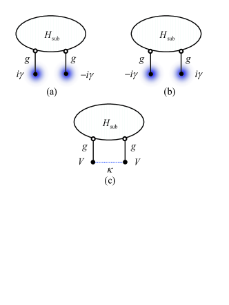
Figure 1: Schematic illustration of configurations for non-Hermitian models and their Hermitian correspondence. (a) is the graph for a non-Hermitian Hamiltonian $\mathcal{H}$, where $H_{\text{{sub}}}$ is an arbitrary Hermitian sub-system. (b) is the graph for the non-Hermitian Hamiltonian $\mathcal{H}^{{\dagger}}$. (c) is the corresponding Hermitian graph, which may have a connection with $\mathcal{H}$ and $\mathcal{H}^{{\dagger}}$.

We start our investigation by considering a class of Hermitian and non-Hermitian Hamiltonians $\{H,\mathcal{H},\mathcal{H}^{{\dagger}}\}$, which consist of two parts

$$\mathcal{H} = H_{\text{{sub}}}+H_{\gamma},$$ (1)

$$H = H_{\text{{sub}}}+H_{\kappa}.$$ (2)

The structure of the systems is schematically illustrated in Fig. 1. Here $H_{\text{{sub}}}$ describes a Hermitian tight-binding Hamiltonian on an arbitrary graph, and non-Hermitian term $H_{\gamma}$ and Hermitian term $H_{\kappa}$ are in the form

$$H_{\gamma} = g(\left|a\right\rangle\left\langle A\right|+\left|b\right\rangle\left\langle B\right|+\mathrm{H.c.})$$ (3)

$$-i\gamma\left|A\right\rangle\left\langle A\right|+i\gamma\left|B\right\rangle\left\langle B\right|$$

and

$$H_{\kappa}=g(\left|a\right\rangle\left\langle A\right|+\left|b\right\rangle\left\langle B\right|+\mathrm{H.c.})$$

$$+\kappa(\left|A\right\rangle\left\langle B\right|+\mathrm{H.c.})+V(\left|A\right\rangle\left\langle A\right|+\left|B\right\rangle\left\langle B\right|),$$ (4)

where $\left|a\right\rangle$ $(\left|b\right\rangle)$ and $\left|A\right\rangle$ $(\left|B\right\rangle)$ are the position states at sites $a$ $(b)$ in $H_{\text{{sub}}}$ and $A$ $(B)$, respectively. In this paper, the hopping integral $\kappa$ and on-site potential $V$ are real. The wave functions of Hamiltonians $\{H,\mathcal{H},\mathcal{H}^{{\dagger}}\}$ are in the forms

$$\left|\eta\right\rangle=\left|\eta_{\mathrm{sub}}\right\rangle+\eta_{a}\left|a\right\rangle+\eta_{b}\left|b\right\rangle+\eta_{A}\left|A\right\rangle+\eta_{B}\left|B\right\rangle,$$ (5)

where $\eta=\psi$, $\varphi$, and $\phi$ denotes the wave functions in the three systems.

The Schrödinger equations with the same real eigenenergy $\varepsilon$ are $H\left|\psi\right\rangle=\varepsilon\left|\psi\right\rangle$, $\mathcal{H}\left|\varphi\right\rangle=\varepsilon\left|\varphi\right\rangle$, and $\mathcal{H}^{{\dagger}}\left|\phi\right\rangle=\varepsilon\left|\phi\right\rangle$, which have the explicit forms

$$\left\{\begin{array}[]{c}H_{\text{{sub}}}\left|\psi_{\mathrm{sub}}\right\rangle=\varepsilon\left|\psi_{\mathrm{sub}}\right\rangle\\ g\psi_{a}-\varepsilon\psi_{A}+V\psi_{A}+\kappa\psi_{B}=0\\ g\psi_{b}-\varepsilon\psi_{B}+V\psi_{B}+\kappa\psi_{A}=0\end{array}\right.,$$ (6)

and

$$\left\{\begin{array}[]{c}H_{\text{{sub}}}\left|\varphi_{\mathrm{sub}}\right\rangle=\varepsilon\left|\varphi_{\mathrm{sub}}\right\rangle\\ g\varphi_{a}-\varepsilon\varphi_{A}-i\gamma\varphi_{A}=0\\ g\varphi_{b}-\varepsilon\varphi_{B}+i\gamma\varphi_{B}=0\end{array}\right.,$$ (7)

and

$$\left\{\begin{array}[]{c}H_{\text{{sub}}}\left|\phi_{\mathrm{sub}}\right\rangle=\varepsilon\left|\phi_{\mathrm{sub}}\right\rangle\\ g\phi_{a}-\varepsilon\phi_{A}+i\gamma\phi_{A}=0\\ g\phi_{b}-\varepsilon\phi_{B}-i\gamma\phi_{B}=0\end{array}\right.,$$ (8)

respectively. Combining the above two equations, we have

$$\left\{\begin{array}[]{c}H_{\text{{sub}}}(\left|\varphi_{\mathrm{sub}}\right\rangle+\left|\phi_{\mathrm{sub}}\right\rangle)=\varepsilon(\left|\varphi_{\mathrm{sub}}\right\rangle+\left|\phi_{\mathrm{sub}}\right\rangle)\\ g(\varphi_{a}+\phi_{a})-\varepsilon(\varphi_{A}+\phi_{A})-i\gamma(\varphi_{A}-\phi_{A})=0\\ g(\varphi_{b}+\phi_{b})-\varepsilon(\varphi_{B}+\phi_{B})+i\gamma(\varphi_{B}-\phi_{B})=0\end{array}\right..$$ (9)

Comparing the Eqs. (6) and (9), we find that one can have

$$\left|\psi\right\rangle=\left|\varphi\right\rangle+\left|\phi\right\rangle,$$ (10)

if the following conditions are satisfied

$$\left\{\begin{array}[]{c}V\psi_{A}+\kappa\psi_{B}=-i\gamma(\varphi_{A}-\phi_{A})\\ V\psi_{B}+\kappa\psi_{A}=i\gamma(\varphi_{B}-\phi_{B})\end{array}\right.,$$ (11)

From Eq. (10), we have

$$\psi_{A}=\varphi_{A}+\phi_{A},\text{ }\psi_{B}=\varphi_{B}+\phi_{B}.$$ (12)

Submitting the above equations into Eq. (11), we have

$$\left(\begin{array}[]{c}\varphi_{A}\\ \varphi_{B}\end{array}\right)=-\frac{V+\kappa\sigma_{x}-i\gamma\sigma_{z}}{V+\kappa\sigma_{x}+i\gamma\sigma_{z}}\left(\begin{array}[]{c}\phi_{A}\\ \phi_{B}\end{array}\right),$$ (13)

where $\sigma_{x}$ and $\sigma_{x}$ are Pauli matrices. It indicates that the solutions of $\varphi_{A,B}$ and $\phi_{A,B}$ for a given $\gamma$ may lead to the restriction on parameters $V$ and $\kappa$.

In this work, the non-Hermiticity arises from the imaginary potentials. Then we have $\mathcal{H}^{{\dagger}}=\mathcal{H}^{\ast}$, which allows us to write the eigenfunctions in the form of $\varphi_{A}=\phi_{A}^{\ast}$ and $\varphi_{B}=\phi_{B}^{\ast}$ for real-energy eigenstates. Therefore the above equation can be reduced as

$$(V+\kappa\sigma_{x})\left(\begin{array}[]{c}\text{Re}\varphi_{A}\\ \text{Re}\varphi_{B}\end{array}\right)=\gamma\sigma_{z}\left(\begin{array}[]{c}\text{Im}\varphi_{A}\\ \text{Im}\varphi_{B}\end{array}\right),$$ (14)

or the explicit form

$$\left\{\begin{array}[]{c}V\text{Re}\varphi_{A}+\kappa\text{Re}\varphi_{B}-\gamma\text{Im}\varphi_{A}=0\\ \kappa\text{Re}\varphi_{A}+V\text{Re}\varphi_{B}+\gamma\text{Im}\varphi_{B}=0\end{array}\right.,$$ (15)

based on which one can establish the relation among $V$, $\kappa$, and $\gamma$. We see that the relation depends on the eigenstates of $\mathcal{H}$.

For a $\mathcal{PT}$-symmetric system, which corresponds to parity symmetric $H_{\text{{sub}}}$, a real-energy state can always be written as the form of $\varphi_{A}=\pm\varphi_{B}^{\ast}$, i.e., Re$\varphi_{A}=\pm$Re$\varphi_{B}$ and Im$\varphi_{A}=\mp$Im$\varphi_{B}$. This leads to

$$\left(V\pm\kappa\right)\text{Re}\varphi_{A}-\gamma\text{Im}\varphi_{A}=0,$$ (16)

which means that the Hermitian Hamiltonian is $\gamma$-dependent. Furthermore, for a simpler case with real $\varphi_{A}$ and $\varphi_{B}$, the fact Im$\varphi_{A,B}=0$ leads to

$$\kappa=\pm V,$$ (17)

and

$$\varphi_{A}=\phi_{A}=\psi_{A}/2=\mp\varphi_{B}=\mp\phi_{B}=\mp\psi_{B}/2,$$ (18)

correspondingly. Therefore if one can find a non-Hermitian system $\mathcal{H}$, which has an eigenvector with real components $\varphi_{A}=\mp\varphi_{B}$, there should exist a Hermitian system $H$ with $\kappa=\pm V$ and there must have an eigenvector in the form of Eq. (10). And the two eigenvectors have the same real eigenvalue.

Finally, it is necessary to stress that the relation expressed in Eq. (10) is subtle. If one find that the superposition $\left|\varphi\right\rangle+\left|\phi\right\rangle$ corresponds to an eigenstate $\left|\psi\right\rangle=\left|\varphi\right\rangle+\left|\phi\right\rangle$ of a Hamiltonian $H$, another superposition $\alpha\left|\varphi\right\rangle+\beta\left|\phi\right\rangle$ may correspond to an eigenstate $\left|\psi^{\prime}\right\rangle=\alpha\left|\varphi\right\rangle+\beta\left|\phi\right\rangle$ of another Hamiltonian $H^{\prime}$. Nevertheless, all four states $\left|\varphi\right\rangle,$ $\left|\phi\right\rangle,$ $\left|\psi\right\rangle$, and $\left|\psi^{\prime}\right\rangle$ have the same eigenvalue with respect to their own Hamiltonians $\mathcal{H},$ $\mathcal{H}^{{\dagger}},$ $H$, and $H^{\prime}$, respectively.

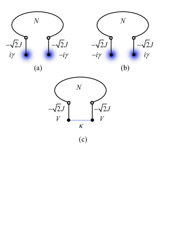
Figure 2: Schematic illustrations for the uniform chain. Here $H_{\text{{sub}}}$ is a uniform chain of length $N$. Exact solution shows that the combination of eigenstates of systems (a) and (b) is also the eigenstate of system (c) under the condition $\kappa=\pm V$.

3 Illustrative examples

3.1 Uniform chain

In this section, we investigate a simple and exactly solvable system to illustrate the main idea of our paper. In order to exemplify the above mentioned analysis of connecting the eigenstate of $H$ to those of $\mathcal{H}$ and $\mathcal{H}^{{\dagger}}$, we take $H_{\text{sub}}$ to be the simplest network: a uniform chain. The sub-Hamiltonian in the sample Hamiltonian has the form

$$H_{\text{sub}}=-J\overset{N-1}{\sum_{l=1}}\left(\left|l\right\rangle\left\langle l+1\right|+\mathrm{H.c.}\right),$$ (19)

and non-Hermitian term

$$H_{\gamma} = -\sqrt{2}J(\left|1\right\rangle\left\langle A\right|+\left|N\right\rangle\left\langle B\right|+\mathrm{H.c.})$$ (20)

$$-i\gamma\left|A\right\rangle\left\langle A\right|+i\gamma\left|B\right\rangle\left\langle B\right|,$$

and Hermitian term

$$H_{\kappa}=-\sqrt{2}J(\left|1\right\rangle\left\langle A\right|+\left|N\right\rangle\left\langle B\right|+\mathrm{H.c.})$$

$$+\kappa(\left|A\right\rangle\left\langle B\right|+\mathrm{H.c.})+V(\left|A\right\rangle\left\langle A\right|+\left|B\right\rangle\left\langle B\right|),$$ (21)

which are sketched in Fig. 2. We note that $\mathcal{H}$($\mathcal{H}^{{\dagger}}$) has $\mathcal{PT}$ symmetry, i.e., $\mathcal{PTH(\mathcal{H}^{{\dagger}})}(\mathcal{PT})^{-1}=\mathcal{H}$($\mathcal{H}^{{\dagger}}$), which was proposed and exactly solved in Ref. [19]. Here $\mathcal{P}$ and $\mathcal{T}$ represent the space-reflection operator (or parity operator) and the time-reversal operator, respectively. The corresponding Hermitian Hamiltonian $H$ has both $\mathcal{P}$ and $\mathcal{T}$ symmetries.

To demonstrate our result, we consider the solutions of the Hamiltonians with $N=2$. On the basis $\{\left|A\right\rangle,$ $\left|l=1,2\right\rangle,$ $\left|B\right\rangle\}$, the Hamiltonians can be written as

$$H=J\left(\begin{array}[]{cccc}V/J&-\sqrt{2}&0&\kappa/J\\ -\sqrt{2}&0&-1&0\\ 0&-1&0&-\sqrt{2}\\ \kappa/J&0&-\sqrt{2}&V/J\end{array}\right),$$ (22)

and

$$\mathcal{H}=\mathcal{H}^{{\dagger}}(-\gamma)$$ (27)

$$= J\left(\begin{array}[]{cccc}-i\gamma/J&-\sqrt{2}&0&0\\ -\sqrt{2}&0&-1&0\\ 0&-1&0&-\sqrt{2}\\ 0&0&-\sqrt{2}&i\gamma/J\end{array}\right).$$

Our goal is to present the connections between them. To this end, the relevant eigenvectors and eigenvalues of $\mathcal{H}$ (as well as $\mathcal{H}^{{\dagger}}$) can be exactly obtained as

$$\varphi_{1,2}=\left(\begin{array}[]{c}\left(a_{\pm}^{\ast}\right)^{3}\\ \sqrt{2}a_{\pm}^{\ast}\\ \sqrt{2}a_{\pm}\\ a_{\pm}^{3}\end{array}\right),\varepsilon_{1,2}=\varepsilon_{\pm}=\pm J\sqrt{4-\gamma^{2}}$$ (28)

and

$$\varphi_{3,4} = \left(\begin{array}[]{c}-1\\ \frac{\sqrt{2}}{2}\left(i\gamma/J-1\right)\\ \frac{\sqrt{2}}{2}\left(i\gamma/J+1\right)\\ 1\end{array}\right),\left(\begin{array}[]{c}1\\ -\frac{\sqrt{2}}{2}\left(i\gamma/J+1\right)\\ \frac{\sqrt{2}}{2}\left(i\gamma/J-1\right)\\ 1\end{array}\right),$$ (37)

$$\varepsilon_{3} = -\varepsilon_{4}=-J,$$ (38)

where the complex numbers are

$$a_{\pm}=\sqrt{2}(i\gamma/J-\varepsilon_{\pm})^{-1/2}.$$ (39)

Here the eigenvectors are written as $\mathcal{PT}$-symmetric form, i.e., $\mathcal{PT}\left|\varphi_{i}\right\rangle=\left|\varphi_{i}\right\rangle$.

And the eigenvectors and eigenvalues of $H$ can also be exactly obtained as

$$\psi_{\lambda+} = \frac{1}{2}\left(\begin{array}[]{c}-e_{\lambda\pm}/J\mp 1\\ \sqrt{2}\\ \pm\sqrt{2}\\ \mp e_{\lambda\pm}/J-1\end{array}\right),\lambda=1,2,$$ (44)

$$e_{\lambda\pm} = \frac{1}{2}\{[V\pm\left(\kappa-J\right)]$$ (45)

$$+\left(-1\right)^{\lambda}\sqrt{\left(V-\kappa-J\right)^{2}+8J^{2}}\},$$

Here the states $\left\{\varphi_{i},i=1,2,3,4\right\}$ are also eigenstates of the $\mathcal{PT}$ operator. Now we apply our conclusion, i.e., Eq. (16), on states $\left\{\varphi_{i}\right\}$ one by one and demonstrate the main point.

(i) $\varphi_{1}:$ For this state, Eq. (16) tells us

$$V+\kappa=\frac{\gamma^{2}(\sqrt{4-\gamma^{2}}+1)}{(\sqrt{4-\gamma^{2}}+2)(\sqrt{4-\gamma^{2}}-1)},$$ (46)

which yields

$$\psi_{1+}=\frac{1}{2}\left(\begin{array}[]{c}-e_{1+}-1\\ \sqrt{2}\\ \sqrt{2}\\ -e_{1+}-1\end{array}\right),e_{1+}=-\sqrt{4-\gamma^{2}},$$ (47)

for $\gamma^{2}\leqslant 3$. Then we have the relation

$$\varphi_{1}+\phi_{1}=2(\sqrt{4-\gamma^{2}}+2)^{1/2}\psi_{1+}.$$ (48)

On the other hand, if $\gamma^{2}\geqslant 3$, we get

$$\psi_{2+}=\frac{1}{2}\left(\begin{array}[]{c}-e_{2+}-1\\ \sqrt{2}\\ \sqrt{2}\\ -e_{2+}-1\end{array}\right),e_{2+}=-\sqrt{4-\gamma^{2}},$$ (49)

which results in

$$\varphi_{1}+\phi_{1}=2(\sqrt{4-\gamma^{2}}+2)^{1/2}\psi_{2+}.$$ (50)

(ii) $\varphi_{2}:$ For this state, by the similar procedure, we obtain

$$\varphi_{2}+\phi_{2}=2(2-\sqrt{4-\gamma^{2}})^{1/2}\psi_{2+},$$ (51)

for $\gamma^{2}\leqslant 3$ and

$$\varphi_{2}+\phi_{2}=2(2-\sqrt{4-\gamma^{2}})^{1/2}\psi_{1+},$$ (52)

for $\gamma^{2}\geqslant 3$, respectively.

(iii) $\varphi_{3}:$ For this state, Eq. (15) tells us $V=\kappa$, which leads to

$$\psi_{1-}=\frac{1}{\sqrt{2}}\left(\begin{array}[]{c}\sqrt{2}\\ 1\\ -1\\ -\sqrt{2}\end{array}\right),e_{1-}=-1,$$ (53)

and

$$\varphi_{3}+\phi_{3}=-2\psi_{1-}.$$ (54)

(iv) $\varphi_{4}:$ For this state, Eq. (16) tells us $V=-\kappa$, which leads to

$$\psi_{2+}=\frac{1}{\sqrt{2}}\left(\begin{array}[]{c}-\sqrt{2}\\ 1\\ 1\\ -\sqrt{2}\end{array}\right),e_{2+}=1,$$ (55)

and correspondingly

$$\varphi_{4}+\phi_{4}=-2\psi_{2+}.$$ (56)

Based on the explicit solutions, we conclude that for a given $\gamma$, $\varphi_{i}+\phi_{i}$, a superposition of real-energy eigenstates of $\mathcal{H}$ and $\mathcal{H}^{{\dagger}}$, always corresponds to an eigenstate $\psi_{j}$ of $H$, i.e.,

$$\varphi_{i}+\phi_{i}\propto\psi_{j},$$ (57)

with the same eigenenergy. These facts demonstrate and verify our analysis in the last section. Moreover, it also has an implication that one can find the corresponding Hermitian Hamiltonian for every state $\varphi_{i}+\phi_{i}$.

For large $N$, it is a little difficult to give analytical expressions of eigenstates for arbitrary parameters. Fortunately, we can provide some eigenstates for specific parameters. We consider the case with $N=4m+3$ ($m$ is an integer), $\gamma=\pm 2J$, and $\kappa=V$. For non-Hermitian Hamiltonians $\mathcal{H}$ and $\mathcal{H}^{{\dagger}}$, there is a zero-energy state, which is the coalescing state of three levels with eigenenergies $0$, and $\pm\sqrt{4J^{2}-\gamma^{2}}$ for $\gamma^{2}\leqslant 4J^{2}$, respectively. The eigenstates of $\mathcal{H}$ and $\mathcal{H}^{{\dagger}}$ can be written as

$$\left|\Phi_{-}\right\rangle = \left|\Phi_{+}\right\rangle^{\ast}=\frac{1}{\sqrt{2\left(N-1\right)}}[\left|A\right\rangle$$ (58)

$$-i^{N+1}\left|B\right\rangle-\sqrt{2}\sum_{l=2}^{N-1}i^{l+1}\left|l\right\rangle],$$

which can be checked to satisfy $\mathcal{H}\left|\Phi_{-}\right\rangle=\mathcal{H}^{{\dagger}}\left|\Phi_{+}\right\rangle=0$ and $\langle\Phi_{\pm}\left|\Phi_{\pm}\right\rangle=1$. We note that the biorthogonal norm of $\left|\Phi_{\pm}\right\rangle$ is

$$\langle\Phi_{+}\left|\Phi_{-}\right\rangle=0,$$ (59)

which indicates that it is a coalescing state. On the other hand, the zero-energy state of $H$ is

$$\left|\Psi\right\rangle=\frac{1}{\sqrt{N-1}}(\sum_{j=2}^{N-1}\sin\frac{\pi j}{2}\left|j\right\rangle+\sqrt{2}\left|1\right\rangle-\sqrt{2}\left|N\right\rangle),$$ (60)

which satisfies $H\left|\Psi\right\rangle=0$. And it is easy to check that

$$\left|\Psi\right\rangle=\left|\Phi_{+}\right\rangle+\left|\Phi_{-}\right\rangle.$$ (61)

The physical picture of this relation is clear: states $\left|\Phi_{+}\right\rangle$ and $\left|\Phi_{-}\right\rangle$ represent two plane waves with wave vectors $\pm\pi/2$, while state $\left|\Psi\right\rangle$ stands for a standing wave.

3.2 Su-Schrieffer-Heeger chain

In this section, we present another example to show the application of above conclusion for quantum engineering. We take $H_{\text{sub}}$ to be an SSH chain, which is proposed by Su, Schrieffer, and Heeger (SSH) to model polyacetylene [20, 21], is the prototype of a topologically nontrivial band insulator with a symmetry protected topological phase [22, 23]. In recent years, it has been attracted much attention and extensive studies have been demonstrated [24, 25, 26, 27, 28, 29]. The sub-Hamiltonian in this example is

$$H_{\text{sub}} = -\left(J-J\delta\right)\sum_{j=1}^{N/2}\left|2j-1\right\rangle\left\langle 2j\right|$$ (63)

$$-\left(J+J\delta\right)\sum_{j=1}^{N/2-j}\left|2j\right\rangle\left\langle 2j+1\right|+\mathrm{H.c.},$$

and non-Hermitian term is

$$H_{\gamma}=-i\gamma\left(\left|1\right\rangle\left\langle 1\right|-\left|N\right\rangle\left\langle N\right|\right),$$ (64)

and Hermitian term is

$$H_{\kappa}=-\kappa(\left|1\right\rangle\left\langle N\right|+\mathrm{H.c.}),$$ (65)

which are sketched in Fig. 3. We note that $\mathcal{H}$($\mathcal{H}^{{\dagger}}$) also has $\mathcal{PT}$ symmetry. It is tough to give an explicit form of the eigenstates. Fortunately, exact zero-mode eigenstates of both $H$ and $\mathcal{H}$($\mathcal{H}^{{\dagger}}$) are obtained for specific relation among $\gamma$, $\delta$ and $\kappa$ [30]. For Hamiltonian $H$, there are two degenerate zero-mode eigenstates, which has the form

$$\left|\psi_{\pm}\right\rangle=\Omega\sum_{j=1}^{N/2}[\left(-\Delta\right)^{j-1}\left|2j-1\right\rangle\pm\left(-\Delta\right)^{N/2-j}\left|2j\right\rangle],$$ (66)

$$\left|\psi_{1}\right\rangle = \sqrt{2}\Omega\sum_{j=1}^{N/2}\left(-\Delta\right)^{j-1}\left|2j-1\right\rangle,$$ (67)

$$\left|\psi_{2}\right\rangle = \sqrt{2}\Omega\sum_{j=1}^{N/2}\left(-\Delta\right)^{N/2-j}\left|2j\right\rangle,$$ (68)

satisfying

$$H\left(\kappa_{\mathrm{c}}\right)\left|\psi_{1}\right\rangle=[H\left(\kappa_{\mathrm{c}}\right)]^{\dagger}\left|\psi_{2}\right\rangle=0.$$ (69)

and

$$\kappa=\kappa_{\mathrm{c}}=J(1+\delta)\Delta^{N/2},$$ (70)

where $\Delta=\left(1-\delta\right)/\left(1+\delta\right)$ denotes the staggered hopping strength and $\Omega=\sqrt{2\delta J^{2}/(J^{2}(1+\delta)^{2}-\kappa^{2})}$ is the Dirac normalizing constant. For non-Hermitian Hamiltonian $\mathcal{H}$($\mathcal{H}^{{\dagger}}$), the zero-mode state is a coalescence state

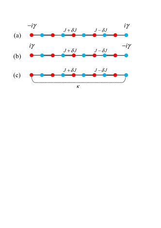
Figure 3: Schematic illustrations for the SSH chain. Here $H_{\text{{sub}}}$ is an SSH chain of length $N$. The combination of zero-mode eigenstates of systems (a) and (b) is also zero-mode eigenstate of system (c) under the condition $\kappa=\gamma=J\left(1+\delta\right)\Delta^{N/2},\Omega=\sqrt{2\delta J^{2}/(J^{2}(1+\delta)^{2}-\kappa^{2})}$.

$$\left|\varphi_{\mathrm{zm}}\right\rangle=\Omega\sum_{j=1}^{N/2}[\left(-\Delta\right)^{j-1}\left|2j-1\right\rangle+i\left(-\Delta\right)^{N/2-j}\left|2j\right\rangle]\left|\text{{vac}}\right\rangle,$$ (71)

Similarly, the zero-mode state for $H_{\gamma_{\mathrm{c}}}^{\dagger}$ can be constructed as

$$\left|\eta_{\mathrm{zm}}\right\rangle=\Omega\sum_{j=1}^{N/2}[\left(-\Delta\right)^{j-1}\left|2j-1\right\rangle-i\left(-\Delta\right)^{N/2-j}\left|2j\right\rangle]\left|\text{{vac}}\right\rangle,$$ (72)

satisfying

$$H\left(\gamma_{\mathrm{c}}\right)\left|\varphi_{\mathrm{zm}}\right\rangle=[H\left(\gamma_{\mathrm{c}}\right)]^{\dagger}\left|\eta_{\mathrm{zm}}\right\rangle=0.$$ (73)

and

$$\gamma=\gamma_{\mathrm{c}}=\kappa_{\mathrm{c}}=J(1+\delta)\Delta^{N/2},$$ (74)

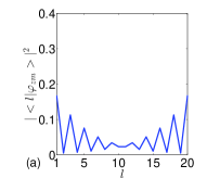
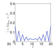
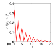
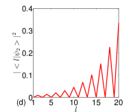
Figure 4: The Dirac probabilities of the four zero-mode eigstates for SSH model in Fig. 4(a-c) at $\delta=0.1,N=20$. (a) $\langle\varphi_{\mathrm{zm}}\left|\varphi_{\mathrm{zm}}\right\rangle$, (b) $\langle\eta_{\mathrm{zm}}\left|\eta_{\mathrm{zm}}\right\rangle$, (c) $\langle\psi_{1}\left|\psi_{1}\right\rangle$, (d) $\langle\psi_{2}\left|\psi_{2}\right\rangle$.

Three wave functions for finite $N=20$ are plotted in Fig. 4. They satisfies the following relations

$$\left|\varphi_{\mathrm{zm}}\right\rangle+\left|\eta_{\mathrm{zm}}\right\rangle = \sqrt{2}\left|\psi_{1}\right\rangle,$$

$$\left|\varphi_{\mathrm{zm}}\right\rangle-\left|\eta_{\mathrm{zm}}\right\rangle = \sqrt{2}\left|\psi_{2}\right\rangle.$$

The first relationship is accords with our previous conclusion, which shows a symmetric combination under relation $\left|\varphi_{\mathrm{zm}}\right\rangle+\left|\eta_{\mathrm{zm}}\right\rangle$; the second relationship shows an anti-symmetric combination of the eigen states under relation $\left|\varphi_{\mathrm{zm}}\right\rangle-\left|\eta_{\mathrm{zm}}\right\rangle$. The results of two concrete examples show that our general conclusion is feasible in practice.

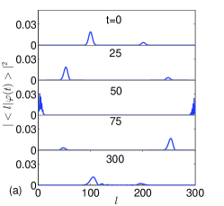
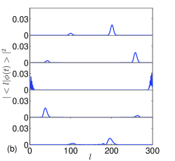
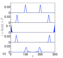
Figure 5: The time evolution profiles of three initial states with the same distribution in Eq. (92) with $\alpha=0.2$, the evolutions are governed by their own systems. (a) The initial state state $\left|\varphi(0)\right\rangle$ is in $\mathcal{H}$, (b) The initial state $\left|\phi(0)\right\rangle$ is in $\mathcal{H}^{{\dagger}}$, (c) The initial state $\left|\psi\left(0\right)\right\rangle$ or $\left|\varphi(0)\right\rangle+\left|\phi(0)\right\rangle$ in $H$. The unit of time is $1/J$. The plots are taken for five typical instants. In (c), $\left|\left|\psi\left(t\right)\right\rangle\right|^{2}$ is plotted in order to compare with that in (a) and (b).

4 Parallel dynamics

In this section, we apply the obtained results on the dynamics of the relevant Hamiltonians. In the above section, we have shown that there exist three sets of eigenstates $\left\{\left|\psi_{n}\right\rangle\right\}$, $\left\{\left|\varphi_{n}\right\rangle\right\}$, and $\left\{\left|\phi_{n}\right\rangle\right\}$ for the Hamiltonians $H$, $\mathcal{H}$, and $\mathcal{H}^{{\dagger}}$, respectively, which obey the relation $\left|\psi_{n}\right\rangle=\left|\varphi_{n}\right\rangle+\left|\phi_{n}\right\rangle$. The three sets of eigenstates have the same eigenenergies $\left\{\varepsilon_{n}\right\}$. Now we consider the time evolution of an initial state in the subspace $\left\{\left|\psi_{n}\right\rangle\right\}$, i.e.,

$$\left|\psi(0)\right\rangle=\sum_{n}c_{n}\left|\psi_{n}\right\rangle.$$ (75)

The evolved state is

$$\left|\psi(t)\right\rangle = \sum_{n}c_{n}e^{-i\varepsilon_{n}t}\left|\psi_{n}\right\rangle$$ (76)

$$= e^{-i\mathcal{H}t}\left|\varphi(0)\right\rangle+e^{-i\mathcal{H}^{{\dagger}}t}\left|\phi(0)\right\rangle,$$

where

$$\left|\varphi(0)\right\rangle=\sum_{n}c_{n}\left|\varphi_{n}\right\rangle,\left|\phi(0)\right\rangle=\sum_{n}c_{n}\left|\phi_{n}\right\rangle.$$ (77)

It indicates that, for a dynamic process $\left|\varphi(t)\right\rangle$ in a non-Hermitian system $\mathcal{H}$, there always exists a parallel dynamic process $\left|\phi(t)\right\rangle$ governed by the corresponding Hermitian conjugate Hamiltonian $\mathcal{H}^{{\dagger}}$. And it is shown that a linear superposition of the two parallel dynamics may be exactly equivalent to the time evolution of a state $\left|\psi(t)\right\rangle$ under a Hermitian Hamiltonian $H$.

Furthermore, we note that, the total Dirac probabilities of three states obey the relations

$$\langle\psi(t)\left|\psi(t)\right\rangle=\langle\varphi(t)\left|\varphi(t)\right\rangle+\langle\phi(t)\left|\phi(t)\right\rangle+2\theta,$$ (78)

and

$$\frac{\text{d}}{\text{d}t}\left|\left|\varphi(t)\right\rangle\right|^{2}+\frac{\text{d}}{\text{d}t}\left|\left|\phi(t)\right\rangle\right|^{2}=\frac{\text{d}}{\text{d}t}\left|\left|\psi(t)\right\rangle\right|^{2}=0,$$ (79)

due to the biorthonormal relation

$$\frac{1}{\theta}\langle\varphi(t)\left|\phi(t)\right\rangle=\frac{1}{\theta}\langle\varphi(t)\left|\phi(t)\right\rangle=1,$$ (80)

where $\theta$ is a constant.

Specifically, when the system is $\mathcal{PT}$-symmetric and $\mathcal{H}^{{\dagger}}=\mathcal{H}^{\ast}$, we have $\mathcal{PHP}^{-1}=\mathcal{H}^{{\dagger}}$. We note that operation $\mathcal{P}$ cannot affect the Dirac probability, i.e., $\left|\left|\varphi(t)\right\rangle\right|^{2}=\left|\left|\phi(t)\right\rangle\right|^{2}$. Then we have

$$\frac{\text{d}}{\text{d}t}\left|\left|\varphi(t)\right\rangle\right|^{2}=\frac{\text{d}}{\text{d}t}\left|\left|\phi(t)\right\rangle\right|^{2}=0,$$ (81)

i.e., the Dirac probabilities of the two states are conservative. In general, a non-Hermitian system obeys the conservation of biorthogonal probability rather than Dirac probability. However, in the sub-sets $\left\{\left|\varphi_{n}\right\rangle\right\}$ and $\left\{\left|\phi_{n}\right\rangle\right\}$, both types of probability are conservative.

Next we demonstrate this feature by the numerical simulation of the time evolution of a specific initial state under a concrete system. We consider the Hamiltonians $H$, $\mathcal{H}$, and $\mathcal{H}^{{\dagger}}$, which consist of sub-Hamiltonians $H_{\text{sub}}$, $H_{\gamma}$, and $H_{\kappa}$ defined in Eqs. (19), (20), and (21), respectively. Here the parameters are taken as $N=300$, $\gamma=0.75$, and $\kappa=-V=-1$. In this case, an exact eigenstate can be obtained as

$$\left|\psi_{0}\right\rangle = \frac{1}{\sqrt{2\left(N-1\right)}}\left(\overset{N-1}{\underset{l=2}{\sum}}\sqrt{2}\left|l\right\rangle+\left|1\right\rangle+\left|N\right\rangle\right)$$ (82)

$$\varepsilon_{0} = -2J.$$ (83)

On the other hand, numerical result shows that there are three $149$-dimensional sets of eigenstates $\{H:\left|\psi_{m}\right\rangle\}$, $\{\mathcal{H}:\left|\varphi_{m}\right\rangle\}$, and $\{\mathcal{H}^{{\dagger}}:\left|\phi_{m}\right\rangle\}$, which have the identical eigenenergies $\left\{\varepsilon_{m}\right\}$, $m\in[1,149]$. State $\left|\psi_{0}\right\rangle$ is not included in the set $\{\left|\psi_{m}\right\rangle\}$. These states satisfy

$$\mathcal{P}\left|\psi_{m}\right\rangle = \left|\psi_{m}\right\rangle,$$ (84)

$$\mathcal{PT}\left|\varphi_{m}\right\rangle = \left|\varphi_{m}\right\rangle,$$ (85)

$$\mathcal{PT}\left|\phi_{m}\right\rangle = \left|\phi_{m}\right\rangle,$$ (86)

and can be written as the form

$$\langle A\left|\varphi_{m}\right\rangle = \langle A\left|\phi_{m}\right\rangle=\langle A\left|\psi_{m}\right\rangle/2$$ (87)

$$= \langle B\left|\varphi_{m}\right\rangle=\langle B\left|\phi_{m}\right\rangle=\langle B\left|\psi_{m}\right\rangle/2.$$ (88)

Then we have the relation $\left|\psi_{m}\right\rangle=\left|\varphi_{m}\right\rangle+\left|\phi_{m}\right\rangle$. Based on these analyses, we find that an arbitrary state $\left|\psi\left(0\right)\right\rangle$ satisfying

$$\mathcal{P}\left|\psi\left(0\right)\right\rangle=\left|\psi\left(0\right)\right\rangle,\langle\psi_{0}\left|\psi\left(0\right)\right\rangle=0,$$ (89)

can be the state exhibiting the parallel dynamics. In this paper, we consider an Gaussian wave packet

$$\left|N/3,\pi/2\right\rangle=\frac{1}{\sqrt{\Omega}}\sum_{j}e^{-\alpha^{2}\left(j-N/3\right)^{2}}e^{i\pi/2j}\left|j\right\rangle.$$ (90)

Here $\Omega=\sqrt{\pi/2}/\alpha$ is the normalization factor and $\sqrt{2\ln 2}/\alpha\ll N/2$ is the width of the wave packet. We take the central momentum of the wave packet as $\pi/2$, which weeds out the component of state $\left|\psi_{0}\right\rangle$. The initial state is constructed as

$$\left|\psi\left(0\right)\right\rangle=\frac{1}{\sqrt{2}}(\left|N/3,\pi/2\right\rangle+\mathcal{P}\left|N/3,\pi/2\right\rangle),$$ (91)

which is spanned by the set $\{\left|\psi_{m}\right\rangle\}$ with the coefficient

$$c_{n}=\langle\psi_{n}\left|\psi\left(0\right)\right\rangle.$$ (92)

Based on $\{c_{n}\}$, the initial states $\left|\varphi(0)\right\rangle$ and $\left|\phi(0)\right\rangle$ can be obtained accordingly. We compute the time evolutions of states $\left|\psi\left(0\right)\right\rangle$, $\left|\varphi(0)\right\rangle$, and $\left|\phi(0)\right\rangle$ by exact diagonalizations. Plots of Dirac probabilities $\left|\langle l\left|\varphi(t)\right\rangle\right|^{2}$, $\left|\langle l\left|\phi(t)\right\rangle\right|^{2}$, and $\left|\langle l\left|\psi(t)\right\rangle\right|^{2}$ of the evolved states at several typical instants are listed in Fig. 5. The profiles of initial states are two separated symmetric Gaussian wave packets for $H$ but asymmetric for $\mathcal{H}$ and $\mathcal{H}^{{\dagger}}$. At beginning, three initial states evolve in the same way before they collide with the boundaries. It is due to the fact that three Hamiltonians $H$, $\mathcal{H}$, and $\mathcal{H}^{{\dagger}}$ contain the same sub-Hamiltonian $H_{\text{sub}}$. When the wave packets reach the boundaries, the imaginary potentials are taking effect. The positive imaginary potentials increase the probabilities, while the negative ones decrease the probabilities, violating the conservation of probabilities of each individual wave packet. In contrast, the profile of $\left|\langle l\left|\psi(t)\right\rangle\right|^{2}$ or $\left|\left\langle l\right|[\left|\varphi(t)\right\rangle+\left|\phi(t)\right\rangle]\right|^{2}$ exhibits a Hermitian dynamical behavior. Two symmetric wave packets collide with each other at the joint. According to the analysis above, the total Dirac probabilities of states $\left|\varphi(t)\right\rangle$ and $\left|\phi(t)\right\rangle$ are still conservative. This non-intuitive behavior arises from the asymmetry of two wave packets. The gain of the small wave packet counteracts the loss of the big one.

5 Conclusion and discussion

In conclusion, we have presented a novel way of finding the link between a non-Hermitian Hamiltonian and a Hermitian one, based on the exact solutions. We have found that there is a class of non-Hermitian Hamiltonians which has a subtle relation to a class of Hermitian Hamiltonians. Unlike the previous works, the connection refers to all the eigenenergies and eigenvectors of three Hamiltonians. The correspondence among the three Hamiltonians is not only for an individual state but a subset of eigenstates. The identities about eigenvectors and eigenenergies would ensure the identical dynamics. In this work, we just reveal the existence in tractable models (restricted in the systems with imaginary potentials, being probably $\mathcal{PT}$ type). We think the extension to more general models is possible. This finding implies that there may be three parallel worlds around us: an event we observe in our Hermitian world is the combination of two events from the other two non-Hermitian worlds.

References

- [1] C.M. Bender, S. Boettcher, Phys. Rev. Lett. 80 (1998) 5243.
- [2] C.M. Bender, S. Boettcher, P.N. Meisinger, J. Math. Phys. 40 (1999) 2201.
- [3] P. Dorey, C. Dunning, R. Tateo, J. Phys. A: Math. Gen. 34 (2001) L391.
- [4] P. Dorey, C. Dunning, R. Tateo, J. Phys. A: Math. Gen 34 (2001) 5679.
- [5] C.M. Bender, D.C. Brody, H.F. Jones, Phys. Rev. Lett. 89 (2002) 270401.
- [6] A. Mostafazadeh, J. Math. Phys. 43 (2002) 3944.
- [7] A. Mostafazadeh, J. Phys. A: Math. Gen. 36 (2003) 7081.
- [8] H.F. Jones, J. Phys. A: Math. Gen. 38 (2005) 1741.
- [9] M. Znojil, J. Phys. A 40 (2007) 13131.
- [10] M. Znojil, J. Phys. A 41 (2008) 292002.
- [11] M. Znojil, Phys. Rev. A 82 (2010) 052113.
- [12] A. Mostafazadeh, A. Batal, J. Phys. A: Math. Gen. 37 (2004) 11645.
- [13] A. Mostafazadeh, J. Phys. A: Math. Gen. 38 (2005) 6557.
- [14] A. Mostafazadeh, J. Phys. A: Math. Gen. 39 (2006) 10171.
- [15] A. Mostafazadeh, J. Phys. A: Math. Gen. 39 (2006) 13495.
- [16] L. Jin Z. Song, Phys. Rev. A 80 (2009) 052107.
- [17] L. Jin Z. Song, Phys. Rev. A 81 (2010) 032109.
- [18] L. Jin Z. Song, Phys. Rev. A 83 (2011) 062118.
- [19] L. Jin Z. Song, J. Phys. A: Math. Theor. 44 (2011) 375304.
- [20] W.P. Su, J. R. Schrieffer, A. J. Heeger, Phys. Rev. Lett. 42 (1979) 1698.
- [21] J. R. Schrieffer, The Lesson of Quantum Theory, North Holland, Amsterdam, 1986.
- [22] Shinsei Ryu, Yasuhiro Hatsugai, Phys. Rev. Lett. 89 (2002) 077002.
- [23] X.G. Wen, Phys. Rev. B 85 (2012) 085103.
- [24] D. Xiao, M.C. Chang, Q. Niu, Rev. Modern Phys. 82 (2010) 1959.
- [25] M.Z. Hasan, C.L. Kane, Rev. Modern Phys. 82 (2010) 3045.
- [26] X.L. Qi and S.C. Zhang, Rev. Modern Phys. 83 (2011) 1057.
- [27] P. Delplace, D. Ullmo, G. Montambaux, Phys. Rev. B 84 (2011) 195452.
- [28] L.H Li, Z.H Xu, S. Chen, Phys. Rev. B 89 (2014) 085111.
- [29] L.H Li, Z.H Xu, Phys. Rev. B 92 (2015) 085118.
- [30] S. Lin, X.Z. Zhang, C. Li, Z. Song, Phys. Rev. A 94 (2016) 042133.