Enhancement of crossed Andreev reflection in normal-superconductor-normal junction of thin topological insulator

Abstract

We theoretically investigate the subgapped transport phenomena through a normal-superconductor-normal (NSN) junction made up of ultra thin topological insulator with proximity induced superconductivity. The dimensional crossover from three dimensional ($3$D) topological insulator (TI) to thin two-dimensional ($2$D) TI introduces a new degree of freedom, the so-called hybridization or coupling between the two surface states. We explore the role of hybridization in transport properties of the NSN junction, especially how it affects the crossed Andreev reflection (CAR). We observe that a rib-like pattern appears in CAR probability profile while examined as a function of angle of incidence and length of the superconductor. Depending on the incoming and reflection or transmission channel, CAR probability can be maneuvered to be higher than $97\%$ under suitable coupling between the two TI surface states along with appropriate gate voltage and doping concentration in the normal region. Coupling between the two surfaces also induces an additional oscillation envelope in the behavior of the angle averaged conductance, with the variation of the length of the superconductor. The behavior of co-tunneling (CT) probability is also very sensitive to the coupling and other parameters. Finally, we also explore the shot noise cross correlation and show that the behavior of the same can be monotonic or non-monotonic depending on the doping concentration in the normal region. Under suitable circumstances, shot noise cross correlation can change sign from positive to negative or vice versa depending on the relative strength of CT and CAR.

I Introduction

The phenomenon of electron-hole conversion across the interface of a normal metal and superconductor, known as Andreev reflection Andreev (1964)(AR), has been paid much attention in last decade especially after the pioneering work by C. W. Beenakker Beenakker (2006) revealing the unusual specular AR in an undoped graphene Neto et al. (2009). The origin behind this intriguing specular AR in the graphene lies in the low energy gapless linear band dispersion which stems from its hexagonal lattice geometry. In AR process, an incident electron from the normal metal with energy less than the superconducting gap forms a Cooper pair of charge $2e$, $e$ being the electronic charge, inside the superconductor leaving behind a hole with opposite spin in the normal metal region Bardeen et al. (1957).

On the other hand, crossed Andreev reflection (CAR) Falci et al. (2001); Bignon et al. (2004); Recher et al. (2001a); Morten et al. (2006); Paul et al. (2017) is another intriguing phenomenon appearing in a normal-superconductor-normal (NSN) hybrid junction where the superconducting length ($L$) is comparable to the coherence length ($\xi$) of the Cooper pair. In CAR process, an incident electron from one of the normal metal regions together with another electron of opposite spin forms a Cooper pair leaving a hole into the other normal side. A series of experiments Russo et al. (2005); Zimansky and Chandrasekhar (2006); Wei and Chandrasekhar (2010); Das et al. (2012); Hofstetter et al. (2009); Herrmann et al. (2010); Zimansky et al. (2009); Brauer et al. (2010) have been reported realizing CAR phenomenon. One of the major applications of CAR process is to generate entangled electron pairs by breaking the Cooper pair through two spatially separated metallic leads attached to a superconductor known as beam splitter Recher et al. (2001b); Wei and Chandrasekhar (2010); Veldhorst and Brinkman (2010); Samuelsson et al. (2004); Lesovik et al. (2001); Yeyati et al. (2007); Benjamin and Pachos (2008). Possibility of applications of CAR process has invoked researchers to propose several ways to enhance CAR in various materials Beckmann et al. (2004); Yamashita et al. (2003); Chen et al. (2015); Russo et al. (2005); Soori and Mukerjee (2017).

Note that, the CAR is associated with another competitive quantum mechanical scattering process known as elastic co-tunneling (CT) of electron. In recent past, J. Cayssol Cayssol (2008) has shown that the AR and the CT can be completely suppressed by suitably choosing the doping level in the normal region of a graphene ($n$-type)-superconductor-graphene ($p$-type) heterostructure, leading towards the first step of possible realization of entanglement in Dirac material. In recent times, several theoretical works of spin selective CAR phenomena have been carried out in silicene Paul and Saha (2017) and transition-metal dichalkogenides material-MoS₂ Majidi and Asgari (2014).

On the other hand, very strong spin-orbit interaction may lead to conducting surface states associated with insulating bulk in some materials known as topological insulator (TI) Kane and Mele (2005); Bernevig et al. (2006); König et al. (2007); Moore and Balents (2007); Fu et al. (2007); Zhang et al. (2009a). It is the time-reversal symmetry, inherited by materials like Bi₂Se₃, Sb₂Te₃ and Bi₂Te₃ Zhang et al. (2009a) etc. protecting this unique feature. Though experimental realization of conducting surface states in 3D topological insulators (TIs) has been reported by several groups Hsieh et al. (2008, 2009); Xia et al. (2009); Roushan et al. (2009), one of the major obstacles is to isolate the transport properties of the surface states from the unavoidable bulk contribution. This problem has been resolved by growing the TI sample in the form of ultra-thin film Zhang et al. (2009b); Peng et al. (2010); Zhang et al. (2010), in which bulk contribution becomes vanishingly small. The small thickness in thin TI favors the overlapping between the top and bottom surface states introducing a new degree of freedom which is coupling or hybridization between the two surface states. However, it is limited to a certain thickness of five to ten quintuple layers which is of the order of $10$ nm Zhang et al. (2010); Cao et al. (2012).

Recently, several experimental realizations of proximity induced superconductivity in TI Zhang et al. (2011); Sacépé et al. (2011); Veldhorst et al. (2012); Finck et al. (2014); Tikhonov et al. (2016); Wang et al. (2012), as well as theoretical investigations of AR phenomena in TI have been carried out Soori et al. (2013); Niu (2010); Majidi and Asgari (2016); Guigou and Cayssol (2010); Chen et al. (2011). However, Majidi et al.  Majidi and Asgari (2016), have shown that the coupling between the top and bottom surface of an ultra-thin TI can lead to the intra-band specular AR which is in complete contrast to graphene in which specular AR is the inter-band type Beenakker (2006). In addition to this, it has been pointed out that AR with $100\%$ probability can be achieved for a wide range of angle of incidence under suitable circumstances. On the contrary, in graphene it happens only for normal angle of incidence Beenakker (2006). The concept of intra-band specular Andreev reflection was first put forwarded by Bo Lv et al.  Lv et al. (2012) in usual $2$D electron gas with strong Rashba spin-orbit interaction, which has been exploited in thin TI Majidi and Asgari (2016). Note that, in $2$D quantum spin Hall systems, CAR is found to be completely suppressed Adroguer et al. (2010); Chen et al. (2011), if there is no coupling between the two edges.

The interesting signatures of the coupling in AR phenomenon Majidi and Asgari (2016) have motivated us to carry out a meticulous study of the CAR in a NSN hybrid junction, especially to reveal the role of coupling in the scattering processes and conductance, shot noise therein. We consider a thin TI ($n$-type)-superconductor-thin TI ($p$-type) heterostructure and investigate the CAR, CT and conductance by using the extended Blonder-Tinkham-Klapwijk (BTK) formalism Blonder et al. (1982). We observe that hybridization between the two surface states can enhance CAR up to $97\%$ even when the normal regions are sufficiently doped. The remaining $3\%$ is the normal reflection probability. This results in enhancement of conductance due to the CAR process too. Additionally, coupling induces a weak oscillation in the CAR conductance with the length of the superconductor. Note that, in our proposed model, we consider the NSN hybrid junction where superconducting correlation is induced in thin TI by placing it in close proximity to a bulk superconductor Tikhonov et al. (2016); Wang et al. (2012). We also investigate the shot noise cross-correlation for the transport phenomena in our model hybrid junction. In normal metal-superconductor hybrid junction, shot noise has some important diagnostic features like detecting open transmission channel Beenakker and Schönenberger (2006) and entanglement Samuelsson et al. (2004); Lesovik et al. (2001); Yeyati et al. (2007); Benjamin and Pachos (2008); Burkard et al. (2000, 2000); Wei and Chandrasekhar (2010); Das et al. (2012) etc. Recently, shot noise measurement has been successfully carried out in Dirac material like graphene Danneau et al. (2008). We show that within suitable parameter regime, shot noise cross-correlation exhibits positive sign indicating the existence of possible entangled states Samuelsson et al. (2004); Lesovik et al. (2001); Yeyati et al. (2007).

The rest of the paper is structured as follows. The model Hamiltonian and energy dispersion of each region have been discussed in Sec. II. In Sec. III, we present our numerical results for scattering amplitudes, conductance and shot noise cross correlation for the NSN hybrid structure of thin TI. Finally, we summarize and conclude in Sec. IV.

II Model Hamiltonian and energy dispersion

In this section, we discuss the model Hamiltonian and corresponding energy dispersion of different regions of our NSN hybrid

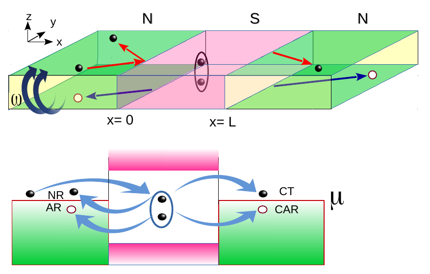
Figure 1: (Color online) Schematic diagram of our geometry and various scattering phenomena, occurring at the thin-topological insulator NSN hybrid structure, is displayed. Light green (light grey) and pink (grey) shadowed regions correspond to the normal (N) and superconducting (S) regions, respectively. Upper panel: Red (black) and blue (black) arrows indicate the direction of electron (black solid bullet) and hole (white hollow bullet), respectively along with the Cooper pair inside the S-region of length $L$. The coupling between the top and bottom surfaces is denoted by $\omega$. Lower panel: Different scattering phenomena in the context of energy band is illustrated considering proximity induced effective pairing gap in S-region. $\mu$ denotes the chemical potential.

junction of thin TI, following Ref. [Majidi and Asgari, 2016], for normal-superconductor (NS) structure. We consider that the entire system lies in the $x$-$y$ plane and a perpendicular electric field is applied along the $z$-direction between the two surfaces via gate electrodes ($U_{top}=U$ and $U_{bottom}=-U$). The middle region of the thin film, as shown by pink shadow in Fig. 1, is the proximity induced superconducting region. The pairing between electron and hole via superconductor can be expressed by the Dirac-Bogoliubov-de Gennes (DBdG) equation as,

$$\left[\begin{array}[c]{c c}\hat{H}(p)-\mu&\hat{\Delta}_{S}\\ -\hat{\Delta}^{\ast}_{S}&\mu-\hat{H}^{\ast}(-p)\\ \end{array}\right]\left[\begin{array}[c]{c}u\\ v\end{array}\right]=\epsilon\left[\begin{array}[c]{c}u\\ v\end{array}\right].$$ (1)

Here, $\mu$ is the chemical potential and $\Delta_{S}$ is the proximity induced superconducting pair potential. The effective single particle Hamiltonian of the thin topological insulator  Zyuzin et al. (2011); Parhizgar et al. (2015); Pershoguba and Yakovenko (2012) can be written as (see Appendix A for the derivation)

$$\hat{H}(p)=\hat{\tau}_{z}\otimes\hat{h}(p)+\hat{\tau}_{x}\otimes\omega\hat{\sigma}_{0}+U\hat{\tau}_{z}\otimes\hat{\sigma}_{0}\ ,$$ (2)

which acts on four component eigen states $\Psi=[\psi_{\it t}^{{\uparrow}},\psi_{\it t}^{{\downarrow}},\psi_{\it b}^{{\uparrow}},\psi_{\it b}^{{\downarrow}}]^{T}$. Here $\omega$ is the coupling between the top and bottom surface states. The energy of the incident electron is denoted by ${\epsilon}$. The pairing symmetry inside the superconducting region is considered to be inter-surface $s$-wave as used in Ref. [Majidi and Asgari, 2016]. It is given by $\hat{\Delta}_{S}=i\Delta_{S}\hat{\sigma}_{y}[\Theta(x-L)-\Theta(x)]$ where $\Theta$ is the Heaviside step function. In the low energy regime, we can write

$$\hat{h}(p)=v_{F}(\hat{\sigma}\times\hat{p})_{z}$$ (3)

with ${\bf p}=\{p_{x},p_{y}\}$ being the $2$D momentum operator and $v_{F}$ denoting the Fermi velocity. We consider here the low energy approximation of $\hat{h}(p)$. With the reduction of thickness of TI, the strength of the coupling between top and bottom surface states ($\omega$) is enhanced. The two sets of Pauli matrices i.e., $\hat{\sigma}$ and $\hat{\tau}$ act on real spin and surface pseudo spin degree of freedom. The energy spectrum in the normal region is given by

$${\epsilon}_{\lambda}^{\pm}(k)=\lambda\sqrt{(\hbar v_{F}|k|\pm U)^{2}+\omega^{2}}-\mu_{N}\ .$$ (4)

where $\lambda=\pm$ denotes band index and $\mu_{N}$ is the chemical potential in the normal region. The coupling parameter $\omega$ controls the band gap between the two surface bands. On the other hand, it is the gate voltage ($U$) which causes energy splitting in the same band.

Similarly inside the superconducting region, characterized by chemical potential $\mu_{S}$, energy dispersion is given by

$${\epsilon}^{\pm}(k_{S})=\sqrt{\mu_{S}-\sqrt{(\hbar v_{F}|k_{S}|\mp U)^{2}+\omega^{2}}+\Delta_{S}^{2}}\ .$$ (5)

The incident electron can undergo four possible scattering events. It can either be normally reflected as an electron via normal reflection (NR), Andreev reflected as a hole with opposite spin, or be transmitted as an electron via CT and as a hole with opposite spin via CAR. These four scattering processes are schematically displayed in the lower panel of Fig. 1. Note that, unlike graphene where Andreev phenomenon occurs between two valleys, here each conducting surface contains single Dirac cone. Hence Andreev phenomenon occurs between the two surfaces (top and bottom) due to the inter-surface pairing symmetry as assumed in our analysis. If the incident electron belongs to the top surface, then the reflected or transmitted hole via the AR and CAR respectively take place in the bottom surface. On the other hand, NR and CT correspond to the top surface as shown in the upper panel of Fig. 1.

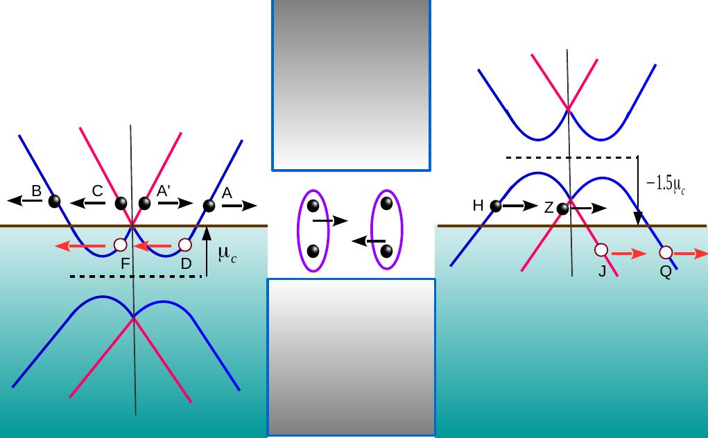
Figure 2: (Color online) Schematic diagram of different scattering processes for the chemical potential $\mu_{L}=\mu_{c}$ and $\mu_{R}=-1.5\mu_{L}$ is depicted. The left and right regions are the normal thin TI while the middle one is the proximity induced superconducting region following the energy dispersion as given in Eqs.(4)-(5). Electrons and holes are denoted by black bullets and empty white bubbles, respectively. The horizontal black arrows indicate the direction of propagation of electrons while, the red (light grey) ones are used for the holes, respectively. Two energy branches ${\epsilon}_{\lambda}^{+}$ and ${\epsilon}_{\lambda}^{-}$ are indicated by red (grey) and blue (grey) curves, respectively.

III Numerical results

In this section we present our numerical results for the scattering amplitudes, conductance and shot-noise in three different sub-sections. We discuss our results in terms of the scattering processes occurring at the interface of the hybrid structure and various parameters of the system.

III.1 Scattering amplitudes

In order to discuss the results for the scattering amplitudes, we consider two different situations by setting the chemical potential in the right normal thin TI region at two different doping levels ($p$-type). They are at $\mu_{R}=-1.5\mu_{L}$ and $\mu_{R}=-\mu_{L}$ respectively while the chemical potential $\mu_{L}$ at the left normal thin TI region is fixed to $\mu_{c}$ ($n$-type). Here, $\mu_{c}=\sqrt{U^{2}+\omega^{2}}$ is the critical chemical potential at which energy branches cross each other at zero momentum. The superconductor is doped at $\mu_{S}=1$ eV. We choose $\mu_{S}\gg\Delta_{S}$ for the requirement of the mean-field treatment of superconductivity Beenakker (2006, 2008).

III.1.1 Case I : $\mu_{{}_{R}}=-1.5\mu_{{}_{L}}$

In Fig. 2 we show a schematic diagram for the different scattering channels. The gate voltage induced energy splitting in the same band opens up two different incident channels ($A$ and $A^{\prime}$) for an electron with the same energy but with different momentum. An electron with incoming energy $\epsilon>0$, incident from $A$ or $A^{\prime}$, can either be reflected or transmitted as an electron or hole through a pair of reflection and transmission channels. The normal reflection as electron can happen through $B$ and $C$ whereas the possible Andreev reflection channels are $D$ and $F$ respectively. On the other hand, transmission either as an electron via CT or as a hole via CAR can take place via $Z$ and $H$ or $J$ and $Q$, respectively, as demonstrated in Fig. 2. The Andreev reflection corresponding to $D$ channel is retro type while it is specular for the channel $F$ Majidi and Asgari (2016). Most remarkably, this specular AR is intra-band which is in complete contrast to graphene where inter-band specular AR was predicted by Beenakker Beenakker (2006). However, in thin TI, CT and CAR can be either intra-branch or inter-branch type originating from the same band.

To obtain the different scattering amplitudes, we match the wave functions across the boundary at $x=0$ and $x=L$ (see Fig. 1), i.e., $\Psi_{L}|_{x=0}=\Psi_{S}|_{x=0}$ and $\Psi_{S}|_{x=L}=\Psi_{R}|_{x=L}$ where $\Psi_{L(R)}$ and $\Psi_{S}$ are the wave functions corresponding to the left (right) normal region and superconducting region, respectively (see Appendix B for the explicit form of the wave functions). For an incoming electron from $j=\{A,A^{\prime}\}$, we denote the CT and CAR amplitudes by $t_{Z}^{e}$, $t_{H}^{e}$ and $t_{Q}^{h}$, $t_{J}^{h}$ corresponding to the channels $Z$, $H$, $Q$ and $J$, respectively. On the other hand, NR and AR amplitudes are denoted by $r_{B}^{e}$, $r_{C}^{e}$ and $r_{D}^{h}$, $r_{F}^{h}$ for the channels $B$, $C$, $D$, and $F$ respectively. The superscript ‘$e$’ and ‘$h$’ denote electron and hole, respectively. Note that, for both the incoming channels ($A$ and $A^{\prime}$) scattering probabilities satisfy unitarity condition. It can be expressed as

$$\sum_{\iota}R_{\iota}^{e}+\sum_{\eta}R_{\eta}^{h}+\sum_{\bar{\iota}}T_{\bar{\iota}}^{e}+\sum_{\bar{\eta}}T_{\bar{\eta}}^{h}=1\ .$$ (6)

where $R_{\iota}^{e}=|r_{\iota}^{e}|^{2}$ with $\iota=\{B,C\}$, $R_{\eta}^{h}=|r_{\eta}^{h}|^{2}$ with $\eta=\{F,D\}$, $T_{\bar{\iota}}^{e}=|t_{\bar{\iota}}^{e}|^{2}$ with ${\bar{\iota}}=\{Z,H\}$ and $T_{\bar{\eta}}^{h}=|t_{\bar{\eta}}^{h}|^{2}$ with ${\bar{\eta}}=\{J,Q\}$. The wave vectors for different transmission channels are given by $|k_{Z(H)}|=[\sqrt{({\epsilon}+\mu_{R})^{2}-\omega^{2}}\mp U]/(\hbar v_{F})$ and $|k_{J(Q)}|=[\sqrt{({\epsilon}-\mu_{R})^{2}-\omega^{2}}\mp U]/(\hbar v_{F})$.

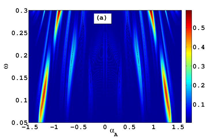
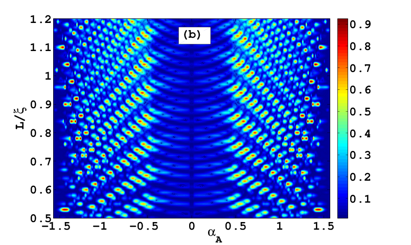
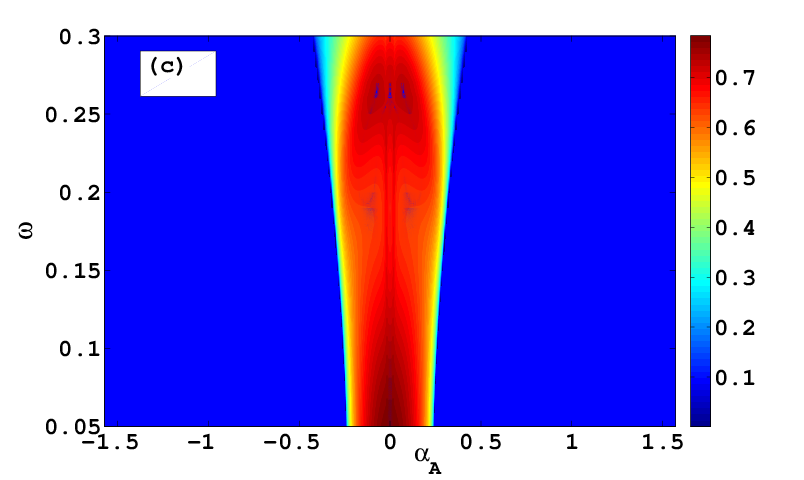
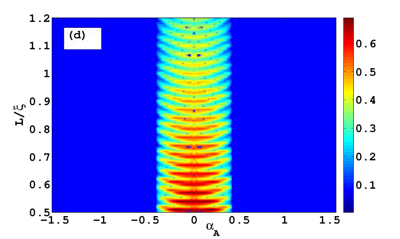
Figure 3: (Color online) The behavior of CAR probability at $Q$ i.e., $T_{Q}^{h}$ is illustrated in panel (a) $\omega$$-$$\alpha_{A}$ plane and panel (b) $L/\xi$ $-$ $\alpha_{A}$ plane for an incident electron at $A$. Similarly, CT probability at $Z$ ($T_{Z}^{e}$) is shown in panel (c) and (d) in the same parameter space. The value of the other parameters are chosen to be gate potential $U=0.3$ eV, excitation energy ${\epsilon}/\Delta_{S}=1$. We choose $L/\xi=0.5$ for the left column and $\omega=0.3$ eV for the right column.

For the above-mentioned scenario, we discuss the features of CT and CAR probabilities as a function of the coupling strength $\omega$, angle of incidence $\alpha_{A}$ and the length $L$ of the superconducting region. We set the energy of the incident electron as ${\epsilon}/\Delta_{S}=1$. In Ref. [Majidi and Asgari, 2016] it is already been explored that specular AR can occur with $100\%$ efficiency for a wide range of angle of incidence at this energy. Hence, we also choose this particular energy value for our investigation of CAR. In the left column of Fig. 3, we show the behavior of CAR and CT probability in the $\omega$$-$$\alpha_{A}$ plane, while in the right column the same has been depicted in the $L/\xi$$-$$\alpha_{A}$ plane, for an incoming electron from channel $A$. From Fig. 3(a), we observe that CAR probability at $Q$ ($T_{Q}^{h}$) exhibits a maxima for a particular angle of incidence $\alpha_{A}$ and coupling constant $\omega$. $T_{Q}^{h}$ can reach around $50\%$ probability for the set of parameter values like $\alpha_{A}\simeq\pm 0.95$ and $\omega=0.3$ eV as well as $\alpha_{A}=\pm 1.3$ and $\omega\sim 0.1$ eV. Note that, this CAR process is inter-band but intra-branch type with the incident electron and transmitted hole energy as ${\epsilon}^{-}_{+}$ and ${\epsilon}^{-}_{-}$, respectively. This feature is shown for $L/\xi=0.5$. In Fig. 3(b), we investigate the behavior of CAR as a function of the length of the superconducting region $L/\xi$ and find that it exhibits a rib-like pattern characterized by several resonances with the variation of both the length of the superconducting region and angle of incidence $\alpha_{A}$. Note that, in the $L/\xi$$-$$\alpha_{A}$ plane, CAR can be achieved even with $90\%$ probability under suitable circumstances. However, it is found to be absent for normal incidence ($\alpha_{A}=0$) as in this case all the electrons are locally reflected as holes due to AR.

On the other hand, CT manifests a completely different behavior with the variation of the length of S-region as well as the angle of incidence.

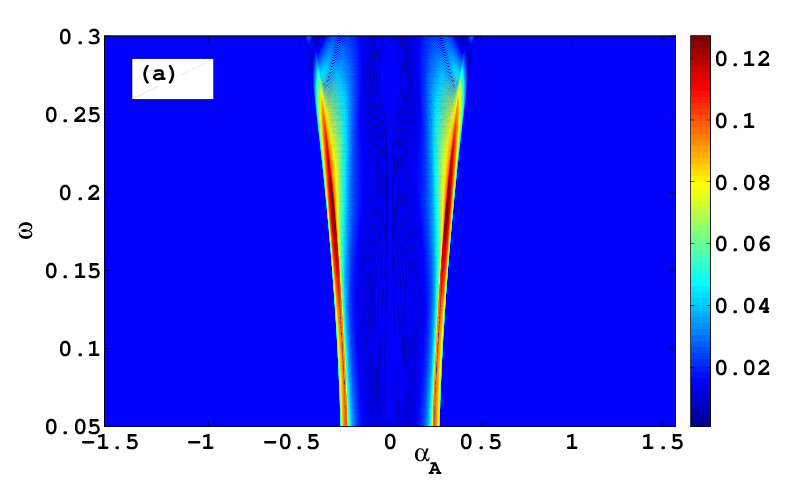
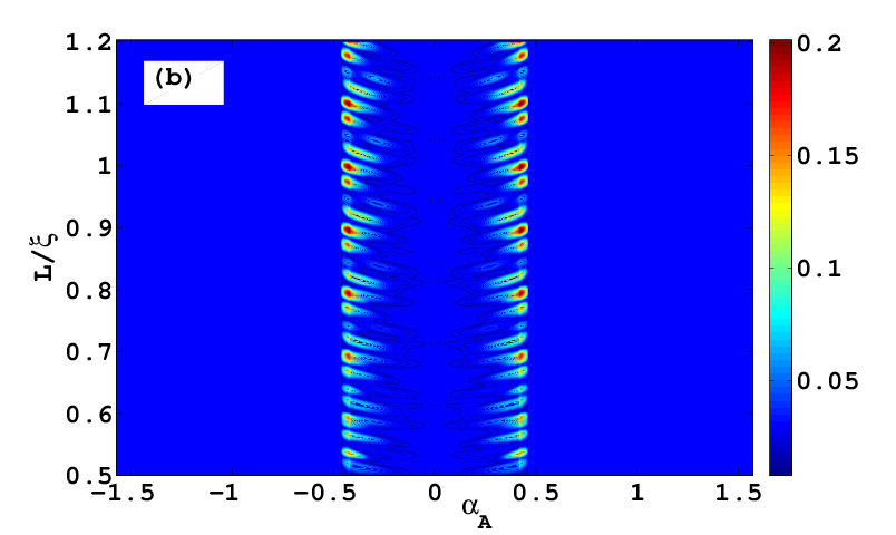
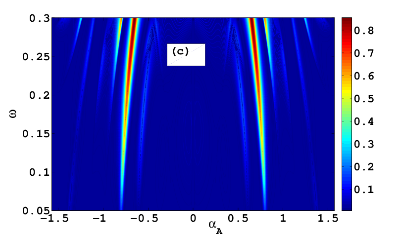
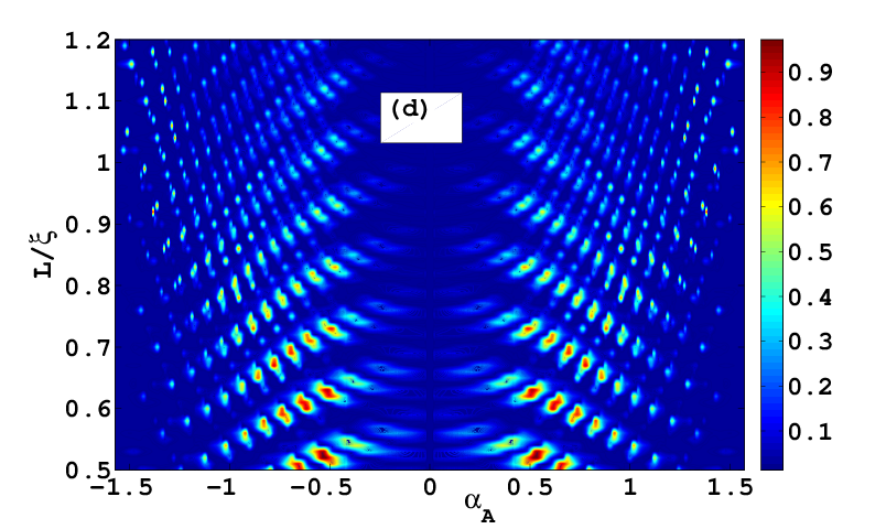
Figure 4: (Color online) The behavior of CAR probability at $J$ i.e., $T_{J}^{h}$ is shown in panel (a) and (b) in the $\omega$ $-$ $\alpha_{A}$ and $L/\xi$ $-$ $\alpha_{A}$ plane, respectively. Similarly, the behavior of CT probability at $H$ ($T_{H}^{e}$) in the plane of $(\omega,\alpha_{A})$ and ($L/\xi,\alpha_{A}$) are portrayed in panel (c) and (d), respectively. The value of the other parameters are chosen to be the same as mentioned in Fig. 3.

In Fig. 3(c), we observe that the probability of CT at $Z$ i.e., $T_{Z}^{e}$ exhibits a continuous band-like profile around an angular region, confined by the critical angle $\alpha_{A}^{c}$, as one increases the coupling strength $\omega$ between the two surfaces. Most interestingly, maxima of $T_{Z}^{e}$ appears even for relatively weak coupling strength in contrast to CAR at $Q$ as it’s an intra-band process. Although $T_{Z}^{e}$ is inter-branch type as incident and transmitted electrons are from ${\epsilon}_{+}^{-}$ and ${\epsilon}_{-}^{+}$, respectively. It can be explained as Klein tunneling phenomena as $T_{Z}^{e}=1$ at $\alpha_{A}=0$, being almost independent of the coupling strength. When we change the length of the superconducting region, the behavior of CT manifests an oscillatory pattern as displayed in Fig. 3(d). It mimicks a spinal-chord like pattern with a linearly decaying amplitude with the enhancement of the superconducting length within the range confined by $-\alpha_{A}^{c}$ to $\alpha_{A}^{c}$. It is apparent from Fig. 3(c)-(d) that the CT phenomena at $Z$ is limited by the critical angle in contrast to the CAR at $Q$ channel.

In Fig. 4, we discuss the behavior of CAR and CT probabilities for other transmission channels, i.e., CAR at $J$ and CT at $H$ (see Fig. 2). In Fig. 4(a) we show the features of $T^{h}_{J}$ in the $\omega$$-$$\alpha_{A}$ plane for a fixed value of $L$ ($=0.5\xi$). Throughout the contour CAR probability is vanishingly small except for a very narrow region on both sides of

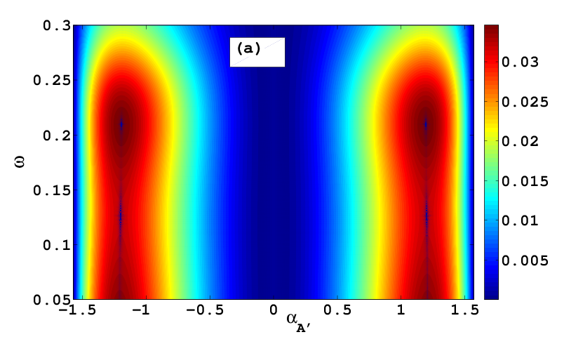
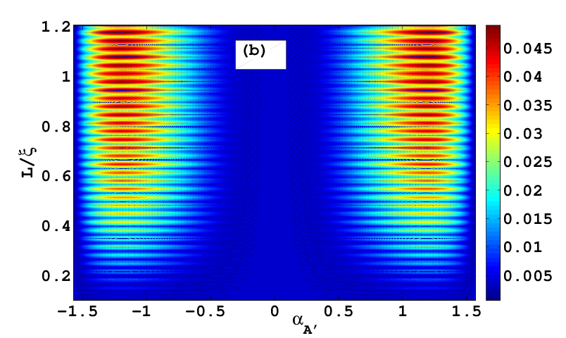
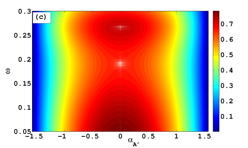
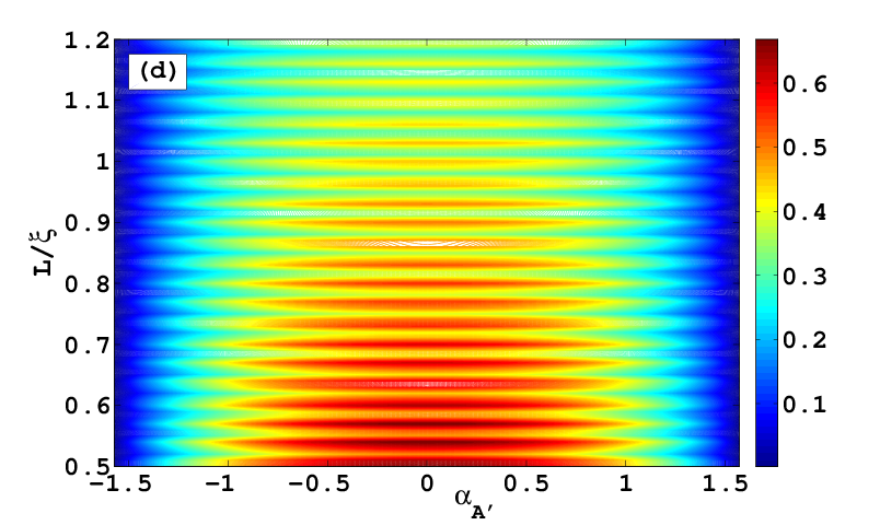
Figure 5: (Color online) The variation of CAR probability at $Q$, $T_{Q}^{h}$, is demonstrated in panel (a) and (b) in the plane of $(\omega,\alpha_{A^{\prime}})$ and $(L/\xi,\alpha_{A^{\prime}})$, respectively. Whereas, the behavior of CT probability at $Z$, $T_{Z}^{e}$ is shown in the plane of $(\omega,\alpha_{A^{\prime}})$ and ($L/\xi,\alpha_{A^{\prime}}$) in panel (c) and (d), respectively. Here the incident electron is considered via $A^{\prime}$ channel (see Fig. 2). We choose the same values of the other parameters as mentioned in Fig. 3.

$\alpha_{A}=0$. The maximum probability of CAR via channel $J$, which arises for a regime of coupling $\omega\sim 0.15-0.25$, is of the order of $12\%$. This is smaller in magnitude compared to the CAR obtained via channel $Q$. Such difference between the probabilities of CAR via the two channels can be explained as follows. For the electron incident from the channel $A$, change of energy branch associated with a momentum transfer, is required in order to obtain CAR at $J$. Whereas it is intra-branch process for $Q$. However, as one increases the length of the superconducting region, reduction or enhancement in CAR takes place at $J$ depending on the value of $\omega$ and $\alpha_{A}$. By varying the length of the superconducting region, we can achieve CAR with maximum $20\%$ probability being confined by the same angular space defined by the critical angle $\alpha_{A}^{c}$, as shown in Fig. 4(b). The latter manifests a spinal chord-like pattern, in the behavior of CAR probability, with the variation of $L/\xi$ and $\alpha_{A}$.

On the other hand, the CT at $H$ ($T^{e}_{H}$) exhibits intriguing features as depicted in Fig. 4(c)-(d). The behavior of CT is not limited by the critical angle as before. In Fig. 4(c) we show the behavior of $T^{e}_{H}$ in the $\omega$ $-$ $\alpha_{A}$ plane for $L/\xi=0.5$. Here, $T^{e}_{H}$ with maximum probability around $85\%$ can be obtained within a very narrow region at a particular angle of incidence $\alpha_{A}$. Moreover, it increases with the strength of the coupling between the two surfaces of TI. However, the pattern changes to rib-like while we investigate CT at $H$, in the plane spanned by $L/\xi$ and $\alpha_{A}$ as shown in Fig. 4(d). Also, it becomes oscillatory with decaying magnitude with the enhancement of the length of the superconductor for a fixed value of $\omega$ and $\alpha_{A}$. This feature is evident from Fig. 4(d). Similar behavior is obtained for some other values of $\alpha_{A}$ also. The decaying nature of CT is also obtained when we vary $\alpha_{A}$ for a particular value of $L/\xi$. Here, CT at normal incidence is found to be absent. Interestingly, more than $80\%$ inter-branch CT at $Z$ can be obtained for a wide range of angle of incidence while intra-branch CT at $H$ appears at a particular angle of incidence $\alpha_{A}$.

As mentioned earlier, for a particular energy there are two channels corresponding to two different momenta available for the electron to be incident on the NS interface. Here, we present our discussion of CAR and CT probabilities for an incoming electron incident from $A^{\prime}$. In Fig. 5(a)-(b), we demonstrate the behavior of $T^{h}_{Q}$ in the plane of ($\omega$, $\alpha_{A^{\prime}}$) and ($L/\xi$, $\alpha_{A^{\prime}}$) respectively. Similarly, Fig. 5(c)-(d) illustrate the variation of $T^{e}_{Z}$ in $\omega$$-$$\alpha_{A^{\prime}}$ and $L/\xi$$-$$\alpha_{A^{\prime}}$ plane respectively. From Fig. 5(a) we observe that the probability for CAR at $Q$ is vanishingly small for all values of coupling constant and angle of incidence from channel $A^{\prime}$. The maximum CAR probability, that we can achieve in this case, is about $3\%$ which is significantly smaller in magnitude compared to that of the same for channel $A$. This reduction appears due to the momentum difference between $A$ and $A^{\prime}$. This behavior is also almost independent of $\omega$. We present our result for $\omega=0.05-0.3$ eV which covers the experimentally achievable value Zhang et al. (2010). Although this phenomenon is true for a particular value of $L/\xi$, the result does not change by appreciable amount when we change the length of the superconducting region. In Fig. 5(b), we show the corresponding behavior of CAR in $L/\xi$$-$$\alpha_{A^{\prime}}$ plane. On the other hand, in contrast to CAR, CT is the dominating process for a wide range of $\omega$. This is evident from Fig. 5(c). Also note that, CT at normal incidence can dominate over the other scattering processes even for weakly coupled surface states as shown in Fig. 5(c). However, such behavior is not entirely independent of the coupling constant. Apart from the weak coupling limit, a resonance can also be obtained at around $\omega=0.26$ eV. To reveal the behavior of CT at $Z$, as a function of the superconducting length, we present Fig. 5(d) where it is shown that the probability of CT at $Z$ manifests an oscillatory behavior. Although the amplitude of oscillation decreases as we

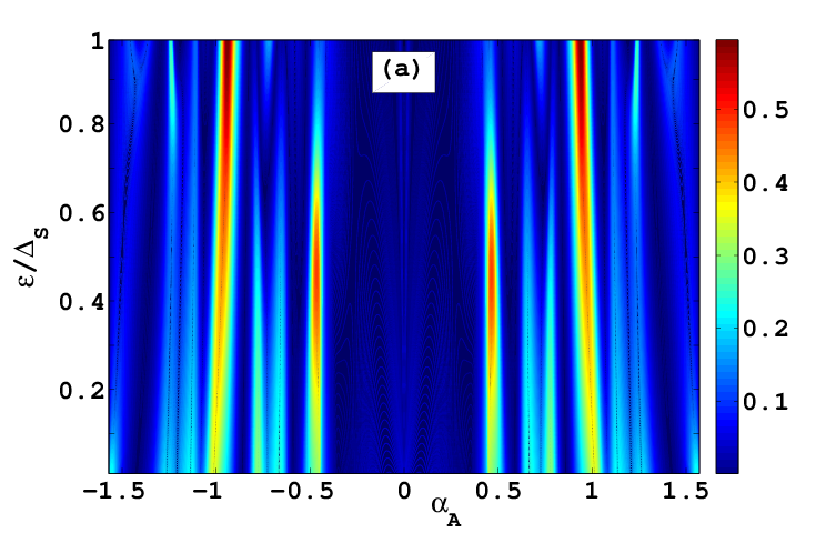
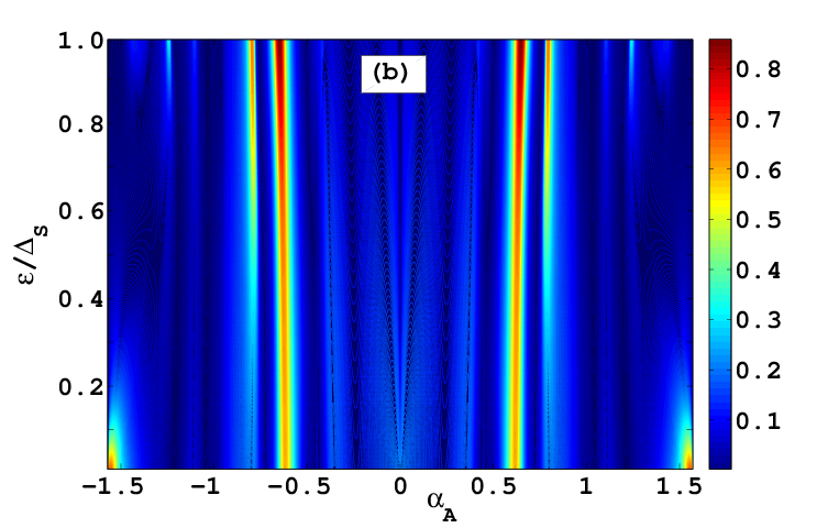
Figure 6: (Color online) The variation of CAR at $Q$ and CT probability at $Z$, in the $\epsilon/\Delta_{s}$$-$$\alpha_{A}$ plane, is illustrated in panel (a) and (b) respectively . The length of superconducting region is considered to be $L=0.5\xi$. The value of the other parameters are chosen to be $\omega=0.3$ eV and $U=0.3$ eV.

increase the length of the superconductor, even for normal incidence. Here we present our result for $\omega=0.3$ eV for which we can achieve the maximum value of CT probability $\sim 0.6$. The oscillatory response of CAR and CT with the enhancement of the superconducting length is similar to the previous case (see Fig. 3). Nevertheless, the difference lies in the fact that in Fig. 5(d) the angular region, spanned by the angle of incidence for CT, is wider compared to that of depicted in Fig. 3(d).

Similar to the case of incident channel at $A$, we can have CAR and CT probabilities at $J$ and $H$ also for the incident channel at $A^{\prime}$. Although they appear to be very small in magnitude for all values of $\omega$ and $L/\xi$. Hence, we do not show those results explicitly. The reason for vanishingly small CAR and CT probabilities for an incident electron from $A^{\prime}$ can be attributed to the small $x$-component of momentum in comparison to $A$.

Finally, we look into the behavior of CAR and CT probabilities with the variation of both incident electron (from point $A$) energy, below the subgapped regime, and incident angle ($\epsilon/\Delta_{s}$$-$$\alpha_{A}$ plane) as shown in Fig. 6. It is observed that CAR probability at $Q$ ($T^{h}_{Q}$) at a certain angle of incidence attains maximum value when energy of the incident electron becomes nearly equal to the proximity induced superconducting gap i.e., ${\epsilon}\simeq\Delta_{S}$ (see Fig. 6(a)). On the oher hand, CT probability at $Z$ ($T^{e}_{Z}$) also exhibits similar behavior like CAR, as depicted in Fig. 6(b). The behavior of CAR and CT for the $A^{\prime}$ channel is also very similar to that of $A$ channel.

III.1.2 Case II: $\mu_{R}=-\mu_{L}$

In this subsection, we discuss the scenario where the chemical potential in the $p$-type normal region is lifted to $\mu_{{}_{R}}=-\mu_{{}_{L}}=-\mu_{c}$. For this case, all possible scattering channels are shown in Fig. 7. Note that, now two CT channels belong to the same branch associated with a sign change in the $x$-component of momentum in one CT channel at $R$, i.e., from $-k_{Z}^{x}\rightarrow k_{R}^{x}$.

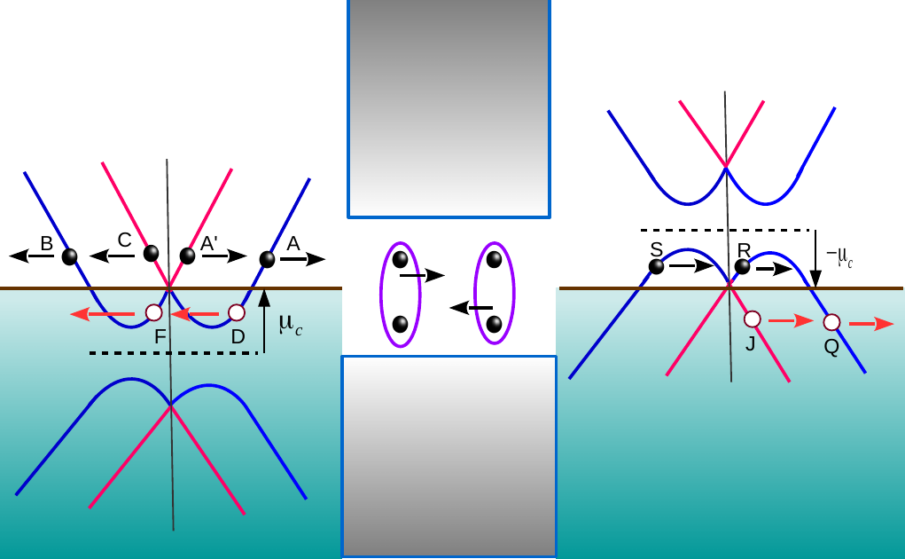
Figure 7: (Color online) Schematic diagram of different scattering channels for our NSN hybrid structure when $\mu_{R}=-\mu_{L}$. We adopt the same convention, mentioned in Fig. 2, to denote electrons and holes and their propagation direction.

The group velocity of the electron, along the $x$-direction, corresponding to the transmission channels at $R$ and $S$ would be positive as long as the slope $\partial E/\partial k_{x}>0$. This corresponds to the fact that group velocity along the $x$-direction can be positive even for negative $x$-component of momentum. Following the previous case, we also analyze here the behavior of CT and CAR probabilities, for an electron incoming from $A$.

In Fig. 8(a), we show the behavior of CAR probability at $Q$ as a function of the coupling strength ($\omega$) and angle of incidence ($\alpha_{A}$) considering the same length of the superconductor as mentioned in the previous cases. The most interesting feature is that CAR probability can be enhanced to more than $95\%$ in the $\omega$$-$$\alpha_{A}$ plane. This enhancement may be related to the matching of the $x$-component of the wave vector of the incident electron at $A$ with that of transmitted hole at $Q$. In particular, this feature appears for $\omega=0.16$ eV at a particular angle of incidence away from $\alpha_{A}=0$. On the other hand, CT at $R$ is allowed only through a very narrow angular region around $\alpha_{A}=0$ as shown in Fig. 8(c). The behavior of CAR and CT with the variation of the length of the superconducting region is illustrated in Figs. 8(b) and (d), respectively. The corresponding behavior of CAR probability at $Q$ preserves the rib-like pattern in the $L/\xi$$-$$\alpha_{A}$ plane as before (see Fig. 8(b)). Moreover, CT takes place with finite probability only around the normal incidence and decays with the enhancement of the length of the superconducting region as depicted in Fig. 8(d). Note that, CAR at $J$ is very small compared to $Q$. Also CT at $S$ exhibits similar behavior as of $H$ in the previous case. The contribution arising from incident electron at $A^{\prime}$ is also too small compared to that of $A$.

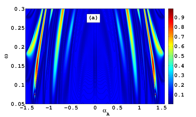
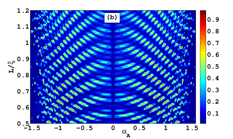
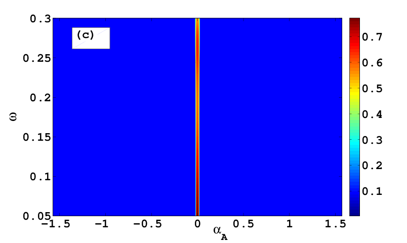
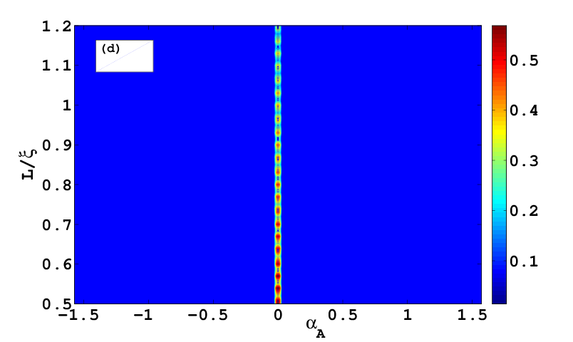
Figure 8: (Color online) The behavior of CAR probability at $Q$ i.e., $T_{Q}^{h}$ is shown in panel (a) and (b) in the plane of $(\omega,\alpha_{A})$ and $(L/\xi,\alpha_{A})$, respectively. Similarly, CT probability at $R$ i.e., $T_{R}^{e}$ is demonstrated in the same parameter space in panel (c) and (d), respectively. The incident electron is considered to be from $A$. We choose the same values of the other parameters as mentioned in Fig. 3.

Therefore, by adjusting the chemical potential or the doping concentration in the right normal region from $\mu_{{}_{R}}=-1.5\mu_{c}$ to $-\mu_{c}$, CAR probability can be maximally enhanced to $97\%$ even for finite angle of incidence (see Fig. 8(a)). This is the key result of our paper. The striking feature is, unlike graphene, in thin TI hybrid junction a large CAR can be achieved even when both the normal regions are sufficiently doped. One can achieve CAR with $100\%$ probability in graphene NSN junction under very special circumstances where the chemical potential in the $p$-doped region is chosen in such a way that CT channel falls exactly at the band touching point for which electron does not possess non-zero momentum, and hence only CAR mechanism is possible Cayssol (2008). In massive Dirac material like silicene, chemical potential has to be adjusted at the bottom and top of the conduction (left region) and valence (right region) band, respectively, so that energy band cannot support AR and CT due to the mass gap. As a result, the incident electron can either be normally reflected or transmitted as a hole via the CAR process Linder and Yokoyama (2014); Paul and Saha (2017). Moreover, in silicene, this phenomena only occurs at normal incidence of electron i.e., $\alpha_{A}=0$. In this context, our system can be more advantageous in order to obtain large CAR probability without concomitant CT, but with finite doping and oblique incidence.

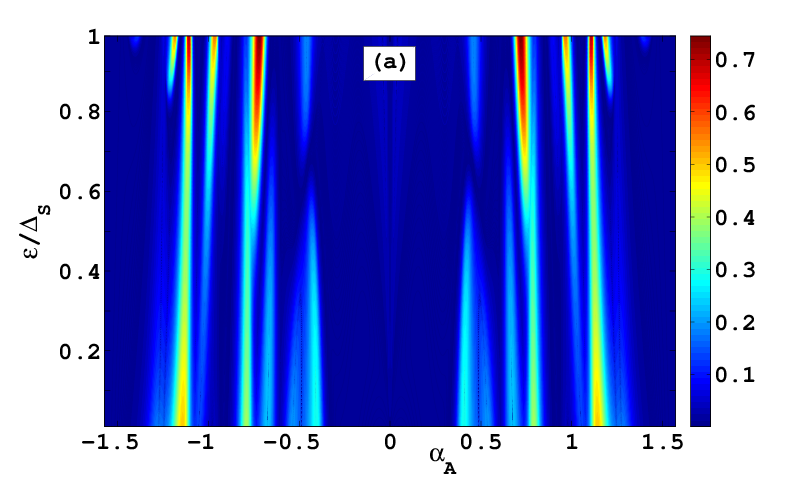
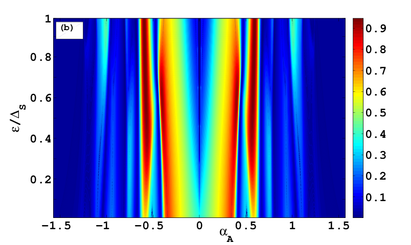
Figure 9: (Color online) The features of CAR at $Q$ and CT probability at $R$, in ${\epsilon}/\Delta_{S}$$-$$\alpha_{A}$ plane, are displayed in panel (a) and (b) respectively. The value of the other parameters are chosen to be the same as mentioned in Fig. 6.

In Fig. 9, we investigate the variation of CAR at $Q$ ($T^{h}_{Q}$) and CT probabilities at $R$ ($T^{e}_{R}$) in the ${\epsilon}/\Delta_{S}$$-$$\alpha_{A}$ parameter space. Note that, CAR probability attains a maximum for ${\epsilon}\sim\Delta_{S}$ for a certain angle of incidence. This feature is depicted in Fig. 9(a). Also this is very similar to the previous case (see Fig. 6(a)). On the contrary, CT at $R$ can be quite high ($\sim 90\%$) for a wide range of incident electron energy ${\epsilon}$ at a particular angle of incidence. This is shown in Fig. 9(b). For the other incoming channel $A^{\prime}$, we have checked that both electron and hole transmissions are vanishingly small in the same parameter regime.

III.2 Conductance

In this subsection, we investigate the angle-averaged normalized differential conductance for the two cases representing two different chemical potentials (doping concentration) in the right normal region. We employ extended BTK formalism Blonder et al. (1982); Beenakker (2006) to compute our conductance. The differential conductance corresponding to the elastic CT of electron at a particular angle of incidence ($\alpha_{j}$), where $j$ may be $A$ or $A^{\prime}$, via transmission channel $\eta$ can be expressed as

$$G_{\rm CT}=\frac{e^{2}}{h}\sum_{j}\sum_{\eta}|t_{\eta}^{e}(\alpha_{j})|^{2}.$$ (7)

The transmission channel $\eta$ can be $\{Z,H\}$ or $\{R,S\}$ depending on the doping level either at $\mu_{{}_{R}}=-1.5\mu_{{}_{L}}$ or at $\mu_{{}_{R}}=-\mu_{{}_{L}}$, respectively.

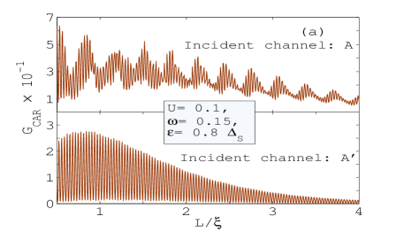
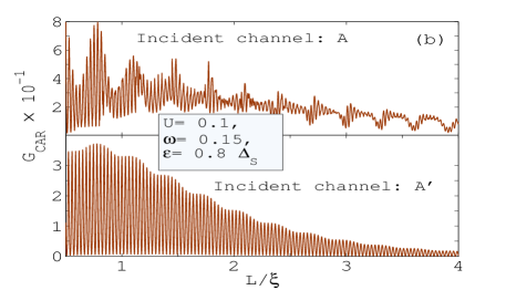
Figure 10: (Color online) The behavior of angle averaged differential CAR conductance, in units of $G_{0}$, is shown as a function of the length of the superconductor. Here, $\omega$ and $U$ are in units of $\rm eV$. Panel (a) and (b) correspond to the case $\mu_{R}=-1.5\mu_{L}$ and $\mu_{R}=-\mu_{L}$ respectively.

After averaging over the angle of incidence the conductance reduces to

$$\frac{G_{\rm CT}}{G_{0}}=\sum_{j}\int_{-\pi/2}^{\pi/2}\sum_{\eta}|t_{\eta}^{e}(\alpha_{j})|^{2}\cos\alpha_{j}d\alpha_{j}\ ,$$ (8)

where $G_{0}=(e^{2}/h)N$, $N=kW/\pi$ being the number of transverse modes and $W$ is the width of the thin TI. Similar expression can be used for the CAR conductance as well

$$\frac{G_{\rm CAR}}{G_{0}}=\sum_{j}\int_{-\pi/2}^{\pi/2}\sum_{\bar{\eta}}|t_{\bar{\eta}}^{h}(\alpha_{j})|^{2}\cos\alpha_{j}d\alpha_{j}\ .$$ (9)

where $\bar{\eta}$ can be $\{Q,J\}$. Finally we compute the total two terminal differential conductance by using the relation

$$\frac{\partial I}{\partial V}=G=\frac{G_{\rm CT}-G_{\rm CAR}}{G_{0}}\ .$$ (10)

In Fig. 10, we illustrate the behavior of angle averaged CAR conductance for an incoming electron from $A$ (upper row of Fig. 10(a)-(b)) and $A^{\prime}$ (bottom row of Fig. 10(a)-(b)) with the variation of the length of the superconductor. Here we also investigate how the thickness induced coupling parameter $\omega$ and the doping level $\mu_{R}$ in the right normal region affect the CAR conductance. We find that, when $\mu_{R}=-1.5\mu_{L}$, CAR conductance exhibits an oscillatory behavior as we vary $L/\xi$ (see Fig. 10(a)). This result is consistent with the previous oscillatory nature of CAR probability. Such oscillatory nature of CAR conductance can be a direct manifestation of closely spaced Andreev bound state levels inside the superconducting region. Moreover, change of incoming channel seems to induce an additional oscillation envelope due to the coupling between the two TI surfaces, as depicted in the upper row of Fig. 10(a). Such oscillation in CAR conductance can be observed when the electron is incident via channel $A$. However, this additional oscillation is not visible for the incident electron at $A^{\prime}$ (see lower row of Fig. 10(a)). For $\mu_{R}=-\mu_{L}$ the behavior as well as the magnitude of the oscillation appears to be similar as $\mu_{R}=-1.5\mu_{L}$ case (see Fig. 10(b)). Note that, similar oscillatory behavior of the angle averaged CT conductance also exists.

In Fig. 11, we show the behavior of angle averaged differential conductance $G$ (in unit of $G_{0}$) as a function of the incident electron energy $\epsilon$ in the subgapped regime ($\epsilon\leq\Delta_{s}$) incorporating contributions arising from both the incident channels $A$ and $A^{\prime}$. Here, the doping level in the right normal region is $\mu_{R}=-1.5\mu_{L}$. From Figs. 11(a)-(b), it is apparent that CAR can dominate over CT within the regime ${\epsilon}\leq 0.8\Delta_{s}$. However, this phenomenon is very sensitive to the coupling $\omega$ as well as the length of the superconducting region $L$. In fact, a smooth variation of $\omega$ can reduce the CT conductance resulting in higher CAR contribution which can be observed in Fig. 11(b). The competition between these two scattering processes give rise to positive or negative values of relative $G$. The results are of same nature for $\mu_{R}=-\mu_{L}$ case which is shown in Figs. 11(c)-(d). It can be seen that the coupling between the two TI surfaces enhances CAR conductivity by a larger amount compared to that of $\mu_{R}=-1.5\mu_{L}$. Therefore, in our NSN hybrid structure, CAR conductance can dominate over the CT conductance, below the subgapped regime, under suitable circumstances.

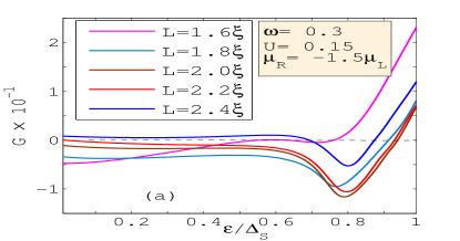
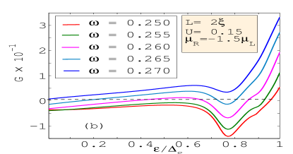
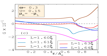
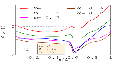
Figure 11: (Color online) The behavior of angle averaged differential conductance $G=G_{CT}-G_{CAR}$, in units of $G_{0}$, is demonstrated as a function of $\epsilon/\Delta_{S}$ in the subgapped regime. Here, $\omega$ and $U$ are in the units of $\rm eV$.

III.3 Shot noise

This subsection is devoted to the analysis of zero-frequency shot noise cross correlation for our hybrid NSN model following Refs.[Blanter and Büttiker, 2000; Anantram and Datta, 1996]. The current-current correlation function between the two leads, labeled by $i$ and $j$, is given by

$$S_{ij}(t-t^{\prime})={\langle}\Delta\hat{I}_{i}(t)\Delta\hat{I}_{j}(t^{\prime})+\Delta\hat{I}_{j}(t^{\prime})\Delta\hat{I}_{i}(t){\rangle}\ ,$$ (11)

where the current fluctuation operator is defined as

$$\Delta\hat{I}_{i}(t)=\hat{I}_{i}(t)-{\langle}\hat{I}_{i}(t){\rangle}\ .$$ (12)

The correlation function defined in Eq.(11) can be transformed in Fourier space as

$$S_{ij}(\Omega)\delta(\Omega+\Omega^{\prime})=\frac{1}{2\pi}{\langle}\Delta\hat{I}_{i}(\Omega)\Delta\hat{I}_{j}(\Omega^{\prime})+\Delta\hat{I}_{j}(\Omega^{\prime})\Delta\hat{I}_{i}(\Omega){\rangle}\ ,$$ (13)

with

$$\Delta\hat{I}_{i}(\Omega)=\hat{I}_{i}(\Omega)-{\langle}\hat{I}_{i}(\Omega){\rangle}\ .$$ (14)

Now using $\int dt~{}e^{({\epsilon}-{\epsilon}^{\prime})t/\hbar}=2\pi\hbar\delta({\epsilon}-{\epsilon}^{\prime})$, the zero frequency shot noise cross-correlation between the two leads, $i$ and $j$, in terms of scattering amplitudes can be generalized in presence of an external bias as Anantram and Datta (1996)

$$S_{ij}({\epsilon}) = \frac{2e^{2}}{h}\sum_{k,l\in N,S;\alpha,\beta,\gamma,\delta\in e,h}sgn(\alpha)sgn(\beta)$$

$$A_{k\gamma,l\delta}(i\alpha,{\epsilon})A_{l\delta,k\gamma}(j\beta,{\epsilon})f_{k\gamma}({\epsilon})[1-f_{l,\delta}({\epsilon})]\ ,$$

where $A_{k\gamma,l\delta}(i\alpha,{\epsilon})=\delta_{ik}\delta_{il}\delta_{\alpha\gamma}\delta_{\alpha\delta}-s_{ik}^{\alpha\gamma^{\dagger}}({\epsilon})s_{il}^{\alpha\delta}({\epsilon})$. Here, $s_{ik}^{\alpha\gamma}$ denotes the scattering amplitude for a $\gamma$ type particle incident from lead $k$ being scattered to lead $i$ as a particle type $\alpha$ ($\alpha,\gamma\in e,h$) where $e$ ($h$) stands for electron (hole). Also $sgn(\alpha)$ ($sgn(\beta)$) can be $+~{}(-)$ corresponding to $e$ ($h$). As the scattering amplitudes are function of angle of incidence, we perform the angle average of shot noise cross-correlation incorporating the contributions arising from both the incoming channels of the incident electron ($A$ and $A^{\prime}$),

$$S_{ij}({\epsilon})=\int_{-\pi/2}^{\pi/2}S_{ij}(\alpha_{A},{\epsilon})d\alpha_{A}+\int_{-\pi/2}^{\pi/2}S_{ij}(\alpha_{A^{\prime}},{\epsilon})d\alpha_{A^{\prime}}\ .$$ (16)

A simplified analytical expression of the zero frequency shot noise cross-correlation that we use for our numerical computation is given in Appendix C.

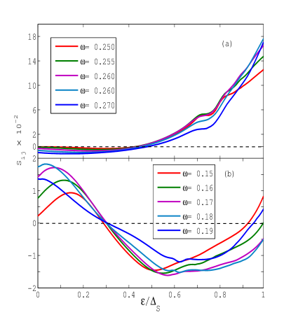
Figure 12: The behavior of shot noise cross correlation $S_{ij}$ (in units of $e^{2}/h$) is illustrated as a function of $\epsilon/\Delta_{S}$ in the subgapped regime. Here panel (a) and (b) correspond to the case (a) $\mu_{R}=-1.5\mu_{L}$ and (b) $\mu_{R}=-\mu_{L}$ respectively and $\omega$ is in the unit of $\rm eV$. The value of the other parameters are $U=0.1$ eV and $L=2\xi$.

In Fig. 12 we show the features of the shot noise cross-correlation $S_{ij}$ with the variation of the incoming electron energy $\epsilon$ below the subgapped regime ($\epsilon\leq\Delta_{S}$). We observe that shot noise changes sign from negative to positive depending on the incoming electron energy as well as the coupling $\omega$ between the two TI surfaces. When the chemical potential in the right normal region is set to the value $\mu_{R}=-1.5\mu_{L}$ we observe that the transition of $S_{ij}$ from negative to positive is monotonic. After a critical value of the incoming electron energy (below $\Delta_{S}$), $S_{ij}$ crosses over to the positive value for all values of the coupling strength $\omega$. This is shown is Fig. 12(a).

On the other hand, for $\mu_{R}=-\mu_{L}$ the crossover behavior of $S_{ij}$, from positive to negative, appears to be non-monotonic. When the incoming electron energy is well below the proximity induced superconducting gap $\Delta_{S}$, $S_{ij}$ is positive. In this regime, CAR is the dominating scattering process. However, $S_{ij}$ changes it’s sign to negative at $\epsilon=0.3\Delta_{S}$ and CT becomes dominating over CAR. It can again be tuned to positive value for $\epsilon\sim\Delta_{S}$ and by tuning the coupling $\omega$ (see Fig. 12(b)). This happens due to the large contribution of CAR process in this parameter regime (see Figs. 8(a)-(b)). Nevertheless, it is well-known that shot noise cross-correlation between two leads is always negative for fermions Blanter and Büttiker (2000). Note that, shot noise cross-correlation has been verified to be positive for $s$-wave superconductor in other systems under suitable parameter regime Chevallier et al. (2011); Rech et al. (2012); Wei and Chandrasekhar (2010); Das et al. (2012), which can also be the possible signature of spin entangle states Recher et al. (2001b); Samuelsson et al. (2004); Lesovik et al. (2001); Yeyati et al. (2007); Benjamin and Pachos (2008). This type of cross-over phenomena of $S_{ij}$, from positive to negative, has also been reported in the context of transition from Majorana to Andreev bound states in a Rashba nanowire hybrid junction Haim et al. (2015). Whereas, in our case the transition of $S_{ij}$ from positive to negative or vice-versa is completely associated with the relative strength of the CAR and CT scattering process. The competition between these two processes leaves a signature on the shot noise cross-correlation being consistent with our earlier results of scattering amplitudes. Depending on the various parameters like, doping level $\mu_{R}$ in the right normal region, coupling $\omega$ between the two TI surface states, length $L$ of the proximity induced superconducting region and incoming electron energy $\epsilon$, we can have both the positive and negative shot noise cross-correlation accordingly.

IV Summary and Conclusions

To summarize, in this article, we explore the subgapped transport and shot noise properties of a NSN hybrid junction made of thin TI. We have considered normal region in the left and right side of the proximity induced superconducting region respectively as $n$-type and $p$-type, designing a $nSp$ type NSN junction. The coupling between the top and bottom surface states of thin 2D TI opens up a possibility to enhance the CAR probability in Dirac material. We observe that CAR probability can be achieved up to $97\%$ by tuning the gate voltage. In our case, the CAR is of specular type. In contrast to graphene, $nSp$-type heterostructure of thin TI can be a suitable system for obtaining higher CAR probability even for an arbitrary doping concentration in the $p$-type region and finite angle of incidence. We consider two cases describing two different positions of the chemical potential (doping concentration) in the right normal region which are $\mu_{R}=-1.5\mu_{L}$ and $\mu_{R}=-\mu_{L}$. The maximum value of CAR probability is achieved to be around $92\%$ and $97\%$, respectively in the two cases while the rest is normal reflection probability. Moreover, the behavior of CAR conductance is rapidly oscillating with the length of the superconductor. Coupling between the two TI surfaces not only enhances CAR conductivity but also induces additional oscillation associated with much lesser frequency forming an envelope over the CAR conductance oscillation with the length of the superconductor. Depending on the choice of suitable parameter regime, CAR conductance can dominate over CT conductance or vice-versa. Furthermore, we also investigate the shot noise cross correlation and show that noise correlation may exhibit monotonic or non-monotonic behavior depending on the doping concentration of the $p$-type region. Below the subgapped regime, it monotonically decreases with the increase of incoming electron energy for $\mu_{R}=-1.5\mu_{L}$. On the other hand, the behavior becomes non-monotonic as we change the doping level to $\mu_{R}=-\mu_{L}$. Shot noise can even change sign from negative to positive or vice-versa depending on the parameter values. In our case, this sign changing feature is associated with the relative strength of the CAR and CT probability occurring at the right interface of our NSN hybrid junction. The positive sign of shot noise cross-correlation can be a possible signature of entangled states Recher et al. (2001b); Samuelsson et al. (2004); Lesovik et al. (2001); Yeyati et al. (2007) in Dirac systems.

As far as practical realization of our NSN hybrid structure is concerned, superconducting correlation can be induced inside thin film of Bi₂Se₃ via the proximity effect. This has been recently demonstrated in Refs. [Wang et al., 2012; Finck et al., 2014] by using $\rm NbSe_{2}$ superconductor with gap $\Delta_{S}\sim 1.5$ meV. The coupling strength lies in between $\omega\approx 0.05-0.25$ eV corresponding to the range of thickness $5-2$ nm Zhang et al. (2010), which has been considered in our analysis. As the strength of the coupling between the two TI surface states cannot be tuned externally, one can vary the gate voltage $U$ to split the bands in order to obtain maximum non-local conductance for a fixed $\omega$. The present model may also be used as a beam splitter device to obtain Cooper pair splitting with efficiency higher than other systems Wei and Chandrasekhar (2010); Das et al. (2012).

Finally, it is important to mention that the enhancement of CAR in our thin TI hydrid structure is not only the monopoly of strict parameter regime ($\epsilon=\Delta$). The CAR probability, higher than $95\%$, can be acheived even if the exciation energy is less than the superconducting gap ($\epsilon<\Delta$) and also for a wide range of angle of incidence by adjusting the gate voltage appropriately. This is one of the main advantages of any layered system that one can tune the gate voltage to modulate transport properties (CAR process in our case) of the system. One can also be curious about the behavior of superconducting order parameter under the combined effects of the gate voltage and the coupling between the two surfaces. In order to make this confusion clear, we have also checked our main results by solving the standard self consistency of the gap equation for BCS theory. We have noticed that the gap parameter varies very slowly with the gate voltage and the hybridization, so the assumption of constant gap parameter is well justified for our study. Also our calculation is valid for zero temperature where the self-consistent variation of the superconducting gap parameter with temperature is unimportant.

Appendix A Low energy effective Hamiltonian for thin topological insulator

We consider the two surfaces of a thin TI lying in $x$-$y$ plane. The thickness of the film is $d$ along $\hat{z}$-direction. The electrons are confined along the $\hat{z}$-direction but free to move in $x$-$y$ plane. So, we can assume ${\bf p}=\{p_{x},p_{y}\}$ as good quantum number. The single Dirac cone in each surface can be modeled by Rashba Hamiltonian as

$$h_{t(b)}=\pm v_{F}(\vec{\sigma}\times\vec{p})_{z}$$ (17)

where $+(-)$ corresponds to top (bottom) surface, $v_{F}$ is the Fermi velocity and $\vec{p}=\{p_{x},p_{y}\}$ is $2$D momentum. The coupling parameter $\omega$ between the top and bottom surfaces can be included in the total Hamiltonian as

$$H=\left[\begin{array}[c]{c c}h_{t}&\omega\sigma_{0}\\ \omega\sigma_{0}&h_{b}\end{array}\right],$$ (18)

where $\sigma_{0}$ is a $2\times 2$ identity matrix. The above equation can be rewritten as

$$H=\left[\begin{array}[c]{c c c c}0&v_{F}(p_{y}+ip_{x})&\omega&0\\ v_{F}(p_{y}-ip_{x})&0&0&\omega\\ \omega&0&0&-v_{F}(p_{y}+ip_{x})\\ 0&\omega&-v_{F}(p_{y}-ip_{x})&0\end{array}\right].$$ (19)

Now, we consider that the top surface is connected to the potential $V_{t}=U$ and the bottom surface is at $V_{b}=-U$. Such arrangement introduces a potential difference $2U$ between the two surfaces. This potential difference can be inserted into the above Hamiltonian as

$$H=\left[\begin{array}[c]{c c c c}U&v_{F}(p_{y}+ip_{x})&\omega&0\\ v_{F}(p_{y}-ip_{x})&U&0&\omega\\ \omega&0&-U&-v_{F}(p_{y}+ip_{x})\\ 0&\omega&-v_{F}(p_{y}-ip_{x})&-U\end{array}\right].$$ (20)

The above Hamiltonian can be further written in a compact form as

$$H = \left[\begin{array}[c]{c c}h(p)+U\sigma_{0}&\omega\sigma_{0}\\ \omega\sigma_{0}&-h(p)-U\sigma_{0}\end{array}\right]$$ (23)

$$= \hat{\tau}_{z}\otimes\hat{h}(p)+\hat{\tau}_{x}\otimes\omega\hat{\sigma}_{0}+U\hat{\tau}_{z}\otimes\hat{\sigma}_{0}.$$ (24)

This Hamiltonian well describes our set-up.

Appendix B The wave functions in three different regions of our NSN hybrid structure

The basic ingredients for solving the scattering problem are the wave functions in three different regions. In our case, the chemical potential in the left-normal region is adjusted at $\mu_{L}=\mu_{c}$ for which the wave functions are already evaluated in Ref. [Majidi and Asgari, 2016]. Following that we write the wave function in the left region as

$$\Psi_{L}=\psi_{in,j}^{e}+\sum_{\iota}\psi_{r,\iota}^{e}+\sum_{\eta}\psi_{r,\eta}^{h}\ ,$$ (25)

where the first term in Eq.(25) is the wave function of the incident electron at $j=A$ or $A^{\prime}$ which can be written as

$$\psi^{e}_{in,j}=A_{j}^{e}e^{ik_{j}^{x}x}\left[\begin{array}[c]{c}1\\ -ia_{j}^{e}e^{i\alpha_{j}}\\ b_{j}^{e}\\ -ic_{j}^{e}e^{i\alpha_{j}}\\ 0\\ 0\\ 0\\ 0\\ \end{array}\right].$$ (26)

The second term stands for the normally reflected electron from $\{\iota=B,C\}$ and reads as

$$\psi^{e}_{r,\iota}=A_{\iota}^{e}r_{\iota}^{j}e^{-ik_{\iota}^{x}x}\left[\begin{array}[c]{c}1\\ ia_{\iota}^{e}e^{-i\alpha_{\iota}}\\ b_{\iota}^{e}\\ ic_{\iota}^{e}e^{-i\alpha_{\iota}}\\ 0\\ 0\\ 0\\ 0\\ \end{array}\right].$$ (27)

Finally, the reflected hole state i.e., Andreev reflected part corresponding to the last term in Eq.(25) can be expressed as

$$\psi_{r,\eta}^{h}=A_{\eta}^{h}e^{ik_{\eta}^{x}x}\left[\begin{array}[c]{c}\\ 0\\ 0\\ 0\\ 0\\ 1\\ -ia_{\eta}^{h}e^{i\alpha_{\eta}}\\ b_{\eta}^{h}\\ -ic_{\eta}^{h}e^{i\alpha_{\eta}}\\ \end{array}\right]$$ (28)

for $\eta=D$. The reflected hole state at $F$ can be obtained by substituting $\eta=F$ with $\alpha_{D}\rightarrow(\pi-\alpha_{F})$ and $k_{D}^{x}\rightarrow-k_{F}^{x}$ where $\alpha_{i}=\tan^{-1}(k_{y}/k_{i}^{x})$, with $i=j,\iota,\eta$, denote the angle of incidence for $j$ and reflection for $\iota$ and $\eta$. Here, $r_{\iota}^{j}$,$r_{\eta}^{j}$, are the reflection amplitudes of electron and hole, respectively. Also the $x$-component of wave vector is $k_{i}^{x}=\sqrt{(k_{i})^{2}-k_{y}^{2}}$. The factor $A_{i}^{e(h)}$ is included to satisfy the conservation of probability current density during scattering mechanism, which is given by

$$A_{i}^{e(h)}=1/\sqrt{(a_{i}^{e(h)}-b_{i}^{e(h)}c_{i}^{e(h)})\cos{\alpha_{i}}}\ .$$ (29)

Note that, there is a critical angle of incidence beyond which no reflection occurs in the left region. To evaluate this critical angle, we use the fact that $k_{i}^{x}$ as well as $\alpha_{i}$ becomes imaginary beyond critical angle i.e., $\alpha_{{}_{C}}=-i\chi$ with $\chi=\tanh^{-1}\Big{[}k_{y}/\sqrt{k_{y}^{2}-k_{C}^{2}}\Big{]}$. The angle of reflection becomes imaginary for reflection channel $C$, when $k_{y}\geq k_{C}$ where $|k_{C}|=\Big{[}\sqrt{({\epsilon}+\mu_{N})^{2}-\omega^{2}}-U]/(\hbar v_{F})\Big{]}$. At this condition, the critical angle of incidence is given by $\alpha_{C}^{c}=\sin^{-1}[k_{C}/k_{A}]$. Beyond such critical angle of incidence, we should replace $\alpha_{{}_{C}}$ by $[-i\chi]$ in the wave function as well as in the probability current density factor. Hence it is modified as

$$A_{C}^{e}=1/\sqrt{(a_{C}^{e}-b_{C}^{e}c_{C}^{e})(e^{-\chi}+e^{-\chi^{*}})}\ .$$ (30)

Similarly, the critical angles corresponding to the other reflection channels can also be obtained following the same way. The wave vectors at other reflection channels are $|k_{B}|=|k_{A}|=[\sqrt{({\epsilon}+\mu_{L})^{2}-\omega^{2}}+U]/(\hbar v_{F})$, $|k_{A^{\prime}}|=|k_{C}|$ and $|k_{D(F)}|=[U\pm\sqrt{(\mu_{L}-{\epsilon})^{2}-\omega^{2}}]/(\hbar v_{F})$. The other coefficients are $b_{i}^{e(h)}=[(\hbar v_{F}|k_{i}|)^{2}+\omega^{2}-(U-\mu_{N}\mp{\epsilon})^{2}]/(2\omega U)$, $c_{i}^{e(h)}=[\omega-b_{i}^{e(h)}(U+\mu_{L}\pm{\epsilon})]/(\hbar v_{F}|k_{i}|)$ and $a_{i}^{e(h)}=[\hbar v_{F}|k_{i}|b_{i}^{e(h)}+c_{i}^{e(h)}(U+\mu_{L}\pm{\epsilon})]/\omega$.

Inside the superconducting region, the wave function will be similar to the case of NS junction Majidi and Asgari (2016) except the appearance of four additional components. It is because of the fact that in NSN junction, Cooper pair inside the superconductor can also be formed by pairing with an electron from the right normal region too. The wave function in the S-region can be written as

$$\Psi_{S}=\sum_{\varrho=\pm,\mu=1}^{2}\mathcal{T}_{\mu}^{\varrho}e^{i\varrho k_{\mu}x}\left[\begin{array}[c]{c}1\\ \mathcal{A}_{\mu}\\ \mathcal{B}_{\mu}\\ \mathcal{C}_{\mu}\\ \mathcal{D}_{\mu}\\ \mathcal{F}_{\mu}\\ \mathcal{G}_{\mu}\\ \mathcal{H}_{\mu}\end{array}\right]+\sum_{\varrho=\pm,\nu=3}^{4}\mathcal{T}_{\nu}^{\varrho}e^{-i\varrho k_{\nu}x}\left[\begin{array}[c]{c}1\\ \mathcal{A}_{\nu}\\ \mathcal{B}_{\nu}\\ \mathcal{C}_{\nu}\\ \mathcal{D}_{\nu}\\ \mathcal{F}_{\nu}\\ \mathcal{G}_{\nu}\\ \mathcal{H}_{\nu}\end{array}\right]$$ (31)

where $k_{\mu}=k_{0\mu}+i\kappa_{\mu}$ and $k_{\nu}=k_{o\nu}-i\kappa_{\nu}$. Here, $k_{\mu}$ and $k_{\nu}$ are evaluated using Eq.(5). Also, $\mathcal{T}_{\mu}^{\varrho}$ and $\mathcal{T}_{\nu}^{\varrho}$ are the scattering amplitudes inside the superconducting region. All the other coefficients are same as provided in Ref. [Majidi and Asgari, 2016] like

$$\mathcal{A}_{\mu(\nu)}=\frac{(\varLambda_{3}\varLambda_{8})^{2}-\mathcal{P}_{\mu(\nu)}\mathcal{N}_{\mu(\nu)}-\varLambda_{2l}\varLambda_{10}\varLambda_{4\mu(\nu)}\varLambda_{11}}{\varLambda_{2\mu(\nu)}(\mathcal{P}_{\mu(\nu)}\varLambda_{11}+\mathcal{N}_{\mu(\nu)}\varLambda_{10})}.$$ (32)

$$\mathcal{B}_{\mu(\nu)}=\frac{\mathcal{N}_{\mu(\nu)}+\varLambda_{2\mu(\nu)}\varLambda_{11}A_{\mu(\nu)}}{\varLambda_{3}\varLambda_{8}},$$ (33)

$$\mathcal{C}_{\mu(\nu)}=\frac{\mathcal{A}_{\mu(\nu)}\mathcal{N}_{\mu(\nu)}+\varLambda_{4\mu(\nu)}\varLambda_{11}}{\varLambda_{3}\varLambda_{8}},$$ (34)

$$\mathcal{H}_{\mu(\nu)}=-\varLambda_{3}+\varLambda_{5}\mathcal{B}_{\mu(\nu)}+\varLambda_{2\mu(\nu)}\mathcal{C}_{\mu(\nu)}\ ,$$ (35)

$$\mathcal{G}_{\mu(\nu)}=\varLambda_{3}\mathcal{A}_{\mu(\nu)}-\varLambda_{4\mu(\nu)}\mathcal{B}_{\mu(\nu)}-\varLambda_{5}\mathcal{C}_{\mu(\nu)}\ ,$$ (36)

$$\mathcal{D}_{\mu(\nu)}=\varLambda_{4\mu(\nu)}+\varLambda_{1}\mathcal{A}_{\mu(\nu)}+\varLambda_{3}\mathcal{C}_{\mu(\nu)}\ ,$$ (37)

$$\mathcal{F}_{\mu(\nu)}=-\varLambda_{1}-\varLambda_{2\mu(\nu)}\mathcal{A}_{\mu(\nu)}-\varLambda_{3}\mathcal{B}_{\mu(\nu)}\ .$$ (38)

with    $\varLambda_{3}=\omega/\Delta_{S}$,   $\varLambda_{6(7)}=[U\mp(\mu_{S}-{\epsilon})]/\Delta_{S}$,
$\varLambda_{8(9)}=2\mu_{S}/\Delta_{S}$  $\rm{and}$  $\varLambda_{10(11)}=2(U\pm\mu_{S})/\Delta_{S}$,
$\varLambda_{1(5)}=[U\mp(\mu_{S}+{\epsilon})]/\Delta_{S}$,   $\varLambda_{2\mu}=\varLambda^{\ast}_{4\mu}=(k_{y}+ik_{\mu})/\Delta_{S}$,
$\varLambda_{2\nu}=\varLambda^{\ast}_{4\nu}=(k_{y}-ik_{\nu})/\Delta_{S}$.

and

$$N_{\mu(\nu)}=\varLambda_{1}\varLambda_{6}+\varLambda_{2\mu(\nu)}\varLambda_{4\mu(\nu)}+\varLambda_{3}^{2}+1\ ,$$ (39)

$$P_{\mu(\nu)}=\varLambda_{5}\varLambda_{7}+\varLambda_{2\mu(\nu)}\varLambda_{4\mu(\nu)}+\varLambda_{3}^{2}+1\ .$$ (40)

The wave function for the $p$ doped right normal region corresponding to the doping concentration $\mu_{{}_{R}}=-1.5\mu_{{}_{L}}$ is given by

$$\Psi_{R} = \sum_{\bar{\iota}=G,H}A_{\bar{\iota}}^{e}t_{\bar{\iota}}^{e}e^{-ik_{\bar{\iota}}^{x}(x+L)}\left[\begin{array}[c]{c}1\\ ia_{\bar{\iota}}^{e}e^{-i\alpha_{\bar{\iota}}}\\ b_{\bar{\iota}}^{e}\\ ic_{\bar{\iota}}^{e}e^{-i\alpha_{\bar{\iota}}}\\ 0\\ 0\\ 0\\ 0\\ \end{array}\right]+\sum_{\bar{\eta}=Q,J}A_{\bar{\eta}}^{h}t_{\bar{\eta}}^{h}e^{ik_{\bar{\eta}}^{x}(x+L)}\left[\begin{array}[c]{c}0\\ 0\\ 0\\ 0\\ 1\\ -ia_{\bar{\eta}}^{h}e^{i\alpha_{\bar{\eta}}}\\ b_{\bar{\eta}}^{h}\\ -ic_{\bar{\eta}}^{h}e^{i\alpha_{\bar{\eta}}}\\ \end{array}\right].$$ (57)

Similarly, the wave function in the right normal region for the $\mu_{{}_{R}}=-\mu_{{}_{L}}$ case can be expressed as

$$\Psi_{R} = A_{R}^{e}t_{R}^{e}e^{ik_{R}^{x}(x+L)}\left[\begin{array}[c]{c}1\\ -ia_{R}^{e}e^{i\alpha_{R}}\\ b_{R}^{e}\\ -ic_{R}^{e}e^{i\alpha_{R}}\\ 0\\ 0\\ 0\\ 0\\ \end{array}\right]+A_{S}^{e}t_{S}^{e}e^{-ik_{S}^{x}(x+L)}\left[\begin{array}[c]{c}1\\ ia_{S}^{e}e^{-i\alpha_{S}}\\ b_{S}^{e}\\ ic_{S}^{e}e^{-i\alpha_{S}}\\ 0\\ 0\\ 0\\ 0\\ \end{array}\right]+\sum_{\bar{\eta}=Q,J}A_{\bar{\eta}}^{h}t_{\bar{\eta}}^{h}e^{ik_{\bar{\eta}}^{x}(x+L)}\left[\begin{array}[c]{c}0\\ 0\\ 0\\ 0\\ 1\\ -ia_{\bar{\eta}}^{h}e^{i\alpha_{\bar{\eta}}}\\ b_{\bar{\eta}}^{h}\\ -ic_{\bar{\eta}}^{h}e^{i\alpha_{\bar{\eta}}}\\ \end{array}\right].$$ (82)

Appendix C Expression of shot noise cross-correlation

Following Eq.(LABEL:sij) we can express the shot noise cross-correlation in terms of NR, AR, CAR and CT amplitudes as follows,

$$S_{ij,\rm{A}}^{ee}(\epsilon) = -\frac{2e^{2}}{h}\Big{[}\Big{(}\left(t^{e}_{\rm H}(\epsilon)+t^{e}_{\rm Z}(\epsilon)\right)\left(r^{e~{}*}_{\rm B}(\epsilon)+r^{e~{}*}_{\rm C}(\epsilon)\right)\Big{.}\Big{.}$$ (83)

$$\Big{.}\Big{.}+(t^{e~{}*}_{\rm H}(\epsilon)+t^{e~{}*}_{\rm Z}(\epsilon))(r^{e}_{\rm B}(\epsilon)+r^{e}_{\rm C}(\epsilon))\Big{)}^{2}\Big{.}$$

$$+\Big{.}\Big{(}\left(t^{h}_{\rm J}(\epsilon)+t^{h}_{\rm Q}(\epsilon)\right)\left(r^{h~{}*}_{\rm F}(\epsilon)r^{h~{}*}_{\rm D}(\epsilon)\right)\Big{.}$$

$$+\Big{.}(t^{h~{}*}_{\rm J}(\epsilon)+t^{h~{}*}_{\rm Q}(\epsilon))(r^{h}_{\rm F}(\epsilon)+r^{h}_{\rm D}(\epsilon))\Big{)}^{2}\Big{]}\ ,$$

and

$$S_{ij,\rm{A}}^{eh}(\epsilon) = -\frac{2e^{2}}{h}\Big{[}\Big{(}\left(t^{h}_{\rm J}(\epsilon)+t^{h}_{\rm Q}(\epsilon)\right)\left(r^{e~{}*}_{\rm B}(\epsilon)+r^{e~{}*}_{\rm C}(\epsilon)\right)\Big{.}\Big{.}$$ (84)

$$\Big{.}\Big{.}+(t^{e~{}*}_{\rm H}(\epsilon)+t^{e~{}*}_{\rm Z}(\epsilon))(r^{h}_{\rm F}(\epsilon)+r^{h}_{\rm D}(\epsilon))\Big{)}\Big{.}$$

$$\Big{.}\Big{(}\left(t^{h~{}*}_{\rm J}(\epsilon)+t^{h~{}*}_{\rm Q}(\epsilon)\right)\left(r^{e}_{\rm B}(\epsilon)+r^{e}_{\rm C}(\epsilon)\right)\Big{.}$$

$$+\Big{.}(t^{e}_{\rm H}(\epsilon)+t^{e}_{\rm Z}(\epsilon))(r^{h~{}*}_{\rm F}(\epsilon)+r^{h~{}*}_{\rm D}(\epsilon))\Big{)}\Big{]}\ .$$

These expressions are valid for the incoming channel $\rm A$. Similar expressions can be written for the other channel $\rm A^{\prime}$ corresponding to which the transmission and reflection channels will be modified accordingly. Therefore, the total shot noise reads,

$$S_{ij}(\epsilon) = \sum_{\eta}\Big{[}S_{ij,\eta}^{ee}(\epsilon)+S_{ij,\eta}^{eh}(\epsilon)\Big{]}$$ (85)

where, $S_{ij,\eta}^{ee}$ and $S_{ij,\eta}^{eh}$ represent the cross-correlation corresponding to the phenomenon of CT and CAR respectively when the incoming electron is incident from channel $\rm{\eta}$. As the particle-hole symmetry is preserved, we can write

$$S_{ij,\eta}^{ee}(\epsilon) = S_{ij,\eta}^{hh}(\epsilon)\ ,$$

$$S_{ij\eta}^{eh}(\epsilon) = S_{ij,\eta}^{he}(\epsilon)\ .$$ (86)

Using the above relations, we numerically compute the shot noise cross-correlation which we have explained in the main text.