Majorana flipping of quarkonium spin states in transient magnetic field

Abstract

We demonstrate that spin flipping transitions occur between various quarkonium spin states due to transient magnetic field produced in non central heavy ion collisions (HICs). The inhomogeneous nature of the magnetic field results in non adiabatic evolution of (spin)states of quarkonia moving inside the transient magnetic environment. Our calculations explicitly show that the consideration of azimuthal inhomogeneity gives rise to dynamical mixing between different spin states owing to Majorana spin flipping. Notably, this effect of non-adiabaticity is novel and distinct from previously predicted mixing of the singlet and one of the triplet states of quarkonia in the presence of a static and homogeneous magnetic field.

The study of magnetic field in heavy ion collisions(HICs) has become an exciting trend in recent years. The existence of a strong time varying magnetic field is theoretically conjectured Skokov et al. (2009); Kharzeev et al. (2008); Rafelski and Muller (1976); Voronyuk et al. (2011) and is awaiting experimental verification. Physicists are investing a lot of effort and interest to observe chiral magnetic effect Kharzeev et al. (2008); Kharzeev (2006); Bloczynski et al. (2013). Not only that, many other observables, too, will be affected should the magnetic field be produced. Therefore, it is quite natural to see how this magnetic field influences heavy quarkonia which, by themselves, constitute one of the major probes for the medium formed in high energy nucleus-nucleus collisions. It is obvious that the external magnetic field affects both the spatial and spin degrees of freedom of quarkonia. It is shown in some literature Marasinghe and Tuchin (2011a); Bonati et al. (2015); Guo et al. (2015); Marasinghe and Tuchin (2011b) how the presence of such a field impacts on the formation and dissociation of heavy quark-anti quark bound states. As far as the interaction between spin and magnetic field is concerned, the analogy with positronium atom Karshenboim (2004); Filip (2013); Alford and Strickland (2013) is adopted in studying the Zeeman splitting and spin mixing of quarkonium spin states. It shows that, for quarkonia also, there is spin mixing between ortho and para states, such as between $1S$ triplet ($J/\Psi$ and $\eta_{c}$) and singlet ($\Upsilon$ and $\eta_{b}$) states of charmonium and bottomonium respectively. This realisation is entirely based on the consideration of a homogeneous and constant magnetic field although a time dependent field has sometimes been considered Yang and Muller (2012). The nature of spin mixing can radically change if we introduce an inhomogeneous magnetic field instead. Besides, the knowledge of the exact nature of this magnetic field is highly speculative till date. There are a few studies indicating that the field only lasts for a narrow span of time Tuchin (2013); Skokov et al. (2009), whereas, other investigations suggest that it can linger on for a longer time Das et al. (2017) due to the presence of the quark gluon plasma(QGP) medium formed after collision. Ergo, we decide to tackle the problem of quarkonium spin mixing from a general standpoint where the magnetic field varies both spatially and temporally. Notably, the centre of mass of quarkonia is not static, rather, it moves in the inhomogeneous magnetic environment. As the quarkonium travels from one space point to another, it experiences red a varying interaction potential owing to the spatially changing magnetic field. Hence, the Hamiltonian of the system is changing with time. This time dependence becomes explicit when observed from the co-moving frame of quarkonia. Such a time dependent Hamiltonian invites us to check whether the nature of evolution of quarkonium spin states is adiabatic or non-adiabatic. Non-adiabaticity can cause spin flipping transitions (Majorana flipping) between different spin states. This sort of effect of non adiabaticity has, thus far, not been considered to the best of our knowledge. The time rate of change of the magnetic field, when observed from the rest frame of quarkonia, depends on the speed of quarkonia inside the inhomogeneous magnetic field. If the time scale of this varying field is much much smaller than that of the evolution of quarkonium spin states, the system will evolve adiabatically. On the other hand, if the magnetic field produced in HICs is rapidly decaying, it will guarantee the existence of a weak field regime where the Larmor frequency, being proportional to the field strength, is also negligibly small. As the time scale of evolution of quarkonium spin sates is inversely proportional to Larmor frequency, $\omega$, the weak field or small $\omega$ leads to a non-adiabatic evolution. In that case, one cannot naively hold fast to adiabaticity, rather, intricacies of non-adiabaticity may come into play.

In this article, the necessary and sufficient conditions for the occurrence of adiabatic evolution are discussed. To this end, the spin flipping transition probabilities for different spin states have been estimated by solving the Schrödinger equation with time dependent Hamiltonian. It has already been mentioned that previous works with a homogeneous field observed mixing between one of the triplet states and the singlet state of quarkonia Alford and Strickland (2013). Contrarily, considering an azimuthal inhomogeneity of magnetic field, we have explicitly witnessed the possibility of dynamical spin mixing, not only between two states, but amongst all possible states.

Adiabatic and Non-adiabatic spin mixing:

The Hamiltonian of the system can be written as a summation of unperturbed part ($H_{0}$) and interaction part ($H_{I}$) due to the magnetic field. $H_{0}$ only contains the spatial degrees of freedom because spin spin interaction has not been considered in the present work. Our point of interest is the spin-field interaction in $H_{I}$ and any other term that might appear in $H$ Alford and Strickland (2013); Bonati et al. (2015) has not been taken into account here. So,

$$H=H_{0}-\vec{\mu}\cdot\vec{B}\leavevmode\nobreak\ .$$ (1)

The quantity $\vec{\mu}$ is the magnetic moment of the bound $q\bar{q}$ pair. Singling out the interaction part, one can write

$$H_{I}= -(\vec{\mu}_{Q}+\vec{\mu}_{\bar{Q}})\cdot\vec{B}$$

$$= -(g_{Q}\mu_{Q}\vec{S}_{Q}+g_{\bar{Q}}\mu_{\bar{Q}}\vec{S}_{\bar{Q}})\cdot\vec{B}$$

$$= -g\mu_{Q}(\vec{S}_{Q}-\vec{S}_{\bar{Q}})\cdot\vec{B}$$ (2)

Here, $g$ is the gyromagnetic ratio where, $g=g_{Q}=-g_{\bar{Q}}$, $\vec{S}$ is the spin and $\mu_{Q}$ is the quark magneton given by $Q/2m_{Q}$, $m_{Q}$ being the mass of quark/antiquark. To start with, let us take the applied magnetic field to be constant and homogeneous. The field splits the otherwise degenerate energy eigenstates of the old Hamiltonian. The eigenstates of the new Hamiltonian (with magnetic field) can be written down as:

$$|\psi_{1}\rangle= |11\rangle$$

$$|\psi_{2}\rangle= |1-1\rangle$$

$$|\psi_{3}\rangle= \frac{1}{\sqrt{2}}[|10\rangle+|00\rangle]$$

$$|\psi_{4}\rangle= \frac{1}{\sqrt{2}}[|10\rangle-|00\rangle].$$ (3)

which are linear combinations of the eigenstates of the old Hamiltonian(without magnetic field), viz. $|11\rangle$,$|1-1\rangle$, $|10\rangle$ and $|00\rangle$. Equation 3 clearly shows the mixing between one of the triplet $|10\rangle$ and singlet states $|00\rangle$. The discussion up to this point is just a recapitulation of previous work Alford and Strickland (2013); Yang and Muller (2012); Filip (2013).

In the present treatment, we take a leap forward to consider the actual scenario which might be much more complicated. So, we refrain from considering a homogeneous magnetic field. In the co-moving frame of heavy quarkonia, moving in an inhomogeneous magnetic field, the interaction Hamiltonian $H_{I}$ becomes solely time dependent as the magnetic field appears to be changing its magnitude and direction due to the inhomogeneity. Hence,

$$H_{I}(t)=-\omega(t)(S_{\hat{u}(t)Q}-S_{\hat{u}(t)\bar{Q}})\leavevmode\nobreak\ .$$ (4)

Here $\omega=g\mu_{Q}B$ is the Larmor frequency of the system and $S_{u}$ is the spin along the direction $\hat{u}$ making an angle $\theta$ with the z-axis and an azimuthal angle $\phi$:

$$\hat{u}=\sin\theta\cos\phi\leavevmode\nobreak\ \hat{x}+\sin\theta\sin\phi\leavevmode\nobreak\ \hat{y}+\cos\theta\leavevmode\nobreak\ \hat{z}.$$ (5)

Unlike the case with homogeneous magnetic field where the field is considered to be applied in a fixed direction (say $z$), in the present circumstance (with inhomogeneous field) the field is changing its magnitude and direction. So, it is customary to introduce an arbitrary direction, $\hat{u}(t)$, along which the field would be aligned at any instant. It is worth noting that, in this case, $H_{I}(t)$ and $S_{\hat{u}(t)}$ have common set of eigenvectors.

The interaction Hamiltonian $H_{I}(t)$ dictates the nature of the evolution of the energy eigenstates. Before we discuss the consequences of time dependence of the interaction Hamiltonian, let us check whether the evolution of spin states can really be adiabatic or not.

Instantaneous eigenstates of $H_{I}(t)$ are given by

$$|\psi_{1}(t)\rangle =|11\rangle^{\hat{u}(t)}\leavevmode\nobreak\ ,$$

$$|\psi_{2}(t)\rangle =|1-1\rangle^{\hat{u}(t)}\leavevmode\nobreak\ ,$$

$$|\psi_{3}(t)\rangle =\frac{1}{\sqrt{2}}[|10\rangle^{\hat{u}(t)}+|00\rangle^{\hat{u}(t)}]\leavevmode\nobreak\ ,$$

$$|\psi_{4}(t)\rangle =\frac{1}{\sqrt{2}}[|10\rangle^{\hat{u}(t)}-|00\rangle^{\hat{u}(t)}]\leavevmode\nobreak\ .$$ (6)

Here,

$$|11\rangle^{\hat{u}(t)} =|\uparrow\rangle^{\hat{u}(t)}_{Q}\otimes|\uparrow\rangle^{\hat{u}(t)}_{\bar{Q}}\leavevmode\nobreak\ ,$$

$$|1-1\rangle^{\hat{u}(t)} =|\downarrow\rangle^{\hat{u}(t)}_{Q}\otimes|\downarrow\rangle^{\hat{u}(t)}_{\bar{Q}}\leavevmode\nobreak\ ,$$

$$|10\rangle^{\hat{u}(t)} =\frac{1}{\sqrt{2}}\left[|\uparrow\rangle^{\hat{u}(t)}_{Q}\otimes|\downarrow\rangle^{\hat{u}(t)}_{\bar{Q}}+|\downarrow\rangle^{\hat{u}(t)}_{Q}\otimes|\uparrow\rangle^{\hat{u}(t)}_{\bar{Q}}\right]\leavevmode\nobreak\ ,$$

$$|00\rangle^{\hat{u}(t)} =\frac{1}{\sqrt{2}}\left[|\uparrow\rangle^{\hat{u}(t)}_{Q}\otimes|\downarrow\rangle^{\hat{u}(t)}_{\bar{Q}}-|\downarrow\rangle^{\hat{u}(t)}_{Q}|\uparrow\rangle^{\hat{u}(t)}_{\bar{Q}}\right]\leavevmode\nobreak\ .$$ (7)

$|\uparrow\rangle^{\hat{u}(t)}_{Q/\bar{Q}}$ and $|\downarrow\rangle^{\hat{u}(t)}_{Q/\bar{Q}}$ are the up and down spins of the quark and antiquark along the direction $\hat{u}(t)$.

$$|\uparrow\rangle^{\hat{u}(t)}_{Q/\bar{Q}}= \left(\begin{array}[]{cc}e^{-i\phi(t)/2}\cos{\theta/2}\\ e^{i\phi(t)/2}\sin{\theta/2}\end{array}\right)$$ (10)

$$|\downarrow\rangle^{\hat{u}(t)}_{Q/\bar{Q}}= \left(\begin{array}[]{cc}e^{-i\phi(t)/2}\sin{\theta/2}\\ -e^{i\phi(t)/2}\cos{\theta/2}\end{array}\right).$$ (13)

The magnetic field here is considered to have inhomogeneity in the azimuthal plane only. For the evolution to be adiabatic, $\left|\frac{\langle\psi_{m}|\dot{\psi}_{n}\rangle}{E_{m}-E_{n}}\right|$ should be much less than $1$ Amin (2009); Aharonov and Anandan (1987) In the lab frame, the ratio comes out to be:

$$\left|\frac{\langle\psi_{m}|\dot{\psi}_{n}\rangle}{E_{m}-E_{n}}\right|=\left|\frac{\langle\psi_{m}|-(\vec{v}.\vec{\nabla})(\vec{\mu}.\vec{B})_{lab}|\psi_{n}\rangle}{E_{m}-E_{n}}\right|\leavevmode\nobreak\ .$$ (14)

$E_{m}$ is the energy eigenvalue of the corresponding $m^{th}$ eigenstate $|\psi_{m}\rangle$. As is reflected from the above expression, the ratio in this context depends on the velocity $\vec{v}$ of quarkonia as well as on the inhomogeneity of the magnetic field. Now, plugging in different energy eigenstates as given in Equation 6 we have $\left|\frac{\langle\psi_{m}|\dot{\psi}_{n}\rangle}{E_{m}-E_{n}}\right|=\frac{0}{0}$ for $m,n=1,2;m\neq n$ as $E_{1}$ and $E_{2}$ are the equal eigenvalues of the states $|\psi_{1}\rangle$ and $\\ psi_{2}\rangle$ respectively.

$$\left|\frac{\langle\psi_{m}|\dot{\psi}_{n}\rangle}{E_{m}-E_{n}}\right|=0\hskip 5.69046pt\text{for}m,n=3,4;m\neq n\leavevmode\nobreak\ .$$ (15)

Other than these two cases, the value of the ratio is $\frac{\dot{\phi}\sin\theta}{2\omega}$. So, the ratio is determined through the degree of inhomogeneity $\dot{\phi}$, the angle $\theta$ and the Larmor frequency $\omega$. For a non-zero value of $\sin\theta$, the adiabatic evolution of the spin states is guaranteed if the Larmor frequency $\omega$ is high enough to cope with the changing direction of magnetic field experienced by the moving $q\bar{q}$ pair. This holds true for a very high value of magnetic field. However, in heavy ion collisions, though a very strong magnetic field is supposed to be created in the beginning, it might persist for a very short duration. So, no matter how small the quantity $\dot{\phi}$ is, the adiabaticity is bound to be broken as $\omega\approx 0$ for vanishingly small magnetic field.

Spin flipping transitions in weak field regime:

As is already evident from the preceding discussion, the non adiabaticity due to very small value of the magnetic field has an appreciable effect on the spin states of quarkonia. To quantify this effect, Schrödinger Equation for the spin states needs to be solved. Spin state of quarkonia at any instant is the linear combination of the instantaneous eigenstates, $|\psi_{i}(t)\rangle$, $i=1,2,3,4$ given by Equation 6:

$$|\Psi(t)\rangle=A_{i}|\psi_{i}(t)\rangle\leavevmode\nobreak\ .$$ (16)

Equation 16 can be rewritten in terms of the basis $|11\rangle^{\hat{u}(t)}$, $|1-1\rangle^{\hat{u}(t)}$, $|10\rangle^{\hat{u}(t)}$ and $|00\rangle^{\hat{u}(t)}$:

$$|\Psi(t)\rangle \,=C_{1}|11\rangle^{\hat{u}(t)}+C_{2}|1-1\rangle^{\hat{u}(t)}$$

$$\,+C_{3}|10\rangle^{\hat{u}(t)}+C_{4}|00\rangle^{\hat{u}(t)}$$ (17)

The coefficients $C_{i}$’s and the states are time dependent. These states can be written as the direct product of individual up and down spin states of the two spin 1/2 particles (heavy quark and its corresponding antiquark) bound to constitute a quarkonium. Time dependent Schrödinger Equation for $|\Psi(t)\rangle$ is,

$$i\frac{\partial}{\partial t}|\Psi(t)\rangle=H_{I}(t)|\Psi(t)\rangle$$ (18)

where $H_{I}(t)$ is the interaction Hamiltonian given by Equation 4. Using Equation 17 and Equation 4, we arrive at:

$$i[\dot{C_{1}}|11\rangle^{\hat{u}(t)}+C_{1}|\dot{11}\rangle^{\hat{u}(t)}+\dot{C_{2}}|1-1\rangle^{\hat{u}(t)}$$

$$+C_{2}|\dot{1-1}\rangle^{\hat{u}(t)}+\dot{C_{3}}|10\rangle^{\hat{u}(t)}+C_{3}|\dot{10}\rangle^{\hat{u}(t)}$$

$$+\dot{C_{4}}|00\rangle^{\hat{u}(t)}+C_{4}|\dot{00}\rangle^{\hat{u}(t)}]$$

$$=C_{1}H_{I}(t)|11\rangle^{\hat{u}(t)}+C_{2}H_{I}(t)|1-1\rangle^{\hat{u}(t)}$$

$$+C_{3}H_{I}(t)|10\rangle^{\hat{u}(t)}+C_{4}H_{I}(t)|00\rangle^{\hat{u}(t)}$$ (19)

Here, dots on top of the coefficients and the states signify their respective time derivatives. Taking inner product of Equation 19 with $\langle 11|^{\hat{u}(t)}$, $\langle 1-1|^{\hat{u}(t)}$, $\langle 10|^{\hat{u}(t)}$ and $\langle 00|^{\hat{u}(t)}$ one at a time, we get four coupled first order differential equations for the coefficients $C_{1}$, $C_{2}$, $C_{3}$ and $C_{4}$ respectively. These equations take the following form when the magnetic field intensity takes a negligibly small value and azimuthal inhomogeneity red is considered upto the first order in the Taylor series of $\phi(t)$.

$$\frac{dC_{1}}{dt} =iC_{1}\dot{\phi}\cos\theta+\frac{i}{\sqrt{2}}C_{3}\dot{\phi}\sin\theta\leavevmode\nobreak\ ,$$ (20)

$$\frac{dC_{2}}{dt} =-iC_{2}\dot{\phi}\cos\theta+\frac{i}{\sqrt{2}}C_{3}\dot{\phi}\sin\theta\leavevmode\nobreak\ ,$$ (21)

$$\frac{dC_{3}}{dt} =\frac{i}{\sqrt{2}}C_{1}\dot{\phi}\sin\theta+\frac{i}{\sqrt{2}}C_{2}\dot{\phi}\sin\theta+i\omega C_{4}\leavevmode\nobreak\ ,$$ (22)

$$\frac{dC_{4}}{dt} =i\omega C_{3}\leavevmode\nobreak\ .$$ (23)

One can plot the probability of getting a particular state given by its corresponding $\mid A_{i}(t)\mid^{2}$ as a function of time with various initial conditions and different values of Larmor frequency and degree of inhomogeneity. Starting with the spin state $|\psi_{1}\rangle$, we evaluate the survival probability $P_{1}$ and spin flipping transitions $P_{2}$, $P_{3}$, $P_{4}$ to other three states $|\psi_{2}\rangle$, $|\psi_{3}\rangle$ and $|\psi_{4}\rangle$ respectively. In Figure 1, $P_{1}$, $P_{2}$, $P_{3}$ and $P_{4}$ have been represented by red, blue(dashed), green(dot dashed) and orange(dotted) colours for different values of $\theta$. It is quite clear from the plots that though we start with $|\psi_{1}\rangle$, all other spin states get mixed with a mixing probability which changes with time. This phenomenon also occurs even if we start with any other initial states($|\psi_{2}\rangle$, $|\psi_{3}\rangle$ and $|\psi_{4}\rangle$).

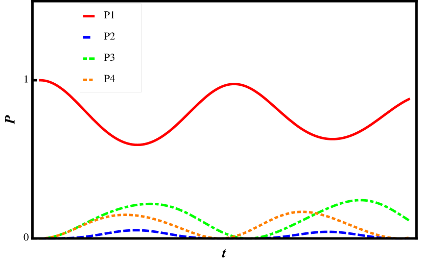
(a)

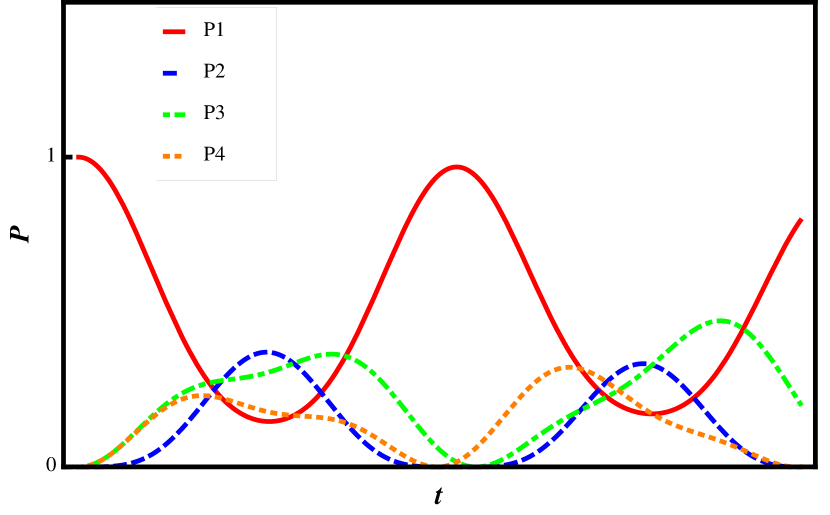
(b)

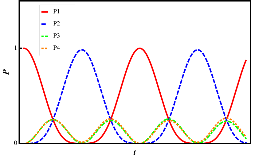
(c)

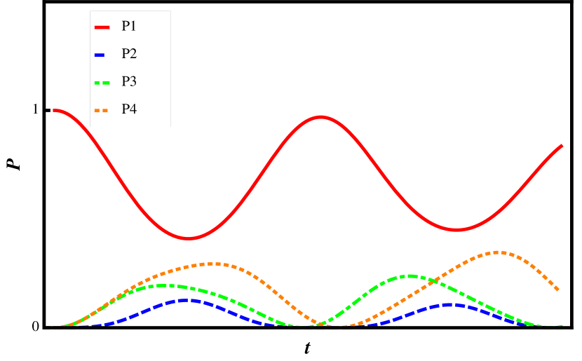
(d)

Figure 1: Survival probability $P1$ and spin flipping transition probabilities $P2$, $P3$, $P4$ to other spin states $|\psi_{2}\rangle$, $|\psi_{3}\rangle$, $|\psi_{4}\rangle$ for different values of $\theta$ as in (a) $\theta=0.5$, (b) $\theta=0.9$, (c) $\theta=1.6$, (d) $\theta=2.5$ as a function of time.

These plots confirm our previous assertion that if a rapidly decaying (with time) and inhomogeneous magnetic field exists, the evolution of spin states of quarkonia becomes nonadiabatic in the regime where the strength of the field is very weak. We have shown that this nonadiabaticity results in a dynamical spin mixing among all possible spin states of quarkonia, no matter which initial state we start with. However, the deconfined medium, once formed in HICs, might drag the magnetic field along with it and help it maintain an appreciably large value for quite some time Das et al. (2017). That being the scenario, the spin state evolution might have the possibility to be adiabatic and in turn, there will be no dynamical mixing occurring whatsoever. Hence, the manifestation or absence of this dynamical mixing among all the spin sates of quarkonia, as presented in this paper, can be a good way to decide the actual nature, strength and persistence of the magnetic field before and after the formation of the QCD medium in HICs.

References

- Skokov et al. (2009) V. Skokov, A. Yu. Illarionov, and V. Toneev, Int. J. Mod. Phys. A24, 5925 (2009), arXiv:0907.1396 [nucl-th] .
- Kharzeev et al. (2008) D. E. Kharzeev, L. D. McLerran, and H. J. Warringa, Nucl. Phys. A803, 227 (2008), arXiv:0711.0950 [hep-ph] .
- Rafelski and Muller (1976) J. Rafelski and B. Muller, Phys. Rev. Lett. 36, 517 (1976).
- Voronyuk et al. (2011) V. Voronyuk, V. D. Toneev, W. Cassing, E. L. Bratkovskaya, V. P. Konchakovski, and S. A. Voloshin, Phys. Rev. C83, 054911 (2011), arXiv:1103.4239 [nucl-th] .
- Kharzeev (2006) D. Kharzeev, Phys. Lett. B633, 260 (2006), arXiv:hep-ph/0406125 [hep-ph] .
- Bloczynski et al. (2013) J. Bloczynski, X.-G. Huang, X. Zhang, and J. Liao, Phys. Lett. B718, 1529 (2013), arXiv:1209.6594 [nucl-th] .
- Marasinghe and Tuchin (2011a) K. Marasinghe and K. Tuchin, Phys. Rev. C84, 044908 (2011a), arXiv:1103.1329 [hep-ph] .
- Bonati et al. (2015) C. Bonati, M. D’Elia, and A. Rucci, Phys. Rev. D92, 054014 (2015), arXiv:1506.07890 [hep-ph] .
- Guo et al. (2015) X. Guo, S. Shi, N. Xu, Z. Xu, and P. Zhuang, Phys. Lett. B751, 215 (2015), arXiv:1502.04407 [hep-ph] .
- Marasinghe and Tuchin (2011b) K. Marasinghe and K. Tuchin, Phys. Rev. C84, 044908 (2011b), arXiv:1103.1329 [hep-ph] .
- Karshenboim (2004) S. G. Karshenboim, Positronium physics. Proceedings, 1st International Workshop, Zuerich, Switzerland, May 30-31, 2003, Int. J. Mod. Phys. A19, 3879 (2004), arXiv:hep-ph/0310099 [hep-ph] .
- Filip (2013) P. Filip, Proceedings, 8th International Workshop on Critical Point and Onset of Deconfinement (CPOD 2013): Napa, CA, USA, March 11-15, 2013, PoS CPOD2013, 035 (2013).
- Alford and Strickland (2013) J. Alford and M. Strickland, Phys. Rev. D88, 105017 (2013), arXiv:1309.3003 [hep-ph] .
- Yang and Muller (2012) D.-L. Yang and B. Muller, J. Phys. G39, 015007 (2012), arXiv:1108.2525 [hep-ph] .
- Tuchin (2013) K. Tuchin, Phys. Rev. C88, 024911 (2013), arXiv:1305.5806 [hep-ph] .
- Das et al. (2017) A. Das, S. S. Dave, P. S. Saumia, and A. M. Srivastava, (2017), arXiv:1703.08162 [hep-ph] .
- Amin (2009) M. H. S. Amin, Phys. Rev. Lett. 102, 220401 (2009).
- Aharonov and Anandan (1987) Y. Aharonov and J. Anandan, Phys.Rev.Lett. 58, 1593 (1987).