Ringed accretion disks: evolution of double toroidal configurations

Abstract

We investigate ringed accretion disks constituted by two tori (rings) orbiting on the equatorial plane of a central super-massive Kerr black hole. We discuss the emergence of the instability phases of each ring of the macro-configuration (ringed disk) according to Paczynski violation of mechanical equilibrium. In the full general relativistic treatment, we consider the effects of the geometry of the Kerr spacetimes relevant in the characterization of the evolution of these configurations. The discussion of the rings stability in different spacetimes enables us to identify particular classes of central Kerr attractors in dependence of their dimensionless spin. As a result of this analysis we set constraints of the evolutionary schemes of the ringed disks related to the tori morphology and their rotation relative to the central black hole and to each other. The dynamics of the unstable phases of this system is significant for the high energy phenomena related to accretion onto super-massive black holes in active galactic nuclei (AGNs), and the extremely energetic phenomena in quasars which could be observable in their X-ray emission.

=1 The Friends of AASTeX Collaboration

1 Introduction

The physics of accretion disks around super-massive attractors is characterized by several processes of very diversified nature and it is ground of many phenomena of the high energy astrophysics. However, the existence of a unique satisfactory framework for a complete theoretical interpretation of such observations remains still to be proved, as the phenomenology associated with these systems includes very different events all supposedly related to the physics of strong attractors and their environment: from the issue of jet generation and collimation, to the Gamma-ray bursts (GRBs) and the accretion process itself. Particularly, accretion of matter from disks orbiting super-massive black holes (SMBHs), hosted in the centre of active galactic nuclei (AGN) or quasars, is a subject which seems to require consistent additional investigations. The location and definition of the inner edge of an accretion disk for example is one of the topics that are continuously debated within several argumentations leading often to different conclusions (Krolik&Hawley, 2002; Bromley et al., 1998; Abramowicz et al., 2010; Agol&Krolik, 2000; Paczyński, 2000). The interaction between the SMBHs and orbiting matter is certainly a complicated subject of investigation which entangles the central attractor and the embedded material in one dynamical picture. Interaction between the attractor and environment could give rise potentially to a mutation of the geometrical characteristics of spacetime which, initially considered as “frozen background”, may change following a spin-down or eventually spin-up of the non isolated black hole (BH)(Abramowicz et al., 1983, 1998; Rezzolla et al., 2003; Font&Daigne, 2002a; Hamersky&Karas, 2013; Korobkin et al., 2013). Jets emission is then a further key element of such systems: the relation between the rotational energy of the central attractor, disk inner edge location and jet emission (jet-accretion correlation) is still substantially obscure(Lovelace et al., 2014; McKinney et al., 2013; Allen et al., 2006; Stuchlík&Kolos, 2016; Marscher et al., 2002; Maraschi&Tavecchio, 2003; Chen et al., 2015; Yu et al., 2015; Zhang et al., 2015; Sbarrato et al., 2014; Coughlin&Begelman, 2014; Maitra et al., 2009; Fender&Munoz-Darias, 2015; Abramowicz&Sharp, 1983; Sadowski&Narayan, 2015; Okuda et al., 2005; Ferreira&Casse, 2004; Lyutikov, 2009; Ghisellini et al., 2014; Fragile et al., 2012).

However, considering the huge variety of approaches and studies on each of these individual issues, it appears necessary, in addressing these topics, to formulate the investigation in a more global perspective reformulating the problem in terms of structures and macro-structures, the first understood as isolated objects the second as isolated clusters of individual interacting objects, to consider the relation between the different components in these systems, and involving the knowledge acquired on certain specific processes such as the accretion mechanism, jet properties and black hole physics in a more inclusive picture.

Accretion disk models may be distinguished by at least three important aspects: the geometry (the vertical thickness defines geometrically thin or thick disks), the matter accretion rate (sub or super-Eddington luminosity), and the optical depth (transparent or opaque disks)–see (Abramowicz&Fragile, 2013). Geometrically thick disks are well modelled as the Polish Doughnuts (P-D) (Kozlowski et al., 1978; Abramowicz et al., 1978; Jaroszynski et al., 1980; Stuchlík et al., 2000; Rezzolla et al., 2003; Slaný&Stuchlík, 2005; Stuchlik, 2005; Pugliese et al., 2012; Pugliese&Montani, 2013b), or also the ion tori (Rees et al., 1982). The P-D tori (with very high, super-Eddington, accretion rates) and slim disks have high optical depth while the ion tori and the ADAF (Advection-Dominated Accretion Flow) disks have low optical depth and relatively low accretion rates (sub-Eddington). Geometrically thin disks are generally modelled as the standard Shakura-Sunayev (Keplerian) disks (Shakura, 1973; Shakura&Sunyaev, 1973; Novikov&Thorne, 1973; Page&Thorne74, 1974), the ADAF disks (Abramowicz&Straub, 2014; Narayan et al., 1998), and the slim disks (Abramowicz&Fragile, 2013). In these disks, dissipative viscosity processes are relevant for accretion, being usually attributed to the magnetorotational instability of the local magnetic fields (Hawley et al., 1984; Hawley, 1987, 1991; De Villiers&Hawley, 2002). On the other hand in the toroidal disks, pressure gradients are crucial (Abramowicz et al., 1978). As proposed in (Paczyński, 1980), accretion disks can been modelled by using an appropriately defined Pseudo-Newtonian potential, see also (Novikov&Thorne, 1973; Abramowicz et al., 1978; Stuchlik, 2005; Stuchlík et al., 2009; Abramowicz&Fragile, 2013).

In Pugliese&Stuchlík (2015) we considered the possibility that during several accretion regimes occurred in the lifetime of non isolated super-massive Kerr black hole several toroidal fluid configurations might be formed from the interaction of the central attractor with the environment in AGNs, where corotating and counterrotating accretion stages are mixed (Dyda et al., 2015; Alig et al., 2013; Carmona-Loaiza et al., 2015; Lovelace&Chou, 1996; Gafton et al., 2015). These systems can be then reanimated in some subsequent stages of the BH-accretion disks life, for example in colliding galaxies, or in galactic center, in some kinds of binary systems, where some additional matter could be supplied into the vicinity of the central black hole due to tidal distortion of a star, or if some cloud of interstellar matter is captured by the strong gravity.

We formulated an analytic model of a macro-structure, the ringed accretion disk, made by several toroidal axis-symmetric sub-configurations (rings) of corotating and counterrotating fluid structures (tori) orbiting one center super-massive Kerr black hole, with symmetry plane coinciding with the equatorial plane of the central Kerr BH. The emergence of instabilities for each ring and the entire macro-structure was then addressed in Pugliese&Stuchlík (2016a, b). Similar studies on analogue problems are in Cremaschini et al. (2013) where off-equatorial tori around compact objects were considered and also in Nixon et al. (2012b). In Pugliese&Stuchlík (2016c) we drew some conclusions for the case of only two toroidal disks orbiting a central Kerr attractor. We demonstrated that only under specific conditions a double accretion system may be formed. Rings of the macro-structure can then interact colliding. The center-of-mass energy during ring collision was evaluated within the test particle approximation demonstrating that energy efficiency of the collisions increases with increasing dimensionless black hole spin, being very high for near-extreme black holes. The collisional energy efficiency could be even higher in near-extreme Kerr naked singularity spacetimes Stuchlík&Schee (2013, 2012); Stuchlik (1980).

Using numerical methods, multi-disks have been also analyzed in more complex, non-symmetric situations. Formation of several accretion disks in the geometries of the SMBH in AGNs or in binary systems, have been considered in relation to various factors, where the rupture of symmetries has been addressed, for example for titled, warped, not coplanar disks. Attention has been paid to the investigations of the relevance of the disk geometry in the attractor-disk interaction. Initial stages of the formation of such systems has been addressed in Ansorg et al (2003). Concerning counter-aligned accretion disks in AGN, we point out King&Pringle (2006), where the Bardeen-Petterson effect is proposed as a possible cause of the counter-alignment of BH and disk spins: it is shown that BH can grow rapidly if they acquire most of accreting mass it in a sequence of randomly oriented accretion episodes. In Lodato&Pringle (2006), the evolution of misaligned accretion disks and spinning BH are considered especially in AGN, where the BH spin changes under the action of the disk torques, as the disk, being subjected to Lense-Thirring precession, becomes twisted and warped. It is shown that accretion from misaligned disk in galactic nuclei would be significantly more luminous than accreting from a flat disk. Aligning of Kerr BHs and accretion disks are studied in King et al. (2005). In Nealon et al. (2015) the effects of BH spin on warped or misaligned accretion disks are studied in connections to the role of the inner edge of the disk in the alignment of the angular momentum with the BH spin. Stable counter-alignment of a circumbinary disk is focused in Nixon (2012). King et al. (2008) argue that there is a generic tendency of AGN accretion disks to become self-gravitating at a certain radius from the attractor. The study of particular accretion processes including merging of the AGN accretion disk, demonstrates that the disk has generally a lower angular momentum than the BH, for an analogue limit in Pugliese&Montani (2015). The chaotical accretion in AGNs could produce counter rotating accretion disks or strongly misaligned disks with respect to the central SMBH spin. Rapid AGN accretion from counter rotating disks is particularly addressed in Nixon et al. (2012a). Authors studied the angular momentum cancelation in accretion disks characterized by a significant tilt between inner and outer disk parts. These studies show that evolution of a misaligned disks around a Kerr BH might lead to a tearing up of the disk into several planes with different inclinations. Tearing up the disk in misaligned accretion onto a binary system is considered for example in Nixon et al. (2013).

Tearing up process has been also considered as possible mechanism behind the almost periodic emission in X-ray emission band known as QPOs. Tearing up a misaligned accretion disk with a binary companion is addressed in Dogan et al. (2015). disk formation by tidal disruptions of stars on eccentric orbits by a spherically symmetric black hole is considered in Bonnerot et al. (2016). For misaligned gas disks around eccentric BHs binaries see Aly et al. (2015).

As explained in Nixon et al. (2012b), in realistic cases of AGN accretion, or also in stellar-mass X-ray binaries, there is a break in the central part of a tilted accretion disks orbiting Kerr BHs due to the Lense-Thirring effect. The disk is thus splitted into several, essentially separated, planes. It is observed that also for small tilt angles the disk may still break and this must be connected with some observable phenomena as for example QPOs. For a brief review of the SMBH accretion mergers and accretion flows on to SMBH see King&Nixon (2013).

The existence of ringed disks in general may lead us to reinterpret action of the phenomena so far analyzed in a single disk framework in terms of orbiting multi-toroidal structures. Especially, this shift could be reinforced in modelling the spectral features of multi-disk structures. It is generally assumed that the X-ray emission from AGNs is related to accretion disks and surrounding corona. Assuming to be related to the accretion disk instabilities, the spectra interpretation of X-ray emission is taken to constrain the main BH-disk model parameters. We argue that this spectra profile should provide also a fingerprint of the ringed disk structure, possibly showing as a radially stratified emission profile. In fact, the simplest structures of this kind are thin radiating rings. Signature of alternative gravity, as exotic objects, given by spectral lines from the radiating rings is investigated in Schee&Stuchlik (2009, 2013); Bambi et al. (2016); Ni et al. (2016). In Sochora et al. (2011) the authors propose that the BH accretion rings models may be revealed by future X-ray spectroscopy, from the study of relatively indistinct excesses on top of the relativistically broadened spectral line profile, unlike the main body of the broad line of the spectral line profile, connected to an extended (continuous) region of the accretion disk. They predicted relatively indistinct excesses of the relativistically broadened emission-line components, arising in a well-confined radial distance in the accretion disk, envisaging therefore a sort of rings model which may be adapted as a special case of the model discussed in Pugliese&Stuchlík (2015, 2016a). Specifically, in Karas&Sochora (2010) extremal energy shifts of radiation from a ring near a rotating black hole were particularly studied: radiation from a narrow circular ring shows a double-horn profile with photons having energy around the maximum or minimum of the range (see also Schee&Stuchlik (2009)). This energy span of spectral lines is a function of the observer’s viewing angle, the black hole spin and the ring radius. The authors describe a method to calculate the extremal energy shift in the regime of strong gravity. The accretion disk is modelled by a rings located in a Kerr BH equatorial plane, originating by a series of episodic accretion events. It is argued that the proposed geometric and emission ringed structure should be evident from the extremal energy shifts of the each rings. Accordingly, the ringed disks may be revealed thought detailed spectroscopy of the spectral line wings. Although the method has been specifically adapted to the case of geometrically thin disks, an extension to thick rings should be possible. Furthermore, as detailed in Pugliese&Stuchlík (2016a, 2015), some of the general geometric characteristics of the ringed disk structure are well applicable to the thin disk case.

Here we extend the study in Pugliese&Stuchlík (2015, 2016a) considering an orbiting pair of axi-symmetric tori governed by the relativistic hydrodynamic Boyer condition of equilibrium configurations of rotating perfect fluids Boyer (1965). Our primary result is the characterization the rings-attractor systems in terms of equilibrium or unstable (critical) topology, constraining the formation of such a system on the basis of the (frozen) dimensionless spin-mass ratio of the attractor and the relative rotation of the fluids. We investigate the possible dynamical evolution of the tori, generally considered as transition from the topological state of equilibrium to a topology of instability, and the evolution for the entire macro-configuration when accretion onto the central black hole and collision among the tori may occur. We enlighten the situation where tori collisions lead to the destruction of the macro-configuration. We summarized this analysis developing some evolutionary schemes which provide indications of the topology transition and the situations where these systems could potentially be found and then observed due to the associated phenomena. These schemes are constrained by spin of the attractor and the relative rotation of the rings with respect to attractor or each other. From the methodological viewpoint we represented evolutionary schemes with graph models, which we consider here also as reference in our discussion.

In our model we primarily evaluate the general relativistic effects on the orbiting matter in those situations where curvature effects and the fluid rotation are considerable in determination of the toroidal topology and morphology. We focus on toroidal disk model orbiting the super-massive Kerr attractors using the geometrically thick disk as Polish Doughnuts (P-D), opaque and with very high (super-Eddington) accretion rates where pressure gradients are crucial (Kozlowski et al., 1978; Abramowicz et al., 1978; Jaroszynski et al., 1980; Stuchlík et al., 2000; Rezzolla et al., 2003; Slaný&Stuchlík, 2005; Stuchlik, 2005; Pugliese et al., 2012). These configurations are often adopted as the initial conditions in the set up for simulations of the MHD (magnetohydrodynamic) accretion structures(Igumenshchev, 2000; Fragile et al., 2007; De Villiers&Hawley, 2002). In fact, the majority of the current analytical and numerical models of accretion configurations assumes the axial symmetry of the extended accreting matter.

For the geometrically thick configurations it is generally assumed that the time scale of the dynamical processes $\tau_{dyn}$ (regulated by the gravitational and inertial forces, the timescale for pressure to balance the gravitational and centrifugal force) is much lower than the time scale of the thermal ones $\tau_{the}$ (i.e. heating and cooling processes, timescale of radiation entropy redistribution) that is lower than the time scale of the viscous processes $\tau_{vis}$, and the effects of strong gravitational fields are dominant with respect to the dissipative ones and predominant to determine the unstable phases of the systems (Font&Daigne, 2002b; Igumenshchev, 2000; Abramowicz&Fragile, 2013), i.e. $\tau_{dyn}\ll\tau_{the}\ll\tau_{vis}$ see also Fragile et al. (2007); De Villiers&Hawley (2002); Hawley (1987, 1991); Hawley et al. (1984). This in turn grounded the assumption of perfect fluid energy-momentum tensor. Thus the effects of strong gravitational fields dominate the dissipative ones (Font&Daigne, 2002b; Abramowicz&Fragile, 2013; Paczyński, 1980). Consequently during the evolution of dynamical processes, the functional form of the angular momentum and entropy distribution depends on the initial conditions of the system and on the details of the dissipative processes. Paczyński realized that it is physically reasonable to assume an ad hoc distributions Abramowicz (2008). This feature constitutes a great advantage of these models and render their adoption extremely useful and predictive (the angular momentum transport in the fluid is perhaps one of the most controversial aspects in thin accretion disk). Moreover, we should note that the Paczyński accretion mechanics from a Roche lobe overflow induces the mass loss from tori being an important local stabilizing mechanism against thermal and viscous instabilities, and globally against the Papaloizou-Pringle instability (for a review we refer to Abramowicz&Fragile (2013)).

In this models the entropy is constant along the flow. According to the von Zeipel condition, the surfaces of constant angular velocity $\Omega$ and of constant specific angular momentum $\ell$ coincide (Abramowicz, 1971; Chakrabarti, 1990, 1991; Zanotti&Pugliese, 2015) and the rotation law $\ell=\ell(\Omega)$ is independent of the equation of state (Lei et al., 2008; Abramowicz, 2008).

Article layout

In details the plan of this article is as follows: The introduction of the thick accretion disks model in a Kerr spacetime is summarized in Section (2) where the main notation considered through this work is presented. This section constitutes first introductive part of this work and also the disclosure of the methodological tools used throughout. We provide main definitions of the major morphological features of the ringed disks. Then, we specialize the concepts for the case of system composed by only two tori. After writing the Euler equations for the orbiting fluids we cast the set of hydrodynamic equations for the tori by introducing an effective potential function for the macro-configuration. We then investigate the parameter space for this model; one set of couple parameters provides the boundary conditions for the description of two tori in the macro-configuration. We proceed by dividing the discussion for the $\ell$corotating and $\ell$counterrotating tori-if the tori are both corotating or counterrotating with respect to the central Kerr BH they are $\ell$corotating, if one torus is corotating and the other counterrotating they are $\ell$counterrotating. However, even in the case of one couple of tori orbiting around a single central Kerr BH, a remarkably large number of possible configurations is possible. Therefore, in order to simplify and illustrate the discussion, we made use of special graphs for the representation of a couple of accretion tori and their evolution, within the constraints they are subjected to. The use of these graphic schemes has been reveled to be crucial for the study and representation of these evolutionary cases. Although the following analysis may be followed quite independently from the graph formalism, they can be used also to quickly collect the different constraints on the existence and evolution of the tori and for reference in our discussion. Therefore we include here also a brief description of the graph construction and basic concepts related to these structures. Appendix (A) discloses details on the construction and interpretation of graphs. Main graph blocks are listed in Fig. (6). The main analysis of the present work is in Section (3), where the double tori disk system is discussed in details. We specialize the investigation detailing the double system on the basis of relative rotation of fluids in the disks and with respect to the central BH attractor; therefore in Sec. (3.1) the $\ell$corotating couple of tori is addressed while in Sec. (3.2) we focus attention on the $\ell$counterrotating case. We shall see that the results of Section (3.1) also apply to the description of $\ell$counterrotating tori in a Schwarzschild (static) spacetime. The double tori disk system is characterized by the existence and stability conditions. We consider first all the possible states for the couple of accretion disks with fixed topology, and then we concentrate on their evolutions. We will prove that some configurations are prohibited. Then we narrow the space of the system parameters to specific regions according to the dimensionless BH spin. The case of $\ell$counterrotating couples around a rotating attractor is in fact much more articulated in comparison to $\ell$corotating (or $\ell$counterrotating torii orbiting a Schwarzschild black hole). This case is hugely diversified for classes of attractors, and for the disk spin orientation with respect to the central attractor. Therefore it requested a different approach adapted to the diversification of the cases. In order to better analyze the situation we have split the analysis in the two sub-sections (3.2.1) and (3.2.2); in the first we consider the case in which the inner torus of the couple is counterrotating with respect to the attractor, then we address the inner corotating torus. The accurate analysis in the space of parameter also allows us to discuss the possible and forbidden lines of evolution for a fixed couple. We close Section (3) in the Section (3.3) where the possibility of collision between tori and the possibility of tori merging is considered. We investigate the conditions for collision occurrence, drowning a description of the associated unstable macro-configurations. Both $\ell$corotaing and $\ell$counterrotating cases are addressed. We discuss mechanisms which may lead to tori collision according to our model prescription. This section also refers to the Appendix (A.1), where further details are provided. Indications on possible observational evidence of doubled tori disks and their evolution are provided in brief Section (4). We close this article in Sec. (5) with a summary and brief discussion of future prospectives. Appendix (A) and Appendix (B) follow.

2 Thick accretion disks in a Kerr spacetime

The Kerr metric line element in the Boyer-Lindquist (BL) coordinates $\{t,r,\theta,\phi\}$ reads

$$ds^{2}=-dt^{2}+\frac{\rho^{2}}{\Delta}dr^{2}+\rho^{2}d\theta^{2}+(r^{2}+a^{2})\sin^{2}\theta d\phi^{2}+\frac{2M}{\rho^{2}}r(dt-a\sin^{2}\theta d\phi)^{2}\ ,$$ (1)

$$\mbox{where}\quad\rho^{2}\equiv r^{2}+a^{2}\cos\theta^{2}\quad\mbox{and }\quad\Delta\equiv r^{2}-2Mr+a^{2},$$

and $a=J/M\in]0,M]$ is the specific angular momentum, $J$ is the total angular momentum of the gravitational source and $M$ is the gravitational mass parameter. The horizons $r_{-}<r_{+}$ and the outer static limit $r_{\epsilon}^{+}$ are respectively given by:

$$r_{\pm}\equiv M\pm\sqrt{M^{2}-a^{2}};\quad r_{\epsilon}^{+}\equiv M+\sqrt{M^{2}-a^{2}\cos\theta^{2}};$$ (2)

where $r_{+}<r_{\epsilon}^{+}$ on $\theta\neq 0$ and $r_{\epsilon}^{+}=2M$ in the equatorial plane $\theta=\pi/2$. The non-rotating limiting case $a=0$ is the Schwarzschild metric while the extreme Kerr black hole has dimensionless spin $a/M=1$. In the Kerr geometry the quantities

$${E}\equiv-g_{\alpha\beta}\xi_{t}^{\alpha}p^{\beta}=-p_{t},\quad L\equiv g_{\alpha\beta}\xi_{\phi}^{\alpha}p^{\beta}=p_{\phi}\ ,$$ (3)

are constants of motion, where $\xi_{\phi}=\partial_{\phi}$ is the rotational Killing field, $\xi_{t}=\partial_{t}$ is the Killing field representing the stationarity of the spacetime, and $p^{\alpha}$ is the particle four–momentum. The constant $L$ in Eq. (3) may be interpreted as the axial component of the angular momentum of a test particle following timelike geodesics and $E$ is representing the total energy of the test particle coming from radial infinity, as measured by a static observer at infinity. Due to the symmetries of the metric tensor (1), the test particle dynamics is invariant under the mutual transformation of the parameters $(a,L)\rightarrow(-a,-L)$, and we could restrict the analysis of the test particle circular motion to the case of positive values of $a$ for corotating $(L>0)$ and counterrotating $(L<0)$ orbits.

In this work we specialize our analysis to toroidal configurations of perfect fluid orbiting a Kerr black hole (BH) attractor. The energy momentum tensor for one-species particle perfect fluid system is described by

$$T_{\alpha\beta}=(\varrho+p)u_{\alpha}u_{\beta}+\ pg_{\alpha\beta},$$ (4)

where $u^{\alpha}$ is a timelike flow vector field and $\varrho$ and $p$ are the total energy density and pressure respectively, as measured by an observer comoving with the fluid with velocity $u^{\alpha}$. For the symmetries of the problem, we assume $\partial_{t}\mathbf{Q}=0$ and $\partial_{\varphi}\mathbf{Q}=0$, with $\mathbf{Q}$ being a generic spacetime tensor. According to these assumptions the continuity equation is identically satisfied and the fluid dynamics is governed by the Euler equation:

$$(p+\varrho)u^{\alpha}\nabla_{\alpha}u^{\gamma}+\ h^{\beta\gamma}\nabla_{\beta}p=0\,,$$ (5)

where $\nabla_{\alpha}g_{\beta\gamma}=0$, $h_{\alpha\beta}=g_{\alpha\beta}+u_{\alpha}u_{\beta}$ is the projection tensor (Pulgiese&Kroon, 2012; Pugliese&Montani, 2015). Assuming a barotropic equation of state $p=p(\varrho)$, and orbital motion with $u^{\theta}=0$ and $u^{r}=0$, Eq. (5) implies

$$\frac{\partial_{\mu}p}{\varrho+p}=-{\partial_{\mu}W}+\frac{\Omega\partial_{\mu}\ell}{1-\Omega\ell},\quad\ell\equiv\frac{L}{E},\quad W\equiv\ln V_{eff}(\ell),\quad V_{eff}(\ell)=u_{t}=\pm\sqrt{\frac{g_{\phi t}^{2}-g_{tt}g_{\phi\phi}}{g_{\phi\phi}+2\ell g_{\phi t}+\ell^{2}g_{tt}}},$$ (6)

where $\Omega=u^{\phi}/u^{t}$ is the relativistic angular frequency of the fluid relative to the distant observer, and the Pacz y ński-Wiita (P-W) potential $W(r;\ell,a)$ and the effective potential for the fluid $V_{eff}(r;\ell,a)$ were introduced. These functions of position reflect the background Kerr geometry through the parameter $a$, and the centrifugal effects through the fluid specific angular momenta $\ell$, here assumed constant and conserved (see also (Lei et al., 2008; Abramowicz, 2008)). A natural extremal limit on the extension of both corotating and counterrotating tori occurs due to the cosmic repulsion at the so called static radius that is independent of the black hole spin (Stuchlík et al., 2009; Slaný&Stuchlík, 2005; Stuchlik et al., 2005; Stuchlík et al., 2000; Stuchlik&Hledik, 1999; Stuchlik, 1983, 2005).

The effective potential in Eq. (6) is invariant under the mutual transformation of the parameters $(a,\ell)\rightarrow(-a,-\ell)$. Therefore analogously to the analysis of test particle dynamics, we can assume $a>0$ and consider $\ell>0$ for corotating and $\ell<0$ for counterrotating fluids, within the notation $(\mp)$ respectively.

The ringed accretion disks, introduced in Pugliese&Montani (2015); Pugliese&Stuchlík (2015, 2016a), represent a fully general relativistic model of toroidal disk configurations $\mathbf{C}^{n}=\bigcup^{n}\mathrm{C}_{i}$, consisting of a collection of $n$ sub-configurations (configuration order $n$) of corotating and counterrotating toroidal rings orbiting a supermassive Kerr attractor–Figs (3). Since tori can be corotating or counterrotating with respect to the black hole, assuming first a couple $(\mathrm{C}_{a},\mathrm{C}_{b})$, orbiting in the equatorial plane of a given Kerr BH with specific angular momentum $(\ell_{a},\ell_{b})$, we need to introduce the concept of $\ell$corotating disks, defined by the condition $\ell_{a}\ell_{b}>0$, and $\ell$counterrotating disks defined by the relations $\ell_{a}\ell_{b}<0$. The two $\ell$corotating tori can be both corotating, $\ell a>0$, or counterrotating, $\ell a<0$, with respect to the central attractor–see Fig. (4).

The construction of the ringed configurations is actually independent of the adopted model for the single accretion disk (sub-configuration or ring). However, to simplify discussion we consider here each toroid of the ringed disk governed by the General Relativity hydrodynamic Boyer condition of equilibrium configurations of rotating perfect fluids. We will see that in situations where the curvature effects of the Kerr geometry are significant, results are largely independent of the specific characteristics of the model for the single disk configuration, being primarily based on the characteristics of the geodesic structure the Kerr spacetime related to the matter distribution. This is a geometric property consisting of the union of the orbital regions with boundaries at the notable radii $\mathbf{R}_{\mathrm{N}}^{\pm}\equiv\{r_{\gamma}^{\pm},r_{\mathrm{mbo}}^{\pm},r_{\mathrm{mso}}^{\pm}\}$. It can be decomposed, for $a\neq 0$, into $\mathbf{R}_{\mathrm{N}}^{-}$ for the corotating and $\mathbf{R}_{\mathrm{N}}^{+}$ for counterrotating matter. Specifically, for timelike particle circular geodetical orbits, $r_{\gamma}^{\pm}$ is the marginally circular orbit or the photon circular orbit, timelike circular orbits can fill the spacetime region $r>r_{\gamma}^{\pm}$. The marginally stable circular orbit $r_{\mathrm{mso}}^{\pm}$: stable orbits are in $r>r_{\mathrm{mso}}^{\pm}$ for counterrotating and corotating particles respectively. The marginally bounded circular orbit is $r_{\mathrm{mbo}}^{\pm}$, where $E_{\pm}(r_{\mathrm{mbo}}^{\pm})=1$ (Pugliese et al., 2011b, 2013, a; Pugliese&Quevedo, 2015; Stuchlik, 1981a, b; Stuchlik&Kotrlova, 2008; Stuchlik&Slany, 2003) –see Fig. (1) and Fig. (2). Given $r_{i}\in\mathcal{R}$, we adopt the following notation for any function $\mathbf{Q}(r):\;\mathbf{Q}_{i}\equiv\mathbf{Q}(r_{i})$, for example $\ell_{\mathrm{mso}}^{+}\equiv\ell_{+}(r_{\mathrm{mso}}^{+})$ and, more generally, given the radius $r_{\bullet}$ and the function $\mathbf{Q}(r)$, there is $\mathbf{Q}_{\bullet}\equiv\mathbf{Q}(r_{\bullet})$. Since the intersection set of $r_{\mathrm{N}}^{\pm}$ is not empty, the character of the geodesic structure will be particularly relevant in the characterization of the $\ell$counterrotating sequences(Pugliese&Stuchlík, 2015).

According to the Boyer theory on the equipressure surfaces applied to a P-D torus, the toroidal surfaces are the equipotential surfaces of the effective potential $V_{eff}(\ell,r)$, being solutions of $V_{eff}=K=$constant or $\ln(V_{eff})=\rm{c}=\rm{constant}$ (Boyer, 1965; Kozlowski et al., 1978). These correspond also to the surfaces of constant density, specific angular momentum $\ell$, and constant relativistic angular frequency $\Omega$, where $\Omega=\Omega(\ell)$ as a consequence of the von Zeipel theorem (Abramowicz, 1971; Zanotti&Pugliese, 2015; Kozlowski et al., 1978). Then, each Boyer surface is uniquely identified by the couple of parameters $\mathbf{p}\equiv(\ell,K)$. We focus on the solution of Eq. (6), $W=$constant, associated to the critical points of the effective potential, assuming constant specific angular momentum and parameter $K$. Considering $\Delta_{crit}\equiv[r_{\max},r_{\min}]$, whose boundaries correspond to the maximum and minimum points of the effective potential respectively, we have that the centers $r_{cent}$ of the closed configurations $\mathrm{C}_{\pm}$ are located at the minimum points $r_{\min}>r_{\mathrm{mso}}^{\pm}$ of the effective potential, where the hydrostatic pressure reaches a maximum. The toroidal surfaces are characterized by $K_{\pm}\in[K^{\pm}_{\min},K^{\pm}_{\max}[\subset]K_{\mathrm{mso}}^{\pm},1[\equiv\mathbf{K0}$ and momentum $\ell_{\pm}\lessgtr\ell_{\mathrm{mso}}^{\pm}\lessgtr 0$ respectively. The inner edge of the Boyer surface is at $r_{in}\in\Delta_{crit}$, or $r_{in}\equiv y_{3}$ on the equatorial plane, the outer edge is at $r_{out}>r_{\min}$, or $r_{out}\equiv y_{1}$ on the equatorial plane as in Fig. (3). A further matter configuration closest to the black hole is at $r_{in}<r_{\max}$. The limiting case of $K_{\pm}=K_{\min}^{\pm}$ corresponds to a one-dimensional ring of matter located in $r_{\min}^{\pm}$. Equilibrium configurations, with topology $\mathrm{C}$, exist for $\pm\ell_{\mp}>\pm\ell_{\mathrm{mso}}^{\mp}$ centered in $r>r_{\mathrm{mso}}^{\mp}$, respectively. In general, we denote by the label $(i)$, with $i\in\{1,2,3\}$ respectively, any quantity $\mathbf{Q}$ related to the range of specific angular momentum $\mathbf{Li}$ respectively; for example, $\mathrm{C}_{1}^{+}$ indicates a closed regular counterrotating configuration with specific angular momentum $\ell_{1}^{+}\in\mathbf{L1}^{+}$.

The local maxima of the effective potential $r_{\max}$ correspond to minimum points of the hydrostatic pressure and the P-W points of gravitational and hydrostatic instability. No maxima of the effective potential exist for $\pm\ell_{\mp}>\ell_{\gamma}^{\pm}$ ($\mathbf{L3}^{\mp}$) therefore, only equilibrium configurations $\mathrm{C}_{3}$ are possible. An accretion overflow of matter from the closed, cusped configurations in $\mathrm{C}^{\pm}_{\times}$ (see Fig. (3)) towards the attractor can occur from the instability point $r^{\pm}_{\times}\equiv r_{\max}\in]r_{\mathrm{mbo}}^{\pm},r_{\mathrm{mso}}^{\pm}[$, if $K_{\max}\in\mathbf{K0}^{\pm}$ with specific angular momentum $\ell\in]\ell_{\mathrm{mbo}}^{+},\ell_{\mathrm{mso}}^{+}[\equiv\mathbf{L1}^{+}$ or $\ell\in]\ell_{\mathrm{mso}}^{-},\ell_{\mathrm{mbo}}^{-}[\equiv\mathbf{L1}^{-}$. Otherwise, there can be funnels of material along an open configuration $\mathrm{O}^{\pm}_{\times}$, proto-jets or for brevity jets, which represent limiting topologies for the closed surfaces (Kozlowski et al., 1978; Sadowski et al., 2016; Lasota et. al., 2016; Lyutikov, 2009; Madau, 1988; Sikora, 1981) with $K^{\pm}_{\max}\geq 1$ ($\mathbf{K1}^{\pm}$), “launched” from the point $r^{\pm}_{\mathrm{J}}\equiv r_{\max}\in]r_{\gamma}^{\pm},r_{{\mathrm{mbo}}}^{\pm}]$ with specific angular momentum $\ell\in]\ell_{\gamma}^{+},\ell_{\mathrm{mbo}}^{+}[\equiv\mathbf{L2}^{+}$ or $]\ell_{\mathrm{mbo}}^{-},\ell_{\gamma}^{-}[\equiv\mathbf{L2}^{-}$.

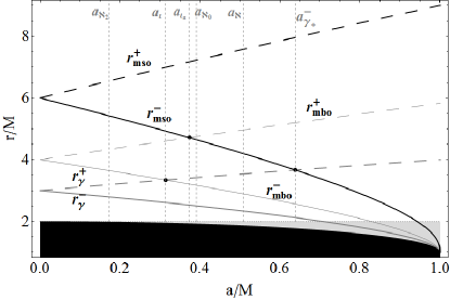
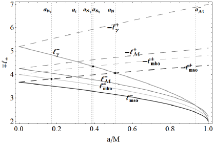
Figure 1: Geodesic structure of the Kerr geometry: notable radii $\mathbf{R}_{\mathrm{N}}\equiv\{r_{\gamma}^{\pm},r_{\mathrm{mbo}}^{\pm},r_{\mathrm{mso}}^{\pm}\}$ (left panel), and the respective fluid specific angular momentum $\ell^{\pm}_{i}=\ell^{\pm}(r^{\pm}_{i})$ where $r^{\pm}_{i}\in\{\mathbf{R}_{\mathrm{N}}^{\pm},r_{\mathcal{M}}^{\pm}\}$, $r_{\mathcal{M}}^{\pm}$ is the maximum point of derivative $\partial_{r}(\mp\ell^{\pm})$ for $a/M$ respectively. Some notable spacetime spin-mass ratios are also plotted, a list can found in Table (1). Black region is $r<r_{+}$, $r_{+}$ being the outer horizon of the Kerr geometry, gray region is $r<r_{\epsilon}^{+}$, $r_{\epsilon}^{+}$ is the outer ergosurface.

However, we can locate the points of maximum pressure, which correspond to the center of each torus, at $r^{\pm}_{\min}>r_{\mathrm{mso}}^{\pm}$ more precisely, by introducing the “complementary” geodesic structure, associated to the geodesic structure constituted by the notable radii $\mathbf{R}_{\mathrm{N}}$, by defining the radii $\bar{\mathfrak{r}}_{\mathrm{N}}\in\bar{\mathbf{{R}}}_{\mathrm{N}}:$ $\bar{\mathfrak{r}}_{\mathrm{N}}>{r}_{\mathrm{N}}$ solutions of $\bar{\ell}_{\mathrm{N}}\equiv\ell(\bar{\mathfrak{r}}_{\mathrm{N}})=\ell(r_{\mathrm{N}})\equiv\ell_{\mathrm{N}}$–see Fig. (1) and Fig. (2).

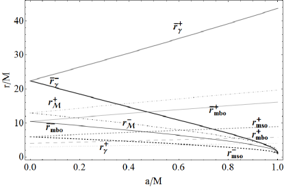
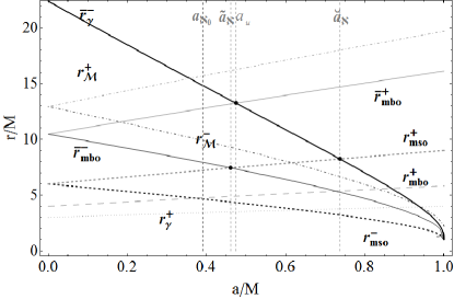
Figure 2: Geodesic structure of the Kerr geometry: notable radii $\mathbf{R}_{\mathrm{N}}\equiv\{r_{\gamma}^{\pm},r_{\mathrm{mbo}}^{\pm},r_{\mathrm{mso}}^{\pm}\}$ and complementary geodesic structure $\overline{\mathbf{R}}_{\mathrm{N}}\equiv\{\bar{\mathfrak{r}}_{\gamma}^{\pm},\bar{\mathfrak{r}}_{\mathrm{mbo}}^{\pm},\bar{\mathfrak{r}}_{\mathrm{mso}}^{\pm}\}$. Some notable spacetime spin-mass ratios are also plotted, a list can found in Table (1). Orbits $\bar{r}_{\mathrm{N}}>{r_{{\mathrm{N}}}}:\;\ell(\bar{\mathfrak{r}}_{\mathrm{N}})=\ell({r_{\mathrm{N}}})\equiv\ell_{\mathrm{N}}$ where $r_{\mathrm{N}}\in\mathbf{R}_{\mathrm{N}}$. The only solution at $a\neq 0$ of $\bar{\mathfrak{r}}_{\mathrm{N}}={r_{{\mathrm{N}}}}$ is the marginally stable orbit $r_{\mathrm{mso}}^{\pm}$ respectively. The radii $r_{\mathcal{M}}^{\pm}$ is the maximum point of derivative $\partial_{r}(\mp\ell^{\pm})$ for $a/M$ respectively. Right panel show a limited orbital range at $r\leq\bar{\mathfrak{r}}_{\gamma}^{+}$.

These radii satisfy the same equation as are the notable radii $r_{\mathrm{N}}\in\mathbf{R}_{\mathrm{N}}$ for corotating and counterrotating configurations, analogously to the couples $r_{\mathcal{M}}^{\pm}$ and $\bar{\mathfrak{r}}_{\mathcal{M}}^{\pm}$ where $r_{\mathcal{M}}^{\pm}>r_{\mathrm{mso}}^{\pm}$, where associated $\ell_{\mathcal{M}}^{\pm}$, is a maximum of $\partial_{r}|\ell(r)|$–Pugliese&Stuchlík (2016a). The geodesic structure of spacetime and the complementary geodesic structure are both significant in the analysis, especially in the case of $\ell$counterrotating couples. There is $r_{\gamma}^{\pm}<r_{\mathrm{mbo}}^{\pm}<r_{\mathrm{mso}}^{\pm}<\bar{\mathfrak{r}}_{\mathrm{mbo}}^{\pm}<\bar{\mathfrak{r}}_{\gamma}^{\pm}$, the location of the radii $r_{\mathcal{M}}$ and $\bar{\mathfrak{r}}_{\mathcal{M}}$ depends on the rotation with respect to the Kerr attractor. Clearly the marginally stable orbit $r_{\mathrm{mso}}$ is the only solution of ${r}_{\mathrm{N}}=\bar{\mathfrak{r}}_{\mathrm{N}}$. Thus the configurations ${\footnotesize\textbf{()}}_{1}$ are centered in $]r_{\mathrm{mso}},\bar{\mathfrak{r}}_{\mathrm{mbo}}[$ (with accretion point in $r_{\times}\in]r_{\mathrm{mbo}},r_{\mathrm{mso}}[$), the ${\footnotesize\textbf{()}}_{2}$ rings have centers in the range $[\bar{\mathfrak{r}}_{\mathrm{mbo}},\bar{\mathfrak{r}}_{\gamma}[$ (with $r_{\mathrm{J}}\in]r_{\gamma},r_{\mathrm{mbo}}[$), finally the $\mathrm{C}_{3}$ disks are centered at $r\geq\bar{\mathfrak{r}}_{\gamma}$.

However, a global instability of the entire macro-configuration may be associated to two distinct models of unstable ringed torus with degenerate topology. Related to these there are two types of instabilities emerging in an orbiting macro-structure. First, the emergence of a P-W instability in one of its ring and the collision among the sub-configurations. The P-W local instability affects one or more rings of the ringed disk decomposition, and then it can destabilize the macro-configuration when the rings are no more separated and a feeding (overlapping) of material occurs. Second, a contact (or geometrical correlation) in this model causes collision and penetration of matter, eventually with the feeding of one sub-configuration with material and supply of specific angular momentum of another consecutive ring of the decomposition. This mechanism could possibly end in a change of the ringed disk morphology and topology. Accordingly, there is the macro-structure $\mathbf{C_{\odot}^{n}}$, with the number $\mathfrak{r}\in[0,n-1]$ of contact points between the boundaries of two consecutive rings (rank of the $\mathbf{C_{\odot}^{n}}$), and the macro-structure $\mathbf{\mathrm{C}^{n}_{\times}}$, with $\mathfrak{r_{\times}}\in[0,n]$ instability P-W points. The number $\mathfrak{r_{\times}}$ is called rank of the ringed disk $\mathbf{\mathrm{C}^{n}_{\times}}$. Finally, we have the macro-structure $\mathbf{\mathrm{C}_{\odot}^{x}}^{n}$, characterized at lest by one contact point that is also an instability point.

If $\mathfrak{r}_{\times}=1$ and the inner ring $\mathbf{C}_{\times}^{1}$ of its decomposition is in accretion, then the whole ringed disk could be globally stable Pugliese&Stuchlík (2015).

We shall describe the system made up by two tori in a Kerr geometry as a ringed accretion disks $\mathbf{C}^{2}$ of the order $n=2$ (state)-Fig. (4).

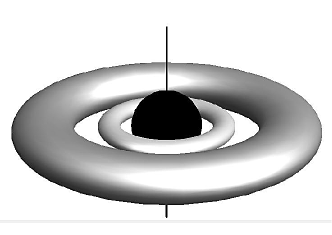
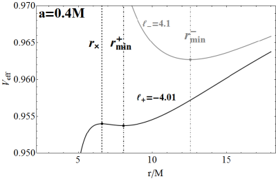
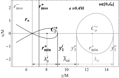
Figure 3: Upper: Pictorial representation of a doubled accretion toroidal systems orbiting a central Kerr black hole (black region)–see also in Fig. (4). Below: $\ell$counterrotating couple of accretion disks orbiting a central Kerr black hole attractor with spin $a=0.4M$. Effective potentials (left-panel), and cross sections on the equatorial plane of the outer Roche lobes (right-panel) for a couple $(\mathrm{C}_{i}^{+},\mathrm{C}_{o}^{-})$ made by an inner counterrotating disk and outer corotating disk corresponding to scheme III of Fig. (4). $(x,y)$ are Cartesian coordinates and $r_{\mathrm{mso}}^{\pm}$ are the marginally stable circular orbits for counterrotating and corotating matter respectively, $r_{\min}^{\pm}$ are the center of the outer Roche lobe (point of minimum of the fluid effective potentials): $(y_{3},y_{o})$ is in general the disk inner and the outer torus edge respectively, $\lambda_{o}=y_{1}^{o}-y_{3}^{o}$ is the elongation of the outer disk on the equatorial plane, $\lambda^{i}_{\times}$ is the elongation of the inner accreting disk, $\bar{\lambda}_{oi}$ is the spacing between the disks. Accretion for this couple (from the $r_{\times}$ point) may emerge only from the inner disk–Sec. (3.2.1).

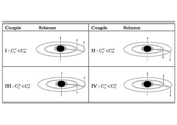
Figure 4: Pictorial schemes of a double system of accretion disks (gray thin rings) orbiting a Kerr black hole attractor. A ringed accretion disk of the order $n=2$ in the four principal states: black region is the black hole, gray region is the ergosphere. The distances between the disk and attractor are not in scale. The rings, $\mathrm{C}_{i}$ for the inner and $\mathrm{C}_{o}$ for the outer, are schematically represented as two-dimensional objects correspondent to the equilibrium topology. The arrows represent the rotation: the dimensionless spin of the attractor $a/M\geq 0$ is considered always positive, “spin-up” in the picture, or vanishing for the limiting case of the static Schwarzschild solution. The fluid specific angular momentum of an accretion disk $\ell$ can be positive, $\ell a>0$, for corotating $(-)$ (“spin-up”) or negative, $\ell a<0$, for counterrotating $(+)$ (“spin-down”) with respect to the central black hole. Rings are $\ell$corotating if $\ell_{i}\ell_{o}>0$ (scheme I and II-see also Figs (7)) or $\ell$counterrotating if $\ell_{i}\ell_{o}<0$ (scheme III and IV-see also Figs (3) and (11) respectively). A pictorial representation of this system can be found in Fig. (3)

We can introduce elongation $\Lambda_{\mathbf{C}^{2}}$ of $\mathbf{C}^{2}:\;\mathrm{C}_{a}<\mathrm{C}_{b}$ and the spacing $\bar{\Lambda}_{2,1}\equiv[y_{1}^{a},y_{3}^{b}]$ by the relations

$$\Lambda_{\mathbf{C}^{2}}\equiv[y_{3}^{a},y_{1}^{b}]=\left(\bigcup_{i=1}^{2}{\Lambda}_{i}\right)+\bar{\Lambda}_{2,1},\quad\lambda_{\mathbf{C}^{2}}\equiv y_{1}^{b}-y_{3}^{a}=\sum_{i}^{2}\lambda_{i}+\bar{\lambda}_{2,1}\geq\lambda_{\mathbf{C}^{2}}^{inf}\equiv\left.\sum_{i}^{2}\lambda_{i}\right|_{\sum_{i}\lambda_{i}},$$ (7)

where $\bar{\Lambda}_{i}$ and ${\Lambda}_{i}$ are the spacing and elongation of each ring and $\lambda_{\mathbf{C}^{2}}$ is the measure of the elongation of the (separated) configuration $\mathbf{C}^{2}$–see Fig. (3). Equation (7) shows that the minimum value $\lambda_{\mathbf{C}^{2}}^{inf}$ of the elongation $\lambda_{\mathbf{C}^{2}}$ is achieved, at fixed $\sum_{i}^{n}\lambda_{i}$, when $\bar{\lambda}_{2,1}=0$ that is for a $\mathbf{C}^{2}_{\odot}$ configuration of rank $\mathfrak{r}=\mathfrak{r}_{\max}$. As demostrated in Pugliese&Stuchlík (2015), we can introduce the effective potential $\left.V_{eff}^{\mathbf{C}^{2}}\right|_{K_{i}}$ of the decomposed $\mathbf{C}^{n}$ macro-structure and the effective potential $V_{eff}^{\mathbf{C}^{2}}$ of the configuration:

$$\left.V_{eff}^{\mathbf{C}^{2}}\right|_{K_{i}}\equiv V_{eff}^{1}\Theta(-K_{1})\bigcup V_{eff}^{2}\Theta(-K_{2})\quad\mbox{and}\quad V_{eff}^{\mathbf{C}^{2}}\equiv V_{eff}^{i}(\ell_{i})\Theta(r_{\min}^{o}-r)\Theta(r-r_{+})\bigcup V_{eff}^{o}(\ell_{o})\Theta(r-r_{\min}^{i}),$$ (8)

where $\Theta(-K_{i})$ is the Heaviside (step) function such that $\Theta(-K_{i})=1$ for $V_{eff}^{i}<K_{i}$ and $\Theta(-K_{i})=0$ for $V_{eff}^{i}>K_{i}$, so that the curve $V_{eff}^{\mathbf{C}}(r)$ is the union of all curves $V_{eff}^{i}(r)<K_{i}$ of its decomposition. Potential $\left.V_{eff}^{\mathbf{C}^{2}}\right|_{K_{i}}$ regulates behavior of each ring, taking into account the gravitational effects induced by the background, and the centrifugal effect induced by the motion of the fluid, while the potential $V_{eff}^{\mathbf{C}^{2}}$ governs the individual configurations considered as part of the macro-configuration–Fig. (3). Details on the effective potential, definition of differential rotation of the decomposition, specific angular momentum of the ringed disk and also for the thickness on the ringed disk can be found in Pugliese&Stuchlík (2015), where these configurations were first introduced, and then detailed in Pugliese&Stuchlík (2016a) for a configuration order $n\geq 2$. Here, we specialize the introduced concepts to the case of only two rings. In Sec. (3) we characterize the double accretion disk system, focusing in Sec. (3.1) on the $\ell$corotating couples, while in Sec. (3.2) we discuss the case of $\ell$counterrotating couples.

To simplify and illustrate the discussion, we use special graphs representing a couple of accretion disks and their evolution within the constraints they are subjected to. The case of a couple of tori orbiting around a single central Kerr black hole involves in general a remarkably large number of possible configurations: for a couple with fixed and equal critical topology, there could be $n=8$ different states according to their rotation and relative position of the centers. The couple $({\mathrm{C}_{\times},\mathrm{O}_{\times}})$, with different but fixed topology, could be in $n=16$ different states, while for the state $\mathrm{C}_{i}-{\footnotesize\textbf{()}}_{\times}$, with one equilibrium topology, we need to address $n=48$ different cases–see Figs. (5) for a sample of cases.

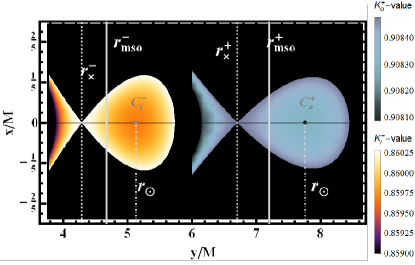
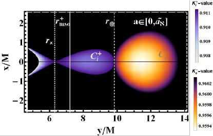
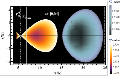
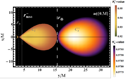
Figure 5: Density plot. Upper left: The $\ell$counterrotating colliding couple $\mathrm{C}_{\times}^{-}<\mathrm{C}_{\times}^{+}$, where $\ell_{+}=-3.99$, $\ell_{-}=3.31$ and $a=0.3825M$. Integration has been truncated prior collision. Upper right: $\ell$counterrotating couple $\mathrm{C}_{\times}^{+}<\mathrm{C}^{-}$, the contact point $r_{\otimes}$ is also signed where $a=0.385M$, $\ell_{-}=4.1$ and $\ell_{+}=-4.01$. Bottom left : $\ell$counterrotating couple $\mathrm{C}_{\times}^{+}<\mathrm{C}^{+}$, where $a=0.3M$, $\ell_{i}=-4.01$, $\ell_{o}=-4.9$. Bottom right : Colliding $\ell$corotating tori, $\mathrm{C}_{\times}^{-}<\mathrm{C}^{-}$, where $a=0.5M$, $\ell_{o}=5$, $\ell_{i}=3.3$. $(x,y)$ are Cartesian coordinates.

The use of graphic schemes is crucial for the representation of these cases, to quickly collect the different constraints on the existence and evolution of the states and for reference in our discussion. Therefore, although the following analysis is quite independent from the graph formalism, for easy reference, we include here a brief description of this formalism and discussion on the graph construction, introducing the essential blocks composing the graphs used in this work, and the list of notations and basic concepts related to these structures. We refer to Sec. (A) for details on the construction and interpretation of graphs associated with these systems, while in Fig. (6) we present the main blocks the graphs are made of, with a brief description which provides also a list of the main notation and definitions used throughout this work.

List of principal notation in the graph construction with reference to Fig. (6).

A graph vertex represents one configuration of the couple of tori as defined by the ringed disk topology and fluid rotation with respect to the central Kerr black hole attractor; then a vertex stands for one configuration of the set ${\footnotesize\textbf{()}}^{\pm}=\{\mathrm{C}^{\pm},\mathrm{C}^{\pm}_{\times},\mathrm{O}^{\pm}_{\times}\}$. The State lines connect two vertexes of the graph and represent a fixed couple of accretion tori disks. A monochromatic graph has one monochromatic state i.e. a state line connecting two $\ell$corotating configurations. A bichromatic graph has one bichromatic states i.e a state line connecting two $\ell$counterrotating configurations. For configuration sequentiality, signed on a state line and associated with the notation $\mathbf{<}$ or $\mathbf{>}$, we intend the ordered sequence of maximum points of the pressure, or $r_{\min}$, minimum of the effective potential which corresponds to the configuration centers. Therefore, in relation to a couple of rings, the terms “internal” (inner-$i$) or “external” (outer-$o$), will always refer, unless otherwise specified, to the sequence ordered according to the center location. For critical sequentiality, attached to a state line and associated with symbols $\mathbf{\succ}$ and $\mathbf{\prec}$, we refer to the sequentiality according to the location of the minimum points of the pressure, or $r_{\max}$, maximum point of the effective potential (in $\mathbf{L1}$ or $\mathbf{L2}$). A state line is completely oriented if both the configuration and critical sequentiality are specified, when the last one may be defined. Two configurations are correlated if they can be in contact, which implies collision in accordance with the constraints. In some cases there are particularly restrictive conditions to be satisfied for a correlation to occur (constrained non correlation). The addition of specific information on the lines and vertices of the graph, for example, the color the correlation and sequentiality is called graph decoration. An evolutive line connects two vertexes of two different state lines of the graph, and it represents the evolution of one configuration from one (starting) topology (vertex) to another topology (a vertex of a different state), for example from a $\mathrm{C}$ configuration to a $\mathrm{C}_{\times}$ in accretion. Evolutive lines may be composed to be closed on an initial vertex of the initial state lines creating a loop–Sec. (A.1). A central state of the graph is the couple, the graph configurations describes the evolution towards different states (every evolutive lines starts, ends or passes trough the central state). In this work the central state is the initial state line according to the evolution signed by the evolutive lines. Further details can be found in Sec. (A). State lines for $\ell$corotating couple are listed in Fig. (13) and state lines for $\ell$counterrotating couples are in Fig. (14). Fig. (8) describes monochromatic graphs while Fig. (9) exploit the bichromatic graphs.

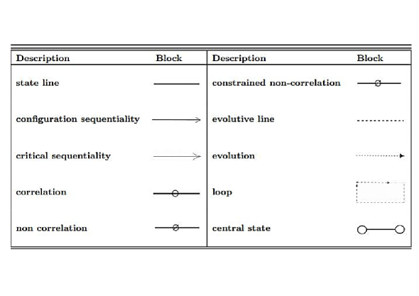
Figure 6: Graphs construction. Main blocks used in graphs of Figs (8) and (9)–see Sec. (2). Further details can be found in Sec. (A).

3 Characterization of the double tori disk system

In this Section we discuss the existence and the stability of the ringed disk $\mathbf{C}^{2}$ of the order $n=2$, made up by two toroidal configurations orbiting a spinning black hole attractor.

We first consider all the possible states for the couple of accretion disks with fixed topology. In the graph formalism their analysis is representing research of all the possible state and evolutive lines and their decoration (see Fig. (6) and end of Sec. (2)) according to the separation constraint. We refer to Sec. (A) for details on the construction and interpretation of graphs associated with these systems.

We shall prove that some states, or some decorations for a state are prohibited by several conditions, determined mainly by the dimensionless spin of the attractor and by the separation constraint. Specifically, we discuss the evolution of the configurations towards the phase of accretion onto the attractor which could lead to violate the separation condition. We study the collisions between the rings of the couple setting the emergence of the $\mathbf{C}_{\odot}^{2}$ (critical) macro-configuration, causing eventually the rings merging.

The states could be further constrained by the maximum possible extension of the closed configurations for fixed angular momentum, defined by the supremum of parameter $K$, $\sup{K}$. It is clear that for the $\mathrm{C}_{1}$ configurations we should consider the maximum of the elongation at the accretion $\lambda_{\times}$ and for the $\mathrm{C}_{2}$ disks the superior for $K_{\max}=1$. On the other hand, there is no similar constraint for the $\mathrm{C}_{3}$ configurations since there are no minimum points of the hydrostatic pressure. However, we can infer the presence of the constraints in terms of the location of the inner and outer edge of the torus with respect to the notable radii by considering the results of Pugliese&Stuchlík (2016a).

In Sec. (3.1), we will show how a monochromatic graph, generally describing the situation for a $\ell$corotating couple in any Kerr spacetime with $a\in[0,M]$ also describes the states and the evolution of a $\ell$counterrotating couple orbiting a Schwarzschild attractor ($a=0$), due to the particular geodesic structure of this static spacetime. Fig. (13) shows the possible state lines for the $\ell$corotating couples, while the possible state lines for the $\ell$counterrotating couples in a Kerr spacetime are listed in Fig. (14). Table (2) also provides guidance on the sequentiality of the $\ell$counterrotating couples according to criticality and the configuration order. The decorations of state lines show generally the emergence of possible collisions in accordance with the criteria used in the construction of the table, the location of the tori and the possible relation between the critical points.

Restricting our study to $\mathbf{C}^{2}$ configurations, we concentrate our attention onto the classification of the configurations with specific angular momenta $\ell\in\mathbf{Li}$ with $i\in\{1,2\}$–Pugliese&Stuchlík (2015). Some of these ringed disks are constrained to a configuration order $n_{\max}=2$.

1. The configuration:

   $$\bar{\mathfrak{C}}_{0}:\;\Delta_{cri}^{i}\cap\Delta_{cri}^{o}=\emptyset,\quad\mbox{there is}\quad a\neq 0,\;\ell_{i}\ell_{o}<0,\;{\footnotesize\textbf{()}}_{i}^{-}<{\footnotesize\textbf{()}}_{o}^{+}\quad\mbox{with}\quad{\footnotesize\textbf{()}}_{i}^{-}\prec{\footnotesize\textbf{()}}_{o}^{+},\quad n_{\max}(\bar{\mathfrak{C}}_{0})=2,$$ (9)

   and we have:

   $$-\ell^{o}_{+}\in]-\ell_{\mathrm{mso}}^{+},-\ell_{+}(r_{\mathrm{mso}}^{-})[\quad\mbox{and}\quad\ell^{i}_{-}\in]\ell_{\mathrm{mso}}^{-},\ell_{-}(r_{\mathrm{mso}}^{+})[.$$ (10)

   $$\mbox{For }a\in]0,a_{\aleph_{1}}[:\quad{\footnotesize\textbf{()}}_{o}^{+}\neq\mathrm{O}_{\times}^{+}\quad\mbox{for}\quad r_{\mathrm{mbo}}^{+}<r_{\mathrm{mso}}^{-}\quad\mbox{where}\quad a_{\aleph_{1}}:\;r_{\mathrm{mbo}}^{+}=r_{\mathrm{mso}}^{-}.$$ (11)

   Table (1) lists and summarizes the main features of the spin values singled out by analysis.

   Eq. (10) is fulfilled for the following topologies: at $a<\tilde{a}_{\aleph}$ for ${\footnotesize\textbf{()}}^{-}={\footnotesize\textbf{()}}_{1}^{-}$ and at $a<a_{\iota_{a}}<\tilde{a}_{\aleph}$ there could be only ${\footnotesize\textbf{()}}_{1}^{-}<{\footnotesize\textbf{()}}_{1}^{+}$–Fig. (9). Then, in $[a_{\iota_{a}},\tilde{a}_{\aleph}]$, there is ${\footnotesize\textbf{()}}_{1}^{-}<{\footnotesize\textbf{()}}_{2}^{+}$ and ${\footnotesize\textbf{()}}_{1}^{-}<{\footnotesize\textbf{()}}_{1}^{+}$. Whereas at $a\in[\tilde{a}_{\aleph},a_{\gamma_{+}}^{-}]$ there is also ${\footnotesize\textbf{()}}_{2}^{-}<{\footnotesize\textbf{()}}_{2}^{+}$, and in $[a_{\gamma_{+}}^{-},\breve{a}_{\aleph}]$ there is also ${\footnotesize\textbf{()}}_{2}^{-}<{\footnotesize\textbf{()}}_{3}^{+}$. Finally for $a>\breve{a}_{\aleph}$ also the couple ${\footnotesize\textbf{()}}^{-}_{3}<{\footnotesize\textbf{()}}_{3}^{+}$ is possible. These constraints, however, are not sufficient to fully characterize the couples ${\footnotesize\textbf{()}}^{-}<{\footnotesize\textbf{()}}^{+}$ as discussed in Sec. (3.2.2), in fact not all the couples ${\footnotesize\textbf{()}}^{-}<{\footnotesize\textbf{()}}^{+}$ belong to the $\bar{\mathfrak{C}}_{0}$ class.

   Table 1: Classes of attractors. In general given a spin value $a_{\bullet}$ the classes $\mathbf{A}_{\bullet}^{\lessgtr}$ stands for the ranges $a\in[0,a_{\bullet}[$ and $a\in]a_{\bullet},M]$ respectively. Some of these classes are given alongside the spins.

   Spins and classes of attractors
   ${a_{\aleph_{2}}}\equiv 0.172564M:-\ell_{\mathrm{mso}}^{+}=\ell_{\mathrm{mbo}}^{-}$	${a_{\iota}}\equiv 0.3137M:r_{\mathrm{mbo}}^{-}=r_{\gamma}^{+}$-$\left({\mathbf{A}}_{\iota}^{\lessgtr}\right)$	${a_{\iota_{a}}}\equiv 0.372583M:r_{\mathrm{mso}}^{-}=r_{\mathrm{mbo}}^{+}$ -$\left(\mathbf{A}_{\iota_{a}}^{\lessgtr}\right)$
   $a_{\aleph_{1}}=0.382542M:\ell_{\gamma}^{-}=-\ell_{+}\left(r_{\mathrm{mso}}^{-}\right)$	${a_{\aleph_{0}}}\equiv 0.390781M:\ell_{\gamma}^{-}=-\ell_{\mathrm{mbo}}^{+}$	${\tilde{a}_{\aleph}}\approx 0.461854M:\ell_{-}(r_{\mathrm{mso}}^{+})=\ell_{\mathrm{mbo}}^{-}$
   $a_{{}_{u}}=0.474033M:\;\bar{\mathfrak{r}}_{\mathrm{mbo}}^{+}=\bar{\mathfrak{r}}_{\gamma}^{-}$	${a_{\aleph}}\approx 0.5089M:-\ell_{\mathrm{mso}}^{+}=\ell_{\gamma}^{-}$	${a_{\gamma_{+}}^{-}}\equiv 0.638285M:r_{\gamma}^{+}=r_{\mathrm{mso}}^{-}$
   ${{a}_{1}}\approx 0.707107M:r_{\gamma}^{-}=r_{\epsilon}^{+}$	${\breve{a}_{\aleph}}=0.73688M:\ell_{-}(r_{\mathrm{mso}}^{+})=\ell_{\gamma}^{-}$	${{a}_{b}}\approx 0.828427M:r_{\mathrm{mbo}}^{-}=r_{\epsilon}^{+}$
   ${a_{\mathcal{M}}^{-}}\equiv 0.934313M:\ell_{\gamma}^{-}=\ell_{\mathcal{M}}^{-}$	${a_{2}}\approx 0.942809M:r_{\mathrm{mso}}^{-}=r_{\epsilon}^{+}$	${\breve{a}}\equiv 0.969174M:\breve{\ell}^{-}=r_{\gamma}^{-}$ $\left(\mathbf{\breve{A}_{\lessgtr}}\right)$

2. The configuration:

   $$\bar{\mathfrak{C}}_{1a}: \;r_{\max}^{o}\in\Delta_{crit}^{i},\quad\mbox{thus}\quad\ell_{i}\ell_{o}<0\quad{\footnotesize\textbf{()}}_{i}^{-}\lessgtr{\footnotesize\textbf{()}}_{o}^{+}\quad{\footnotesize\textbf{()}}_{o}=!\mathrm{C}_{o}\quad n_{\max}(\bar{\mathfrak{C}}_{1a})=2$$ (14)

   $$\mbox{if}\quad{\footnotesize\textbf{()}}_{o}^{-}<{\footnotesize\textbf{()}}_{o}^{+}:\quad\mbox{then}\quad{\footnotesize\textbf{()}}_{i}^{-}\prec{\footnotesize\textbf{()}}_{o}^{+}\quad{\footnotesize\textbf{()}}_{o}^{+}=!\mathrm{C}^{+}\quad n_{\max}(\bar{\mathfrak{C}}_{1a})=2$$

   $$\mbox{if}\quad{\footnotesize\textbf{()}}_{i}^{+}<{\footnotesize\textbf{()}}_{o}^{-}:\quad\mbox{then}\quad{\footnotesize\textbf{()}}_{o}^{-}=!\mathrm{C}^{-}\quad{\footnotesize\textbf{()}}_{i}^{+}\prec{\footnotesize\textbf{()}}_{o}^{-}:\quad(a\gtrapprox 0).$$

   Here, for any relation $\mathbf{\Large{\bowtie}}$ among two quantities, in $\bowtie!$ the intensifier $(!)$ a reinforcement of the relation, indicates that this is a necessary relation which is always satisfied.

3. The configuration:

   $$\bar{\mathfrak{C}}_{1b}:\quad\Delta_{crit}^{i}\subset\Delta_{crit}^{o}\quad\mbox{then there is }\ell_{i}\ell_{o}\lessgtr 0\quad{{\textbf{{\footnotesize{()}}}}}_{i}<{\footnotesize\textbf{()}}_{o}\quad{\footnotesize\textbf{()}}_{i}\succ{\footnotesize\textbf{()}}_{o}\quad{\footnotesize\textbf{()}}_{o}=!\mathrm{C}_{o}\quad n_{\max}(\bar{\mathfrak{C}}_{1b})=\infty.$$ (15)

   A special case of this class of ringed disks are the couples $\ell_{(i+1)/i}=-1$, which can have $\ell_{-}/-\ell_{+}\gtrless 1$.

We finally note that, in a Kerr spacetime $(a\neq 0)$, the chromaticity of the graphs is determined by the relative rotation of the disks together with the rotation with respect to the attractor, however the situation is different in the case of static limit for the attractor with $a=0$, where monochromatic graphs describe also $\ell$counterrotating (i.e. $\ell_{i}\ell_{o}<0$) (and $\ell$corotating $\ell_{i}\ell_{o}>0$) couples. In fact, in the case of a Schwarzschild attractor (static spacetime), it is still possible to consider a bichromatic graph with an arbitrary choice of tori relative rotation $\ell_{i}\ell_{j}<0$, but the spacetime geodesic structure is singled out by the properties of the Schwarzschild geometry, independently of the sign of the fluid angular momentum. Therefore at all the effects this bichromatic graph must undergo the analysis on the monochromatic graph. However, a major difference between a bichromatic graph where $a=0$ and the monochromatic one occurs in the static spacetime for the $\ell$counterrotating case due to the possible evolutive loops of the bichromatic vertices, where collision between tori with $\ell$counterrotating angular momentum may occur. In the following Sec. (3.1) we specialize the discussion for the Schwarzschild geometry and the $\ell$corotating couples in the Kerr spacetimes, while the $\ell$counterrotating couples orbiting a Kerr attractor are analysed in Sec. (3.2).

3.1 The $\ell$corotating couples in the Kerr spacetime and the case of the Schwarzschild geometry

Two $\ell$corotating tori must have different specific angular momentum, i.e., $\ell_{o}/\ell_{i}\equiv\ell_{o/i}>1$. They have to be both corotating or counterrotating with respect to the central black hole, as in scheme I and II of Fig. (4).

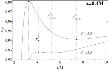
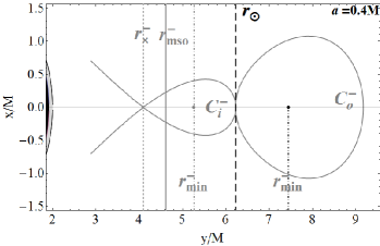
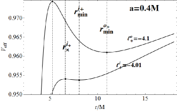
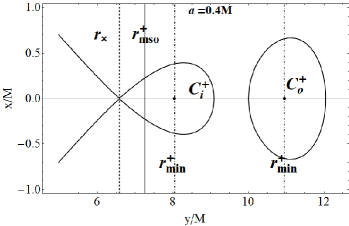
Figure 7: $\ell$corotating couples of accretion disk orbiting a central Kerr black hole attractor with spin $a=0.4M$. Effective potentials (left-panels), and cross sections on the equatorial plane of the outer Roche lobes for a couple of counterrotating disks $(\mathrm{C}_{i}^{+},\mathrm{C}_{o}^{+})$ (right-below), and corotating disks $(\mathrm{C}_{i}^{-},\mathrm{C}_{o}^{-})$ (right-upper), correspond to scheme I and II of Fig. (4) respectively. $(x,y)$ are Cartesian coordinates and $r_{\mathrm{mso}}^{\pm}$ are the marginally stable circular orbits for counterrotating and corotating matter respectively Accretion for an $\ell$corotating couple (from the $r_{\times}$ point) may emerge only from the inner disk. Collision (at contact point $r_{\odot}$) between the outer Roche lobes of the disks, here shown for the couple $(\mathrm{C}_{i}^{-},\mathrm{C}_{o}^{-})$ (upper), is possible for any $\ell$corotating couples–see also Fig. (8).

We will always intend relations between the magnitude of the specific angular momentum, if not otherwise specified. However, we should consider that for the corotating fluids there could occur the penetration of the geodesic corotating structure into the ergoregion, which does not occur for the counterrotating rings, and by the different behaviour $\partial_{a/M}r_{\mathrm{N}}^{\pm}\gtrless 0$ and $\partial_{a/M}\bar{\mathfrak{r}}_{\mathrm{N}}^{\pm}\gtrless 0$ –see Figs (1) and Figs (2).

In terms of the graph models, introduced in Fig. (6) and Sec. (2), the $\ell$corotating couples are represented by monochromatic graph of Fig. (8).

We set up our analysis by considering an initial state of equilibrium, formed by a couple of tori in equilibrium. The possible (initial or final) states for this case are listed in Fig. (13). This state represents also the graph center in Fig. (8), which have therefore only a subsequent section or loops. Except the case of evolutive loops, in general we will deal with a system which is evolving from an initial state of equilibrium towards unstable configurations. In other words, for convenience of discussion we adopt here the arbitrary assumption of existence of a phase in the formation of the double tori system in which both tori are in an equilibrium state, and the system can eventually evolve towards an instability phase $\mathbf{C_{\times}}^{2}$, $\mathbf{C_{\odot}}^{2}$ or also $\mathbf{C_{\odot}^{\times}{}^{2}}$. It is easy to see that choice of a different initial state and therefore a different graph center does not change qualitatively the graph which will be just centered in a different state.

We start our analysis of the couple by focusing on the state lines representing all possible couples of disks orbiting a Kerr attractor with dimensionless spin $a/M\in[0,1]$, according to the constraints imposed by the geodesic structure and the condition of non-penetration of matter. Then we discuss the system evolution connecting, whenever possible, the different state lines with the evolutive lines. Graphs construction in the $\ell$corotating case is detailed in Sec. (A). We discuss the possible evolutive loop for the $\ell$corotating couples and the $\ell$counterrotating couples in the static spacetimes in Sec. (A.1). State lines, represented here in Fig. (13), were introduced in Pugliese&Stuchlík (2016a). We here report the principal results adapted to the case of ringed disks of the order $n=2$–see also Pugliese&Stuchlík (2016c).

Couple evolution from equilibrium to instability

We start our considerations by assuming that the initial state for a tori pair provides two equilibrium topologies, $\mathrm{C}_{i}<\mathrm{C}_{o}$, then we shall consider possible evolution towards an instability or a sub-configuration ${\footnotesize\textbf{()}}_{\times}$ of the pair, and possible collision, where the emergence of configurations $\mathbf{C}_{\oplus}^{2}$ will be deepened in Sec. (3.3).

Considering the no loop evolution, a couple of tori in a Schwarzschild spacetime and the $\ell$corotating systems around a Kerr geometry are completely described by the graph in Fig. (8).

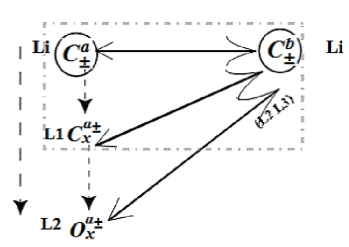
Figure 8: $\ell$corotating couples corresponding to scheme I and II of Fig. (4) see also Figs (7). Evolutive graph of a double accretion disk system made by a couple of $\ell$corotating toroidal disks (monochromatic graph). This case also describes an $\ell$counterrotating couple of toroidal disks (bichromatic graph) in a static spacetime $(a=0)$. The initial state is assumed to be the couple of configuration in equilibrium ${\footnotesize\textbf{()}}_{\pm}-{\footnotesize\textbf{()}}_{\pm}$. Description of graph blocks are in Fig. (6). State lines for $\ell$corotating couple are listed in Fig. (13)–see Sec. (3.1).

In any monochromatic graph (or bichromatic graph in a static spacetime), all the state lines are oriented in the same direction–Fig. (8). Because of assumptions of the unique geodesic structure of the background geometry, there is no evolutive phase in which the outer disk of the couple is accreting, but only the inner configuration of the doubled system can accrete onto the source. Only the inner disk of the couple could evolve towards the unstable topology, and the subsequent section is formed by the evolutions of the inner vertex only. The evolution of the final state, due to the inner vertex, can affect all the state lines and their evolutions. Two tori, which are both corotating or counterrotating with respect to the central attractor, can admit only the inner configuration accreting and if, for some processes, the outer accretion disk would approach its unstable phase, then the double ($\ell$corotating) system would be destroyed for collision or merging before the outer ring would effectively reach its unstable topology. This reduces the possibility of existence of the double tori system and its stability–as shown in Pugliese&Stuchlík (2016c) the possible states with an instability are $\mathrm{C}^{\pm}_{\times}<\mathrm{C}^{\pm}$ for $a\in[0,M]$ (and $\mathrm{C}^{\pm}_{\times}<\mathrm{C}^{\mp}$ for $a=0$). This is property of any couple of $\ell$corotating tori regardless the dimensionless spin of the attractor and largely also of a single accretion disk model, as long as it is assumed that the accretion occurs at the (stressing) inner margin of the disk which is located at $r_{in}\in]r_{\mathrm{mbo}},r_{\mathrm{mso}}]$. Therefore the outer ring have to be considered to be quiescent–i.e. in equilibrium . It can however grow, increasing the $K$ parameter, or it can change the specific angular momentum. Thus also changes in the ring morphology may cause an instability of the entire ringed disk for ring collision. Moreover, even with a quiescent outer ring, an accretion phase occurring in the inner ring could induce a ring collision, during the earliest stage of the accretion, the inner ring reaches, according to its specific angular momentum, its maximal elongation on the equatorial plane, i.e. $\lambda_{i}=\lambda_{\times}^{i}=\max{\lambda}$ where $K=K_{\max}$, and the inner disk outer margin moves outwardly. On the other hand, the outer ring could collide with the inner one, and eventually merging with this leading to an accretion or inducing an evolutive loop. Therefore, we need to discuss these two different, competitive phenomena for accretion of the inner ring and collision among the rings and the subsequent three fates this may induce. It is therefore interesting to discuss the emergence of loops for monochromatic graphic and the possibility of merging of tori– see Sec. (A.1).

3.2 The $\ell$counterrotating couples

We consider the $\ell$counterrotating couples orbiting a Kerr attractor with dimensionless spin $a/M\in]0,1]$ corresponding to bichromatic graphs–see schemes III and IV of Fig. (4). In comparison to $\ell$corotating couples (monochromatic graph), or $\ell$counterrotating torii orbiting a Schwarzschild black hole, this case is complex, being diversified for classes of attractors, and for the disk spin orientation with respect to the central attractor–Pugliese&Stuchlík (2016a). It is therefore necessary to consider separately the case $\mathrm{C}^{+}<\mathrm{C}^{-}$ (inner counterrotating torus and outer corotating torus), discussed in Sec. (3.2.1) from the $\mathrm{C}^{-}<\mathrm{C}^{+}$ case (inner corotating ring and outer counterrotating torus), investigated in Sec. (3.2.2). The graph formalism can significantly simplify the analysis of the evolution of this particular double system. Using the results of Pugliese&Stuchlík (2016a) we build the Fig. (14) collecting the main states for the graph in Fig. (9).

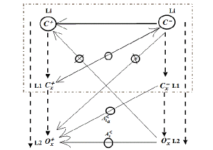
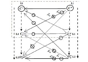
Figure 9: Graph of a double $\ell$counterrotating tori in a Kerr black hole spacetime $a\in]0,M[$ (bichromatic graph). Left: graph centered in the initial state $\mathrm{C}^{+}<\mathrm{C}^{-}$–see also scheme III of Fig. (4) and Fig. (3). Right: graph centered in the initial state $\mathrm{C}^{-}<\mathrm{C}^{+}$–see also scheme IV of Fig. (4) and Figs (11). The initial state is assumed to be the couple of configuration in equilibrium. Description of graph blocks is in Fig. (6). State lines for $\ell$counterrotating couples are in Fig. (14).

The most relevant effect distinguishing these pairs from the $\ell$corotating couples is that the (counterrotating) outer torus of the couple in general may undergo a P-W instability phase with the emergence of an instability point eventually giving rise to a feeding of material towards its companion inner torus.

The double sequentiality according to the configuration and criticality indices, respectively, of some lines of Table  (14) and the states of Fig. (9) are not specified, depending on the vertex decoration in terms of the angular momentum. In fact, as demonstrated in Pugliese&Stuchlík (2015, 2016a), the sequentiality of centers of the $\ell$counterrotating couples in equilibrium does not necessarily constrain the critical sequentiality ($\ell{\LARGE{\not}}{\in}\mathbf{L3}$): there are special cases where, at fixed $\ell_{i}\ell_{o}<0$, with ${\footnotesize\textbf{()}}_{i}<{\footnotesize\textbf{()}}_{o}$, there can be ${\footnotesize\textbf{()}}_{i}\prec{\footnotesize\textbf{()}}_{o}$, which corresponds to $\bar{\mathfrak{C}}_{0}$ in Eq. (9) (if there is $\mathrm{C}^{-}<\mathrm{C}^{+}$), or otherwise it corresponds to $\bar{\mathfrak{C_{1_{a}}}}$ in Eq. (14) within the conditions Eq. (14) or (14), or, conversely, there can be ${\footnotesize\textbf{()}}_{i}\succ{\footnotesize\textbf{()}}_{o}$ i.e. a couple of the $\bar{\mathfrak{C_{1_{b}}}}$ class, in Eq. (15), which includes also the $\ell$corotating couples.

Then the outer vertex of the $\bar{\mathfrak{C_{1_{a}}}}$ and $\bar{\mathfrak{C_{1_{b}}}}$ couples must be in equilibrium or destroyed: this means that before the outer torus reaches its unstable phase the ringed disk will be destroyed for collision, prohibiting any subsequent evolutive lines.

Such a situation may be prevented if a change of criticality order occurs, which means a transition from a $\bar{\mathfrak{C_{1_{a}}}}$ or $\bar{\mathfrak{C_{1_{b}}}}$ class to $\bar{\mathfrak{C_{0}}}$ class. However, as the inversion of the configuration sequentiality is not permitted, such a transition could happen only for the couples ${\footnotesize\textbf{()}}^{-}<{\footnotesize\textbf{()}}^{+}$, detailed in Sec. (3.2.2).

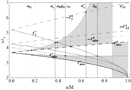
Figure 10: Fluid specific angular momentum $\ell^{\pm}_{i}=\ell^{\pm}(r^{\pm}_{i})$ where $r^{\pm}_{i}\in\{\mathbf{R}_{\mathrm{N}}^{\pm},r_{\mathcal{M}}^{\pm}\}$, $r_{\mathcal{M}}^{\pm}$ is the maximum point of derivative $\partial_{r}(\mp\ell^{\pm})$ for $a/M$ respectively and $\mathbf{R}_{\mathrm{N}}\equiv\{r_{\gamma}^{\pm},r_{\mathrm{mbo}}^{\pm},r_{\mathrm{mso}}^{\pm}\}$. Some notable spacetime spin-mass ratios are also plotted, a list can be found in Table (1). Dotted-dashed curves are respectively $-\ell^{+}(r_{mso}^{-})\geq\ell^{-}(r_{mso}^{+})$.

In fact, in the isolated disks–attractor systems, the couple evolution is strongly determined by the decoration of the initial state. However, conditions for occurrence of this class transition are very complex, depending on the relation between characteristic values of the specific angular momentum $\{\mp\ell_{\mathrm{mso}}^{\pm},\mp\ell^{\pm}(r_{\mathrm{mso}}^{\mp})\}$ which determine the boundaries of the ranges in Eq. (10)–see also Fig. (1).

More generally, for $\ell{\LARGE{\not}}{\in}\mathbf{L3}$ we can discuss the state sequentiality according to the arguments presented in Pugliese&Stuchlík (2015, 2016a). We distinguish two cases according to the magnitude of the specific angular momentum.

1. $$\mbox{For}\quad|\ell_{-}/\ell_{+}|>1\quad\mbox{ \emph{there must be }}\quad\bar{\mathfrak{C}}_{1b}\quad\mbox{of Eq.~{}(\ref{C1b})}\quad\mbox{or}\quad{\footnotesize\textbf{()}}^{+}<\mathrm{C}^{-}\quad\mbox{and}\quad{\footnotesize\textbf{()}}^{+}\succ\mathrm{C}^{-}.$$ (16)

   This case, analyzed in Sec. (3.2.1) and represented by the scheme III of Fig. (4), is described by the graph of Fig. (9)-left. As confirmed by the graph Fig. (9)-left, only the inner counterrotating ring can accrete onto the source. On the other hand, the condition ${\footnotesize\textbf{()}}^{+}<\mathrm{C}^{-}$ does not necessarily imply the relation of Eq. (16) for the angular momentum. Moreover, the condition ${\ell_{-}>-\ell_{\mathrm{mso}}^{+}}$ implies strong constraints on the initial state of the outer corotating torus of the couple. In fact, due to the constraint $|\ell_{-}/\ell_{+}|>1$, if the attractor belongs to the class $a<a_{\aleph_{2}}$ (where $a=a_{\aleph_{2}}:\;-\ell_{\mathrm{mso}}^{+}=\ell_{\mathrm{mbo}}^{-}$), the outer corotating torus can belong to one of the ranges $\mathbf{Li}$. For $a\in]a_{\aleph_{2}},a_{\aleph}[$, the outer corotating torus specific angular momentum has to be in $\mathbf{L2}$ or $\mathbf{L3}$, and for $a>a_{\mathcal{M}}$, the torus is centered at $r>r_{\mathcal{M}}^{-}$. For the faster attractors with $a>a_{\aleph}$ (at $a=a_{\aleph}:\;-\ell_{\mathrm{mso}}^{+}=\ell_{\gamma}^{-}$) the corotating torus has to be located far from the attractor, having the specific angular momentum in $\mathbf{L3}$; the corresponding effective potential has thus no maximum points–Fig. (1).

2. $$\mbox{For}\quad{|\ell_{-}/\ell_{+}|<1}\quad\mbox{there is }\quad{\footnotesize\textbf{()}}^{-}\lessgtr{\footnotesize\textbf{()}}^{+},\quad\mbox{and}\quad r_{\min}^{-}<\bar{\mathfrak{r}}\quad\mbox{ where }\bar{\mathfrak{r}}>r_{\mathrm{mso}}^{-}:\;\ell_{-}=-\ell_{+}>\ell_{\mathrm{mso}}^{+}$$ (17)

   $$\mbox{if}\quad\ell_{-}\in]\ell_{-}(r_{\min}^{+}),\ell_{-}(\bar{\mathfrak{r}})[\quad\mbox{then there is }\quad{\footnotesize\textbf{()}}^{+}<{\footnotesize\textbf{()}}^{-},$$ (18)

   $$\mbox{if}\quad\ell_{-}\in]\ell_{\mathrm{mso}}^{-},\ell_{-}(r_{\min}^{+})[\quad\mbox{then there is }\quad{\footnotesize\textbf{()}}^{-}<{\footnotesize\textbf{()}}^{+}.$$ (19)

   The sequentiality according to the criticality has been fixed in the first column of Table (2), combining the additional restrictions provided by the angular momentum and the constraints from the complementary geodesic structure of spacetime $\bar{\mathbf{R}}_{\mathrm{N}}$, represented in Fig. (1).

   The case ${\footnotesize\textbf{()}}^{+}<{\footnotesize\textbf{()}}^{-}$ of (18) is described in Fig. (9)-right and represented in scheme IV of Fig. (4), see also Fig. (3). We note that in general, a small range of angular momentum in the case ${\footnotesize\textbf{()}}^{+}<{\footnotesize\textbf{()}}^{-}$ with $|\ell_{-}/\ell_{+}|<1$, is associated to a limited orbital region which decreases as the torus distance from the attractor increases, or its dimensionless spin decreases, i.e., in the $R\equiv r/a\gg r_{\mathrm{mso}}/a$ limit. In fact this behavior could be interpreted as a consequence of the rotational effects of the attractor which disappear in the Newtonian limit. The existence of such a $\mathrm{C}^{-}>\mathrm{C}^{+}$ couple is very constrained since the extension of the orbital difference, $r_{\min}^{-}-r_{\min}^{+}$, in the case $\mathrm{C}^{-}>\mathrm{C}^{+}$ is very limited and depends on the $r_{\mathcal{M}}^{\pm}$; such toroidal configurations are more prepared to collide with subsequent possible merging of the tori.

   The case ${\footnotesize\textbf{()}}^{-}<{\footnotesize\textbf{()}}^{+}$ of (19) is shown in Fig. (9)-left and scheme III of Fig. (4)–see also Figs (11). The possible specific angular momentum of the $\mathrm{C}^{-}$ configuration with $\ell_{-}<-\ell_{+}$ (for $\mathrm{C}^{+}<\mathrm{C}^{-}$ or $\mathrm{C}^{-}<\mathrm{C}^{+}$) depends on the unstable topology of the ${\footnotesize\textbf{()}}^{+}$ torus. The instability of the ${\footnotesize\textbf{()}}^{+}<{\footnotesize\textbf{()}}^{-}$ couple must take place on ${\footnotesize\textbf{()}}^{+}$. When $\ell_{+}\in\mathbf{L1}$, then there is the maximum possible separation between the centers of the couple. Therefore, it is necessary to consider the angular momentum $\ell_{-}(r_{\min}^{+})$, which is the lower limit of the range in Eq. (18) and the specific angular momentum $\ell_{-}(\bar{\mathfrak{r}})=-\ell_{+}(r_{\min}^{+})$ which is the upper limit of this range. We can establish the upper-bound by considering the topology of the ${\footnotesize\textbf{()}}^{+}$ configuration and the constraints on the ranges of the angular momentum. Whereas, the lower bound satisfies the relation $\ell_{-}(r_{\min}^{+})<\ell_{-}<\ell_{-}(\bar{\mathfrak{r}})=-\ell_{+}(r_{\min}^{+})$–see Table (2) and Pugliese&Stuchlík (2016a). In fact, it is necessary to know the radius $r_{\min}^{+}$, for fixed range of $\ell_{+}$, and then establish the range of angular momentum $\ell_{-}$ of the corotating torus centered in $r_{\min}^{+}$–see also Pugliese&Stuchlík (2015). Then, we can combine the restrictions provided by the angular momentum range and those derived from the condition on the relation of the two angular momenta with results of Table (2). Therefore, having a $\mathrm{C}^{+}_{3}$ torus then the ${\footnotesize\textbf{()}}^{-}$ torus can be in any topology, analogously, but with some restrictions, for $\mathrm{C}^{+}_{2}$, mainly for $\mathrm{C}_{3}^{-}$ and $\mathrm{C}_{2}^{-}$ for slow attractors ($a<a_{\aleph_{0}}=0.390781M\;\ell_{\mathrm{mso}}^{+}=-\ell_{\mathrm{mbo}}^{-}$). For a $\mathrm{C}^{+}_{1}$ torus there is only $\mathrm{C}^{-}\neq\mathrm{C}_{3}^{-}$ for $a<a_{\aleph_{0}}$. If $\mathrm{C}^{-}=\mathrm{C}_{1}^{-}$ or $\mathrm{C}_{2}^{-}$, then $\mathrm{C}^{+}$ can be in any angular momentum range , but subjected to several restrictions if orbiting around slower attractors. However, these results have to be combined with those presented in Table (2). If $\mathrm{C}^{-}=\mathrm{C}^{-}_{2}$, we have only the constraints provided by the complementary geodesic structure given in Table (2), while if $\mathrm{C}^{-}=\mathrm{C}^{-}_{3}$ then, for $a<a_{\aleph_{0}}$, we have $\mathrm{C}^{+}=\mathrm{C}_{2}^{+}$ or $\mathrm{C}_{3}^{+}$.

Sec. (3.2.1) and Sec. (3.2.2), are dedicated to the $\ell$ounterrotating couples, focusing on the sequentiality. As conclusion on this analysis we summarize the situation in the following points:

1. $$\mbox{For}\quad{\footnotesize\textbf{()}}^{-}<{\footnotesize\textbf{()}}^{+}\quad\mbox{there is}\quad|\ell_{-}/\ell_{+}|<1\quad\mbox{and }\quad\ell_{-}\in]\ell_{\mathrm{mso}}^{-},\ell_{-}(r_{\min}^{+})[,$$ (20)

   see Sec. (3.2.2) and Eq. (19). This case is detailed in Sec. (B.0.2) where additional restrictions are discussed. The relation between the instability points (for $\ell{\LARGE{\not}}{\in}\mathbf{L3}$), which is the critical sequentiality, is fully addressed in Sec. (B.0.3) and Table (2).

   In fact, the angular momenta of the tori in ${\footnotesize\textbf{()}}^{-}<{\footnotesize\textbf{()}}^{+}$, are fixed in second-column of Table (2), while the location of the eventual instability points has been established in Fig. (14) and first-column of Table (2). Since the distance between the radii $r_{\mathrm{mso}}^{+}>r_{\mathrm{mso}}^{-}$ increases with increasing spin of the attractor, for some ranges of angular momentum the critical points of the outer counterrotating configuration are $r_{\mathrm{mso}}^{-}<r_{\max}^{+}<r_{\mathrm{mso}}^{+}$, and the couple of (20) are ${\footnotesize\textbf{()}}^{-}<{\footnotesize\textbf{()}}^{+}$ with ${\footnotesize\textbf{()}}^{-}\prec{\footnotesize\textbf{()}}^{+}$ as shown in Table (2). Therefore, this couple is a $\mathfrak{\bar{C}_{1_{a}}}$ one within the conditions of Eq. (14) for $r_{\mathrm{mso}}^{-}<r_{\max}^{+}<r_{\min}^{-}<r_{\min}^{+}$, or a $\mathfrak{\bar{C}_{0}}$ of Eq. (9) if $r_{\mathrm{mso}}^{-}<r_{\min}^{-}<r_{\max}^{+}<r_{\mathrm{mso}}<r_{\min}^{+}$. Therefore, the situation depends on the angular momentum of the outer configuration and the class of the attractor. On the other hand, if $r_{\max}^{+}<r_{\mathrm{mso}}^{-}$, then assuming $\tilde{\ell}_{-}\equiv\ell_{-}(r_{\max}^{+})\in]\ell_{\mathrm{mso}}^{-},\ell_{-}(r_{\min}^{+})[$ this angular momentum separates the configurations with $\ell_{-}\in]\ell_{\mathrm{mso}}^{-},\ell_{-}(r_{\max}^{+})[$ where $r_{\max}^{-}>r_{\max}^{+}$ implying ${\footnotesize\textbf{()}}^{-}<{\footnotesize\textbf{()}}^{+}$ with ${\footnotesize\textbf{()}}^{-}\succ{\footnotesize\textbf{()}}^{+}$ which is a $\bar{\mathfrak{C}}_{1b}$ of Eq. (15), from those with $\ell_{-}\in]\ell_{-}(r_{\max}^{+}),\ell_{-}(r_{\min}^{+})[$ where $r_{\max}^{-}<r_{\max}^{+}$ implying ${\footnotesize\textbf{()}}^{-}<{\footnotesize\textbf{()}}^{+}$ with ${\footnotesize\textbf{()}}^{-}\prec{\footnotesize\textbf{()}}^{+}$ which is a $\bar{\mathfrak{C}}_{1a}$ one of Eq. (14).

2. Conversely for the couple of tori

   $${\footnotesize\textbf{()}}^{-}>{\footnotesize\textbf{()}}^{+}\quad\mbox{ there is either}\quad$$ (21)

   $$\bar{\mathfrak{C}}_{1a}:\;\mathrm{C}^{-}>{\footnotesize\textbf{()}}^{+}\quad\mbox{and}\quad\mathrm{C}^{-}\succ{\footnotesize\textbf{()}}^{+}\quad\mbox{within conditions of Eq.~{}(\ref{Eq:so2}) or}$$

   $$\bar{\mathfrak{C}}_{1b}:\;\mathrm{C}^{-}>{\footnotesize\textbf{()}}^{+}\quad\mbox{and}\quad\mathrm{C}^{-}\prec{\footnotesize\textbf{()}}^{+}.$$

   $$\quad\mbox{There can be}\quad|\ell_{-}/\ell_{+}|>1\quad\mbox{if}\quad r_{\min}^{-}>\bar{\mathfrak{r}}_{-},\quad\mbox{then we obtain }\quad\bar{\mathfrak{C}}_{1b}\quad\mbox{according to Eq.~{}(\ref{Eq:fac-tus}), }$$

   $$\quad\mbox{or there is }\quad|\ell_{-}/\ell_{+}|<1\quad\mbox{if}\quad r_{\min}^{-}\in]r_{\min}^{+},\bar{\mathfrak{r}}_{-}[,\quad\mbox{where}\quad\bar{\mathfrak{r}}_{-}:\;\ell_{-}(\bar{\mathfrak{r}}_{-})=-\ell_{+}.$$

   The outer corotating torus of this couple cannot be unstable, as shown in Sec. (3.2.1).

Finally we conclude this section mentioning the couples with

$$\ell_{i/o}=-1\quad\mbox{which corresponds to the case}\quad\bar{\mathfrak{C}}_{1_{b}}\quad\mbox{considered in Eq.~{}(\ref{C1b})},$$ (22)

discussed also in Pugliese&Stuchlík (2015) as limiting cases for the perturbation analysis and as limiting situation of $|\ell_{i/o}|\lessgtr 1$.

The evolution of these systems is fully described in the graphs of Fig. (9). Comparing the graphs of Fig. (8) and Fig. (9), it is clear that in the $\ell$counterrotating case both vertices of a state may evolve. As a consequence of this a change of the central state of the graph (which is also the initial state, the graph having only a subsequent section) generally heavily deform the entire graph, being strongly dependent on the initial data (the decorations of the state vertices). The evolution of a state line is highly constrained by the initial decoration, as can be seen by comparing Fig. (13) for the $\ell$corotating states and Fig. (14) and Table (2) for the $\ell$counterrotating states. Consequently we have only a limited number of possible states and evolutive lines for a $\ell$counterrotating system: fixing the range of angular momentum for the separated initial couple (implying constraints on the $K$-parameters–see Sec. (3.3) and also Pugliese&Stuchlík (2015)), we obtain rather stringent constraints from which it might be possible to predict in large extension the existence and stability of the (isolated) couple of rotating tori around a spinning central black hole.

For completeness, we also consider the configurations $\mathrm{O}_{\times}$ whose existence implies a relaxation of the condition of non-penetration of matter–we refer to Sec. (A) for further discussion. The following Sec. (3.2.1) is focused on the ${\footnotesize\textbf{()}}^{+}<{\footnotesize\textbf{()}}^{-}$ double system introduced in Eq. (21), while in Sec. (3.2.2) we investigate ${\footnotesize\textbf{()}}^{-}<{\footnotesize\textbf{()}}^{+}$ couples introduced in Eq. (20).

Table 2: $\ell$counterrotating couples: decoration of bichromatic vertices with angular momentum classes $\mathbf{Li}$ of the Kerr geometries with dimensionless spin $a\in]0,M]$. State lines are in Fig. (14), graphs are in Fig. (9). Comments can be found in Sec. (B)–see also Fig. (2). Definitions of spins are in Table (1).

Criticality:	Couples:		${\footnotesize\textbf{()}}^{+}<{\footnotesize\textbf{()}}^{-}$	Couples:		${\footnotesize\textbf{()}}^{-}<{\footnotesize\textbf{()}}^{+}$
$\mbox{\footnotesize{$\blacktriangleright$}}\;\;\mathrm{C}_{\times}^{-}\prec\mathrm{O}_{\times}^{+}:\;a>a_{\gamma_{+}}^{-}$	$\blacktriangleright$ ${\footnotesize\textbf{()}}^{+}_{3}<{\footnotesize\textbf{()}}^{-}$	$\mapsto$	${\footnotesize\textbf{()}}^{+}_{3}<{\footnotesize\textbf{()}}_{3}^{-}$	$\blacktriangleright$ ${\footnotesize\textbf{()}}_{3}^{-}<{\footnotesize\textbf{()}}^{+}$	$\mapsto$	$a>a_{{}_{u}}$: ${\footnotesize\textbf{()}}_{3}^{-}<{\footnotesize\textbf{()}}^{i}_{+}$
						$a<a_{{}_{u}}:\;{\footnotesize\textbf{()}}_{3}^{-}<{\footnotesize\textbf{()}}_{3}^{+}$ ${\footnotesize\textbf{()}}_{3}^{-}<{\footnotesize\textbf{()}}_{2}^{+}$
$\mbox{\footnotesize{$\blacktriangleright$}}\;\mathrm{O}_{\times}^{-}\prec\mathrm{O}_{\times}^{+}:\;a>a_{\iota}$	$\blacktriangleright$ ${\footnotesize\textbf{()}}^{+}<{\footnotesize\textbf{()}}_{3}^{-}$	$\mapsto$	${\footnotesize\textbf{()}}^{+}_{i}<{\footnotesize\textbf{()}}_{3}^{-}$	$\blacktriangleright$ ${\footnotesize\textbf{()}}^{-}<{\footnotesize\textbf{()}}_{3}^{+}$	$\mapsto$	${\footnotesize\textbf{()}}_{i}^{-}<{\footnotesize\textbf{()}}_{3}^{+}$
$\mbox{\footnotesize{$\blacktriangleright$}}\;\mathrm{O}_{\times}^{-}\prec\mathrm{C}_{\times}^{+}$	$\blacktriangleright$ ${\footnotesize\textbf{()}}_{2}^{+}<{\footnotesize\textbf{()}}^{-}$	$\mapsto$	$a>a_{{}_{u}}:\;{\footnotesize\textbf{()}}^{+}_{2}<{\footnotesize\textbf{()}}_{3}^{-}$	$\blacktriangleright$ ${\footnotesize\textbf{()}}_{2}^{-}<{\footnotesize\textbf{()}}^{+}$	$\mapsto$	${\footnotesize\textbf{()}}_{2}^{-}<{\footnotesize\textbf{()}}_{i}^{+}$
			$a<a_{{}_{u}}:\;{\footnotesize\textbf{()}}^{+}_{2}<{\footnotesize\textbf{()}}_{3}^{-}$, ${\footnotesize\textbf{()}}^{+}_{2}<{\footnotesize\textbf{()}}_{2}^{-}$
$\mbox{\footnotesize{$\blacktriangleright$}}\;\mathrm{C}_{\times}^{-}\prec\mathrm{C}_{\times}^{+}$	$\blacktriangleright$ ${\footnotesize\textbf{()}}^{+}<{\footnotesize\textbf{()}}_{2}^{-}$	$\mapsto$	$a>\breve{a}_{\aleph}:\;{\LARGE{\not}}{\exists}$	$\blacktriangleright$ ${\footnotesize\textbf{()}}^{-}<{\footnotesize\textbf{()}}_{2}^{+}$	$\mapsto$	${\footnotesize\textbf{()}}_{i}^{-}<{\footnotesize\textbf{()}}_{2}^{+}$
			$a\in]a_{{}_{u}},\breve{a}_{\aleph}[:\;{\footnotesize\textbf{()}}^{+}_{1}<{\footnotesize\textbf{()}}_{2}^{-}$
			$a<a_{{}_{u}}:\;{\footnotesize\textbf{()}}^{+}_{1}<{\footnotesize\textbf{()}}_{2}^{-}$ ${\footnotesize\textbf{()}}^{+}_{2}<{\footnotesize\textbf{()}}_{2}^{-}$
	$\blacktriangleright$ ${\footnotesize\textbf{()}}_{1}^{+}<{\footnotesize\textbf{()}}^{-}$	$\mapsto$	$a>\breve{a}_{\aleph}:\;{\footnotesize\textbf{()}}_{1}^{+}<{\footnotesize\textbf{()}}_{3}^{-}$	$\blacktriangleright$ ${\footnotesize\textbf{()}}_{1}^{-}<{\footnotesize\textbf{()}}^{+}$	$\mapsto$	${\footnotesize\textbf{()}}_{1}^{-}<{\footnotesize\textbf{()}}_{i}^{+}$
			$a\in]\tilde{a}_{\aleph},\breve{a}_{\aleph}[:\;{\footnotesize\textbf{()}}^{+}_{1}<{\footnotesize\textbf{()}}_{2}^{-}$ ${\footnotesize\textbf{()}}^{+}_{1}<{\footnotesize\textbf{()}}_{3}^{-}$
			$a<\tilde{a}_{\aleph}:\;$ ${\footnotesize\textbf{()}}^{+}_{1}<{\footnotesize\textbf{()}}_{i}^{-}$
	$\blacktriangleright$ ${\footnotesize\textbf{()}}^{+}<{\footnotesize\textbf{()}}_{1}^{-}$	$\mapsto$	$a>\tilde{a}_{\aleph}:\;{\LARGE{\not}}{\exists}$	$\blacktriangleright$ ${\footnotesize\textbf{()}}^{-}<{\footnotesize\textbf{()}}_{1}^{+}$	$\mapsto$	$a>a_{{}_{u}}:\;{\footnotesize\textbf{()}}_{i}^{-}<{\footnotesize\textbf{()}}_{1}^{+}$
			$a<\tilde{a}_{\aleph}:\;$ ${\footnotesize\textbf{()}}^{+}_{1}<{\footnotesize\textbf{()}}_{1}^{-}$			$a<a_{{}_{u}}:\;{\footnotesize\textbf{()}}_{1}^{-}<{\footnotesize\textbf{()}}_{1}^{+}\;{\footnotesize\textbf{()}}_{2}^{-}<{\footnotesize\textbf{()}}_{1}^{+}$

3.2.1 The $\ell$counterrotating configurations I: $\mathrm{C}^{+}<\mathrm{C}^{-}$

We start by exploring the bichromatic graph centered on the initial $\mathrm{C}^{+}<\mathrm{C}^{-}$ state in equilibrium, sketched in scheme III of Fig. (4), examples of Boyer surfaces are in Fig. (3). The second column of Fig. (14) shows the set of the possible states of these configurations, and details on the sequentiality are provided in Table (2). We discussed the configuration sequentiality following Eq. (20). The graph in Fig. (9)-left describes all the possible evolutive phases of the centered ${\footnotesize\textbf{()}}^{+}<{\footnotesize\textbf{()}}^{-}$ system. We can therefore give some conclusions, comparing with the graph of Fig. (8) for the $\ell$corotating couples, describing also a bichromatic graph in a static ($a=0$) spacetime. Similarly to the $\ell$corotating case, the state lines and their evolution are essentially independent from the class of attractors.

Considering the cases where the equilibrium state may evolve towards the $\mathrm{C}_{\times}$ topologies associated to accretion, we conclude that, if the inner torus is accreting then, similarly to the $\ell$corotating torus and to the bichromatic graph in the static geometry, the system can evolve only into a state where the outer torus is in its equilibrium topology (the vertex $\mathrm{C}_{\times}^{+}$ is connected to only one state line). Moreover, as collision between the two equilibrium tori is in general possible, any instability of the outer torus is inevitably preceded by the destruction of the macro-configuration. In fact an inversion in the critical sequentiality is not possible for this couple. The case of a bichromatic graph with the central state $\mathrm{C}^{+}<\mathrm{C}^{-}$ is indeed similar to the bichromatic graph representing a $\ell$corotating couple (or the case of static spacetime): mono or bichromatic graphs in static spacetime and the bichromatic ones where $\mathrm{C}^{+}<\mathrm{C}^{-}$ for a Kerr geometry are indistinguishable on many aspects on states properties and evolution. In the investigation of the collision for the bichromatic graph at $a\neq 0$ we should consider the opposite relative rotation of the tori. Finally, we note that since the inner torus is counterrotating with respect to the attractor, this system will be confined in the orbital range $r>r_{\mathrm{mbo}}^{+}$, because for some topologies, as clear from Pugliese&Stuchlík (2016a), the inner margin of the torus may be in $]r_{\mathrm{mbo}},r_{\mathrm{mso}}]$, while the tori must be centered at $r>r_{\mathrm{mso}}^{+}$.

If $\ell\in\mathbf{L1}$ or $\mathbf{L2}$ all of these configurations are described by Eq. (21), and therefore they cannot constitute a $\mathfrak{C}_{0}$ system. It is therefore evident from Eq. (21), also for the peculiar sequentiality of the couples, that $\mathfrak{C}_{0}$ configurations show strong similarities with the couple described by the monochromatic graphs. Besides, from Table (2) and considering also Eq. (21), we find that the $\mathfrak{\bar{C}}_{1_{b}}$- $\mathrm{C}^{+}<\mathrm{C}^{-}$ couples are

$$\mathfrak{\bar{C}}_{1_{b}}:\quad{\footnotesize\textbf{()}}_{1}^{+}<{\footnotesize\textbf{()}}_{1}^{-}\quad\forall a,\quad\mbox{and}\quad{\footnotesize\textbf{()}}_{2}^{+}<{\footnotesize\textbf{()}}_{2}^{-}\quad\mbox{for}\quad a\in]a_{\iota},a_{{}_{u}}[.$$ (23)

However, a vertex could also be a $\mathrm{C}_{3}$ configuration and it may be associated to the first phases of the torus formation. being far enough from the attractor ($r_{\min}>\bar{\mathfrak{r}}_{\gamma}$) and with large specific angular momentum ($\ell>\ell_{\gamma}$). The torus would, during its evolution, decrease magnitude of specific angular momentum. In this last case a decrease of specific angular momentum magnitude, from a $\mathrm{C}_{3}$ configurations, could be preceded by an $\mathrm{O}_{\times}$ topology, for the specific angular momentum transition would be $\mathbf{L3}$ to $\mathbf{L1}$ through $\mathbf{L2}$. We see that this configuration should be the most difficult to observe because its formation is strongly constrained by the attractor spin. More generally, from the second column Table (2), we can draw the following evolutionary schemes while more discussion regarding loops for these couples are in Sec. (A.1):

1. Accretion: $\mathrm{C}_{\times}^{+}<\mathrm{C}^{-}$ and final states of evolution

   The macro-configuration with state $\mathrm{C}_{\times}^{+}<\mathrm{C}^{-}$ must be a $\bar{\mathfrak{C}}_{1b}$ one, unless the outer corotating disk is in $\mathrm{C}_{3}^{-}$, which is only possible for the attractors with $a<\tilde{a}_{\aleph}$ (this can be seen by considering the first and second column of Table (2) and results of Eq. (21)). Therefore, the couples of $\bar{\mathfrak{C}}_{1a}$ cannot lead to accretion, and any instability of one torus of the couple will destroy the couple. Then, in the fields of the faster attractors, the specific angular momentum of the outer disk cannot decrease to $\mathbf{L1}$ without destruction of the macro-configuration. Consequently, we arrive to the remarkable conclusion that for the slow attractor with $a<\tilde{a}_{\aleph}$ there must be ${\footnotesize\textbf{()}}_{1}^{+}<{\footnotesize\textbf{()}}_{1}^{-}$–see Fig. (3).

   This means that such a double system is possible exclusively in the geometry of the slow rotating attractors, with tori centered in $]r_{\mathrm{mso}}^{+},\bar{\mathfrak{r}}_{\mathrm{mbo}}^{+}[$ and $]r_{\mathrm{mso}}^{-},\bar{\mathfrak{r}}_{\mathrm{mbo}}^{-}[$ respectively. The second notable result is that such a couple is the only possible with ${\footnotesize\textbf{()}}^{+}<{\footnotesize\textbf{()}}_{1}^{-}$ and must exist in the fields of these slow attractors. Assuming that the inner torus has been formed before or simultaneously with the formation of the outer torus, the final states ${\footnotesize\textbf{()}}_{1}^{+}<{\footnotesize\textbf{()}}_{1}^{-}$ of their evolution can be reached only around attractors with $a<\tilde{a}_{\aleph}$, when the outer torus reaches the angular momentum $\mathbf{L1}$. Thus, the outer corotating torus may be in its last stage of evolution only if the inner counterrotating one is ${\footnotesize\textbf{()}}_{1}^{-}$, otherwise the ringed accretion disk would be destroyed due to merging of the two tori. Any instability of the outer torus would in any case lead to the destruction of the macro-configuration, which therefore seems to be unlikely to exists in the “old” systems where the tori have reached their last evolutive stages, but they should be a feature of relatively “young” systems. This can be seen as a strong indication that the ${\footnotesize\textbf{()}}^{+}<{\footnotesize\textbf{()}}^{-}$ couples may not be frequent as double tori systems with the exclusion of the recent population of Kerr black hole attractors.

2. Accretion: $\mathrm{C}_{\times}^{+}<\mathrm{C}^{-}$ and initial states of evolution towards accretion

   If the attractor is slow enough, i.e. $a<\tilde{a}_{\aleph}$, then the outer torus $\mathrm{C}^{-}_{o}$ can be anywhere according to the range of specific angular momentum, being part of a system where the inner counterrotating torus is ${\footnotesize\textbf{()}}_{1}^{+}$. This means that formation of such a double system is most likely in those geometries. On the other hand, if the tori orbit a fast attractor with $a>\breve{a}_{\aleph}$, then the couple can form only during the earliest stages when the corotating torus has large angular momentum, i.e., $\mathrm{C}^{-}_{+}={\footnotesize\textbf{()}}_{3}$ for $a>\breve{a}_{\aleph}$, or $\mathrm{C}^{-}_{o}={\footnotesize\textbf{()}}_{3}$ or $\mathrm{C}^{-}_{o}={\footnotesize\textbf{()}}_{2}$ for $]\tilde{a}_{\aleph},\breve{a}_{\aleph}[$–see details in Table (2).

3. Formation of the couple and the early stages of evolution

   During the evolution from an equilibrium torus $\mathrm{C}$ to the unstable (accretion) topology $\mathrm{C}_{\times}^{1}$, magnitude of the torus specific angular momentum generally decreases preserving the state sequentiality. Then we can provide constraints on the formation of these couples identifying conditions for appearance of these couples form in some geometries at some stages in the evolution of the inner counterrotating torus towards the accretion. To carry out these arguments, we assume three hypothetical stages of the torus evolution: an early stage formed as a $\mathrm{C}_{3}^{+}$, an intermediate $\mathrm{C}^{+}_{2}$ one, and the final $\mathrm{C}_{1}^{+}$ stage eventually leading to $\mathrm{C}_{\times}^{+}$. On the other hand, a torus may be formed in any of these stages. We prove that these couples may be formed only in certain stages of the inner torus evolution for some Kerr attractors. This analysis in turn sets significant limits on the observational investigation of these systems, providing constraints on the tori–attractor system, and it is able to impose some constraints on the central attractor of an observed couple.

   From Table (2) we see that configurations formed very far from the attractor and with large angular momentum in magnitude are strongly constrained. If the inner torus is formed as a $\mathrm{C}_{i}^{+}=\mathrm{C}_{3}^{+}$ one, then at this stage the outer torus must be a $\mathrm{C}_{3}^{-}$ one necessarily, having a large angular momentum magnitude; any other solution would inevitably lead to the collision of the two tori. This means that possible formation of a second corotating torus in the early stages of formation of the counterrotating one is severely limited. Conversely, it is clear that a torus with large angular momentum may be formed under any circumstances not undermining the evolution of the first vertex of the state and therefore its evolutive line.

   A more complicated situation occurs, if the inner torus is in its intermediate stage with $\ell=\ell_{2}$. Then the outer torus must in all cases undergo stringent conditions on its specific angular momentum and the situation depends also on the attractor spin: if $a>a_{\iota}$, then only an outer $\mathrm{C}^{-}_{3}$ torus may be formed, reducing thus the possibility of the formation of the double torus around the fastest attractors. In the geometry of the slower attractors where $a<a_{\iota}$, the outer torus may be in ${\footnotesize\textbf{()}}_{2}$.

   When the outer corotating torus is $\mathrm{C}_{2}^{-}$, the double tori systems cannot orbit the faster attractors with $a>\breve{a}_{\aleph}$, while for dimensionless spin $a\in]a_{{}_{u}},\breve{a}_{\aleph}[$, the inner torus must be in ${\footnotesize\textbf{()}}^{+}_{1}$. For the slower attractors with $a<a_{{}_{u}}$ the inner counterrotating torus must be a ${\footnotesize\textbf{()}}^{+}_{1}$ or a ${\footnotesize\textbf{()}}_{2}^{+}$ one.

3.2.2 The $\ell$counterrotating couple II: $\mathrm{C}^{-}<\mathrm{C}^{+}$

This section is focused on the $\ell$counterrotating configurations with ${\footnotesize\textbf{()}}^{-}<{\footnotesize\textbf{()}}^{+}$, sketched in scheme IV of Fig. (4).

Bichromatic graph, centered in the initial equilibrium state $\mathrm{C}^{-}<\mathrm{C}^{+}$, is in Fig. (9)-right. Possible states are listed in Fig. (14), details on the sequentiality can be found in Table (2).

This case significantly differers from the ${\footnotesize\textbf{()}}^{+}<{\footnotesize\textbf{()}}^{-}$ one, as illustrated by graph of Fig. (9)-right and discussed in Sec. (3.2.1). The major difference for a ${\footnotesize\textbf{()}}^{-}<{\footnotesize\textbf{()}}^{+}$ system is due to the distinctive double geodesic structure of the Kerr spacetime in the case of corotating inner torus, where in fact the critical sequentiality is not uniquely determined by the configuration sequentiality. By comparing the two graphs of Fig. (9), we can note that for ${\footnotesize\textbf{()}}^{-}<{\footnotesize\textbf{()}}^{+}$ state, there are more state lines connected by the evolutive lines for the inner vertex then the outer vertex–see also Figs (11). This means that the evolution towards instability may occur for the $\bar{\mathfrak{C}}_{0}$ system also from the second counterrotating vertex or even from both the vertices: this variety of solutions makes this case less restrictive than the ${\footnotesize\textbf{()}}^{+}<{\footnotesize\textbf{()}}^{-}$ one, allowing different evolutive paths and favoring several possibilities for the couple tori formation.

On the other hand, by observing the third column of Table (2), providing necessary conditions of the fixed configuration sequentiality, we note that the states ${\footnotesize\textbf{()}}^{-}<{\footnotesize\textbf{()}}^{+}$ are distinguished for different Kerr attractors only in the case of a $\mathrm{C}^{-}_{3}<{\footnotesize\textbf{()}}_{1}^{+}$ couple, which may be formed only in the geometries of the fast Kerr attractors with $a>a_{{}_{u}}$. As we shall discuss at the end of this section, this has an important consequence on the formation of the couple and the eventual evolution towards the accretion, implying that in these geometries, also in the early stages of formation of the corotating inner torus, an outer counterrotating torus can be formed evolving finally into a ${\footnotesize\textbf{()}}_{1}^{+}$ topology leading eventually to accretion–Fig. (11).

Figure 11: $\ell$counterrotating couple $(\mathrm{C}_{i}^{-},\mathrm{C}_{o}^{+})$ made by an inner corotating accreting torus and outer counterrotating torus in accretion orbiting a central Kerr black hole attractor with spin $a=0.4M$. Effective potentials (left-panel), and cross sections on the equatorial plane of the outer Roche lobes (right-panel) corresponding to scheme IV of Fig. (4). $(x,y)$ are Cartesian coordinates and $r_{\mathrm{mso}}^{\pm}$ are the marginally stable circular orbits for counterrotating and corotating matter respectively, $r_{\min}^{\pm}$ are the center of the outer Roche lobe (point of minimum of the fluid effective potentials). Accretion for this couple (from the $r_{\times}$ point) may emerge from the inner or the outer torus or even for both the toroidal structure–Sec. (3.2.2) and Figs (9)-left

Furthermore, as mentioned at the beginning of Sec. (3.2), the couples ${\footnotesize\textbf{()}}^{-}<{\footnotesize\textbf{()}}^{+}$ may give rise to a class transition from a $\bar{\mathfrak{C_{1_{a}}}}$ or $\bar{\mathfrak{C_{1_{b}}}}$ class (where instability of the outer torus is forbidden) to a $\bar{\mathfrak{C_{0}}}$ class, with a consequent change in the critical sequentiality–see Eqs (9,14,15). Such a transition implies the final state fulfills the condition in Eq. (10) for the specific angular momenta of the two tori.

On the other hand, we should consider the arrangement of the angular momenta as given in Fig. (10) and the decoration of the initial state neglecting the size of the torus (the $K$ parameter). More specifically, the class of specific angular momentum for this couple of configurations depends on the class of attractors and the constraints of Eq. (10) for a $\bar{\mathfrak{C}}_{0}$. Then we need to consider the Kerr attractors where both the conditions are met on the torus specific angular momentum and the definitive constraints on the radii $\mathfrak{C}_{1_{a}}$ or $\mathfrak{C}_{1_{b}}$ and the final state $\mathfrak{C}_{0}$ given by Eq. (14) or Eq. (15) respectively, and the last one of Eq. (9)–see also Figs (1,2,10).

Assuming the transition $\mathfrak{C}_{1_{a}}\dashrightarrow\mathfrak{C}_{0}$, in accord with Eq. (14) and Eq. (14), the state in $\mathfrak{C}_{1_{a}}$ must necessarily be equilibrium or a $\mathrm{C}^{-}<\mathrm{C}^{+}$ couple, which means that if the inner torus is accreting onto the attractor, it cannot lead to a class transition.

Considering apart the possibility of $\mathrm{C}_{3}$ states, we focus on the toroidal configurations covered by the classification in Eqs (9,14,15), and we list here the states ${\footnotesize\textbf{()}}^{-}<{\footnotesize\textbf{()}}^{+}$ in these different classes. From Table (2), and considering also Eqs (9,14), we obtain

$$\bar{\mathfrak{C}}_{1b}:\quad{\footnotesize\textbf{()}}_{1}^{-}<\mathrm{C}_{2}^{+}\quad\mbox{for}\quad a<a_{\gamma_{+}}^{-}\quad\mbox{or}\quad{\footnotesize\textbf{()}}_{2}^{-}<\mathrm{C}_{2}^{+}\quad\mbox{for}\quad a<a_{\iota},$$ (24)

$$\bar{\mathfrak{C_{0}}}:\quad{\footnotesize\textbf{()}}_{1}^{-}<{\footnotesize\textbf{()}}_{1}^{+},\quad{\footnotesize\textbf{()}}_{2}^{-}<{\footnotesize\textbf{()}}_{1}^{+}\quad\quad\mbox{for}\quad a>a_{\iota},\quad{\footnotesize\textbf{()}}_{1}^{-}<{\footnotesize\textbf{()}}_{2}^{+}\quad\mbox{for}\quad a>a_{\gamma_{+}}^{-},\;\mbox{according to}\;\mbox{Eq.}~{}(\ref{Eq:(15)}),$$ (25)

$$\bar{\mathfrak{C}}_{1a}:\quad{\footnotesize\textbf{()}}_{1}^{-}<\mathrm{C}_{1}^{+},\quad{\footnotesize\textbf{()}}_{2}^{-}<\mathrm{C}_{1}^{+},\;{\footnotesize\textbf{()}}_{2}^{-}<\mathrm{C}_{2}^{+}\quad\mbox{for}\quad a>a_{\iota},\quad{\footnotesize\textbf{()}}_{1}^{-}<\mathrm{C}_{2}^{+}\quad\mbox{for}\quad a>a_{\gamma_{+}}^{-}.$$ (26)

where we used property of $\bar{\mathfrak{C_{1_{b}}}}$ for Eq. (24), property Eq. (9) for Eq. (25), and property Eq. (14) for Eq. (26) and finally in Eq. (15) the first and third column of Table (2) has been taken into account.

In the following we will concentrate primarily on the $\mathrm{C}$ and $\mathrm{C}_{\times}$ topologies referring to Eq. (20) for the relation between specific angular momentum and having in mind results of Table (2). Further discussions regarding loops in these $\ell$counterrotating couples are in Sec. (A.1).

1. Accretion and final states of evolution

   The following accretion states are possible:

   $$\mathrm{C}^{-}<\;\prec\mathrm{C}_{\times}^{+}\quad(\bar{\mathfrak{C_{0}}}),\quad\mathrm{C}_{\times}^{-}<\;\prec\mathrm{C}_{\times}^{+}\quad(\bar{\mathfrak{C_{0}}});\quad\mathrm{C}_{\times}^{-}<\mathrm{C}^{+}\quad\mbox{with an antecedent state}\quad\mathrm{C}^{-}<\mathrm{C}^{+},$$ (27)

   –see Fig. (9). Geometrical correlation, and then collision, is generally possible. The critical sequentiality of the couple remains undetermined if the outer vertex is in equilibrium–see Table (2). If the outer vertex is unstable in fact, then it must be a $\bar{\mathfrak{C}}_{0}$ of Eq. (25) (for $\ell_{-}\in\mathbf{L1}$ or $\mathbf{L2}$), if the outer torus is in equilibrium, then it may be a $\bar{\mathfrak{C}}_{1_{b}}$, $\bar{\mathfrak{C}}_{1_{a}}$ or also $\bar{\mathfrak{C}}_{0}$, according to Eq. (25) and Eq. (26). Considering the third column of Table (2), if the inner torus is in a final stage of evolution, eventually accreting onto the black hole, then the outer torus could acquire any angular momentum.

   Differently, if the outer counterrotating torus is ${\footnotesize\textbf{()}}_{1}^{+}$ and it is in its last evolutive phase, according to the evolutive framework assumed here, then the inner corotating ring could be in any evolutive stage (as long as the constraint of no penetration of matter is fulfilled) if orbiting the fast attractors with $a>a_{{}_{u}}$. The formation of a ${\footnotesize\textbf{()}}_{1}^{+}$ outer torus is in principle possible at any stage of evolution of the inner torus (i.e. for any $\ell_{i}$). On the other hand, for the slow attractors with $a<a_{{}_{u}}$, the corotating ring must be in an intermediate or in its last evolutive phase. As mentioned earlier, the existence of a couple $\mathrm{C}_{3}^{-}<{\footnotesize\textbf{()}}_{1}^{+}$ is possible only for Kerr attractors with $a>a_{{}_{u}}$– Table (2).

   Finally, the accretion from the outer configuration may be possible only in the class $\bar{\mathfrak{C}}_{0}$ of Eq. (9) and, in accordance with the constraints of Eq. (10), could be also consequence of transition from an equilibrium state in $\bar{\mathfrak{C}}_{1_{a}}$ or $\bar{\mathfrak{C}}_{1_{b}}$.

   We focus on the emergence of an unstable phase for the outer vertex corresponding to the last configuration to be formed. Remarkably, the outer configuration can be in accretion for each attractor, but for slow attractors it is limited only to the final stages of evolutions ${\footnotesize\textbf{()}}_{2}$ and ${\footnotesize\textbf{()}}_{1}$, for the corotating inner ring which cannot be $\mathrm{C}^{-}_{3}$. For slow attractors, $a<a_{{}_{u}}$, the outer torus cannot accrete on an inner corotating torus in the early stages of development $\mathrm{C}_{3}^{-}$ this is prohibited due to Table (2). We achieve the remarkable result that for an accreting torus corotating with the Kerr attractor there is no inner, corotating or counterrotating torus being between the accreting torus and the attractor. On the other hand, there can be only an inner corotating torus if the outer accreting ring is counterrotating with respect to the attractor (an outer torus in accretion is forbidden also in the couples formed by the $\ell$corotating surfaces with counterrotating tori).

   Finally we note that the class of the angular momentum of the inner torus can be inferred from results of Table (2).

2. Accretion: intermediate phases ${\footnotesize\textbf{()}}_{2}$

   We now focus on the intermediate ${\footnotesize\textbf{()}}_{2}$ evolutive phases. The considerations outlined in Eq. (24) hold. We note that this phase is the one requiring in general fewer constraints on the vertex decoration. In fact, for both ${\footnotesize\textbf{()}}_{2}^{\pm}$ cases each of the two vertices may be, independently on the spin attractor, in any evolutive stage considered the other in ${\footnotesize\textbf{()}}_{2}$. For all these reasons we can say that the formation and stability of such a couple with a ${\footnotesize\textbf{()}}_{2}$ configuration is the less constrained, while the formation and stability of a ${\footnotesize\textbf{()}}^{-}<{\footnotesize\textbf{()}}^{+}$ couple would be hampered in the earliest or latest evolutive stages.

3. Couple formation and the early stages of evolution

   We now consider the case of toroidal configurations which are far away of the attractor ($r>r_{\gamma}^{\pm}$) in a first phase of their formation, with large magnitude of specific angular momentum ($\mp\ell_{\pm}>\mp\ell_{\gamma}^{\pm}$). First, from Table (2) we see that the inner vertex can be in any topology, if the outer configuration is $\mathrm{C}_{3}^{+}$, which is associated with the earliest stages of formation.

   If the inner ring is $\mathrm{C}_{3}^{-}$, then for large spin, $a>a_{{}_{u}}$, a double system may be formed with the outer torus having different angular momentum allowed (see also the case of $\mathrm{C}^{+}<\mathrm{C}^{-}$ in second column of Table (2)), whereas for slow attractors, $a<a_{{}_{u}}$, only configurations ${\footnotesize\textbf{()}}^{+}_{3}$ and ${\footnotesize\textbf{()}}^{+}_{2}$ could be considered for the formation of a double system and therefore as initial states towards the accretion. This may be important when formation of the double system occurs almost simultaneously, or if the double tori can be formed in later phases of the life of the inner torus-attractor system. In this evolutive scheme we could say that these tori can also be formed almost simultaneously in any Kerr geometries, but in the spacetimes of the slow attractors, the outer torus must have sufficiently large specific angular momentum. Thus these couples are probably formed around the faster attractors.

4. Evolution paths towards the accretion The evolution of the $\mathrm{C}$ topology towards the accretion phase $\mathrm{C}_{\times}$ might generally happen along several different paths according to the initial specific angular momentum of the equilibrium configuration. In fact, it could possibly give rise to an composite evolutive line, involving more then two state lines and determined by the composition of two intermediate states in which, for example, from an initial $\mathrm{C}_{3}$ configuration the torus reaches, due to loss of the specific angular momentum magnitude, the $\mathrm{C}_{\times}^{1}$ topology of the accretion. Then, referring to Fig. (9)-right and avoiding to discuss the possible loops, we concentrate on the part of graph formed by the only vertices $(\mathrm{C}_{\pm},\mathrm{C}_{\times}^{\pm})$. Loops are discussed in Sec. (A.1). We suppose that the accreting inner torus, reaching its maximum elongation on the equatorial plane $\lambda=\lambda_{\times}$, does not collide with the outer vertex (the related conditions are addressed in Sec. (3.3)). Then we obtain two possible processes:

   $$\mathbf{(a)}:\;\mathrm{C}^{-}<\mathrm{C}^{+}\,\dashrightarrow\,\mathrm{C}_{\times}^{-}<\mathrm{C}^{+}\quad\mbox{or}\quad\mathbf{(b)}:\;\mathrm{C}^{-}<\mathrm{C}^{+}\,\dashrightarrow\,\mathrm{C}_{\times}^{-}<\mathrm{C}^{+}\,\dashrightarrow\,\mathrm{C}_{\times}^{-}<\mathrm{C}_{\times}^{+},$$ (28)

   demonstrated in Fig. (9). The process $\mathbf{(a)}$ of Eq. (28) may not involve an evolution of the outer configuration remaining, in accordance with the constraints discussed in Table (2), in the equilibrium topology. On the other hand, for a state in $\bar{\mathfrak{C}}_{0}$, the outer torus can reach the stage of accretion prior to or together with the inner torus, according to the evolutive lines of the graph in Fig. (9). In this case, by considering also Eq. (24), we obtain the following two evolutive paths:

   $$\mathbf{(c)}:\;\mathrm{C}^{-}<\mathrm{C}^{+}\,\dashrightarrow\,\mathrm{C}^{-}<\mathrm{C}_{\times}^{+}\quad\mbox{or}\quad\mathbf{(d)}:\;\mathrm{C}^{-}<\mathrm{C}^{+}\,\dashrightarrow\,\mathrm{C}^{-}<\mathrm{C}_{\times}^{+}\,\dashrightarrow\,\mathrm{C}_{\times}^{-}<\mathrm{C}_{\times}^{+}.$$ (29)

   The $\mathbf{(b)}$ path of Eq. (28) and $\mathbf{(d)}$ path of Eq. (29) represent an extension of the paths $\mathbf{(a)}$ and $\mathbf{(c)}$ respectively. Assuming that after (or simultaneously) with the emergence of the instability of one vertex, an instability also in the other vertex of state may occur, which may be independent. This is contrary to situations as of the ${\footnotesize\textbf{()}}^{+}<{\footnotesize\textbf{()}}^{-}$ couples, where such an extension is not possible because it must be preceded by merging with destruction of the couple.

3.3 Collisions, emergence of the $\mathbf{C}_{\odot}^{2}$ macro-configuration and merging

Collision among the tori may take place as consequence of the following mechanisms: In the couple ${\footnotesize\textbf{()}}^{-}<\mathrm{C}_{1}^{+}$, it may occur only as impact of the inner Roche lobe of the outer accreting torus on the inner torus. Conversely, collision may involve only an evolution of the outer Roche lobe of the inner torus, even for the two equilibrium tori, with the formation of a $\mathbf{C}_{\odot}^{2}$ or $\mathbf{\mathrm{C}^{x}}_{\odot}{}^{2}$ macro-configuration where $y_{1}^{i}=y_{3}^{o}$. The effective potential for such a ringed disk is

$$\left.V_{eff}^{\mathbf{\mathrm{C}_{\odot}^{2}}}\right|_{K_{i}}=V_{eff}^{i}(\ell_{i})\Theta({y}_{\odot}-y)\bigcup V_{eff}^{o}(\ell_{o})\Theta(y-{y}_{\odot}),\quad\mbox{where}\quad y_{\odot}\equiv y_{3}^{o}=y_{1}^{i},\quad\bar{\lambda}_{\mathbf{C}_{\odot}}=0,\quad{\lambda}_{\mathbf{C}_{\odot}}=\lambda_{i}+\lambda_{o},$$ (30)

see Fig. (7). Such a system may arise as a consequence of the accretion of the inner ring which, reaching the maximum elongation $\lambda_{\times}$ on the equatorial plane at the emergence of the instability, impacts on the outer equilibrium torus. It is necessary therefore to change the inner torus parameters only. On the other hand, it is clear that the condition $y_{1}^{i}=y_{3}^{o}$ could follow also from a change in the outer torus morphology only, not involving an instability in any ring of the couple. More generally, for the occurrence of such collisions between two tori where the outer tori is quiescent, conditions for correlation must be matched Pugliese&Stuchlík (2016a). From Fig. (14) and Fig. (13) we can infer necessary conditions for the states of $\ell$counterrotating and $\ell$corotating couples to be separated (not correlated) preventing the emergency of collision. However, for all the other states, we look for the relations between the specific angular momenta $(\ell_{i},\ell_{o})$ of the two tori such that it is possible to find a couple $(K_{i},K_{o})$ for which a geometrical correlation can occur implying condition $y_{1}^{i}=y_{3}^{o}$ in terms of relations between the couples of parameters $(K_{i},K_{o})$ and $(\ell_{i},\ell_{o})$. First, the necessary conditions on the outer torus for collisions in the macro-configuration to occur read:

$$\mbox{for}\quad{\footnotesize\textbf{()}}_{o}\neq{\footnotesize\textbf{()}}_{1}^{o}\quad\mbox{there has to be a well defined effective potential}\;\;V_{eff}(\ell_{o})<1\quad\mbox{in}\quad[y^{i}_{1},r_{\min}^{o}[,$$ (31)

which particularly means:

$$\qquad\mbox{for }\quad{\footnotesize\textbf{()}}_{o}={\footnotesize\textbf{()}}_{2}^{o}\quad\mbox{there has to be }\quad y^{i}_{1}\in]\bar{\mathfrak{r}},r_{\min}^{o}[\quad\mbox{where}\quad\bar{\mathfrak{r}}\in[r_{\mathrm{mbo}}^{o},r_{\min}^{o}[:\;V_{eff}(\ell_{o},\bar{\mathfrak{r}})=1$$ (32)

$$\mbox{while for}\quad{\footnotesize\textbf{()}}_{o}={\footnotesize\textbf{()}}_{o}^{1}\quad\mbox{this condition has to be supplied with }\quad y_{1}^{i}\in]r_{\max}^{o},r_{\min}^{o}].$$ (33)

In general these conditions hold for $r_{\min}^{i}<r_{\max}^{o}$ or $r_{\max}^{i}<r_{\max}^{o}<r_{\min}^{i}$ or also for $r_{\max}^{o}<r_{\max}^{i}<r_{\min}^{i}$. However, Eqs (31–33) imply 1. $r_{\mathrm{mbo}}^{o}\in\mathrm{C}_{i}$ or 2. $r_{\mathrm{mbo}}^{o}<y_{3}^{i}$. The first condition holds only for the $\ell$counterrotating couples as described in Pugliese&Stuchlík (2016a), the second condition instead, includes also the $\ell$corotating couples, and considers also the case $r_{\mathrm{mbo}}^{o}{\LARGE{\not}}{\in}\mathrm{C}_{i}$ which, for example, is always verified for $\mathrm{C}^{+}<\mathrm{C}^{-}$ where $r_{\mathrm{mbo}}^{o}<r_{\mathrm{mbo}}^{i}$.

The necessary conditions of the inner torus for collision to occur read

$$\mbox{for}\quad{\footnotesize\textbf{()}}_{1}^{i}:\;V_{eff}(\ell_{i},y_{3}^{o})\leq K_{\max}^{i},$$ (34)

$$\mbox{for}\quad{\footnotesize\textbf{()}}_{2}^{i}\quad\exists\quad\mbox{always}\quad K_{i}:\;\mbox{(\ref{Eq:theo-sit}) is satisfied and, particularly the following condition also always holds,}$$ (35)

$$\mbox{for}\quad\mathrm{C}_{3}^{i}:\;\exists\;\bar{\mathfrak{r}}<r_{\min}^{i}:V_{eff}(\bar{\mathfrak{r}},\ell_{i})=V_{eff}(y_{3}^{o},\ell_{i})\quad\mbox{and a well defined effective potential }\;V_{eff}(\ell_{i})<1\;\mbox{in}\;[\bar{\mathfrak{r}},r_{\min}^{i}].$$

Note that there is $r_{\mathrm{mbo}}^{\pm}{\LARGE{\not}}{\in}\mathrm{C}_{\pm}$ Pugliese&Stuchlík (2016a). Condition (35) implies that for a $\mathrm{C}^{i}_{2}$ torus it is always possible to find a proper $K_{i}$ parameter such that $y_{1}^{i}=y_{3}^{o}$–see also Table (2). Since for a $\mathrm{C}_{2}^{o}$ there is $\sup{K_{o}}=1$, the condition ensuring that collision does not occur reads $y_{1}^{i}<r^{o}_{\sup}$, where $r_{\sup}^{o}:\,V_{eff}^{o}(r_{\sup}^{o})=1$, or that the potential is not well defined. This last condition holds also for a $\mathrm{C}^{o}_{3}$ ring. However, for the characterization of collision in a $\mathbf{C}^{2}_{\odot}$ macro-configuration we should consider simultaneously the conditions on the outer edge of the inner ring and on the morphology of the outer torus. For a ${\footnotesize\textbf{()}}_{1}^{i}$ ring, because collision does not occur, it has to be $K_{o}:\,K_{\max}^{i}<V_{eff}^{i}(y_{3}^{o})<1$. Besides, a parameter $K_{i}<1:\;y_{1}^{i}=y_{3}^{o}$ can always exist for a $\mathrm{C}_{2}^{i}$ disk, as there is $K_{\max}^{i}\geq 1$ with the effective potential well defined for $r>r_{\min}$ and asymptotically $V_{eff}=1$. These necessary but not sufficient conditions for the collision imply a precise relation on the ring sequentiality, according to the constraints provided by Table (2). Further restrictions can be found by comparing the inclusion relations of the notable radii addressed in Pugliese&Stuchlík (2016a). As the $\ell$corotating couples form always a $\bar{\mathfrak{C}}_{1_{b}}$ ringed disk, these configurations are more likely leading to collision, particulary for the couples made by two $\mathrm{C}_{1}^{\pm}$ tori, where collision is always possible. Other cases as the $\mathrm{C}_{1}^{\pm}<\mathrm{C}_{2}^{\pm}$ couples imply satisfaction of the property $V_{eff}(y_{3}^{1},\ell_{2})<1$, which is favored in the case where $\ell_{2}/\ell_{1}\approx 1$ and $K_{1}/K_{2}\gg 1$, or as $|\ell_{2}|=|\ell_{\mathrm{mbo}}|+\epsilon_{+}$ and $|\ell_{1}|=|\ell_{\mathrm{mbo}}|-\epsilon_{-}$ where $\epsilon_{\pm}\gtrapprox 0$. Analogous relations hold for $\mathrm{C}_{2}^{\pm}<\mathrm{C}_{2}^{\pm}$, $\mathrm{C}_{2}^{\pm}<\mathrm{C}_{3}^{\pm}$ and $\mathrm{C}_{3}^{\pm}<\mathrm{C}_{3}^{\pm}$. Furthermore, from the analysis of critical and configuration sequentiality, Table (2) shows some necessary but not sufficient conditions for collision emergence constraining also the $\ell$corotating configurations which, according to the only constraints of Eq. (30), in principle may lead to collision. However, by considering the effective potential in Eq. (8), we can obtain an immediate relation for colliding configurations in $\mathbf{C}_{\odot}^{2}$ in the $\ell$corotating case:

$$K_{i}\in]K_{\min}^{i},{V_{eff}(\ell_{i},r_{\min}^{o})}]\quad\mbox{and}\quad K_{o}\in]K_{\min}^{o},V_{eff}(\ell_{o},y_{1}^{i})]\quad\mbox{for }\quad\ell_{i}\ell_{o}>0,$$ (37)

Pugliese&Stuchlík (2015). Then Eq. (37) is a necessary condition for a ringed disk of order two, represented in the schemes I and II of Fig. (4), to evolve into a $\mathbf{C}_{\odot}^{2}$ configuration.

On the other hand, the situation for a $\ell$counterrotating couple is particularly complex, depending on state correlation and the possible sequentiality as sketched in Table (2). Moreover, for these couples we cannot easily write down a condition analogue to Eq. (37). This is due to the fact that, as seen in Sec. (3.2), for the $\ell$counterrotating couples the order relation between magnitude of specific angular momenta and the location of the disks and the effective potential at minimum points are not straightforwardly traced. In the following we shall focus mainly on the $\ell$corotating couples.

Collision after growing of the outer ring

We focus first on the $\ell$corotating couples. From Fig. (14) we know that $\mathrm{C}^{i}_{\pm}<\mathrm{C}^{o}_{\pm}$ implies $\mathrm{C}^{i}_{\pm}\succ\mathrm{C}^{o}_{\pm}$, then we obtain that for $\ell_{i}<\ell_{o}$, when $\ell_{i}$ and $\ell_{o}$ are in $\mathbf{L1}$ or $\mathbf{L2}$, it is possible to find a proper $K_{o}$ for the emergence of a $\mathbf{C}_{\odot}^{2}$ configuration. Therefore, in an initial separated couple with $\{\ell_{i},\ell_{o}\}$ in $\mathbf{L1}$ or $\mathbf{L2}$, the outer ring can always grow to a proper $K_{o}$ to impact on the inner ring and, according with the state selection of Fig. (8), the two tori shall collide before the outer $\ell$corotating ring is accreting. In fact, there is $r_{\max}^{o}<r_{\max}^{i}<r_{\mathrm{mso}}<r_{\min}^{i}<r_{\min}^{o}$, and then $\sup{y_{3}^{o}}=r_{\max}^{o}<r_{\min}^{i}<y_{1}^{i}$. This is immediate to infer if both the configurations are ${\footnotesize\textbf{()}}_{1}$. If, on the other hand, we have $\mathrm{C}_{o}=\mathrm{C}_{2}^{o}$, then there is

$$r_{\gamma}<r_{\max}^{o}<r_{\mathrm{mbo}}\leq\sup{y_{3}^{o}}=\bar{\mathfrak{r}}_{1}^{o}<r_{\max}^{i}\leq y_{3}^{i}<r_{\min}^{i},\quad\mbox{where}\quad\bar{\mathfrak{r}}_{1}^{o}:\;V_{eff}(\ell_{o},\bar{\mathfrak{r}}_{1}^{o})=1,\quad\bar{\mathfrak{r}}_{\mathrm{mbo}}<r_{\min}^{o}<\bar{\mathfrak{r}}_{\gamma},$$ (38)

$$\mbox{if}\quad\mathrm{C}_{i}=\mathrm{C}_{2}^{i}\quad\mbox{ then there is also a}\quad K_{i}:\;\bar{\mathfrak{r}}_{\mathrm{mbo}}<r_{\min}^{i}<y_{1}^{i}\leq y_{3}^{o}<r_{\min}^{o}<\bar{\mathfrak{r}}_{\gamma},$$ (39)

$$\mbox{if}\quad\mathrm{C}_{i}=\mathrm{C}_{1}^{i}\quad\mbox{then there is also }\quad r_{\gamma}<r_{\max}^{o}<r_{\mathrm{mbo}}<r_{\max}^{i}<{r}_{\mathrm{mso}}<r_{\min}^{i}<\bar{\mathfrak{r}}_{\mathrm{mbo}}<r_{\min}^{o}<\bar{\mathfrak{r}}_{\gamma}.$$ (40)

In Eq. (38) we considered the fact that $\ell_{\mathrm{mbo}}$ is the inferior (in magnitude) of the $\mathbf{L2}$ range, and there is $V_{eff}(\ell_{\mathrm{mbo}},r_{\mathrm{mbo}})=1$, but $1=V_{eff}(\ell_{\mathrm{mbo}},r_{\mathrm{mbo}})<V_{eff}(\ell_{o},r_{\mathrm{mbo}})$ for any $\ell_{o}\in]\ell_{\mathrm{mbo}},\ell_{\gamma}[$. Therefore, there exists $\bar{\mathfrak{r}}_{1}^{o}<r_{\min}^{o}:\;V_{eff}(\ell_{o},\bar{\mathfrak{r}}_{1}^{o})=1<V_{eff}(\ell_{o},r_{\mathrm{mbo}})$ that is, of course, possible if and only if $\bar{\mathfrak{r}}_{1}^{o}\in]r_{\mathrm{mbo}},r_{\min}^{o}[$ (for there is $\partial_{r}V_{eff}(r)<0$ at $r<r_{\min}$). Moreover, we used the property that $r_{\mathrm{mbo}}^{\pm}{\LARGE{\not}}{\in}\mathrm{C}_{j}^{\pm}$ for any $\ell_{j}$.

Collision after growing or accretion of the inner ring

In the argument above, we considered only the role of the outer configuration of a couple in the emergence of collision, it is however clear that in finding out the condition for $y_{1}^{i}=y_{3}^{o}$, we should consider the couple of parameters $(K_{i},K_{o})$. Particularly, we need to investigate the elongation of the inner torus in the equatorial plane, up to the extreme limit of the configuration $\mathrm{O}_{\times}$ or $\mathrm{C}_{\times}^{1}$, eventually colliding with the outer ring. First we report here some immediate considerations holding also for the $\ell$counterrotating couples. We consider, to fix the ideas, an $\ell$counterrotating couple $(\mathrm{C}_{i}^{-},\mathrm{C}_{o}^{+})$ made by an inner corotating accreting torus and an outer counterrotating accreting torus as in Fig. (11), with maximum elongation $\lambda_{\times}$ in the equatorial plane, and the radii $\bar{\mathfrak{r}}^{+_{i}}_{\max}<\bar{\mathfrak{r}}^{+_{o}}_{\max}$, solutions of $V_{eff}(\ell_{+},r_{\max}^{+})\equiv K_{\max}^{+}=\bar{K}_{\max}^{+}$ for $\ell_{+}\in\mathbf{L1}_{+}$, where $\bar{\mathfrak{r}}^{+_{i}}_{\max}$ is the accretion point and $\bar{\mathfrak{r}}^{+_{o}}_{\max}$ is the outer edge of the counterrotating torus. The existence of the double system $\mathrm{C}_{\times}^{-}<\mathrm{C}_{\times}^{+}$ is ensured by the condition $\bar{\mathfrak{r}}^{+_{o}}_{\max}\leq\bar{\mathfrak{r}}_{\max}^{-}$ where the equality holds as condition for the collision as shown, for example, in Fig. (7). Then, considering $\bar{\mathfrak{r}}_{\max}^{-}:V_{eff}(\ell_{-},r_{\max}^{-})\equiv K_{\max}^{-}=\bar{K}_{\max}^{-}$, we need to choice $(\bar{K}_{\max},\bar{K}_{\max}]^{-})$ on the curves $V_{eff}(\ell_{\pm},r)$, which is always possible to find as we can have $-\ell_{+}<-\bar{\ell}_{+}:\bar{\mathfrak{r}}^{+_{o}}_{\max}=r_{\mathrm{mso}}^{-}$ and then $-\ell_{+}\in]-\ell_{\mathrm{mso}}^{+},-\bar{\ell}_{+}[$ Pugliese&Stuchlík (2016a).

Focusing on the couples $\mathrm{C}_{\times}^{1}<\mathrm{C}_{o}$, and using Eq. (37), we find

$$K_{i}\in]K_{\min}^{i},{V_{eff}(\ell_{i},r_{\min}^{o})}]\quad\mbox{and}\quad K_{o}=V_{eff}(\ell_{o},y_{1}^{i})>K_{\min}^{o}\quad\mbox{for }\quad\ell_{i}\ell_{o}>0,$$ (41)

$$\mbox{or}\quad K_{\min}^{i}<K_{i}=V_{eff}(\ell_{i},y_{1}^{i})\leq{V_{eff}(\ell_{i},r_{\min}^{o})}<{V_{eff}(\ell_{o},r_{\min}^{o})}=K_{\min}^{o}<V_{eff}(\ell_{o},y_{1}^{i})=K_{o}<K_{\max}^{o},$$ (42)

and assuming an unstable inner configuration, Eq. (41) implies

$$K_{\min}^{i}<K_{i}=K_{\max}^{i}\leq{V_{eff}(\ell_{i},r_{\min}^{o})}<K_{\min}^{o}<V_{eff}(\ell_{o},y_{1}^{i})=K_{o}<K_{\max}^{o},$$ (43)

confirming that ${\footnotesize\textbf{()}}_{\times}^{i}\neq\mathrm{O}_{\times}^{2}$ Pugliese&Stuchlík (2015). However, the necessary condition, Eq. (43), and particularly the relation $K_{\max}^{i}<K_{\min}^{o}$ is satisfied only in some special cases. The following two cases may occur

$$\mbox{{{I}}}:\;\;K_{\min}^{i}<K_{\max}^{i}<K_{\min}^{o}<K_{\max}^{o}\quad\mbox{or}\quad\Delta K_{crit}^{i}<\Delta K_{crit}^{o}\quad\mbox{and}\quad\Delta K_{crit}^{i}\cap\Delta K_{crit}^{o}=0,$$ (44)

$$\textsl{{II}}:\;\;K_{\min}^{i}<K_{\min}^{o}<K_{\max}^{i}<K_{\max}^{o}\quad\mbox{or}\quad\Delta K_{crit}^{i}\cap\Delta K_{crit}^{o}=K_{\min}^{o}.$$ (45)

The first follows Eq. (41) and therefore satisfies the necessary condition for collision, the second instead forbids any collision after instability of the inner ring (which is preceded by merging). The two cases are regulated by the ratio of the specific angular momenta of the tori of the couple. Then there has to be a specific angular momentum ratio ${\LARGE{\not}}{\ell}_{c}\equiv\ell_{o}/\ell_{i}:K_{\min}^{o}=K_{\max}^{i}$, which is the discriminant case between Eq. (44) and Eq. (45)–see Pugliese&Stuchlík (2015). The discriminant case has to satisfy the relation $V_{eff}(\ell_{i},r_{\max}^{i})=V_{eff}(\ell_{o},r_{\min}^{o})=V_{eff}(\ell_{i},y_{1}^{i})$. However in Pugliese&Stuchlík (2015) it was shown that in the case $K_{\max}^{i}=K_{\min}^{o}$ the outer ring $\mathrm{C}_{o}$ cannot be unstable, and the inner ring $\mathrm{C}_{i}$ cannot be in accretion. This is because if $\lambda^{i}=\lambda^{i}_{\times}$, then there is $y_{1}^{i}=y_{\min}^{o}$. In conclusion, the ringed disk cannot be unstable according to a P-W instability, neither it can form a $\mathbf{C}_{\odot}^{2}$ with an inner accreting torus. Then the two rings collide before the inner disk will reach the accretion phase. At fixed $\ell_{o}$, the specific angular momentum in magnitude, for this case there is $\ell_{i}={\LARGE{\not}}{\ell}_{i}\equiv\ell_{o}/{\LARGE{\not}}{\ell}_{c}\in\mathbf{L1}$ or ${\LARGE{\not}}{\ell}_{c}\ell_{\mathrm{mso}}<\ell_{o}<{\LARGE{\not}}{\ell}_{c}\ell_{\mathrm{mbo}}$. As ${\LARGE{\not}}{\ell}_{c}>1$ by definition, this case will hold for a part of $\mathrm{C}_{2}^{o}$ and at lest for a part of $\mathrm{C}_{1}^{o}$ and possibly a $\mathrm{C}_{3}^{o}$ tori, according for the condition $\ell_{o}>\ell_{i}(\ell_{\gamma}/\ell_{\mathrm{mbo}})$. This last condition distinguishes the $\ell$corotating couples of corotating or counterrotating rings where $\ell_{\gamma}^{+}/\ell_{\mathrm{mbo}}^{+}>\ell_{\gamma}^{-}/\ell_{\mathrm{mbo}}^{-}$ and $\partial_{a}(\ell_{\gamma}^{\pm}/\ell_{\mathrm{mbo}}^{\pm})\gtrless 0$. Then the necessary condition for colliding $\mathbf{C}_{\odot}^{\times}$ for $\mathrm{C}_{\times}^{1}$ may be rephrased by saying that $\ell_{i}<{\LARGE{\not}}{\ell}_{i}$ in magnitude. Consistently, condition in Eq. (45) prohibits also the inner torus to be in accretion. Focusing on the discriminant case, with reference to Fig. (12), we consider the angular momenta associated to this case. We find the solutions of the problem $K_{crit}^{\pm}=$constant for the $\ell$corotating couples of counterrotating or corotating tori respectively. The solution provides the angular momenta related to the constant surfaces of the curve $K_{crit}$, as functions of the constant value $c\geq K_{\mathrm{mso}}^{\pm}$ in the range $K_{crit}\in\mathbf{K0}$, say $\pm\ell_{c}^{\mathbf{>}}{}^{\mp}\geq\pm\ell_{c}^{>}{}^{\mp}$. The two panels are to be read as follows: the (horizontal) lines $K_{crit}=$constant on the first panel provide $K_{crit}=K_{\max}^{i}=K_{\min}^{o}$ and the associated two radii $r_{\max}^{i}<r_{\min}^{o}$, for the two $\ell$corotating configurations with unknown $\pm\ell_{\mp}^{i}<\pm\ell^{o}_{\mp}$. Symbols on the curve indicate the couple of $K_{crit}$ associated to an equal $\ell$ and therefore to one ring. On the other hand we could, as done in Pugliese&Stuchlík (2015, 2016a), use the curve $\ell(r)$ to find out $(\ell_{i},\ell_{o})$, through $r_{crit}$ obtained by this first panel, however here we can get this information alternately by using the second panel of Fig. (12). Then, by taking this $K_{crit}$ on the second panel (vertical line), we select the two angular momenta $\ell_{i}=\ell_{c}^{<}$ and $\ell_{o}=\ell_{c}^{>}$ respectively associated to the two $\ell$corotating rings with $K_{\max}^{i}=K_{\min}^{o}$. Thus, on this second panel the (horizontal dashed) lines $\ell_{i}=\ell_{c}^{<}$=constant and $\ell_{o}=\ell_{c}^{>}=$constant set, crossing the curve $\ell_{c}^{>}$ and $\ell_{c}^{<}$ respectively, the couples $K_{\min}^{i}$ and $K_{\max}^{o}$ (details with configurations with special $K$ can be found in Pugliese&Stuchlík (2015)).

Investigating the topology of the couple, we note that $\ell_{c}^{<}$ is well defined also for $K\in\mathbf{K1}$, therefore $\ell\in\mathbf{L2}$, and it is associated with the instability points (in the region $r<r_{\mathrm{mso}}$). The curve associated with the minimum points, $\ell_{c}^{>}$ (region $r>r_{\mathrm{mso}}$), instead correctly extends only in $\mathbf{K0}$ up to $\mathbf{L3}$, confirming that the discriminant case occurs only in $\mathbf{K0}$. Fixed a $K_{crit}=\bar{K}_{crit}$, then a torus $\mathbf{\mathrm{C}}_{\odot}^{\times}$ can be formed if $\ell_{o}=\ell_{c}^{>}>\bar{\ell}_{c}^{>}$ or $\ell_{i}=\ell_{c}^{<}<\bar{\ell}_{c}^{<}$, where the values $\bar{\ell}_{c}^{\gtrless}$ are associated to the line $K_{crit}=\bar{K}_{crit}=$constant. More precisely, we obtain, at fixed $\ell_{o}=\bar{\ell}_{c}^{>}$ (and a proper choice of $K_{o}$), collision after accretion of the inner ring only if its specific angular momentum is small enough in magnitude i.e. $\ell_{i}=\ell_{c}^{<}<\bar{\ell}_{c}^{<}$, while for larger values of the magnitude of the specific angular momentum, $\ell_{i}=\ell_{c}^{<}\geq\bar{\ell}_{c}^{<}$, for any $K_{o}\in]\bar{K}_{crit},K_{\max}^{o}[\subset\mathbf{K0}$ (where $K_{\max}^{o}:\,\bar{\ell}_{c}^{>}={\ell}_{c}^{<}$ if $\bar{\ell}_{c}^{>}\in\mathbf{L1}$ or we can take $K_{\max}^{o}\equiv 1$ if $\bar{\ell}_{c}^{>}\in\mathbf{Li}$ with $\mathbf{Li}\in\{\mathbf{L2},\mathbf{L3}\}$ as we are interested only to the closed $\mathrm{C}_{o}$ equilibrium configurations), the possible phase of accretion of the inner torus must be preceded by the collision and possibly merging of the two rings. Collision by accretion, for $K_{o}$ small enough, can take place only for $\ell_{i}<\bar{\ell}_{c}^{<}{}^{-}$. We can therefore also provide an upper boundary for the angular momentum of the inner surface as $\bar{\ell}_{c}^{>}\in\mathbf{L1}$. In fact as clear from Fig. (1), when the angular momentum of the inner torus reaches this limit, then the two tori overlap completely $(r_{\min}^{i}=r_{\min}^{o})$, if $\bar{\ell}_{c}^{>}\in\mathbf{L1}$. Whereas, if $\bar{\ell}_{c}^{>}\in\mathbf{Li}>\mathbf{L1}$, then $\ell_{i}$ is bounded by $\ell_{\mathrm{mbo}}$ from above. This trend is qualitatively independent from the spin of the attractor and the direction of rotation of the tori with respect to the attractor.

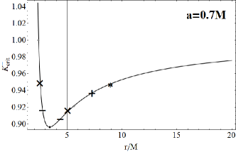
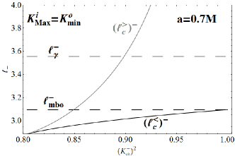
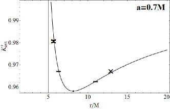
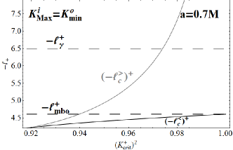
Figure 12: $\ell$corotating couples $\mathrm{C}^{-}_{i}<\mathrm{C}^{-}_{o}$ (upper panels) and $\mathrm{C}^{+}_{i}<\mathrm{C}^{+}_{o}$ (lower panels). Case $K_{\max}^{i}=K_{\min}^{o}$. The specific angular momenta $\ell_{c}^{\lessgtr}:\;V_{eff}(\ell_{i},r_{\max}^{i})\equiv K_{\max}^{i}=K_{\min}^{o}\equiv V_{eff}(\ell_{o},r_{\min}^{i})$ versus $K_{crit}^{2}\in\{K_{\max}^{2},K_{\min}^{2}\}$, where $\ell_{c}^{<}=\ell_{i}$ and $\ell_{c}^{>}=\ell_{o}$, in the region $\mathbf{K0}$ and $\ell>\pm\ell_{\mathrm{mso}}^{\mp}$–see Sec. (3.3). The specific angular momentum $\ell_{\mathrm{mbo}}^{\pm}\equiv\ell_{\pm}(r_{\mathrm{mbo}}^{\pm})$, $\ell_{\gamma}^{\pm}\equiv\ell_{\pm}(r_{\gamma}^{\pm})$ for the marginally bounded orbit, $r_{\mathrm{mbo}}$, and the marginally circular orbit or photon orbit, $r_{\gamma}$, are also plotted.

Finally, condition (43) may also hold for a $\mathrm{C}^{o}_{3}$ ring, because the maximum of the outer configuration is not actually involved. Therefore, the problem will in turn be how small should $\ell_{3}$ to be for the elongation of the inner ring in accretion matching the outer ring. Further discussion regarding the possible loops in the double systems are in Sec. (A.1).

4 Observational evidence of doubled tori disks and their evolution

The systems investigated here and in Pugliese&Stuchlík (2015, 2016a) offer a methodological challenge of describing a set of virtually separated sub-systems as an entire configuration. The double tori of the ringed accretion disk may have different topologies and geometries, being characterized by different rotation laws, giving rise to four different spin-spin alignments with respect to the spin of the central attractor, as sketched in Fig. (4). The evolution of the entire macro-configuration then would result from the evolution of each sub-configuration reaching an interacting phase when the two configurations reach contact eventually. Tori in a double system may collide and merge, or, eventually, turn to generate some feeding–drying processes: the accreting matter from the outer torus of the couple can impact on the inner torus, or the outer torus may be inactive with an active inner torus accreting onto the BH, or both tori may be active. We demonstrate that some configurations will collide for some initial conditions and attractors dimensionless spin. This process likely ends in the formation of a single orbiting toroidal accretion disk. Our studies may provide information also on the SMBH accretion disk formation due to BH interaction with the environment in different stages of its life. The phenomenology associated with these systems may therefore be very wide and we believe that this study could open up a new field of investigation in astrophysics, leading, as proposed also in Sochora et al. (2011); Karas&Sochora (2010); Schee&Stuchlik (2009), to reconstruct the interpretive framework of some phenomena in AGNs environments, thought so far in terms of a single accretion disk, in terms of the multiple accretion disks. The inner edge of the outer ring and the role played by the outer edge of the inner disk should be crucial.

As discussed in Pugliese&Stuchlík (2016a) a strong overflow of matter from a torus of the double configuration, could be also related to a jet formation. Emission may be released in high energy collisions. The enormous energy emitted by the accretion disks in quasars or AGN, in the form of electromagnetic radiation and jets, is generally attributed to the strong gravity of the central black hole when the gravitational binding energy of accreting matter is transformed into radiation.

Finally, we stress that the study of the equilibrium tori could be the starting point for a future analysis of the oscillation modes in the structure of the relativistic ringed disks which can be related to various astrophysical phenomena. The radially oscillating tori of the ringed disk could be related to the high-frequency quasi periodic oscillations observed in non-thermal X-ray emission from compact objects (QPOs), a still obscure feature of the X-ray astronomy related to the inner parts of the disk.

5 Summary and Conclusion

We investigated evolutionary schemes of ringed accretion disks constituted by two toroidal axi-symmetric tori orbiting on the equatorial plane of a central super-massive Kerr black hole. We discussed the emergence of the instability phases for each ring of the macro-configuration in the full general relativistic treatment by considering the effects of the geometry of the Kerr spacetimes on the systems. As results of this analysis we identified particular classes of central Kerr attractors in dependence of their dimensionless spins and the constraints imposed on the evolutionary schemes of the double toroidal system. The schemes outline the topological transition of the tori from an equilibrium topology to the instability depending on the rotation of the tori relative to each other and to the central Kerr black hole. States representing the pair of tori for the four macro-configurations listed in Fig. (7) are summarized in Table (2). We used these blocks to construct the evolutionary schemes in Fig. (8) for a couple of tori in the Schwarzschild spacetime and the $\ell$corotating pairs in a Kerr spacetime, while Figs (9) show the case of $\ell$counterrotating pairs orbiting a Kerr attractor. These couples may be formed only in certain stages of the inner torus evolution for some Kerr attractors. Our analysis in turn sets significant limits on the observational evidence of these systems, providing constraints on the tori–attractor systems imposing limits on the central attractor spins, and relating the attractor to the couple of tori and their evolution from formation to final stage towards accretion or collision. The presented analysis of evolutionary schemes is related to the case of “frozen” Kerr geometry. We here do not follow evolution of ($M$, $a$) parameters of Kerr spacetime. In some cases inclusions of evolution of $a/M$ parameter could introduce some instabilities when some critical values of $a/M$ will be crossed to accretion of corotating or counterrotating matter. The mutation of the geometry determines in general a change of the dynamical properties of the tori, eventually resulting, as argued in Pugliese&Stuchlík (2015), also in an iterative process, which could give rise even to the runaway instability (Abramowicz et al., 1983, 1998; Font&Daigne, 2002a; Rezzolla et al., 2003; Korobkin et al., 2013; Hamersky&Karas, 2013; Pugliese&Quevedo, 2015). This is a theme for future work. Finally, we considered the situation in which the pair of tori may collide either remaining quiescent, or after the emergence of instability from one of the sub-configuration, discussing the mechanisms that, during the tori evolution, could lead to collision. The possible scenarios may, eventually end in the merging of the tori with destruction of the macro-configuration. Note that in the case of $\ell$corotating tori, the outer torus collides, with the inner torus, eventually the tori merge before it can reach the accretion phase, with the consequent destruction of the system (therefore it could not be give rise to a configuration $\mathbf{C}_{\odot}^{x}{}^{2}$ with accretion point $r_{\times}=y_{1}^{i}=y_{3}^{o}$). Similarly, according to the double geodesic structure of the Kerr spacetime there is no outer corotating torus in accretion in a couple with an inner counterrotating torus, as discussed in Sec. (3.2.1) for the couples ${\footnotesize\textbf{()}}^{+}<{\footnotesize\textbf{()}}^{-}$.

Our interest in this investigation was justified by a series of studies and observational evidences supporting the existence of super-massive BHs characterized by multi-accretion episodes during their life-time. These facts justify questioning the relevance of the ringed accretion disks theoretically and changeling them phenomenologically. The presence of such structures modifies substantially we believe, so far assumed scenario of a single disk, taken as the basis of the High Energy Astrophysics, connected with the accretion. New observational effects may then be associated with these complex structures, showing their existence unequivocally. We have different pieces of evidence suggesting what such a situation might be the case. From a theoretical perspective, there are a number of possible physical mechanisms for a ringed disk formation. Our work is related to their dynamics around SMBHs, where the curvature effects become relevant, and the general relativistic treatment adopted here is the most appropriate. There are indeed suggestions for these objects are hosted in the geometries of SMBHs, therefore we assume these systems as most probable environments. It is generally accepted then that the nuclei of most galaxies contain SMBHs, this picture is supported by several studies and agrees with several observational facts. In these environments, SMBHs life may report traces of its host galaxy dynamics. Repeated galaxy mergers may constitute one mechanism for a diversified feeding of a SMBH. Probably, the more immediate situation to think where a ring of matter may be formed is in binary BH systems, and this applies in many astrophysical contexts : X-ray binaries or SMBHs binary systems which are characterized by diversified accretion episodes, feeding BHs with matter and angular momentum. Concerning then possibility of counterrotating disks, which we fully address in the present paper, we refer to well known studies providing strong evidences, and a further fascinating hypothesis of misaligned disks. On this last possibility, there is a quite large literature; we refer for example to Aly et al. (2015); Dogan et al. (2015); Lodato&Pringle (2006). Another mechanism, perfectly fitting particularly with our model of $\ell$corotating tori, foresees a splitting of one accretion disk, resulting in the formation of a tori couple. In other words a ringed accretion disk may result from a fragmentation of a prior single accretion disk, due to a local self-gravitational instability. All these facts lead us to support the suggestion that the existence of such structured objects are likely to be considerably significant in AGNs. Therefore, from the observational point of view, we expect our results have implications in a number of different observational features of AGNs and we have marked some before. On the other hand, it is opening possibilities of different observational evidences for new intriguing phenomena induced by the tori interactions or oscillations. The presence of an inner tori may also enter as a new unexpected ingredient in the accretion-jet puzzle. From a methodological view-point, the study of such systems clearly open an incredible amount of possibilities to be investigated. The analysis introduced here shows the huge number of cases that occurred even within a simple three parameters model (the specific angular momentum $\ell$ the $K$ parameter and the attractor spin-mass ratio). Thus, we have now two possibilities to approach the analysis: by solving numerically in a diversified scenario the equations for a very specific case fixing the disks and attractors parameters. In this way we may also include more ingredients to each disk model, but we lose a general overview of the situation, needing moreover to set some initial configurations. The investigation developed in this work is fixing these two issues: we substantially reduce the parameter space of our model, providing range of variations of the variables and parameters which may fit also to some extent for other disk models, providing also attractor classes on the bases of the tori features. In the end, indicating the attractor which we should chase to find evidences for. We were able to provide also indication of the initial disk couple evolution. Any numerical analysis of more complex situations, sharing the same symmetry of one at last disk, will be compelled with the results presented here.

Particularly, this study, Sec. (3.3), provides strong constraints for the model parameters of the evaluation of the center-of-mass energy in collision between rings which was first evaluated, within the test particle approximation, in Pugliese&Stuchlík (2016c). It was proved that energy efficiency of the collisions increases with increasing dimensionless black hole spin, giving very high values for near-extreme black holes–such systems can be significant for the high energy astrophysics related especially to accretion onto super-massive black holes, and the extremely energetic phenomena in quasars and AGN.

In conclusion we believe our results may be of significance for the high energy astrophysical phenomena, such as the shape of X-ray emission spectra, the X-ray obscuration and absorption by one of the ring, and the extremely energetic radiative phenomena in quasars and AGN that could be observable by the planed X-ray observatory ATHENA ,

Appendix A Graphs

In this section we clarify some aspects of the graphs formalisms used in this work. State lines of the $\ell$corotating couples, used in the monochromatic graph of Fig. (8), are listed in Fig. (14), while the state line for the $\ell$counterrotating couples, used in the bichromatic graphs of Figs (9), are listed in Fig. (13). Samples of loop graphs discussed in this works are in Table (15).

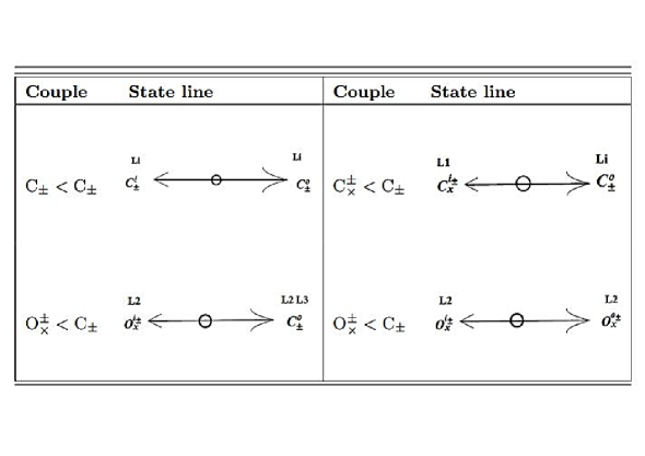
Figure 13: $\ell$corotating couples: state lines of a monochromatic graph (or a bichromatic graphs for a doubled system in a static spacetime) of Fig. (8), corresponding the scheme I and the scheme II of Fig. (4). Main blocks are introduced in Fig. (6).

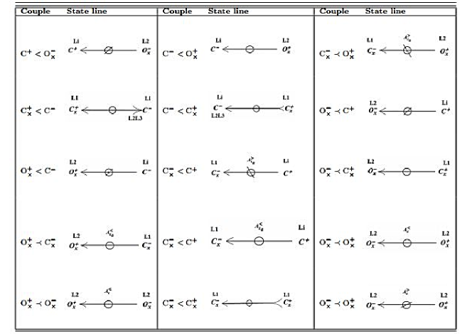
Figure 14: $\ell$counterrotating couple: state lines of bichromatic graph of Figs (9) for a couple of $\ell$counterrotaing disks in a Kerr black hole $a\neq 0$ spacetime, corresponding to the scheme III and the scheme IV in Fig. (4). Main blocks are introduced in Fig. (6).

The evolutive lines generally split the graph into two parts centered around the center: the antecedent section, from which the heads of the arrows converging at the center start, and the subsequent section which is the one onto which the evolutive lines, starting from or crossing the graph center converge with head in the antecedent section–Table (15). A graph may also have only one section. As pointed out in Sec. (3), the evolutive lines may connect state line with different critical sequentiality but not different configuration sequentiality which is preserved during the evolution. In this discussion, vertices which are connected or crossed by an evolutive line, pertain at equal chromaticity. Thus, if the graph center is monochromatic (bichromatic) then the entire graph is monochrome (bichromatic). An evolutive loop is defined as the union of evolutive lines and the vertices they cross, closing on an initial topology as in Table (15), The triple vertix transition $\mathrm{C}\dashrightarrow\mathrm{C}_{\times}\dashrightarrow\mathrm{C}$ is a loop example.

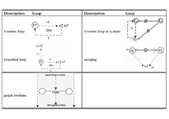
Figure 15: Upper: a loop closed on an equilibrium vertex. The cycle is completed $n$ times with $2n$ evolutive lines (left)- $\pm 1$ is accordingly attached to oriented evolutive lines. Right panel shows an example of such a loop with $n=2$ attached to a state line. Middle: a cycle with an open evolutive line on an topology of accretion represented as a loop with a “branch”(left panel). Right panel shows the merging of two configurations through a closed loop of evolutive lines in which a state line is “contracted” on a vertex. Bottom: graph sections.

A.1 Consideration on the loop emergence

A loop is a closed evolutive line on the graph vertex representing a topological transition of a configuration which would finally restore the initial topology. An example is the drying-feeding process introduced in Pugliese&Stuchlík (2015, 2016a). In this section we briefly discuss possible evolutive scenarios based for the couple of tori on the analysis of the equilibrium and instability states, leaving a more careful and detailed study of the mechanism for such topological transition for future analysis. A loop in general could take place as a consequence of the evolution of one vertex independently by the evolution of the other vertex of the state, or it can be due to a collision among the state vertices. Considering particularly the $\ell$corotating couples we see that separate configurations may be favored for the counterrotating tori having larger distance between the orbital regions and therefore orbiting in the spacetimes of the faster attractors, while the separate states of corotating couples are favored in the geometries of slow attractors–Figs (1). In the case of the counterrotating tori, for larger dimensionless spin of the attractor, the closer and smaller corotating tori should be more frequent since the angular momenta range decreases with the BH spin, reducing therefore the orbital ranges and the distance from the central attractor –Pugliese&Stuchlík (2015, 2016a). The disk extension (elongation on the equatorial plane and the density) depends primarily on the $K$ parameter. On the other hand, the closer to $1$ is the ratio $\ell_{i/o}\gtrapprox 1$, and the smaller are the separated tori, the greater is the possibility of a loop following a geometric correlation and the merging.

To fix the ideas we consider here a simple set up within a simplified schemes based on the following two processes.

1. Loops after independent evolution of the inner ring towards accretion Accretion onto the black hole is associated with loss of matter and angular momentum. In our model both $K$ and the magnitude of the specific angular momentum $\ell$ decrease. Consequently the disk moves towards the attractor possibly shrinking from the maximum elongation $\lambda_{\times}$, reached at the early phases of the process where accretion starts. Following the decrease of the $K$ parameter we assume the accretion could even lead to a stabilization of the inner ring with parameters $\ell_{i}\in\mathbf{L1}$ and $K_{i}\in\mathbf{K0}$. Consequently a $\mathbf{\mathrm{C}^{1}_{\times}\rightarrow\mathrm{C}_{1}}$ transition may rise as a second and last stage of 1-loop–see Table (15). On the other hand, as the magnitude of the specific angular momentum $\ell_{i}$ decreases as well, the ring moves towards the attractor, moving away from the outer ring, while the outer edge of the disk moves inward, finally blocking the loop, preventing any contact with the outer ring, and a transition $\mathbf{\mathrm{C}_{i}\rightarrow\mathrm{C}^{i}_{\times}\rightarrow\mathrm{C}_{i}}$, involving only the inner vertex, can happen.

2. Loops after interaction between the rings In general, an interaction of an inner torus with the surrounding material or collision with the outer torus can lead to increase of matter and $K$, implying destabilization towards a $\mathrm{C}^{1}_{\times}$ or $\mathrm{O}_{\times}^{2}$ phase. Possibly also a split of the disk can occur, increases of the angular momentum which could lead to an $\mathbf{\mathrm{C}_{i}\rightarrow\mathrm{C}^{i}_{\times}}$ transition. However, we note that if the magnitude of the specific momentum increases, the torus moves outward, increasing therefore the probability of collision with the outer ring and, if the momentum magnitude is sufficiently high, i.e. $\ell_{i}\in\{\mathbf{L2},\mathbf{L3}\}$, this prevents emergence of a further stage of accretion. If, on the other hand, $K$ increases in $\mathbf{K0}$, and in $]K_{\min},K_{\max}[$ for $\ell\in\{\mathbf{L1},\mathbf{L2}\}$, the torus outer edge moves outward and its inner margin moves inward, increasing, from one side, the probability of collision with the outer ring, and on the other side, the torus instability finally leading, to the accretion (point 1.), if $\ell_{i}\in\mathbf{L1}$.

The accretion of the inner ring generally blocks the loop: if the inner ring is accreting onto the source, preserving the separation from the outer ring, there is possibility to evolve in a loop, due to the stabilization of the inner vertex that would return under appropriate conditions in the starting equilibrium phase (assuming the ringed disk would not evolve towards a $\mathbf{C}_{\odot}^{x}{}^{2}$ phase, the conditions for this behavior to occur are discussed in Sec. (3.3)). According to the evolutive graph of Fig. (8), the $\mathrm{C}_{\times}^{1}$ disk can return to an equilibrium configuration even for enhanced specific angular momentum, undergoing transition from a $\mathbf{L1}$ range to $\mathbf{L2}$ or $\mathbf{L3}$, through an evolutive line which “ brings ” a new different decoration for the initial vertex. However, such an increase in magnitude of specific angular momentum (due to some specified process) would imply the outer ring to be far enough ($\ell_{o}/\ell_{i}>1$), or to be small enough, to prevent collision.

On the other hand, if the outer disk is not quiescent but it collides with the inner one, then the ringed disk passes from a $\mathbf{C}^{2}$ phase to a $\mathbf{\mathrm{C}}^{2}_{\odot}$ one. This may occur due to decrease (increase) of specific angular momentum $\ell_{o}$ ($\ell_{i}$) or growing of $K_{i}$ or $K_{o}$ (or a combination of these possibilities). Under this very simplified scheme, the interaction between the two tori would lead to a merge in a single disk, destroying therefore the double system. This will happen in competition with a destabilization towards accretion which involves the inner torus only for these couples.

The ringed disk could start, for example, from a $\mathbf{\mathrm{C}}_{\times}^{2}$ phase, where the inner ring is accreting into the source, and it undergoes a $\mathbf{\mathrm{C}}^{\times}_{\odot}{}^{2}$ phase, where the loss of specific angular momentum $\ell_{i}$ and decreasing of $K_{i}$ parameter, should be compared with the support of matter from the outer configuration, which could feed the accretion. As a consequence, this process should be considered as case of collision-inducing-accretion leading possibly to a stabilizing evolutive loop. It may be also induced by an increasing angular momentum, blocking the accretion from the inner torus, causing a merging with the outer torus. Otherwise collision may be predominant, with consequent merging of the two rings in one accreting disk–Table (15).

We can conclude that the double ring systems are less likely to form for corotating rings that would merge or collide that for counterrotating rings: corotating ones are less likely to form around faster attractors, while the formation of counterrotating double rings is favored by the rotation of the attractor. Therefore, we should search for a double system of separated counterrotating rings for fast attractor, while merging should characterize the corotating rings–see Fig. (7). The collision inducing merging can follow the increase of $K$ and the increase of $|\ell_{i}|$, or the increase of $K$ and decrease of $|\ell_{o}|$. The increase of $K_{i}$ is compatible with the onset of the growth phase of $\mathrm{C}^{i}_{\times}$ where in fact $\lambda_{\times}>\lambda$, but if the accretion is associated with a decrease of both $K_{i}$ and $|\ell_{i}|$ (according to 1.)–this favors the separation and prevents the disks collision. To summarize; the processes described in 1. and 2. deal with a competition between the loss of the angular momentum, which causes the tori to shrink and to shift inwardly, and the feeding of matter causing increasing $K$ and possibly $\ell$. Thus, assuming the state $\mathrm{C}^{i}_{\times}<\mathrm{C}_{o}$ does not involve collision, the accretion of the inner ring inevitably leads to separate the tori avoiding the merging, therefore we have to ensure the initial condition for $\lambda_{i}=\lambda^{i}_{\times}$ guaranteing that the two tori are separated, and they remain separated until the outer configuration would change its morphology.

Finally, the role of the radii $r_{\mathcal{M}}$ and $\bar{\mathfrak{r}}_{\mathcal{M}}$ may have impact on the loop production. These radii correspond to the maximum point of the variation of the tori fluid specific angular momenta magnitude $\ell$ with respect to the orbital distance from the attractor, in other words they are solutions of $\partial_{r}\partial_{r}\ell=0$ Pugliese&Stuchlík (2016a). The maximum $\ell_{\mathcal{M}}$ is associated to a torus centered in $r_{\mathcal{M}}$ and with critical point in $\bar{\mathfrak{r}}_{\mathcal{M}}$. This implies that the rings of $\ell$corotating couple with fixed angular momentum magnitude difference $\ell_{o}-\ell_{i}=\epsilon$, are increasingly closer as their angular momentum approaches $\ell_{\mathcal{M}}$ (say, for initial $r_{\min}>r_{\mathcal{M}}$, for $\ell_{i}=\ell_{\mathcal{M}}+\kappa_{i}$ and $\ell_{o}=\ell_{\mathcal{M}}+\kappa_{i}+\epsilon$ with $\epsilon=$constant, and decreasing $\kappa_{i}$) approaching the black hole. The location of momenta $\ell_{\mathcal{M}}^{\pm}\in\mathbf{Li}$ depends on rotation of the torus with respect to the attractor and the dimensionless spin of the attractors– Fig. (1) and Pugliese&Stuchlík (2015, 2016a).

The emergence of the Loops for $\ell$counterrotating couples $\mathrm{C}^{-}<\mathrm{C}^{+}$ We focus on the $\ell$counterrotating couples $\mathrm{C}^{-}<\mathrm{C}^{+}$, analyzed in Sec. (3.2.2). We consider loops involving evolutive phases with accretion, with possible interaction by collision, leading to a $\mathbf{C}^{2}_{\odot}$ ringed disk. First, we note that if evolution towards accretion involves the outer torus only, then collision of the first Roche lobe on the inner torus may be unavoidable. The angular momentum magnitude may decrease, the torus would loose material, finally going inwardly and then making inevitable collision of the first Roche lobe with the inner torus that would acquire momentum and mass. Therefore, this process would give rise to the destruction of the couple, and then there would be no loop. Processes $\mathbf{(a)}$ and $\mathbf{(c)}$ of Eq. (28) and Eq. (29), describe the evolutions of one vertex, however, although similar, their evolutions towards loop is very different. In fact the situation for $\mathbf{(a)}$ is analogue to all the other cases where the inner ring is in accretion as all the $\ell$corotating couples described in Sec. (3.1) and the $\ell$counterrotating ones in the static spacetimes or the $\mathrm{C}_{\times}^{+}<\mathrm{C}^{-}$ addressed in Sec. (3.2.1).d Consequently, a loop may be attached to the unstable vertex of the $\mathrm{C}_{\times}^{-}<\mathrm{C}^{+}$ state as in Fig. (15), when the outer configuration is inert (does not loose angular momentum, otherwise giving rise to a $\mathbf{(b)}$ path or a possible collision with formation of a $\mathbf{C}^{2}_{\odot}$ ringed disk), and no correlation between the two rings torus so that the evolution of the state proceeds through independent evolution of the two vertices. The collision, for loss of angular momentum or thickening of $\mathrm{C}^{+}$, with formation of a $\mathbf{C}_{\odot}^{x}$ system would result in a loop (with correlation) with an outer counterrotating torus which may also be quiescent, i.e., non accreting. In the case of the $\mathbf{(c)}$ process, we can trace the following qualitative consideration regarding the possible generation of loop. A stabilized loop attached to the outer configuration should not be likely in this scenario because the outer accreting torus, losing angular momentum and matter (decreasing $K$ and $-\ell_{+}$), moves inward. The competition of these two processes, however, could be compensated by the fact that material thickens on the inner torus which then should stretch outwardly. In this very simplified model for the evolution of the system after collision, the double system would seem to be destined to merge. However, if the outer torus stabilizes, then in this particular situation the torus may be attached to a loop in which, for example, the outer ring is stable, while the inner one is in accretion, giving rise, for example, to the sequence of processes $\mathbf{(c)}\rightarrow\mathbf{(a)}$ with a loop. Similarly, we can draw some general consideration on the paths $\mathbf{(b)}$ and $\mathbf{(d)}$. A loop in $\mathbf{(b)}$ could be extended for example, by continuing the path $\mathbf{(b)}$ with the $\mathbf{(a)}$ evolution, for stabilization of the inner ring and consequently preceding a $\mathbf{(c)}$ process. It is however necessary to discuss the $\mathrm{C}^{-}_{\times}<\mathrm{C}^{+}_{\times}$ segment, as final state of $\mathbf{(b)}$ and $\mathbf{(d)}$. Assuming that this state will not be constrained by the initial conditions (the different paths) to distinguish the two cases in this way, then the inner torus in accretion onto the black hole and the outer torus in accretion on the inner torus could lead to a possible evolution for stabilizing the outer torus or otherwise a merging.

Appendix B Comments on Table 4

We provide some comments on Table (2). The analysis refers to Fig. (2), where the geodesic complementary structure $\bar{\mathbf{R}}_{\mathrm{N}}$ is represented.

B.0.1 Couples: ${\footnotesize\textbf{()}}^{+}<{\footnotesize\textbf{()}}^{-}$

We consider the decoration of the equilibrium vertices with angular momentum classes for the states ${\footnotesize\textbf{()}}^{+}<{\footnotesize\textbf{()}}^{-}$ of the graph in Fig. (9) and proof of the results of Table (2). The following properties holds:

• All the couples ${\footnotesize\textbf{()}}^{+}_{3}<{\footnotesize\textbf{()}}^{-}$ are ${\footnotesize\textbf{()}}_{3}^{+}<{\footnotesize\textbf{()}}_{3}^{-}$. In fact for ${\footnotesize\textbf{()}}_{3}^{+}<{\footnotesize\textbf{()}}^{-}$, it has to be $\bar{\mathfrak{r}}_{\gamma}^{+}<r_{\min}^{+}<r_{\min}^{-}$, which is realized only for corotating tori ${\footnotesize\textbf{()}}_{3}^{-}$. This means that if the inner ring is counterrotating and sufficiently far from the attractor, then the second (outer) counterrotating ring must be ${\footnotesize\textbf{()}}_{3}^{+}$.
  

• Viceversa, the couples ${\footnotesize\textbf{()}}^{+}<{\footnotesize\textbf{()}}_{3}^{-}$ with $r_{\mathrm{mso}}^{+}<r_{\min}^{+}<r_{\min}^{-}$ and $r_{\min}^{-}>\bar{\mathfrak{r}}_{\gamma}^{+}$ have no constraints on the angular momentum of the inner ring.
  

• The couples ${\footnotesize\textbf{()}}_{2}^{+}<{\footnotesize\textbf{()}}^{-}$ are characterized by the relations $\bar{\mathfrak{r}}_{\mathrm{mbo}}^{+}<r_{\min}^{+}<r_{\min}^{-}$, which implies that for $a>a_{{}_{u}}$, there are only couples ${\footnotesize\textbf{()}}_{2}^{+}<{\footnotesize\textbf{()}}_{3}^{-}$, but if $a<a_{{}_{u}}$, there are ${\footnotesize\textbf{()}}_{2}^{+}<{\footnotesize\textbf{()}}_{3}^{-}$ and ${\footnotesize\textbf{()}}_{2}^{+}<{\footnotesize\textbf{()}}_{2}^{-}$, but not all the configurations ${\footnotesize\textbf{()}}_{2}^{-}$ are eligible.
  

• If ${\footnotesize\textbf{()}}^{+}<{\footnotesize\textbf{()}}_{2}^{-}$, then $r_{\mathrm{mso}}^{+}<r_{\min}^{+}<r_{\min}^{-}<\bar{\mathfrak{r}}_{\gamma}^{-}$, and there are no ${\footnotesize\textbf{()}}_{3}^{+}<{\footnotesize\textbf{()}}_{2}^{-}$ couples, while, remarkably, there are no ${\footnotesize\textbf{()}}^{+}<{\footnotesize\textbf{()}}_{2}^{-}$ couples around attractors with dimensionless spins $a>\breve{a}_{\aleph}$. For slower attractors, $a\in]a_{{}_{u}},\breve{a}_{\aleph}[$, there are only ${\footnotesize\textbf{()}}_{1}^{+}<{\footnotesize\textbf{()}}_{2}^{-}$ couples. Then there is a small class of attractors with the spins $]\tilde{a}_{\aleph},a_{{}_{u}}[$ where $\bar{\mathfrak{r}}_{\mathrm{mbo}}^{-}<r_{\mathrm{mso}}^{+}<\bar{\mathfrak{r}}_{\mathrm{mbo}}^{+}<\bar{\mathfrak{r}}_{\gamma}^{-}$ and, accordingly, there are ${\footnotesize\textbf{()}}_{2}^{+}<{\footnotesize\textbf{()}}_{2}^{-}$ and ${\footnotesize\textbf{()}}_{1}^{+}<{\footnotesize\textbf{()}}_{2}^{-}$. For even lower spins, $a<\tilde{a}_{\aleph}$, where $r_{\mathrm{mso}}^{+}<\bar{\mathfrak{r}}_{\mathrm{mbo}}^{-}<\bar{\mathfrak{r}}_{\mathrm{mbo}}^{+}<\bar{\mathfrak{r}}_{\gamma}^{-}$, there may be both couples ${\footnotesize\textbf{()}}_{1}^{+}<{\footnotesize\textbf{()}}_{2}^{-}$ and ${\footnotesize\textbf{()}}_{2}^{+}<{\footnotesize\textbf{()}}_{2}^{-}$, but not all the ${\footnotesize\textbf{()}}_{2}^{+}$ fulfill this property.
  

• Finally, we focus on the configurations ${\footnotesize\textbf{()}}_{1}$ with $\ell\in\mathbf{L1}$. Analyzing the couples ${\footnotesize\textbf{()}}_{1}^{+}<{\footnotesize\textbf{()}}^{-}$, which satisfy the property $r_{\mathrm{mso}}^{+}<r_{\min}^{+}<r_{\min}^{-}$ then for attractors with $a>\breve{a}_{\aleph}$, there are only couples ${\footnotesize\textbf{()}}_{1}^{+}<{\footnotesize\textbf{()}}_{3}^{-}$, while for $a\in]\tilde{a}_{\aleph},\breve{a}_{\aleph}[$ there are ${\footnotesize\textbf{()}}_{1}^{+}<{\footnotesize\textbf{()}}_{3}^{-}$ and part of ${\footnotesize\textbf{()}}_{1}^{+}<{\footnotesize\textbf{()}}_{2}^{-}$. For slower attractors, $a<\tilde{a}_{\aleph}$, there are also the couples ${\footnotesize\textbf{()}}_{1}^{+}<{\footnotesize\textbf{()}}_{1}^{-}$.
  

• The couples, ${\footnotesize\textbf{()}}^{+}<{\footnotesize\textbf{()}}_{1}^{-}$, for which $r_{\mathrm{mso}}^{+}<r_{\min}^{+}<r_{\min}^{-}<\bar{\mathfrak{r}}_{\mathrm{mbo}}^{-}$, are possible only for $a<\tilde{a}_{\aleph}$ as ${\footnotesize\textbf{()}}_{1}^{+}<{\footnotesize\textbf{()}}_{1}^{-}$.

B.0.2 Couples ${\footnotesize\textbf{()}}^{-}<{\footnotesize\textbf{()}}^{+}$

We deal with the decoration of the equilibrium vertices with angular momentum ranges for the states ${\footnotesize\textbf{()}}^{-}<{\footnotesize\textbf{()}}^{+}$–scheme III of Fig. (4) as in Table (2). We make reference to Fig. (2).

We start with the couple ${\footnotesize\textbf{()}}^{-}={\footnotesize\textbf{()}}_{3}^{-}$, where $\bar{\mathfrak{r}}_{\gamma}^{-}<r_{\min}^{-}<r_{\min}^{+}$. Then for $a>\breve{a}_{\aleph}$, couples ${\footnotesize\textbf{()}}_{3}^{-}<{\footnotesize\textbf{()}}^{+}$ exist for any counterrotating topology. Instead, if the attractor has dimensionless spin $a\in]a_{{}_{u}},\breve{a}_{\aleph}[$ only part of the ${\footnotesize\textbf{()}}_{1}^{+}$ configurations, ${\footnotesize\textbf{()}}_{2}^{+}$ and ${\footnotesize\textbf{()}}_{3}^{+}$ fulfills the condition. For slower attractors, $a<a_{{}_{u}}$, only part of ${\footnotesize\textbf{()}}_{2}^{+}$ and all ${\footnotesize\textbf{()}}_{3}^{+}$ configurations satisfy the condition.

For ${\footnotesize\textbf{()}}^{+}={\footnotesize\textbf{()}}^{+}_{3}$, there is $r_{\mathrm{mso}}^{-}<r_{\min}^{-}<r_{\min}^{+}$, then there could be any corotating topology ${\footnotesize\textbf{()}}_{i}^{-}<{\footnotesize\textbf{()}}^{+}_{3}$.

If ${\footnotesize\textbf{()}}^{-}={\footnotesize\textbf{()}}_{2}^{-}$, there is $\bar{\mathfrak{r}}_{\mathrm{mbo}}^{-}<r_{\min}^{-}<r_{\min}^{+}$ thus, for $a>\tilde{a}_{\aleph}$, any configuration ${\footnotesize\textbf{()}}^{+}$ can be in the couple ${\footnotesize\textbf{()}}_{2}^{-}<{\footnotesize\textbf{()}}^{+}$; for $a<\tilde{a}_{\aleph}$ only part of ${\footnotesize\textbf{()}}_{1}^{+}$ configurations and all ${\footnotesize\textbf{()}}_{2}$ and ${\footnotesize\textbf{()}}_{3}$ are in ${\footnotesize\textbf{()}}_{2}^{-}<{\footnotesize\textbf{()}}^{+}$.

If ${\footnotesize\textbf{()}}^{+}={\footnotesize\textbf{()}}_{2}^{+}$, there is $r_{\mathrm{mso}}^{-}<r_{\min}^{-}<r_{\min}^{+}<\bar{\mathfrak{r}}_{\gamma}^{+}$, any counterrotating configurations may be in the couple.

If ${\footnotesize\textbf{()}}^{-}={\footnotesize\textbf{()}}_{1}^{-}$, there is $r_{\mathrm{mso}}^{-}<r_{\min}^{-}<r_{\min}^{+}$ and ${\footnotesize\textbf{()}}^{+}$ can be in any class of angular momentum with some further restrictions on ${\footnotesize\textbf{()}}_{1}^{+}$ for $a<\tilde{a}_{\aleph}$. If ${\footnotesize\textbf{()}}^{+}={\footnotesize\textbf{()}}_{1}^{+}$, there is $r_{\mathrm{mso}}^{-}<r_{\min}^{-}<r_{\min}^{+}<\bar{\mathfrak{r}}_{\mathrm{mbo}}^{+}$ for $a>a_{{}_{u}}$, ${\footnotesize\textbf{()}}^{-}$ can be in any angular momentum range, and for $a<a_{{}_{u}}$, ${\footnotesize\textbf{()}}^{-}$ can be ${\footnotesize\textbf{()}}_{2}$ or ${\footnotesize\textbf{()}}_{1}$. Note that there is the radius $r_{\mathcal{M}}^{-}$ crossing $\bar{\mathfrak{r}}_{\mathrm{mbo}}^{-}$ for $a\approx 0.35M$.

B.0.3 Comments on the constrained criticality

Here we provide some notes on the results of Table (2) on the criticality order, discussing also the order of decorated state lines for the counterrotating couples of Fig. (14). These constraints on the location of the instability points are consequences of the geodesic structure of spacetime, as represented in Fig. (1). However, we considered also restrictions provided by Pugliese&Stuchlík (2016a), based on the geodesic structure $\bar{\mathbf{R}}_{\mathrm{N}}$ and the relation between the angular momenta $\ell_{\mathrm{N}}$– Fig. (1). For $a>a_{\iota_{a}}$ the geodesic structure implies $\mathrm{C}_{\times}^{-}\prec\mathrm{C}_{\times}^{+}$ where $a_{\iota_{a}}=0.372583M:\;r_{\mathrm{mbo}}^{+}=r_{\mathrm{mso}}^{-}$, where the critical sequentiality is not fixed. However it is possible to prove that the relation $\mathrm{C}_{\times}^{-}\prec\mathrm{C}_{\times}^{+}$ extends also for couples orbiting around slower attractors. In fact, for $a<a_{\iota_{a}}$, there is $r_{\mathrm{mbo}}^{-}<r_{\mathrm{mbo}}^{+}<r_{\mathrm{mso}}^{-}<r_{\mathrm{mso}}^{+}$, However, $r_{\mathrm{mbo}}^{+}\in!\mathrm{C}_{\times}^{-}$, and $r_{\mathrm{mso}}^{+}{\LARGE{\not}}{\in}\mathrm{C}_{\times}^{-}$– this means in particular that $r_{\mathrm{mbo}}^{-}<y_{3}^{-}<r_{\mathrm{mbo}}^{+}<y_{3}^{+}<r_{\mathrm{mso}}^{-}<r_{\mathrm{mso}}^{+}$. therefore there is $\mathrm{C}_{\times}^{-}\prec\mathrm{C}_{\times}^{+}$, which closes the proof. Note that we used the assessment of $r_{\mathrm{mbo}}^{+}\in!\mathrm{C}_{\times}^{-}$ obtained from the considerations in Pugliese&Stuchlík (2016a). Moreover there is $r_{\mathrm{mso}}^{-}{\LARGE{\not}}{\in}\mathrm{C}_{\times}^{+}$ if $\ell_{1}\in]\ell_{\mathrm{mso}}^{+},\ell_{1}(r_{\mathrm{mso}}^{-})[,\;r_{\mathrm{mso}}^{-}{\in}!\mathrm{C}_{\times}^{+},\;\ell_{1}\in]\ell_{1}(r_{\mathrm{mso}}^{-}),\ell_{\mathrm{mbo}}^{+}[$. A similar analysis could be implemented for other topologies. For $a>a_{\iota}$, where $a_{\iota}=0.313708M:\;r_{\gamma}^{+}=r_{\mathrm{mbo}}^{-}$, we have $\mathrm{O}_{\times}^{-}\prec\mathrm{O}_{\times}^{+}$. While there is $\mathrm{O}_{\times}^{-}\prec\mathrm{C}_{\times}^{+}$ in any geometry. Finally, for $a>a_{\gamma_{+}}^{-}=0.638285M:\;r_{\mathrm{mso}}^{-}=r_{\gamma}^{+}$, there is $\mathrm{C}_{\times}^{-}\prec\mathrm{O}_{\times}^{+}$.

References

- Abramowicz (1971) Abramowicz, M. A. 1971, Acta. Astron., 21, 81
- Abramowicz (2008) Abramowicz , M. A. 2008, arXiv:astro-ph/0812.3924
- Abramowicz et al. (1983) Abramowicz, M. A., Calvani, M. & Nobili, L. 1983, Nature, 302, 597–599
- Abramowicz&Fragile (2013) Abramowicz, M. A. & Fragile, P.C. 2013, Living Rev. Relativity, 16, 1
- Abramowicz et al. (2010) Abramowicz, M.A., Jaroszynski, M., Kato, S., et al. 2010, A&A, 521, A15
- Abramowicz et al. (1978) Abramowicz M. A., Jaroszyński M., Sikora M. 1978, A&A, 63, 221
- Abramowicz et al. (1998) Abramowicz, M.A., Karas, V.&Lanza, A. 1998, A&A, 331, 1143
- Abramowicz&Sharp (1983) Abramowicz, M.A., & Sharp, N.A. 1983, Ap&SS, 96, 431
- Abramowicz&Straub (2014) Abramowicz M. A. & Straub O. 2014, Accretion discs, Scholarpedia ,9(8):2408
- Agol&Krolik (2000) Agol, E. & Krolik, J. 2000, ApJ, 528, 161
- Alig et al. (2013) Alig, C., Schartmann, M., Burkert, A., Dolag, K. 2013, ApJ, 771, 2, 119
- Allen et al. (2006) Allen, S. W., Dunn, R.J.H., Fabian, A.C., et al 2006, MNRAS, 1, 372, 21
- Aly et al. (2015) Aly H., Dehnen W., NixonC. & King A. 2015, MNRAS, 449, 1, 65
- Ansorg et al (2003) Ansorg M., Kleinwachter A. & Meinel R. 2003, MNRAS, 339, 515-523
- Bambi et al. (2016) Bambi C., Cardenas-Avendano A., Dauser T., Garcia J. A. & Nampalliwar S. 2016, arXiv:gr-qc/arXiv:1607.00596
- Bonnerot et al. (2016) Bonnerot C., Rossi E. M., Lodato G. & Price D. J. 2016, MNRAS, 455, 2, 2253
- Boyer (1965) Boyer, R.H. 1965, Proc. Camb. Phil. Soc., 61, 527
- Bromley et al. (1998) Bromley, B. C., Miller, W. A. & Pariev, V. I. 1998, Nature, 391, 54, 756
- Carmona-Loaiza et al. (2015) Carmona-Loaiza, J.M., Colpi, M., Dotti, M. & Valdarnini R. 2015, MNRAS, 453, 1608
- Chakrabarti (1990) Chakrabarti, S. K. 1990, MNRAS, 245, 747
- Chakrabarti (1991) Chakrabarti, S. K. 1991, MNRAS, 250, 7
- Chen et al. (2015) Chen, Y., Zhang, X., Zhang, H., et al 2015, Ap&SS, 357, 2, 100
- Coughlin&Begelman (2014) Coughlin, E. R.& Begelman, M. C. 2014, ApJ, 781, 82
- Cremaschini et al. (2013) Cremaschini, C. Kovar J., Slaný P., Stuchlík Z. & Karas V. 2013, ApJS, 209, 15
- De Villiers&Hawley (2002) De Villiers, J-P.& Hawley, J. F. 2002, ApJ, 577, 866
- Dogan et al. (2015) Dogan S., Nixon C., King A. & Price D. J. 2015, MNRAS, 449,2, 1251
- Dyda et al. (2015) Dyda, S., Lovelace, R. V. E., Ustyugova, G.V., Romanova, M. M.&Koldoba, A.V. 2015, MNRAS, 446, 613
- Fender&Munoz-Darias (2015) Fender, R. & Munoz-Darias, T. 2015, arXiv:1505.03526
- Ferreira&Casse (2004) Ferreira, J. & Casse, F. 2004, ApJ, 601, L139
- Font&Daigne (2002a) Font, J. A. & Daigne, F. 2002a, MNRAS, 334, 383
- Font&Daigne (2002b) Font, J. A.& Daigne, F. 2002b, ApJ, 581, L23–L26
- Fragile et al. (2007) Fragile, P. C., Blaes, O. M., Anninois, P. & Salmonson J. D. 2007, ApJ, 668, 417–429
- Fragile et al. (2012) Fragile, P.C., Wilson, J. & Rodriguez, M. 2012, MNRAS, 424, 524
- Gafton et al. (2015) Gafton, E., Tejeda, E., Guillochon, J., Korobkin, O. & Rosswog, S. 2015, MNRAS, 449, 1, 771
- Ghisellini et al. (2014) Ghisellini, G., Tavecchio, F., Maraschi, L., et al. 2014Nature, 515, 376
- Hawley et al. (1984) Hawley J. F., Smarr L. L., Wilson J. R. 1984, ApJ, 277, 296
- Hawley (1987) Hawley J. F. 1987 mnras, 225, 677
- Hawley (1991) Hawley J. F. 1991, ApJ, 381, 496
- Hamersky&Karas (2013) Hamersky, J. & Karas, V. 2013, A&A, 32, 555
- Igumenshchev (2000) Igumenshchev, I. V. & Abramowicz, M. A. 2000, ApJS, 130, 463
- Jaroszynski et al. (1980) Jaroszynski, M., Abramowicz, M. A., Paczynski, B. 1980, Acta Astronm., 30, 1
- Karas&Sochora (2010) Karas, V.&Sochora, V., 2010, ApJ, 725, 2, 1507–1515
- King et al. (2005) King A. R., Lubow S. H., Ogilvie G. I., & Pringle J. E. 2005, MNRAS, 363, 49
- King&Nixon (2013) King A. & Nixon C. 2013, Class. Quantum Gravity, 30, 244006
- King&Pringle (2006) King A. R. & Pringle J. E. 2006, MNRAS, 373, L93
- King et al. (2008) King A. R., Pringle J. E. & Hofmann J. A. 2008, MNRAS, 385, 1621,
- Korobkin et al. (2013) Korobkin, O., Abdikamalov, E., Stergioulas, N., et al. 2013, MNRAS, 431, 1, 354
- Kozlowski et al. (1978) Kozlowski, M., Jaroszynski, M.& Abramowicz, M. A. 1978, A&A 63, 1–2, 209–220.
- Krolik&Hawley (2002) Krolik, J.H. & Hawley, J.F. 2002, ApJ, 573, 754
- Lasota et. al. (2016) Lasota, J.-P., Vieira, R.S.S., Sadowski, A., Narayan, R. & Abramowicz M. A. 2016, A&A., 587, A13
- Lei et al. (2008) Lei, Q., Abramowicz, M. A., Fragile, P. C., Horak, J., Machida, M. & Straub O. 2008, A&A., 498, 471
- Lodato&Pringle (2006) Lodato G. & Pringle J. E. 2006, MNRAS, 368, 1196
- Lovelace&Chou (1996) Lovelace, R. V. E. & Chou, T. 1996, ApJ, 468, L25
- Lovelace et al. (2014) Lovelace, R. V.E., Romanova, M. M., Lii, P.&Dyda, S. 2014, Computational Astrophysics and Cosmology, 1-3
- Lyutikov (2009) Lyutikov, M. 2009, MNRAS, 396, 3, 1545–1552
- Madau (1988) Madau, P. 1988, ApJ, 1, 327, 116-127
- Maitra et al. (2009) Maitra, D., Markoff, S., Brocksopp C., et al. 2009,MNRAS, 398, 4, 1638–1650
- Maraschi&Tavecchio (2003) Maraschi, L.& Tavecchio, F. 2003, ApJ, 593, 667
- Marscher et al. (2002) Marscher, A. P., Jorstad, S. G., Gomez, J. L., et al 2002, Nature, 417, 625–627
- McKinney et al. (2013) McKinney, J.C., Tchekhovskoy, A., & Blandford, R. D. 2013, Science, 339, 49
- Narayan et al. (1998) Narayan R., Mahadevan R.& Quataert E. 1998 arXiv:astro-ph/9803141
- Nealon et al. (2015) Nealon R., Price D. & Nixon C. 2015, MNRAS, 448, 2, 1526
- Ni et al. (2016) Ni Y., Jiang J. & Bambi C. 2016, JCAP, 1609, 09, 014
- Nixon (2012) Nixon C. 2012, MNRAS, 423, 3, 2597-2600
- Nixon et al. (2012a) Nixon C., King A. , Price D. 2012, MNRAS, 422, 3, 2547-2552.
- Nixon et al. (2012b) Nixon C., King A., Price D.& Frank J. 2012, ApJ, 757, 2
- Nixon et al. (2013) Nixon C., King A. & Price D. 2013, MNRAS, 434, 1946
- Novikov&Thorne (1973) Novikov I. D. & Thorne K. S. 1973, Black holes (Les astres occlus), 343 - 450
- Okuda et al. (2005) Okuda T., Teresi, V., Toscano E. & Molteni, D. 2005, MNRAS, 357, 295
- Paczyński (1980) Paczyński, B. 1980, Acta Astron., 30, 4
- Paczyński (2000) Paczyński, B. 2000, astro-ph/0004129.
- Page&Thorne74 (1974) Page Don N. & Thorne Kip S. 1974, ApJ, 191, 499-506
- Pulgiese&Kroon (2012) Pugliese, D.&Kroon, J. A. V. 2012, Gen. Rel. Grav., 44, 2785
- Pugliese&Montani (2013b) 2013, Pugliese D. & Montani G. 2013, Europhys. Lett., 101, 19001
- Pugliese&Montani (2015) Pugliese, D.&Montani. G. 2015, Phys. Rev. D, 91, 083011
- Pugliese et al. (2012) Pugliese, D., Montani, G.,& Bernardini, M. G. 2012, MNRAS, 428, 952
- Pugliese&Quevedo (2015) Pugliese, D.& Quevedo, H. 2015, Eur. Phys. J. C, 75, 5, 234
- Pugliese et al. (2011a) Pugliese, D., Quevedo, H., & Ruffini R. 2011a, Phys. Rev. D, 83, 024021
- Pugliese et al. (2011b) Pugliese, D., Quevedo, H. & Ruffini, R. 2011b, Phys. Rev. D, 84, 044030
- Pugliese et al. (2013) Pugliese, D., Quevedo, H. & Ruffini, R. 2013, Phys. Rev. D, 88, 2, 024042