Zero-order Reverse Filtering

Abstract

In this paper, we study an unconventional but practically meaningful reversibility problem of commonly used image filters. We broadly define filters as operations to smooth images or to produce layers via global or local algorithms. And we raise the intriguingly problem if they are reservable to the status before filtering. To answer it, we present a novel strategy to understand general filter via contraction mappings on a metric space. A very simple yet effective zero-order algorithm is proposed. It is able to practically reverse most filters with low computational cost. We present quite a few experiments in the paper and supplementary file to thoroughly verify its performance. This method can also be generalized to solve other inverse problems and enables new applications.

1 Introduction

Image filtering is a fundamental building block of modern image processing and computer vision systems. Recent advances in this field have led to new models to separate image structure into different layers [18, 33] or to remove unwanted image structure [10, 11, 13, 27, 29, 30] to satisfy the need of various tasks. The success provides the community deep understanding of the capability of image filter.

In this paper, we broadly define “filter” as the operation, in either global optimization or local aggregation way, to smooth images considering edge preserving [4, 9, 10, 11, 13, 18, 20], texture removal [29, 33], or other properties [3, 6, 22, 30]. Unlike other work, we aim to tackle an unconventional problem of

• removing part of or all filtering effect

• without needing to know the exact filter in prior.

We call our method Reverse Filtering or simply DeFilter.

The most related work to DeFilter is probably deconvolution [23, 26]. But this line of research is by nature different – deconvolution is to remove local linear convolution effect, while our goal is to study the reversibility for even nonlinear/optimization based process. Another major discrepancy is that we do not need to know the exact filter form in our method. Therefore, our solver is not related to that of deconvolution at all.

Unique Property

Addressing this DeFilter problem not only is intellectually interesting, but also enables many practical applications. Since our method treats the filtering process as a black box, we can use it to recover images processed by unknown but accessible operations.

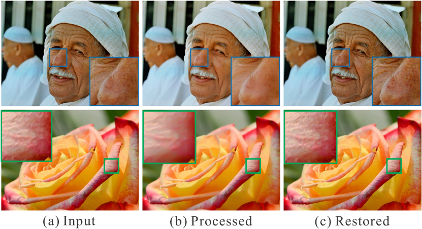
Two examples are shown in Fig. 1. In the first row, the human face is retouched by the Microsoft Selfie App using its “Natural” mode. We have no idea how it is realized. In the second row, noise removal (operation “denoise”) in Photoshop Express is applied. Again, we do not know the algorithm and its implementation details. Interestingly, our method is still able to produce two results that are very close to the original input before processed by the software, as shown in Fig. 1(c). The lost patterns, i.e., freckles and wrinkles on the face and texture of flower, are mostly recovered. To the best of our knowledge, this ability was not explored or exhibited before in filter community.

Figure 1: (a) Original images. (b) Processed images by unknown retouching and denoising algorithms. (c) Our restored images.

Our Approach and Contribution

Our new strategy is to understand the filtering process in metric space where filters are considered as mappings. We provide detailed analysis and propose dividing the image metric space into two sub ones $\Omega$ and $\bar{\Omega}$. In $\Omega$, a filtering operation is strictly a contraction mapping (CM), which leads to a very simple zero-order reverse filtering method to accurately remove unknown effect of filter with low computation cost. Its theoretical correctness and convergence are guaranteed. For filter in $\bar{\Omega}$ that is theoretically not invertible, our algorithm is still effective to reduce its effect in practice, given the fact that most image filters are designed to keep main structure and energy.

Our extensive study shows that the new DeFilter approach works very well on many commonly employed local and global filters, including Gaussian filter, bilateral filter [4], guided image filter [13], adaptive manifold filter [11], rolling guidance filter [33], BM3D denoising [6], and many unknown filters incorporated in commercial software. It also benefits non-blind deconvolution and super-resolution. We will present a large amount of experimental results in the paper and supplementary material.

2 Related Work

Image Filter

Filtering is a basic procedure in computer vision and computational photography. Various filters have been developed for many purposes, such as removing periodical/repetitive textures [24, 29], reducing image noise [3, 6, 30], or scale-aware/edge-aware smoothing [4, 10, 11, 13, 20, 33], to name a few.

Based on the supporting range used, filters can be categorized into local and global ones. For local filters, a pixel value in the output image only depends on its close neighbors. Representative methods include bilateral filter [4], guided filter [13], and anisotropic diffusion [20]. Global methods optimize energy functions defined over all or many pixels. Common strategies include total variation (TV) [22] and weighted least squares [9].

Depending on the property of continuity, most filters are continuous with respect to the input image. Exception includes median-based filters [15, 34] and nearest-neighbor-based methods, such as BM3D [6].

Inverse Problems in Vision

DeFilter belongs to the broad definition of inverse problems in computer vision, where latent causal factors are estimated from observations. Typical inverse problems include image denoising, deblurring, dehazing and super-resolution. For these problems, prior knowledge is often used to regularize the solution space. For example, the dark channel prior [14] is effective for image dehazing. Heavy-tail image gradient prior [21, 25], spectral prior [12] and color prior [17] are used for deblurring. Learning-based approaches exploit information from external data. They include sparse-coding-based methods for super-resolution [32] and denoising [8], as well as DNN-based super-resolution [7], denoising [23], and deconvolution [28].

We note these strategies do not fit our new task of DeFilter. Different image filters have their respective properties, making it difficult to apply general image priors or regularization. Learning-based methods need specific training for each image filter involving parameters, which is also not considered in our solution. Unlike all above methods, we resort to metric space mapping to tackle this new problem.

Figure 2: Illustration of our algorithm regarding operations in each iteration.

3 Reverse Filtering: Method and Conditions

We first investigate the mathematical properties of general filters. Without loss of generality, a filtering process can be described as

$$\mathbf{J}=f(\mathbf{I}),$$ (1)

where $\mathbf{I}$ and $\mathbf{J}$ are the input image and the filtering result. For joint filtering methods [13, 30], we use $\mathbf{I}$ as the guidance image so that $\mathbf{J}$ is still a function of $\mathbf{I}$. Our goal is to estimate $\mathbf{I}$ without the need to compute $f^{-1}(\cdot)$.

Zero-order Reverse Filtering

Our method is simple in terms of programming complexity. The DeFilter results can be achieved using only a few lines of code. The main procedure is an iterative scheme, which updates recovered images according to the filtering effect as

$$\mathbf{X}^{t+1} =\mathbf{X}^{t}+\mathbf{J}^{*}-f(\mathbf{X}^{t}),$$ (2)

where $\mathbf{J}^{*}$ is the filtering result of image $\mathbf{I}^{*}$, with $\mathbf{J}^{*}=f(\mathbf{I}^{*})$. Both $\mathbf{I}^{*}$ and $f(\cdot)$ are unknown in this case. $\mathbf{X}^{t}$ is the current estimate of $\mathbf{I}^{*}$ in the $t$-th iteration. It is a zero-order algorithm because it does not require any derivatives.

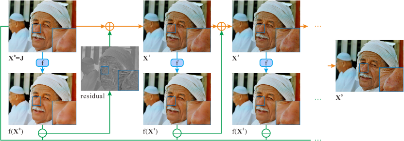
To understand our algorithm, we use the illustration in Fig. 2. We start from $\mathbf{X}^{0}=\mathbf{J}^{*}$, which is the filtered image, as initialization. After re-applying the (unknown) filtering process to $\mathbf{X}^{0}$, details are further suppressed. We then extract the residual $\mathbf{J}^{*}-f(\mathbf{X}^{0})$, which is the difference involving a level of texture and details. The most unconventional step here (highlighted by orange lines in Fig. 2) is that we add the residual back to current estimate $\mathbf{X}^{0}$ to make resulting $\mathbf{X}^{1}$ contain these details. Then we enter another iteration with similar steps. Intriguingly, $\mathbf{X}^{t}$ with increasing $t$ gets closer and closer to $\mathbf{I}^{*}$. For this example, only 5 iterations yield a good DeFilter result.

Despite the simple form, the proposed algorithm does not arbitrarily add back details. Contrarily, in the following we prove for many filters this process is mathematically sound.

3.1 Why Does This Simple Process Work?

The form of Eq. (2) can be considered as a kind of fixed-point iteration. To facilitate analysis, we construct an auxiliary function $g(\mathbf{I})$ as

$$g(\mathbf{I})=\mathbf{I}+(\mathbf{J^{*}}-f(\mathbf{I})).$$ (3)

Eq. (3) is equivalent to Eq. (2) for $\mathbf{X}^{t+1}=g(\mathbf{X}^{t})$. To understand it better, we need contraction mapping defined below to find internal relationship.

Definition 3.1 (Contraction Mapping)

On a metric space $(\mathbb{M},d)$, a mapping $T:\mathbb{M}\rightarrow\mathbb{M}$ is a contraction mapping, if there exists a constant $c\in[0,1)$ such that $d(T(x),T(y))\leq c\cdot d(x,y)$ for all $x,y\in\mathbb{M}$.

With this definition, we take the mapping $T(\cdot)$ as $g(\cdot)$ in Eq. (3). In our case, $\mathbb{M}=\mathbb{R}^{m\times n}$ is the image space of $m\times n$ pixels and $d(x,y)=\|x-y\|$ is the Euclidean distance. It is easy to verify that $(\mathbb{M},d)$ is a complete metric space. With this definition, our algorithm can be explained by following Banach Fixed Point Theorem.

Theorem 3.1 (Banach Fixed Point Theorem)

Let $(\mathbb{M},d)$ be a non-empty complete metric space with a contraction mapping $T:\mathbb{M}\rightarrow\mathbb{M}$. $T$ admits a unique fixed-point $x^{*}$ in $\mathbb{M}$ (i.e., $T(x^{*})=x^{*}$).

Further, $x^{*}$ can be found in the following way. Start with arbitrary state $x_{0}$ in $\mathbb{M}$ and define a sequence $\{x_{n}\}$ as $x_{n}=T(x_{n-1})$. When it converges, $\operatorname*{lim}_{n\rightarrow\infty}x_{n}=x^{*}$.

With this theorem, our algorithm can be understood as actually constructing an image sequence $\{\mathbf{X}^{t}\}$, defined as $\mathbf{X}^{t}=g(\mathbf{X}^{t-1})$. If it satisfies the sufficient condition, it will converge to the unique value $\lim_{t\to\infty}\mathbf{X}^{t}=\mathbf{X}^{*}$. Put differently, the initial $\mathbf{X}^{0}$ is processed by Eq. (2) iteratively and finally reaches $f(\mathbf{X}^{*})\approx\mathbf{J}^{*}$.

Note the sufficient condition that theorem holds is that $g(\mathbf{I})$ forms a contraction mapping, expressed as

$$\|g(\mathbf{I}_{a})-g(\mathbf{I}_{b})\| =\|[\mathbf{I}_{a}-f(\mathbf{I}_{a})]-[\mathbf{I}_{b}-f(\mathbf{I}_{b})]\|$$

$$\leq t\cdot\|\mathbf{I}_{a}-\mathbf{I}_{b}\|,\quad t\in[0,1)$$ (4)

For linear filters, the condition further reduces to

$$\|\mathbf{I}-f(\mathbf{I})\| \leq t\cdot\|\mathbf{I}\|.\quad t\in[0,1)$$ (5)

We analyze the contraction mapping condition in the following regarding different forms of filters. The conclusion is vastly beneficial to the community – several filters satisfy this condition completely. For others, even it does not hold, our zero-order reverse filtering still works to a decent extend to produce satisfying results empirically.

3.2 Convolutional Filter

Figure 3: Reversing convolutional filter. Kernels and their power spectrum are shown in the first column. (a) Image blurred by a Gaussian kernel ($\sigma=2$, kernel size $21\times 21$). (b)-(c) Results after 5 and 20 fixed-point iterations. (d) Image blurred by a disk kernel ($r=3$, kernel size $21\times 21$). (e)-(f) Results after 5 and 15 iterations. Note that high-frequency artifacts start to appear in the 15th iteration.

We start from commonly employed convolutional filter expressed as

$$\mathbf{J}=f(\mathbf{I})=\mathbf{I}\ast\mathbf{K},$$ (6)

where $\ast$ is the convolution operator and $\mathbf{K}$ is the convolution kernel. For ideal Gaussian filter (infinitely large support) and Tikhonov-regularized $L_{2}$-norm image smoothing filter, the spectrum of the kernel contains only real positive numbers, i.e., $\hat{K}_{p}\in(0,1]$. Therefore,

$$\|\mathbf{I}\ast(\mathbf{K}_{\delta}-\mathbf{K})\|=\|\mathbf{\hat{I}}\cdot(\mathbf{1}-\mathbf{\hat{K}})\|\leq t\cdot\|\mathbf{\hat{I}}\|=t\cdot\|\mathbf{I}\|$$ (7)

where $\hat{x}$ denotes Fourier transform, $\cdot$ is point-wised product, $\mathbf{1}$ is an all-one matrix and $p$ indexes pixels. The inequality holds when choosing $t=1-\min_{p}\hat{K}_{p}<1$, which satisfies the condition in Eq. (5). It means these filters can be strictly reversed using fixed-point iteration, if disregarding small numerical errors. As shown in Fig. 3(a)-(c), the DeFilter quality improves consistently in iterations.

For other types of kernels, such as line and disk kernels (Fig. 3(d-f)), $\mathbf{\hat{K}}$ may contain zero, negative or complex values that make $\|1-\hat{K}_{p}\|\geq 1$. In this case, Eq. (5) cannot satisfy arbitrary $\mathbf{I}$. But for $\Omega=\{p\mid\|1-\hat{K}_{p}\|<1\}$, which is the set of frequency components that satisfy Eq. (5), the following inequality still holds.

$$\|\mathbf{\hat{I}}_{\Omega}\cdot(\mathbf{1}_{\Omega}-\mathbf{\hat{K}}_{\Omega})\|\leq t\cdot\|\mathbf{\hat{I}}_{\Omega}\|,$$ (8)

where subscript $\Omega$ denotes that subset from the original image, which only contains frequency points in $\Omega$. $t$ is set to $\max_{p}\|1-\hat{K}_{p}\|$ in this case, such that $t<1$. Due to the linear property of convolution filter, fixed point iteration can be split into two independent sequences as

$$\mathbf{X}^{t+1}=\mathbf{X}^{t+1}_{\Omega}+\mathbf{X}^{t+1}_{\bar{\Omega}}=g(\mathbf{X}^{t}_{\Omega})+g(\mathbf{X}^{t}_{\bar{\Omega}}),$$ (9)

where $\bar{\Omega}$ denotes the complement of $\Omega$. According to previous analysis, $\{\mathbf{X}^{t}_{\Omega}\}$ guarantees to converge to the unique solution $\mathbf{X}^{*}_{\Omega}$, while $\{\mathbf{X}^{t}_{\bar{\Omega}}\}$ could oscillate or diverge.

Fortunately, if we look at the spectrum of kernels, $\Omega$ region covers almost all low-frequency components. For both Gaussian and disk kernels in Fig. 3, $\Omega$ region corresponds to the frequency whose power is greater than 0, which is the majority. Meanwhile, for natural images, the low frequency components dominate their energy. It means that most of useful energy of the original image can be recovered using fixed-point iterations.

In the algorithm level, for the first a few iterations, reverse filtering adds back a lot of details with $\{\mathbf{X}^{t}_{\Omega}\}$, which is the majority, dominating the process. Excessive iterations (over 10) does not change $\{\mathbf{X}^{t}_{\Omega}\}$ much for its near convergence and contrarily amplifies $\{\mathbf{X}^{t}_{\hat{\Omega}}\}$ with high-frequency artifacts (Fig. 3(d-f)). It is worth mentioning that the divergent part contains filter-specific information.

3.3 General Linear Filters

Similar analysis holds for general linear filter of

$$\mathbf{J}=f(\mathbf{I})=\mathbf{A}I,$$ (10)

where $I$ is the vectorized image $\mathbf{I}$, and $\mathbf{A}$ is a square matrix corresponding to linear filter. Singular value decomposition of $(\mathbb{I}-\mathbf{A})$ gives

$$\mathbb{I}-\mathbf{A}=\mathbf{U}\mathbf{S}\mathbf{V}^{*},$$ (11)

where $\mathbb{I}$ is an identity matrix, superscript $*$ means conjugate transpose, $\mathbf{U}$ and $\mathbf{V}$ are unitary matrices, and $\mathbf{S}$ is a diagonal matrix containing singular values. We put these singular values with their squares less than 1 into set $\Omega$ where $\Omega=\{p\mid|diag(\mathbf{S})_{p}|^{2}<1\}$. We further project vectorized image $X$ into two orthogonal subspaces as

$$X_{\Omega}=\mathbf{V}\mathbf{D}_{\Omega}\mathbf{V}^{*}X,\quad X_{\bar{\Omega}}=\mathbf{V}\mathbf{D}_{\bar{\Omega}}\mathbf{V}^{*}X,$$ (12)

where $\mathbf{D}_{\Omega}$ is a diagonal matrix, and $diag(\mathbf{D}_{\Omega})_{p}$ is 1 if $p\in\Omega$, otherwise it is set to 0. $\mathbf{D}_{\bar{\Omega}}=\mathbb{I}-\mathbf{D}_{\Omega}$. We thus have

$$\|(\mathbb{I}-\mathbf{A})X_{\Omega}\| =X^{*}\mathbf{V}\mathbf{D}^{*}_{\Omega}\mathbf{S}^{*}\mathbf{S}\mathbf{D}_{\Omega}\mathbf{V}^{*}X$$

$$=X^{*}\mathbf{V}\mathbf{\Lambda}_{\Omega}\mathbf{V}^{*}X\leq t\cdot\|X\|,$$ (13)

where $\mathbf{\Lambda}_{\Omega}=\mathbf{D}^{*}_{\Omega}\mathbf{S}^{*}\mathbf{S}\mathbf{D}_{\Omega}$ is a diagonal matrix containing only squared singular values in $\Omega$. It is easy to verify that the inequality holds when choosing $t=\max_{p\in\Omega}|diag(\mathbf{S})_{p}|^{2}<1$. Therefore, similar to Eq. (9), iterations can be considered as sum of two independent subsequences in orthogonal subspaces, and subsequent $\{\mathbf{X}^{t}_{\Omega}\}$ can strictly converge to optimal values. In fact, the two separated regions in frequency domain (Fig. 3) are special forms of the orthogonal subspaces we derive in Eq. (12).

The observation that $\Omega$ subspace contains the major energy of a natural image is not by chance. Since most commonly used linear filters are designed to suppress or remove unwanted components like noise and texture while retaining main structures, original structure is mostly included in $\Omega$, whose reversibility is ensured by Eq. (3.3). We will validate it extensively in experiments.

3.4 Other Common Filters

Figure 4: Visualization of reversibility. (a)-(b) Input and filtered images by WLS [9], where the same scan-line pixels are selected as 1D signals. (c)-(d) 1D signals of input (blue), filtered (red) and their difference (yellow). (d) Difference between noise components (yellow) and difference between input images (red).

We extend the idea of considering filter as operations in two separate subspaces. For most image smoothing filters, they are designed to remove the “noise” component. In natural images, noise and texture are small-scale components compared to dominant structure and edges. Taking weighted-least-square [9] as an example, we apply it to two random images shown in Fig. 4. The “noise” components $\mathbf{I}_{a}-f(\mathbf{I}_{a})$ and $\mathbf{I}_{b}-f(\mathbf{I}_{b})$ are the yellow curves in Fig. 4(c-d), respectively. In Fig. 4(e), the absolute difference between the two noise components (in yellow) is much smaller than the absolute difference between the two unfiltered images (in red), which make the filter nearly satisfy the contraction mapping condition in Eq. (3.1) in practice. In the experiment section, we will verify this on lots of filters that are widely used today.

3.5 Zero-order Reverse Filtering Algorithm

Adopting fixed-point iterations for defiltering, our zero-order reverse filter algorithm is summarized in Alg. 1.

INPUT : $\mathbf{J}^{*}$, $f(\cdot)$, $N^{\textrm{iter}}$

OUTPUT : $\mathbf{X}^{*}$

$\mathbf{X}^{0}\leftarrow\mathbf{J}^{*}$ ;

for t:= 1 to $N^{\textrm{iter}}$  do

       $\mathbf{X}^{t}\leftarrow\mathbf{X}^{t-1}+(\mathbf{J}^{*}-f(\mathbf{X}^{t-1}))$

$\mathbf{X}^{*}\leftarrow\mathbf{X}^{N^{\textrm{iter}}}$

Algorithm 1 Zero-order Reverse Filtering

Implementation Remarks

It is noticeable that the implementation of the method is simple without the need to take derivatives. There are two things to pay attention: the implementation of $f$ and determining $N^{\textrm{iter}}$. Some minor complications of $f$ may have a significant impact on the final result. For instance, applying a Gaussian filter with small spatial support range would lead to significantly worse results, as Eq. 7 no longer holds for a truncated Gaussian. As we will shown in Sec. 4.1, there is no single optimal iteration number for all filters, thus it needs to be set empirically.

Figure 5: Results from iterations of reversing adaptive-manifold filter [11].

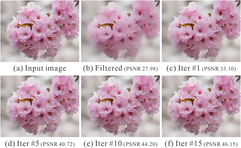
In Fig. 5, we show the intermediate results of this iterative process for reversing adaptive-manifold filter [11]. Applying this filter reduces PSNR to 27.98dB compared to the original image. Applying our DeFilter with 15 iterations raises the PSNR to 46.15dB – there is almost no noticeable difference between the original and defiltered images. Many more examples are provided in the paper and in the supplemental material to manifest its generality.

Our proposed method also has other advantages besides simplicity. It is parameter free. The only parameter is the number of iterations, which can be fixed in prior. It also works well on many nonlinear and complicated filters, such as bilateral filter [4] and guided filter [13]. Even global-optimization-based methods [9] can be reversed effectively.

Differences from Other Residual Strategies

Residual-based enhancement was used for other tasks before – unsharp mask enhances images by adding edge residuals. In super-resolution, the well-known back-projection technique [16] iteratively refines high-res images by back projecting errors. Our method is fundamentally different from these strategies. Unsharp mask is a single-step process and does not recover true details. On the other hand, back-projection is more like a gradient descent method based on the imaging model. Our method does not need to know exact filter model, as illustrated in Fig. 1 and following examples.

Table 1: Evaluation Results on BSD 300 dataset (PSNR)

Filter	GS	BF	BFG	BFPL	GF	AMF	RF	TF	RGF	MF	WMF	BM3D	L0	RTV	WLS	LE
Init GT	27.75	25.50	25.67	27.85	28.21	27.36	27.80	28.75	30.06	26.01	33.00	32.27	26.86	25.34	24.80	29.30
Final GT	41.70	45.28	35.78	32.97	51.05	47.82	28.63	27.61	44.20	N/A	22.98	38.84	28.32	30.27	28.64	7.96
Best GT	41.70	45.28	37.70	36.92	51.05	48.10	31.16	29.21	44.20	26.07	35.43	38.84	28.99	30.27	29.71	44.21
Init DT	36.62	33.12	32.72	33.36	32.49	30.66	29.11	26.85	37.27	37.08	35.72	38.61	31.70	34.84	29.08	37.27
Final DT	79.07	80.50	64.21	54.32	87.94	53.02	60.22	36.00	45.67	N/A	35.65	57.98	36.51	45.38	62.20	45.55
Best DT	79.07	80.50	66.39	54.82	87.94	53.26	60.22	36.28	45.67	38.49	39.16	57.98	38.04	45.38	62.28	45.67

GS: Gaussian Filter, BF: Bilateral Filter [4], BFG: Bilateral Grid [5], BFPL: Permutohedral Lattice [1], GF: Guided Filter [13], AMF: Adaptive Manifold Filter [11], RF: Domain Transform [10], TF: Tree Filter [2], RGF: Rolling Guidance Filter with AMF [33], MF: Median Filter, WMF: Weighted Median Filter [34], BM3D: BM3D Denoise [6], L0: L0 Smooth [27], RTV: Relative Total Variation [29], WLS: Weighted Least Square [9], LE: Local Extrema [24].

4 Experiments

We conduct many experiments to evaluate the effectiveness and the generality of our method on various common filters. Our experiments are conducted on a PC with an Intel Xeon E5 3.7GHz CPU. We use the authors’ implementations for all filters. In order to demonstrate the restoration ability, parameters of these filters are purposely set to large values to produce strong filtering effect. Both qualitative and quantitative results are provided for comparison.

4.1 Quantitative Evaluation

To quantitatively evaluate the restoration accuracy, we build a dataset of 300 images with large appearance and structural variation based on BSD300 from Berkeley segmentation dataset [19]. We apply our method to reverse 16 famous filters, which we believe cover the majority of practical ones. We fix the number of iterations to 50, relatively large for the purpose of analyzing convergence. Our method is initialized as $\mathbf{J}^{*}$.

Two similarity measures based on PSNR are used. Ground truth (GT) error measures the difference between the recovered image and the unfiltered original image. Data-term (DT) error calculates the difference between input filtered image and refiltered version of the recovery result. We calculate initial PSNRs before the first iteration (Init), final PSNRs after 50th iteration (Final). Considering that complicated filters may violate the “reversible condition”, we also report the best PSNRs (Best) achieved in the entire process. The results are listed in Table 1.

Figure 6: Curves of (a) PSRN vs. iteration and (b) Standard deviation (SD) of mean square error (MSE) vs. iteration for common filters.

4.2 Result Analysis

We make several important observations from the results in Table 1. First, DT PSNRs are generally larger than GT ones, which complies with the fact that our method is basically a feedback system based on DT errors. Second, a larger DT PSNR does not necessarily correspond to a larger GT PSNR. For lossy filters, such as median filter (MF) and local extrema filter (LE), the same output can be obtained from different inputs. Thus the defiltered image may not be the same as the original one, which makes perfect sense.

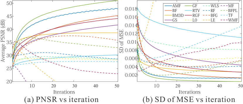
To analyze the convergence of our method on different filters, we plot the PSNR-vs-iteration curves and the curves of standard deviation (SD) of mean square error (MSE) vs. iteration in Fig. 6. For filters that are well reversible, including Gaussian filter (GS), bilateral filter (BF), guided filter (GF), adaptive manifold filter (AMF), rolling guidance filter (RGF), BM3D and relative total variation (RTV), the PSNRs consistently increase.

Figure 7: Image detail recovery. (a) Original noisy input image. (b) Filtered image by BM3D. (c) Defiltered image using our method. Note that the noise patterns between input and our recovered images are very close.

For filters that are partially reversible, such as bilateral grid (BFG), permutohedral lattice (BFPL), domain transform (RF), tree filter (TF), L0 smooth (L0) and weighted least square (WLS), PSNRs increase in early iterations, and then decrease or oscillate in later ones. This complies with our previous theoretical analysis that reversible components dominate images. Thus a good number of, by default 10, iterations can yield satisfying results for most filters.

Finally, for filters that are discontinuous in many places, such as median filter (MF), weighted median filter (WMF), and local extrema filter (LE), our method does not work very well with slightly increased PSNRs in the first a few iterations. For these filters, we claim them as not reversible by our algorithm.

Figure 8: Our method can recover even small-scale image texture by reversing detail-removal filters.

4.3 Recovered Detail Verification

Are the details recovered by our method true signals? In Fig. 7, we apply BM3D denoising on an image, and then use our method to reverse it. Visual inspection indicates that the noise patterns of the defiltered image in Fig. 7(c) is very similar to those of the original image in Fig. 7(a).

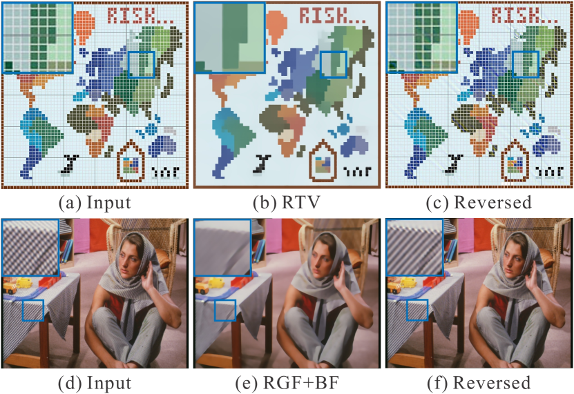
In Fig. 8, we first apply RTV and RGF+BG filters to remove small scale texture and a level of image structures from the input images, then use our method to recover them. Again, our method takes back the small-scale details, consistent with the input. This is because most image filters largely suppress, but do not completely remove these details. The signal residual, albeit not visually prominent, can still help recover the original input. Naturally, if some image structures are completely destroyed in filtering, they cannot be recovered well. This explains the difference of the tablecloth patterns in Fig. 8(f) and (d).

4.4 Robustness

We also evaluate the robustness of our method against lossy JPEG compression applied to the filtered image. In Fig. 9, we first apply AMF to suppress weak edges and texture, followed by standard JPEG compression (MATLAB JPEG encoder with quality 60%, 80%, 90%). The DeFilter results shown in Fig. 9(c)-(e) contain sufficiently recovered image details even under lossy compression.

4.5 More Results and Applications

Zero-order Super-resolution

Single image super-resolution is ill-posed due to information loss. Interestingly, if we define the low-res image generation process as a special down-sampling filter with scale factor $\sigma=2$:

$$f_{SR}(\mathbf{I})=\text{resize}(\text{resize}(\mathbf{I},1/\sigma),\sigma),$$ (14)

we can apply our reverse filtering to rebuild the high-res image. One example is shown in Fig. 10. Bicubic and Lanczos3 interpolation ($\times 2$) achieves PSNRs of 28.99dB and 29.57dB, respectively. Directly applying our method using the Bicubic result as initialization achieves 30.50dB, which is on par with more sophisticated learning-based methods, such as ScSR [31] and SRCNN [7]. Note that our method does not rely on external data or parameter tweaking. Moreover, if we use the results of ScSR [31] and SRCNN [7] as our initialization, we can further improve them as shown in Fig. 10(f)(h). Therefore, our method can be used as a general low-cost post-processing for improving existing super-resolution methods. We would like to point out that the amount of improvement our method can achieve is image-structure-dependent, thus varies with different input images.

Zero-order Nonblind Deconvolution

Figure 9: Reverse filtering under JPEG compression. (a) Original image. (b) Filtered image using AMF. (c)-(e) Our recovered images in 20 iterations under different levels of JPEG compression. Compressed input PSNR (left) and recovered result PSNR (right). (f) Our DeFilter result of (b).

Figure 10: Zero-order super-resolution. (a) Ground truth. (b)-(c) Bicubic and Lanczos3 interpolation. (e)&(g) Results of ScSR [31] and SRCNN [7]. (d)&(f)&(h) Ours results with (b)&(e)&(g) as initialization, respectively.

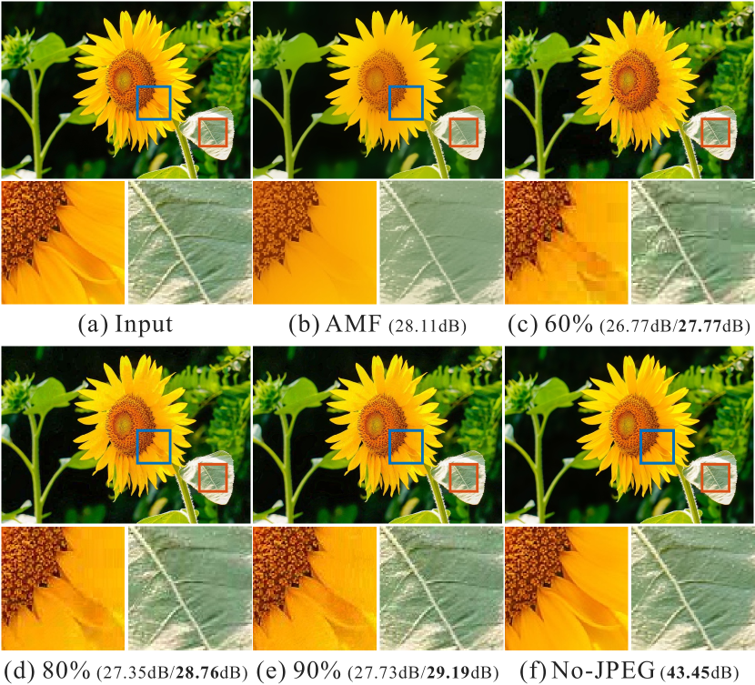
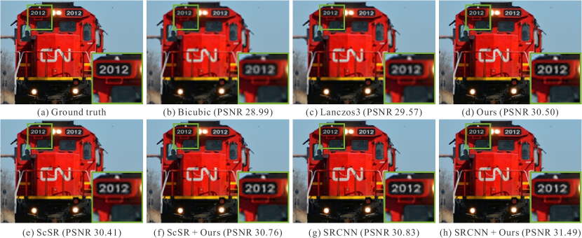
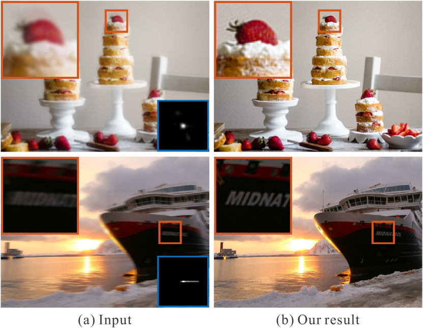
Image convolution is in the common linear form $f_{Conv}(\mathbf{I})=\mathbf{I}\otimes\mathbf{K}$ that our method can handle. In Fig. 11, we apply our method to image deconvolution. Different from other non-blind deconvolution methods, the blur kernel may not be known as long as blur effect can be re-applied. Our method works well for kernels with few zero/negative components in frequency domain to avoid severe information loss and to satisfy Eq. (8).

Applications Against Visual Deceiver

Post-process for hand-held device Apps to beautify human faces and improve image quality is ubiquitous. These filters hide a lot of information that a picture originally capture, which can be sometimes regarded as “visual deceiver”. Our method is the first in its kind to reverse this post-process and show the original look without needing to know the filter that the Apps implemented. Two examples are shown in Fig. 1 and more in our supplementary material due to page limit.

Figure 11: Zero-order nonblind deconvolution. (a) Input image with known blur kernel. (b) Recovered sharp image using our method.

Figure 12: Zero-order restoration for gamma correction and unsharp mask.

Reversal of Other Operators

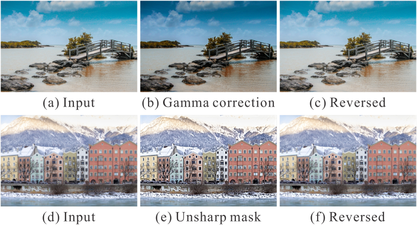
Previous discussions mostly focus on image smoothing processes. Our method can also work well on some different operators. Fig. 12(a)-(c) show an example of gamma correction reverse. Since gamma correctin is basically an element-wise monotonous operation (invertible), it can be easily verified using our iterative method. Fig. 12(d)-(f) show the reversed effect of unsharp mask sharpening method. With mild sharpening parameters, this process also keeps main structures and energies unchanged, which ensures the correctness of our method.

5 Concluding Remarks

We have tackled an unconventional problem of reversing general filter. We have analyzed the condition that a filter can be reversed, and proposed a zero-order reverse filtering method based on fixed-point iterations. Extensive experiments show that this simple method can work well for a wide variety of common filters.

While our method has demonstrated its notable simplicity and generality, it has several limitations. Firstly, depending on filter complexity, the effectiveness may vary. For instance, reversing the median filter is not easy, as reported in Table 1. Secondly, our method cannot bring back details that are completely lost during filtering, as shown in Figs. 8(f) and 9(c).

References

- [1] A. Adams, J. Baek, and M. A. Davis. Fast high-dimensional filtering using the permutohedral lattice. In Computer Graphics Forum, volume 29, pages 753–762. Wiley Online Library, 2010.
- [2] L. Bao, Y. Song, Q. Yang, H. Yuan, and G. Wang. Tree filtering: Efficient structure-preserving smoothing with a minimum spanning tree. IEEE Transactions on Image Processing, 23(2):555–569, 2014.
- [3] A. Buades, B. Coll, and J.-M. Morel. A non-local algorithm for image denoising. In CVPR, volume 2, pages 60–65. IEEE, 2005.
- [4] T. Carlo and M. Roberto. Bilateral filtering for gray and color images. In ICCV, 1998.
- [5] J. Chen, S. Paris, and F. Durand. Real-time edge-aware image processing with the bilateral grid. In ACM Trans. Graph., volume 26, page 103. ACM, 2007.
- [6] K. Dabov, A. Foi, V. Katkovnik, and K. Egiazarian. Image denoising by sparse 3-d transform-domain collaborative filtering. IEEE Transactions on Image Processing, 16(8), 2007.
- [7] C. Dong, C. C. Loy, K. He, and X. Tang. Learning a deep convolutional network for image super-resolution. In ECCV, pages 184–199. Springer, 2014.
- [8] M. Elad and M. Aharon. Image denoising via learned dictionaries and sparse representation. In CVPR, volume 1, pages 895–900. IEEE, 2006.
- [9] Z. Farbman, R. Fattal, D. Lischinski, and R. Szeliski. Edge-preserving decompositions for multi-scale tone and detail manipulation. ACM Trans. Graph., 27(3), 2008.
- [10] E. S. Gastal and M. M. Oliveira. Domain transform for edge-aware image and video processing. ACM Trans. Graph., 30(4):69, 2011.
- [11] E. S. Gastal and M. M. Oliveira. Adaptive manifolds for real-time high-dimensional filtering. ACM Trans. Graph., 31(4):33, 2012.
- [12] A. Goldstein and R. Fattal. Blur-kernel estimation from spectral irregularities. In ECCV, pages 622–635. Springer, 2012.
- [13] K. He, J. Sun, and X. Tang. Guided image filtering. In ECCV, 2010.
- [14] K. He, J. Sun, and X. Tang. Single image haze removal using dark channel prior. IEEE Trans. Pattern Anal. Mach. Intell., 33(12):2341–2353, 2011.
- [15] T. S. Huang, G. J. Yang, and G. Y. Tang. A fast two-dimensional median filtering algorithm. Acoustics, Speech and Signal Processing, IEEE Transactions on, 27(1):13–18, 1979.
- [16] M. Irani and S. Peleg. Improving resolution by image registration. CVGIP: Graphical models and image processing, 53(3):231–239, 1991.
- [17] N. Joshi, C. L. Zitnick, R. Szeliski, and D. J. Kriegman. Image deblurring and denoising using color priors. In CVPR, pages 1550–1557. IEEE, 2009.
- [18] L. Karacan, E. Erdem, and A. Erdem. Structure-preserving image smoothing via region covariances. ACM Trans. Graph., 32(6):176, 2013.
- [19] D. Martin, C. Fowlkes, D. Tal, and J. Malik. A database of human segmented natural images and its application to evaluating segmentation algorithms and measuring ecological statistics. In ICCV, volume 2, pages 416–423, July 2001.
- [20] P. Perona and J. Malik. Scale-space and edge detection using anisotropic diffusion. IEEE Trans. Pattern Anal. Mach. Intell., 12(7):629–639, 1990.
- [21] S. Roth and M. J. Black. Fields of experts: A framework for learning image priors. In CVPR, 2005.
- [22] L. I. Rudin, S. Osher, and E. Fatemi. Nonlinear total variation based noise removal algorithms. Physica D: Nonlinear Phenomena, 60(1):259–268, 1992.
- [23] C. Schuler, H. Burger, S. Harmeling, and B. Scholkopf. A machine learning approach for non-blind image deconvolution. In CVPR, pages 1067–1074, 2013.
- [24] K. Subr, C. Soler, and F. Durand. Edge-preserving multiscale image decomposition based on local extrema. ACM Trans. Graph., 28(5):147, 2009.
- [25] Y. Weiss and W. T. Freeman. What makes a good model of natural images? In CVPR, pages 1–8. IEEE, 2007.
- [26] L. Xu and J. Jia. Two-phase kernel estimation for robust motion deblurring. In ECCV, pages 157–170. Springer, 2010.
- [27] L. Xu, C. Lu, Y. Xu, and J. Jia. Image smoothing via l0 gradient minimization. ACM Trans. Graph., 30(6):174, 2011.
- [28] L. Xu, J. S. Ren, C. Liu, and J. Jia. Deep convolutional neural network for image deconvolution. In NIPS, pages 1790–1798, 2014.
- [29] L. Xu, Q. Yan, Y. Xia, and J. Jia. Structure extraction from texture via relative total variation. ACM Trans. Graph., 31(6):139, 2012.
- [30] Q. Yan, X. Shen, L. Xu, S. Zhuo, X. Zhang, L. Shen, and J. Jia. Cross-field joint image restoration via scale map. In ICCV, 2013.
- [31] J. Yang, J. Wright, T. Huang, and Y. Ma. Image super-resolution as sparse representation of raw image patches. In CVPR, pages 1–8. IEEE, 2008.
- [32] J. Yang, J. Wright, T. S. Huang, and Y. Ma. Image super-resolution via sparse representation. IEEE Transactions on Image Processing, 19(11):2861–2873, 2010.
- [33] Q. Zhang, X. Shen, L. Xu, and J. Jia. Rolling guidance filter. In ECCV, 2014.
- [34] Q. Zhang, L. Xu, and J. Jia. 100+ times faster weighted median filter. In CVPR, 2014.