Global and local spin polarization in heavy ion collisions: a brief overview

Abstract

We give a brief overview about recent developments in theories and experiments on the global and local spin polarization in heavy ion collisions.

1 Introduction

There is inherent correlation between rotation and polarization in materials as shown in the Barnett effect [1] and the Einstein-de Haas effect [2]. We expect that the same phenomena also exist in heavy ion collisions. Huge global angular momenta are generated in non-central heavy ion collisions at high energies [3, 4, 5, 6, 7, 8]. How such huge global angular momenta are transferred to the hot and dense matter created in heavy ion collisions and how to measure them are two core questions in this field. There are some models to address the first question: the microscopic spin-orbital coupling model [3, 4, 8, 9], the statistical-hydro model [10, 11, 12, 13, 14, 15, 16] and the kinetic model with Wigner functions [17, 18, 19, 20]. For the second question, it was proposed that the global angular momentum can lead to the local polarization of hadrons, which can be measured by the polarization of $\Lambda$ hyperons and vector mesons [3, 4].

The global polarization is the net polarization of local ones in an event which is aligned in the direction of the event plane. Recently the STAR collaboration has measured the global polarization of $\Lambda$ hyperons in the beam energy scan program [21, 22]. At all energies below 62.4 GeV, positive polarizations have been found for $\Lambda$ and $\bar{\Lambda}$. On average over all data, the gobal polarization for $\Lambda$ and $\bar{\Lambda}$ are $\Pi_{\Lambda}=(1.08\pm 0.15)\%$ and $\Pi_{\bar{\Lambda}}=(1.38\pm 0.30)\%$. As will be discussed at the end of Sec. 3, this implies that the matter created in ultra-relativistic heavy ion collisions is the most vortical fluid ever produced in the laboratory.

In this note, we give a brief overview about recent developments in theories and experiments on the global and local spin polarization in heavy ion collisions.

2 Theoretical models in particle polarization

In this section we first give a brief introduction to the global orbital angular momentum and local vorticity, which are basic concepts in this topic. Then we introduce three theoretical models which have been widely used in this field. All these models address the same global polarization problem in different angles and are consistent to each other. The spin-orbital coupling model is a microscopic model and the Wigner function and statistical-hydro model are macroscopic models and of statistical type. The thermal average of the local orbital angular momentum in the microscopic model gives the vorticity of the fluid in macroscopic models. The same freeze-out formula for the polarization of fermions are abtained from the Wigner function and statistical-hydro model, which has been used to calulate observables in experiments. The Wigner function model is a quantum kinetic approach where quantum effects like the chiral magnetic and vortical effect and chiral anomaly can be naturally incorporated. The statistical-hydro model is a generalization of the statistical model for a thermal system without rotation to a hydrodynamical one with rotation. With the statistical-hydro model one can easily derive the spin-vorticity coupling term for a system of massive fermions and then the spin polarization density which is proportional to vorticity.

2.1 Global orbital angluar momentum and local vorticity

Let us consider two colliding nuclei with the beam momentum per nucleon $\mathbf{p}_{\mathrm{beam}}\equiv p_{\mathrm{beam}}\mathbf{e}_{z}$ (projectile) and $-\mathbf{p}_{\mathrm{beam}}$ (target). The impact parameter $\mathbf{b}\equiv b\mathbf{e}_{x}$ whose modulus is the transverse distance between the centers of the projectile and target nucleus points from the target to the projectile. The normal direction of the reaction plane or the direction of the global angular momentum is along $\hat{\mathbf{b}}\times\hat{\mathbf{p}}_{\mathrm{beam}}=-\mathbf{e}_{y}$. We should keep in mind that due to event-by-event fluctuations of the nucleon positions, the global orbital angular momentum does not in general point to $-\mathbf{e}_{y}$. The discussion in this subsection is the ideal case only for theoretical simplicity. The magnitude of the total orbital angular momentum $L_{y}$ and the resulting longitudinal fluid shear can be estimated within the wounded nucleon model of particle production [3, 8]. The transverse distributions (integrated over y) of participant nucleons in each nucleus can be written as

$$\frac{dN_{\mathrm{part}}^{\mathrm{P,T}}}{dx}=\int dydz\rho_{A}^{\mathrm{P,T}}(x,y,z,b),$$ (1)

where $\rho_{A}^{\mathrm{P,T}}$ denotes the number of participant nucleons in the projectile and target, respectively. One can use models to estimate $\rho_{A}^{\mathrm{P,T}}$ such as the hard-sphere or Woods-Saxon model. Then we obtain

$$L_{y}=-p_{\mathrm{in}}\int dxx\left(\frac{dN_{\mathrm{part}}^{\mathrm{P}}}{dx}-\frac{dN_{\mathrm{part}}^{\mathrm{P}}}{dx}\right).$$ (2)

The average collective longitudinal momentum per parton can be estimated as

$$p_{z}(x,b;\sqrt{s})=p_{0}\frac{dN_{\mathrm{part}}^{\mathrm{P}}/dx-dN_{\mathrm{part}}^{\mathrm{T}}/dx}{dN_{\mathrm{part}}^{\mathrm{P}}/dx+dN_{\mathrm{part}}^{\mathrm{T}}/dx},$$ (3)

where $p_{0}=\sqrt{s}/[2c(s)]$ denotes the maximum average longtitudinal momentum per parton. The average relative orbital angular momentum for two colliding partons separated by $\Delta x$ in the transverse direction is then $l_{y}\equiv-(\Delta x)^{2}dp_{z}/dx$. Note that $l_{y}$ is expected to be proportional to the local vorticity.

As we all know the strongly coupled quark gluon plasma (sQGP) can be well described by relativistic hydrodynamic models. So the sQGP can be treated as a fluid which is characterized by local quantities such as the momentum, energy and particle-number densities $\mathbf{p}(\mathbf{r})$, $\epsilon(\mathbf{r})$ and $n(\mathbf{r})$, respectively. The total angluar momentum of a fluid can be written as $\mathbf{L}=\int d^{3}r\,\mathbf{r}\times\mathbf{p}(\mathbf{r})$. The fluid velocity is defined by $\mathbf{v}(\mathbf{r})=\mathbf{p}(\mathbf{r})/\epsilon(\mathbf{r})$. In non-relativistic theory, the fluid vorticity is defined by $\boldsymbol{\omega}=\frac{1}{2}\nabla\times\mathbf{v}(\mathbf{r})$. Note that a 1/2 prefactor is introduced in the definition of the vorticity, which is different from normal convention, this is to be consistent to the convention of the vorticity four-vector in relativistic theory. For a rigid-body rotation with a constant angular velocity $\bar{\boldsymbol{\omega}}$, the velocity of a point on the rigid body is given by $v=\bar{\boldsymbol{\omega}}\times\mathbf{r}$. We can verify that $\boldsymbol{\omega}=\frac{1}{2}\nabla\times(\bar{\boldsymbol{\omega}}\times\mathbf{r})=\bar{\boldsymbol{\omega}}$, i.e. for a rigid body in rotation the vorticity is identical to the angular momentum. With the local vorticity, the total angluar momentum can be re-written as $\mathbf{L}=\int d^{3}r\,\epsilon(\mathbf{r})[r^{2}\boldsymbol{\omega}-(\boldsymbol{\omega}\cdot\mathbf{r})\mathbf{r}]$. We see that $\mathbf{L}$ is an integral of the moment of inertia density and the local vorticity. The time evolution of the local velocity and vorticity field can be simulated through the hydrodynamic model [23, 24, 25], the AMPT model [26, 27] or the HIJING model with a smearing technique [28].

2.2 Spin-orbital coupling model

We first consider a simple model for a spin-1/2 quark scattered in a static Yukawa potential $V(\mathbf{r})=e^{-m_{D}|\mathbf{r}|}/(4\pi|\mathbf{r}|)$ with $m_{D}$ being the screening mass. The scattering amplitude is

$$\mathcal{M}(p_{\mathrm{i}},\lambda^{\prime}\rightarrow p_{\mathrm{f}},\lambda)=Qu_{\lambda}^{\dagger}(p_{\mathrm{f}})V(\mathbf{q})u_{\lambda^{\prime}}(p_{\mathrm{i}}),$$ (4)

where $V(\mathbf{q})=1/(\mathbf{q}^{2}+m_{D}^{2})$ is the Fourier transform of $V(\mathbf{r})$ with $\mathbf{q}=\mathbf{p}_{\mathrm{f}}-\mathbf{p}_{\mathrm{i}}$, $Q$ denotes the coupling constant, and $u_{\lambda^{\prime}}(p_{\mathrm{i}})$ and $u_{\lambda}(p_{\mathrm{f}})$ are Dirac spinors of the quark before and after the scattering where $(p_{\mathrm{i}},\lambda^{\prime})$ and $(p_{\mathrm{f}},\lambda)$ are (4-momentum, spin) of the quark in the initial and final state, respectively. The spin-dependent cross section can be obtained

$$\sigma_{\lambda} = \frac{1}{2E_{\mathrm{i}}v_{\mathrm{i}}}\frac{1}{2}\sum_{\lambda^{\prime}}\int\frac{d^{3}p_{\mathrm{f}}}{(2\pi)^{3}2E_{\mathrm{f}}}\bigg{|}\mathcal{M}(p_{\mathrm{i}},\lambda^{\prime}\rightarrow p_{\mathrm{f}},\lambda)\bigg{|}^{2}(2\pi)\delta(E_{\mathrm{f}}-E_{\mathrm{i}}),$$ (5)

where $v_{\mathrm{i}}=|\mathbf{p}_{\mathrm{i}}|/E_{\mathrm{i}}$ and $E_{\mathrm{i}}=\sqrt{\mathbf{p}_{\mathrm{i}}^{2}+m^{2}}$. The polarized and total cross sections can thus be obtained by $\Delta\sigma=\sigma_{+}-\sigma_{-}$ and $\sigma=\sigma_{+}+\sigma_{-}$. In small angle scatterings, the corresponding differential cross sections are in the form $d^{2}\sigma/d^{2}\mathbf{x}_{T}\sim K_{0}(m_{D}|\mathbf{x}_{T}|)$ and $d^{2}\Delta\sigma/d^{2}\mathbf{x}_{T}\sim\mathbf{n}\cdot(\mathbf{x}_{T}\times\mathbf{p}_{\mathrm{i}})$, where $\mathbf{x}_{T}$ is the impact parameter of the scattering in a small local cell [3]. We see that the polarized cross section is proportional to the spin-orbital coupling, $\mathbf{n}\cdot(\mathbf{x}_{T}\times\mathbf{p}_{\mathrm{i}})$, where $\mathbf{n}$ is the spin quantization direction and $\mathbf{L}=\mathbf{x}_{T}\times\mathbf{p}_{\mathrm{i}}$ is the orbital angular momentum. In order to see the connection of the polarization with the spin-ortibal coupling energy $\Delta E_{\mathrm{LS}}$ (as in the nuclear shell model), we rewrite the polarization of the particle for small angle scatterings in the static limit ($\mathbf{p}_{\mathrm{i}}\sim 0$),

$$\Pi\sim\frac{\Delta\sigma}{\sigma}\sim\frac{m_{D}|\mathbf{p}_{\mathrm{i}}|}{E_{\mathrm{i}}(E_{\mathrm{i}}+m)}\sim\frac{m_{D}|\mathbf{p}_{\mathrm{i}}|}{m^{2}}\sim\frac{\Delta E_{\mathrm{LS}}}{E_{0}}$$ (6)

which $\Delta E_{\mathrm{LS}}$ is given by given by

$$\Delta E_{\mathrm{LS}}\sim\mathbf{L}\cdot\mathbf{S}\frac{1}{m^{2}r}\cdot\frac{dV}{dr}\sim\frac{1}{m^{2}}(E_{0}m_{D}^{2})\frac{|\mathbf{p}_{\mathrm{i}}|}{m_{D}}$$ (7)

where $E_{0}$ is an energy scale, $L\sim|\mathbf{p}_{\mathrm{i}}|/m_{D}$ is the angular momentum of the particle, $r^{-1}dV/dr\sim E_{0}m_{D}^{2}$ is the potential gradient divided by the typical range of the potential $r\sim 1/m_{D}$.

One can elaborate the spin-orbital coupling model by considering a more realistic quark-quark scattering at a transverse distance of $\mathbf{x}_{T}$, whose polarized differential cross section is proportional to the spin-orbital coupling $\mathbf{n}\cdot(\mathbf{x}_{T}\times\mathbf{p}_{\mathrm{i}})$, similar to the case of the static potential [8].

2.3 Wigner function method

As the spin-orbital coupling involves a particle’s angular momentum, we have to know a particle’s position and momentum simultaneously. In the classical theory, we use the phase space distribution function of particles, while in quantum theory we have to use the Wigner function, a quantum analogue of the distribution function.

In relativistic quantum theory, the spin four-vector of a massive particle is defined as the Pauli-Lubanski pseudo-vector , $\hat{S}^{\mu}=-\frac{1}{2m}\hat{J}_{\nu\rho}^{\mathrm{S}}\hat{P}_{\sigma}$, which satisfies $[\hat{S}^{\mu},\hat{P}^{\nu}]=0$, $\hat{S}^{\mu}\hat{P}_{\mu}=0$ and $\hat{S}^{\mu}\hat{S}_{\mu}=-S(S+1)$ with $S$ is spin quantum number of the particle. For massive fermions with spin 1/2, we can express its spin tensor density in terms of the Wigner function [19],

$$\left\langle M^{\alpha\beta}(x)\right\rangle = \frac{1}{2}\lim_{y\rightarrow 0}\mathrm{Tr}\left[\gamma_{0}\sigma^{\alpha\beta}\psi(x-\frac{y}{2})\bar{\psi}(x+\frac{y}{2})\right]$$ (8)

$$= \frac{1}{2}\int d^{4}p\mathrm{Tr}\left[\gamma_{0}\sigma^{\alpha\beta}W(x,p)\right].$$

Then we can define the spin tensor component of the Wigner function as

$$\mathscr{M}^{\alpha\beta}(x,p) \equiv \frac{1}{2}\mathrm{Tr}\left[\gamma_{0}\sigma^{\alpha\beta}W(x,p)\right]$$ (9)

$$= \frac{1}{2}\left[-\epsilon^{0\alpha\beta\rho}\mathscr{A}_{\rho}+ig^{\alpha 0}\mathscr{V}^{\beta}-ig^{\beta 0}\mathrm{Tr}(\gamma^{\alpha}W)\right],$$

If we take $\alpha\beta=ij$ (spatial indices), we have a simple relation

$$\mathscr{M}^{ij}(x,p) = \frac{1}{2}\epsilon^{ijk}\mathscr{A}^{k}(x,p),$$ (10)

where $\epsilon_{ijk}$ is 3-dimensional anti-symmetric tensor. We see that one can treat the axial vector component as the spin pseudo-vector phase space density. So the polarization (or spin) pseudo-vector density (with a factor 1/2) is [19]

$$\Pi^{\mu}(x) \approx \frac{1}{2}\int d^{4}p\mathscr{A}^{\mu}(x,p)$$ (11)

at the non-relativistic limit. To match the spin four-vector (Pauli-Lubanski pseudo-vector) in relativistic case, we should multiply a Lorentz factor $E_{p}/m$ as,

$$\Pi^{\mu}(x) \approx \frac{1}{2m}\int d^{4}pE_{p}\mathscr{A}^{\mu}(x,p).$$ (12)

The axial component of the Wigner function can be solved perturbatively in an expansion of powers of space-time derivative $(\partial_{\mu})^{n}$ and field strength $(F_{\mu\nu})^{n}$, whose zeroth and first order solution are

$$A_{(0)}^{\alpha} = m\left[\theta(p_{0})n^{\alpha}(\mathbf{p},\mathbf{n})-\theta(-p_{0})n^{\alpha}(-\mathbf{p},-\mathbf{n})\right]\delta(p^{2}-m^{2})A,$$

$$A_{(1)}^{\alpha}(x,p) = -\frac{1}{2}\hbar\tilde{\Omega}^{\alpha\sigma}p_{\sigma}\frac{dV}{d(\beta p_{0})}\delta(p^{2}-m^{2})-Q\hbar\tilde{F}^{\alpha\lambda}p_{\lambda}V\frac{\delta(p^{2}-m^{2})}{p^{2}-m^{2}},$$ (13)

where $V=f_{+}+f_{-}$ and $A=f_{+}-f_{-}$ with the phase space distribution $f_{s}$ for the spin state $s=\pm$ being defined by

$$f_{s}(x,p) = \frac{2}{(2\pi)^{3}}\left[\theta(p_{0})f_{{\rm FD}}(p_{0}-\mu_{s})+\theta(-p_{0})f_{{\rm FD}}(-p_{0}+\mu_{s})\right],$$ (14)

where $p_{0}\equiv p_{\mu}u^{\mu}$ with $u^{\mu}$ being the fluid velocity, $f_{{\rm FD}}$ is the Fermi-Dirac distribution function, and $\mu_{s}$ is the chemical potential corresponding to the spin state $s$. In Eq. (13), the 4-vector of the spin quantization direction is given by

$$n^{\mu}(\mathbf{p},\mathbf{n}) = \Lambda_{\;\nu}^{\mu}(-\mathbf{v}_{p})n^{\nu}(\mathbf{0},\mathbf{n})=\left(\frac{\mathbf{n}\cdot\mathbf{p}}{m},\mathbf{n}+\frac{(\mathbf{n}\cdot\mathbf{p})\mathbf{p}}{m(m+E_{p})}\right),$$ (15)

where $\Lambda_{\;\nu}^{\mu}(-\mathbf{v}_{p})$ is the Lorentz transformation with $\mathbf{v}_{p}=\mathbf{p}/E_{p}$ and $n^{\nu}(\mathbf{0},\mathbf{n})=(0,\mathbf{n})$ is the spin quantization direction in the rest frame of the fermion.

We note that the polarization pseudo-vector density at the zeroth order is vanishing if $\mu_{s}$ does not depend on the spin $s$. The polarization density at the first order ($\sim\omega^{\alpha},B^{\alpha}$) is obtained by integration over 4-momentum for $A_{(1)}^{\alpha}(x,p)$,

$$\Pi_{(1)}^{\alpha} \approx \frac{1}{2m}\hbar\beta\int\frac{d^{3}p}{(2\pi)^{3}}\left\{\left[E_{p}\omega^{\alpha}+QB^{\alpha}\right]\frac{e^{\beta(E_{p}-\mu)}}{[e^{\beta(E_{p}-\mu)}+1]^{2}}\right.$$ (16)

$$\left.+\left[E_{p}\omega^{\alpha}-QB^{\alpha}\right]\frac{e^{\beta(E_{p}+\mu)}}{[e^{\beta(E_{p}+\mu)}+1]^{2}}\right\},$$

where $Q>0$ is the fermion’s electric charge. The momentum spectra of the polarization pseudo-vector at the freezout hypersurface can be obtained

$$E_{p}\frac{d\Pi^{\alpha}(p)}{d^{3}p} \approx \frac{\hbar}{2m}\beta\frac{1}{(2\pi)^{3}}\int d\Sigma_{\lambda}p^{\lambda}$$ (17)

$$\times\left(\tilde{\Omega}^{\alpha\sigma}p_{\sigma}\pm Q\tilde{F}^{\alpha\sigma}u_{\sigma}\right)f_{\mathrm{FD}}^{\pm}(x,p)\left[1-f_{\mathrm{FD}}^{\pm}(x,p)\right],$$

where $f_{\mathrm{FD}}^{\pm}$ are Dermi-Dirac distribution functions for fermions ($+$) and anti-fermions ($-$), respectively, and $\Sigma_{\lambda}$ denotes the freezeout hypersurface. In Eqs. (16,17), we have used $\tilde{F}^{\rho\lambda}=\frac{1}{2}\epsilon^{\rho\lambda\mu\nu}F_{\mu\nu}$, $\tilde{\Omega}^{\xi\eta}=\frac{1}{2}\epsilon^{\xi\eta\nu\sigma}\Omega_{\nu\sigma}$ with $\Omega_{\nu\sigma}=\frac{1}{2}(\partial_{\nu}u_{\sigma}-\partial_{\sigma}u_{\nu})$, where $\epsilon^{\mu\nu\sigma\beta}$ and $\epsilon_{\mu\nu\sigma\beta}$ are anti-symmetric tensors with $\epsilon^{\mu\nu\sigma\beta}=1(-1)$ and $\epsilon_{\mu\nu\sigma\beta}=-1(1)$ for even (odd) permutations of indices 0123, so we have $\epsilon^{0123}=-\epsilon_{0123}=1$. Instead of $\Omega_{\nu\sigma}$, $\tilde{\Omega}^{\xi\eta}$, $F_{\mu\nu}$ and $\tilde{F}^{\rho\lambda}$, we will also use the vorticity vector $\omega^{\rho}=\frac{1}{2}\epsilon^{\rho\sigma\alpha\beta}u_{\sigma}\partial_{\alpha}u_{\beta}$, the electric field $E^{\mu}=F^{\mu\nu}u_{\nu}$, and the magnetic field $B^{\mu}=\frac{1}{2}\epsilon^{\mu\nu\lambda\rho}u_{\nu}F_{\lambda\rho}$. One can use Eq. (17) to calculate the polarization of spin-1/2 baryons at freezeout hypersurface in heavy ion collisions and compare with experiments.

We note that the above formalism is to describe the polarization of massive fermions with spin 1/2 such as massive quarks or octet baryons of $(1/2)^{+}$. For massless fermions for which the spin vector is not well defined but with helicity or chirality, the polarization can be caused by the chiral magnetic and vortical effect [29, 30, 31].

2.4 Statistical-hydro model

The polarization of a partical in a locally rotating fluid can be described by the statistical-hydro model. The derivation of relativistic hydrodynamics in quantum statistical theory was proposed in late 1970s [11] and early 1980s [10] and further developed by several authors [12, 13, 14, 15, 16]. With the density operator, one can calculate the energy-momentum tensor and current as functions of space-time, $T^{\mu\nu}(x)=\mathrm{Tr}\left[\hat{\rho}\hat{T}^{\mu\nu}(x)\right]\equiv\left\langle\hat{T}^{\mu\nu}(x)\right\rangle$ and $j^{\mu}(x)=\mathrm{Tr}\left[\hat{\rho}\hat{j}^{\mu}(x)\right]\equiv\left\langle\hat{j}^{\mu}(x)\right\rangle$. One can employ the principle of maximum entropy to derive the density operator at local equilibrium. We then use Lagrange multiplier to maximize the entropy under the condition of fixed $T^{\mu\nu}(x)$ and $j^{\mu}(x)$,

$$S = \mathrm{Tr}\left(\hat{\rho}\ln\hat{\rho}\right)+\int_{\Sigma(\tau)}d\Sigma_{\mu}\left\{\left[\left\langle\hat{T}^{\mu\nu}(x)\right\rangle-T^{\mu\nu}(x)\right]\beta_{\nu}(x)\right.$$ (18)

$$\left.-\left[\left\langle\hat{j}^{\mu}(x)\right\rangle-j^{\mu}(x)\right]\zeta(x)\right\},$$

where $\Sigma_{\mu}=\Sigma n_{\mu}$ is the space like hypersurface with $n_{\mu}$ being the time-like vector, $\beta_{\nu}=\beta u_{\nu}$ with $u_{\nu}$ being the fluid velocity. in which leads to $\hat{\rho}_{\mathrm{LE}}$ at local equilibrium (LE),

$$\hat{\rho}_{\mathrm{LE}}=\frac{1}{Z}\exp\left[\int_{\Sigma(\tau)}d\Sigma_{\mu}\left(-T^{\mu\nu}\beta_{\nu}+\zeta\hat{j}^{\mu}\right)\right].$$ (19)

Given $n_{\mu}$, one can determine the local equilibrium value of $\beta^{\alpha}$ and $\zeta$ by $n_{\mu}\left\langle\hat{T}^{\mu\nu}(x)\right\rangle_{\mathrm{LE}}=n_{\mu}T^{\mu\nu}(x)$ and $n_{\mu}\left\langle\hat{j}^{\mu}(x)\right\rangle_{\mathrm{LE}}=n_{\mu}j^{\mu}(x)$.

The global equilibrium of the fluid can be found by imposing the stationary condition under which the density operator does not depend on a particular choice of space-like hypersurface $\Sigma$, so we have $\int_{\Sigma_{1}}d\Sigma_{\mu}\hat{\Phi}^{\mu}=\int_{\Sigma_{2}}d\Sigma_{\mu}\hat{\Phi}^{\mu}$, where $\hat{\Phi}^{\mu}\equiv-\hat{T}^{\mu\nu}\beta_{\nu}+\zeta\hat{j}^{\mu}$, or in another form

$$\oint_{\Sigma_{1}+\Sigma_{2}+\Sigma_{T}}d\Sigma_{\mu}\hat{\Phi}^{\mu}=\int_{V}d^{4}x\partial_{\mu}\hat{\Phi}^{\mu}=0,$$ (20)

where $\Sigma_{T}$ is the transverse surface to $\Sigma_{1}$ and $\Sigma_{2}$. The above equation leads to

$$\partial_{\mu}\hat{\Phi}^{\mu} = -\frac{1}{2}\hat{T}^{\mu\nu}(\partial_{\mu}\beta_{\nu}+\partial_{\nu}\beta_{\mu})+(\partial_{\mu}\zeta)\hat{j}^{\mu}=0.$$

So we obtain the stationary conditions

$$\partial_{\mu}\beta_{\nu}+\partial_{\nu}\beta_{\mu}=0,\;\;\partial_{\mu}\zeta=0,$$ (21)

where the former condition is called the Killing condition whose solution is in the form $\beta^{\mu}=\beta u^{\mu}+\varpi^{\mu\nu}x_{\nu}$, where $\varpi^{\mu\nu}=-\frac{1}{2}(\partial^{\mu}\beta^{\nu}-\partial^{\nu}\beta^{\mu})$. So we obtain the density operator at global equilibrium

$$\hat{\rho}_{\mathrm{GE}}=\frac{1}{Z}\exp\left[-\beta u_{\nu}\hat{P}^{\nu}+\frac{1}{2}\hat{J}^{\nu\rho}\varpi_{\nu\rho}+\zeta\hat{Q}\right],$$ (22)

where $\hat{P}^{\nu}=\int_{\Sigma}d\Sigma_{\mu}\hat{T}^{\mu\nu}$, $\hat{J}^{\nu\rho}=\int_{\Sigma}d\Sigma_{\mu}(x^{\nu}\hat{T}^{\mu\rho}-x^{\rho}\hat{T}^{\mu\nu})$ and $\hat{Q}=\int_{\Sigma}d\Sigma_{\mu}\hat{j}^{\mu}$. We can also add the spin tensor to the angular momentum tensor density $\hat{S}^{\mu;\nu\rho}$:

$$\hat{J}^{\nu\rho} = \int_{\Sigma}d\Sigma_{\mu}(x^{\nu}\hat{T}^{\mu\rho}-x^{\rho}\hat{T}^{\mu\nu}+\hat{S}^{\mu;\nu\rho})$$ (23)

$$= \hat{J}_{\mathrm{OAM}}^{\nu\rho}+\hat{J}_{\mathrm{S}}^{\nu\rho}.$$

The spin tensor $\hat{J}_{\mathrm{S}}^{\nu\rho}$ gives the Pauli-Lubanski pseudo-vector. The expectation value of spin vector is given by $S^{\mu}=\mathrm{Tr}(\hat{\rho}_{\mathrm{GE}}\hat{S}^{\mu})$. Then the polarization is obtained by $\Pi^{\mu}=S^{\mu}/S$.

Since the spin pseudo-vector $\hat{S}^{\mu}$ involves the momentum operator, we need to know a particle’s momentum to evaluate its polarization. In general, this requires the knowledge of the Wigner function, which allows to express the mean values of operators as integrals over space-time and 4-momentum. The mean spin pseudo-vector of a spin-1/2 particle with 4-momentum $p^{\mu}$, produced at $x^{\mu}$ on particlization hypersurface, at the leading order in the thermal vorticity reads [14, 32]

$$\Pi^{\mu}(x,p)=-\frac{1}{8m}[1-f_{\mathrm{FD}}(x,p)]\epsilon^{\mu\nu\sigma\rho}p_{\nu}\varpi_{\sigma\rho},$$ (24)

where $f_{\mathrm{FD}}(x,p)$ is the Fermi-Dirac distribution function. The mean polarization of the particle with 4-momentum $p^{\mu}$ over the particlization hypersurface is given by

$$\Pi^{\mu}(p)=\frac{\int d\Sigma_{\rho}p^{\rho}f_{\mathrm{FD}}(x,p)\Pi^{\mu}(x,p)}{\int d\Sigma_{\rho}p^{\rho}f_{\mathrm{FD}}(x,p)}.$$ (25)

Note that at a constant temperature, Eqs. (24,25) are consistent to Eq. (17) [19]. The parameters in Eq. (25) are those in the hydrodynamical models which give the temperatures, chemical potentials and fluid velocities on the freezeout hypersurface.

3 Experimental measurements of global polarization

The global polarization can be measured by the $\Lambda$ hyperon’s weak decay into a proton and a negatively charged pion. Due to its nature of weak interaction, the proton is emitted preferentially along the direction of the $\Lambda$’s spin in the $\Lambda$’s rest frame, so the parity is broken in the decay process. In this sense, we say that $\Lambda$ is self-analyzing since we can determine the $\Lambda$’s polarization by measuring the daughter proton’s momentum [33]. The solid angle distribution for the daughter proton in the $\Lambda$’s rest frame is given by

$$\frac{dN}{d\Omega^{*}} = \frac{1}{4\pi}\left(1+\alpha_{H}\hat{\mathbf{p}}_{\mathrm{p}}^{*}\cdot\boldsymbol{\Pi}_{\Lambda}\right)=\frac{1}{4\pi}\left(1+\alpha_{H}\Pi_{\Lambda}\cos\theta^{*}\right),$$

where $\hat{\mathbf{p}}_{\mathrm{p}}^{*}$ is the direction of the daughter proton’s momentum in the $\Lambda$’s rest frame, $\boldsymbol{\Pi}_{\Lambda}$ is the $\Lambda$’s polarization vector with its modulus $\Pi_{\Lambda}<1$, $\theta^{*}$ is the angle between the momentum of the daughter proton’s and that of $\Lambda$, and $\alpha_{H}=0.642\pm 0.013$ is the $\Lambda$’s decay constant measured in experiments. The $\Lambda$’s polarization can be determined by an event average of the proton’s momentum direction in the $\Lambda$’s rest frame,

$$\Pi_{\Lambda}=\frac{3}{\alpha_{H}}\left\langle\cos\theta^{*}\right\rangle_{\mathrm{ev}}.$$ (26)

We assume the beam direction is along $\mathbf{e}_{z}$, $\hat{\mathbf{p}}_{\mathrm{beam}}=(0,0,1)$, and the direction of the impact parameter is $\hat{\mathbf{b}}=(\cos\psi_{\mathrm{RP}},\sin\psi_{\mathrm{RP}},0)$ where $\psi_{\mathrm{RP}}$ is the azimuthal angle of the reaction plane. The global polarization $\mathbf{L}$ is along $\hat{\mathbf{b}}\times\hat{\mathbf{p}}_{\mathrm{beam}}=(\sin\psi_{\mathrm{RP}},-\cos\psi_{\mathrm{RP}},0)$. The direction of the daughter proton’s momentum in the $\Lambda$’s rest frame is assumed to be $\hat{\mathbf{p}}_{\mathrm{p}}^{*}=(\sin\theta_{\mathrm{p}}^{*}\cos\phi_{\mathrm{p}}^{*},\sin\theta_{\mathrm{p}}^{*}\sin\phi_{\mathrm{p}}^{*},\cos\theta_{\mathrm{p}}^{*})$. If $\boldsymbol{\Pi}_{\Lambda}$ is in the direction of the global polarization $\mathbf{L}$, we have

$$\cos\theta^{*}=\hat{\mathbf{p}}_{\mathrm{p}}^{*}\cdot\hat{\boldsymbol{\Pi}}_{\Lambda}=\sin\theta_{\mathrm{p}}^{*}\sin(\psi_{\mathrm{RP}}-\phi_{\mathrm{p}}^{*}).$$ (27)

We can obtain the proton’s distribution in $\phi_{\mathrm{p}}^{*}$ after an integration over $\theta_{\mathrm{p}}^{*}$,

$$\frac{dN}{d\phi_{\mathrm{p}}^{*}} = \int_{0}^{\pi}d\theta_{\mathrm{p}}^{*}\sin\theta_{\mathrm{p}}^{*}\frac{dN}{d\Omega^{*}}$$ (28)

$$= \frac{1}{8}+\frac{1}{8}\alpha_{H}\Pi_{\Lambda}\sin(\psi_{\mathrm{RP}}-\phi_{\mathrm{p}}^{*}).$$

Then we obtain $\Pi_{\Lambda}$ by taking an event average of $\sin(\psi_{\mathrm{RP}}-\phi_{\mathrm{p}}^{*})$ [22],

$$\Pi_{\Lambda}=-\frac{8}{\pi\alpha_{H}}\left\langle\sin(\phi_{\mathrm{p}}^{*}-\psi_{\mathrm{RP}})\right\rangle_{\mathrm{ev}}.$$ (29)

The above equation is similar to that used in directed flow measurements [34, 35, 36], which allows us to use the corresponding anisotropic flow measurement technique [37, 38]. The reaction plane angle in Eq. (29) is estimated by calculating the angle of the first order event plane, so we need to correct the final results by the reaction plane resolution $R_{\mathrm{EP}}^{(1)}$. Then we can rewrite Eq. (29) in terms of the first-order event plane angle $\Psi_{\mathrm{EP}}^{(1)}$ and its resolution $R_{\mathrm{EP}}^{(1)}$ [22],

$$\Pi_{\Lambda}=-\frac{8}{\pi\alpha_{H}R_{\mathrm{EP}}^{(1)}}\left\langle\sin\left(\phi_{\mathrm{p}}^{*}-\Psi_{\mathrm{EP}}^{(1)}\right)\right\rangle_{\mathrm{ev}}.$$ (30)

The first-order event plane angle is estimated experimentally by measuring the sidewards deflection of the forward- and backward-going fragments and particles in the STAR’s BBC detectors.

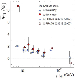
Fig. 1: STAR results for the global $\Lambda$ polarization [21].

The STAR’s recent measurements for the global $\Lambda$ polarization at all collisional energies in the Beam Energy Scan (BES) program are shown in Fig. 1 [21]. At each energy, a positive polarization at the level of $(1.1-3.6)\sigma$ is observed for $\Lambda$ and $\bar{\Lambda}$. Taking all data at different energies into account, the global polarization for $\Lambda$ and $\bar{\Lambda}$ are $\Pi_{\Lambda}=(1.08\pm 0.15)\%$ and $\Pi_{\bar{\Lambda}}=(1.38\pm 0.30)\%$ respectively. Although the experimental uncertainties are too large to state so with confidence, there may be some indication for anti-Lambdas to have larger polarization than Lambdas. Such a difference could in principle be caused by magnetic coupling of their opposite magnetic moments to the magnetic field. However, a quick calculation shows that even for the largest magnetic fields that could be expected in these collisions the effect of this spin-magnetic coupling on the polarization signal would be at most a small fraction of a percent and thus invisible in this experiment. Another source of difference may possibly be due to more Pauli blocking effect for fermions than anti-fermions in lower collisional energies where fermions have non-vanishing chemical potentials [19, 39]. But still such a difference is too small to be observed given the present experimental error bars [21, 32]. The global polarization decreases with increasing collision energy. This is consistent with the observation that longitudinal boost-invariance for the longitudinal expansion becomes a better approximation at higher energies [27, 40], and that a boost-invariant longitudinal flow profile has a vanishing vorticity component orthogonal to the reaction plane.

The fluid vorticity can be estimated from the data by the hydro-statistical model $\omega\approx T(\Pi_{\Lambda}+\Pi_{\bar{\Lambda}})$, where $T$ is the temperature of the fluid at the moment of particle freezeout. The polarization data averaged over collisional energies imply that the vorticity is about $(9\pm 1)\times 10^{21}\,\mathrm{s}^{-1}$. This is much larger than any other fluids that exist in the universe. Then the sQGP created in heavy ion collisions is not only the hottest, least viscous, but also the most vortical fluid that is ever produced in the laboratory.

Acknowledgment. QW thanks M. Lisa and F. Becattini for helpful discussions. QW is supported in part by the Major State Basic Research Development Program (MSBRD) in China under the Grant No. 2015CB856902 and 2014CB845402 and by the National Natural Science Foundation of China (NSFC) under the Grant No. 11535012.

References

- [1] S. Barnett, Rev. Mod. Rev. 7 (2) (1935) 129.
- [2] A. Einstein, W. de Haas, Deutsche Physikalische Gesellschaft, Verhandlungen 17 (1915) 152.
- [3] Z.-T. Liang, X.-N. Wang, Phys. Rev. Lett. 94 (2005) 102301, [Erratum: Phys. Rev. Lett.96,039901(2006)].
- [4] Z.-T. Liang, X.-N. Wang, Phys. Lett. B629 (2005) 20–26.
- [5] S. A. Voloshin, arXiv:nucl-th/0410089.
- [6] B. Betz, M. Gyulassy, G. Torrieri, Phys. Rev. C76 (2007) 044901.
- [7] F. Becattini, F. Piccinini, J. Rizzo, Phys. Rev. C77 (2008) 024906.
- [8] J.-H. Gao, S.-W. Chen, W.-t. Deng, Z.-T. Liang, Q. Wang, X.-N. Wang, Phys. Rev. C77 (2008) 044902.
- [9] S.-w. Chen, J. Deng, J.-h. Gao, Q. Wang, Front. Phys. China 4 (2009) 509–516.
- [10] C. van Weert, Ann. Phys. 140 (1982) 133.
- [11] D. Zubarev, A. Prozorkevich, S. Smolyanskii, Teor. Mat. Fiz. 40 (1979) 394.
- [12] F. Becattini, L. Tinti, Annals Phys. 325 (2010) 1566–1594.
- [13] F. Becattini, Phys. Rev. Lett. 108 (2012) 244502.
- [14] F. Becattini, V. Chandra, L. Del Zanna, E. Grossi, Annals Phys. 338 (2013) 32–49.
- [15] F. Becattini, E. Grossi, Phys. Rev. D92 (2015) 045037.
- [16] T. Hayata, Y. Hidaka, T. Noumi, M. Hongo, Phys. Rev. D92 (6) (2015) 065008.
- [17] J.-H. Gao, Z.-T. Liang, S. Pu, Q. Wang, X.-N. Wang, Phys.Rev.Lett. 109 (2012) 232301.
- [18] J.-W. Chen, S. Pu, Q. Wang, X.-N. Wang, Phys. Rev. Lett. 110 (26) (2013) 262301.
- [19] R.-h. Fang, L.-g. Pang, Q. Wang, X.-n. Wang, Phys. Rev. C94 (2) (2016) 024904.
- [20] R.-h. Fang, J.-y. Pang, Q. Wang, X.-n. Wang, Phys. Rev. D95 (1) (2017) 014032.
- [21] L. Adamczyk, et al., arXiv:1701.06657.
- [22] B. I. Abelev, et al., Phys. Rev. C76 (2007) 024915.
- [23] L. P. Csernai, V. K. Magas, D. J. Wang, Phys. Rev. C87 (3) (2013) 034906.
- [24] L. P. Csernai, D. J. Wang, M. Bleicher, H. Stoecker, Phys. Rev. C90 (2) (2014) 021904.
- [25] L.-G. Pang, H. Petersen, Q. Wang, X.-N. Wang, Phys. Rev. Lett. 117 (19) (2016) 192301.
- [26] Y. Jiang, Z.-W. Lin, J. Liao, Phys. Rev. C94 (4) (2016) 044910.
- [27] H. Li, L.-G. Pang, Q. Wang, X.-L. Xia, arXiv:1704.01507.
- [28] W.-T. Deng, X.-G. Huang, Phys. Rev. C93 (6) (2016) 064907.
- [29] D. E. Kharzeev, L. D. McLerran, H. J. Warringa, Nucl.Phys. A803 (2008) 227–253.
- [30] K. Fukushima, D. E. Kharzeev, H. J. Warringa, Phys. Rev. D78 (2008) 074033.
- [31] D. E. Kharzeev, J. Liao, S. A. Voloshin, G. Wang, Prog. Part. Nucl. Phys. 88 (2016) 1–28.
- [32] F. Becattini, I. Karpenko, M. Lisa, I. Upsal, S. Voloshin, arXiv:1610.02506.
- [33] O. E. Overseth, R. F. Roth, Phys. Rev. Lett. 19 (1967) 391–393.
- [34] J. Barrette, et al., Phys. Rev. C55 (1997) 1420–1430, [Erratum: Phys. Rev.C56,2336(1997)].
- [35] C. Alt, et al., Phys. Rev. C68 (2003) 034903.
- [36] J. Adams, et al., Phys. Rev. C73 (2006) 034903.
- [37] S. Voloshin, Y. Zhang, Z. Phys. C70 (1996) 665–672.
- [38] A. M. Poskanzer, S. A. Voloshin, Phys. Rev. C58 (1998) 1671–1678.
- [39] A. Aristova, D. Frenklakh, A. Gorsky, D. Kharzeev, JHEP 10 (2016) 029.
- [40] I. Karpenko, F. Becattini, arXiv:1610.04717.