Quantum error correction failure distributions: comparison of coherent and stochastic error models
Abstract
We compare failure distributions of quantum error correction circuits for stochastic errors and coherent errors. We utilize a fully coherent simulation of a fault tolerant quantum error correcting circuit for a Steane and surface code. We find that the output distributions are markedly different for the two error models, showing that no simple mapping between the two error models exists. Coherent errors create very broad and heavy-tailed failure distributions. This suggests that they are susceptible to outlier events and that mean statistics, such as pseudo-threshold estimates, may not provide the key figure of merit. This provides further statistical insight into why coherent errors can be so harmful for quantum error correction. These output probability distributions may also provide a useful metric that can be utilized when optimizing quantum error correcting codes and decoding procedures for purely coherent errors.
I Introduction
The theory of fault tolerance and the associated threshold theorem show that given an error rate on physical qubits below some threshold, one can perform a quantum computation with arbitrary accuracy with manageable overhead due to error correction (see e.g., Shor (1995); Steane (1996); Calderbank and Shor (1996); Aharonov and Ben-Or (1997); Knill et al. (1998); Aliferis et al. (2006); Aharonov and Ben-Or (2008); Gottesman (2010); Terhal (2015)). It is well known that the Pauli matrices form a basis for any arbitrary qubit state. Therefore any arbitrary unitary evolution can be written as a linear combination of Pauli matrices. Thus, it is sufficient to correct only for these types of errors in quantum error correction Nielsen and Chuang (2010).
This fact often leads to a logical leap that is not always justified. In particular, in numerical simulations of quantum error correction routines, it is standard practice to only consider stochastic Pauli errors. In some cases such a model is valid. For example, in models of open quantum systems Haake (2001); Breuer and Petruccione (2002); Weiss (2012), the system environment coupling causes the environment to constantly “measure” the qubits. This can cause qubit depolarization, which can be modeled as the mapping of the qubit density matrix
| (1) |
where the terms are classical probabilities. Therefore a completely acceptable interpretation of Eq. (1) is one where with probability no error happens to the wavefunction, and with probability a Pauli , , or error occurs for respectively. This error model is referred to by a variety of different names in the literature. Here we refer to it as the “stochastic Pauli error model”. More generally, an error model can be generated with a larger set of gates than just Pauli gates, but where error gates are randomly inserted in a quantum circuit with classical probabilities. The key characteristic of all these stochastic error models is that the various error configurations all arise from classical probabilities, resulting in no interfering pathways between them.
Coherent errors, which can arise by over- or under-rotations of a quantum gate, were often called “inaccuracies” in the early literature on quantum error correction Knill and Laflamme (1996); Shor (1996). They cannot map to any stochastic error model as they result in a fully coherent evolution with multiple interfering pathways. Proving the existence of threshold in the presence of coherent errors thus requires one to consider the fully coherent sum of interfering fault paths (see, e.g., Sec. 8 in Ref. Aharonov and Ben-Or (2008)). The impact of coherent errors has received renewed attention due to recent results confirming that such errors can be a more severe hurdle for fault-tolerance than stochastic errors Sanders et al. (2016); Kueng et al. (2016).
A more thorough, physics-based justification for when a stochastic error model is an appropriate approximation requires one to consider the entire system-bath interaction. Only when the bath state, entangled with a given error, is orthogonal to all other bath states is the stochastic error model truly appropriate Knill and Laflamme (1996); Knill et al. (1998). Despite these fairly well-known results from the early literature on quantum error correction, the use of stochastic error models is still widely used in numerical simulations to calculate thresholds, including many results that have examined the accuracy of approximating various error channels by stochastic errors Gutiérrez et al. (2013); Geller and Zhou (2013); Puzzuoli et al. (2014); Witzel et al. (2014); Darmawan and Poulin (2016); Gutiérrez et al. (2016). Of course, a significant reason for using this error model this is that these types of errors can be efficiently simulated classically via the Gottesman-Knill theorem Gottesman (1998); Aaronson and Gottesman (2004) if one restricts the set of gates to the Clifford group or a subset (often just Pauli operators are used).
Here, we report that a stochastic error model, has a drastically different logical failure distribution than a failure distribution resulting from coherent errors. To show this, we compare the output failure distributions of a quantum error correction (QEC) memory circuit correcting stochastic Pauli errors to coherent errors. We utilize a numerical simulation of the entire encoded wavefunction, and we examine the failure distribution of the logical state for the Steane [[7,1,3]] code and a distance 3 surface code. We devise failure metrics that avoid the need to implement a final round of perfect error correction and decoding, commonly used when studying the failure characteristics of a logical channel Rahn et al. (2002); Gutiérrez et al. (2013); Darmawan and Poulin (2016); Gutiérrez et al. (2016). Our results show that the output failure distributions are markedly different for the two error models, with coherent errors lead to very broad failure distributions. This suggests that outlier events are much more likely to occur for coherent errors than for stochastic errors, which may provide insight into why they can be so harmful to QEC Sanders et al. (2016); Kueng et al. (2016).
II Numerical Simulation Approach
We numerically simulate two common QEC codes in this paper: the Steane [[7,1,3]] code Steane (1996); Nielsen and Chuang (2010), and the titled-17 surface code Bombin and Martin-Delgado (2007); Horsman et al. (2012); Kitaev (2003). Insertions of errors in the stochastic Pauli (SP) error model are treated as unitary qubit gates, so for both the SP error model and pulse-area error model model the evolution is purely unitary in our simulator. The goal of the report is to determine and compare the output failure probability distributions between these two error models.
Each run starts with a state of Eq. (2):
| (2) |
Here, and , with rand() referring to a uniform pseudo-random number. This covers the Bloch sphere, though not necessarily uniformly.
II.1 Quantum Operations
For a single qubit, the most general evolution is given by an interaction Hamiltonian
| (3) |
where , and are Pauli operators Nielsen and Chuang (2010), the rotation axis is , and couplings with field amplitudes are absorbed into . Evolution is given by , with the propagator:
| (4) | ||||
In these simulations, the shortest path in Hilbert space is used to evolve a gate. Thus, the Hadamard gate is created with an axis and a duration .
The CNOT() gate is implemented using the Hamiltonian:
| (5) |
The projectors ensure that no phase difference accumulates for . This same structure extends to more than one controlling qubit, such as the Toffoli gate. For the controlled-Z gate, replace with .
A measurement of qubit s implemented as
| (6) |
Measurements are instantaneous, and their records are perfect. These are standard assumptions in QEC.
II.2 Error Models
II.2.1 Pauli Error Model
A stochastic Pauli error model is implemented by selecting a set of fault locations and an error rate, . A detailed discussion can be found in Cross et al. (2009). The choice here is conservative: errors are restricted to being only on the codeword qubits, and only before each syndrome measurement. While conservative, this is not unrealistic for this error model as the Pauli errors can be efficiently commuted through a QEC circuit. When the code encounters a fault location, it randomly applies an and error each with probability . Since , all Pauli errors can occur.
II.2.2 Pulse-Area Error Model
For coherent errors, we utilize an error model that we call the pulse-area error model. Coherent manipulations of quantum systems almost universally involve the application of an electromagnetic field, and these are imprecise. Static fields are not independent degrees of freedom, and their fluctuations are tied back to their sources Cohen-Tannoudji et al. (1989); Heitler (1954). Free fields, which include RF pulses in magnetic resonance Ernst et al. (1987) and laser pulses in time domain optical spectroscopy Yariv (1996), are usually well represented by coherent states Mandel and Wolf (1995), and their quantum back-action is quantifiable Barnes and Warren (1999). Commonly, though, these terms can be neglected, and the field amplitudes are -functions in the Hamiltonian that describes a qubit gate. A perfect gate requires the integral of the field amplitude over time (in a rotating frame) to be a fixed angle. The pulse-area error model puts a distribution on this angle. The mean is zero, since systematic errors can be removed with calibration Merrill and Brown (2014).
The pulse-area error model consists of replacing in Eq. (4) with , with uniformly and independently per gate.
| (7) |
All gates in the QEC circuit have and duration . Thus, is related to the fractional jitter in the field amplitudes. For example, for a commercially available pulsed laser sources, Coherent (2016).
III Metric for QEC Failure
This section derives a metric to quantify QEC circuit failure, but adapted to a wavefunction simulation. The prescription here is for the Steane [[7,1,3]] code with a few special considerations required for the surface code noted in Sec. III.2. The focus here is on developing a metric for failure that does not require any perfect measurements, QEC rounds, or decoding, but rather a metric that can be applied to the wavefunction itself.
III.1 Steane Failure Metric
The following definition, from Aliferis et al. (2006), is considered a standard: a QEC circuit that takes any input state with weight errors and outputs a state with weight errors has succeeded; otherwise it has failed. A weight-1 error is defined as having a single Pauli error applied to the state, a weight-2 error has two errors, and so on. The goal is to estimate the probability of failure over many trial runs at fixed . The concatenation threshold is based upon the bound (but there are subtle corrections, see Aliferis et al. (2006)).
This suggests measuring as the portion of that projects into the space of all weight errors. There are several possibilities for this space. Consider using operators, as in a CHP simulation Aaronson and Gottesman (2004). For example, the [[3,1,3]] bit flip correcting code is constructed as in Eq. (8), using and to denote Toffoli and controlled-not gates. The is a projector to that enforces the requirement of fresh ancilla. Any bit-flip error between the encoding and repair steps, by simple matrix multiplication, is seen to never act on qubit 1. This proves the QEC circuit protects the qubit. The point is that does not appear anywhere in this proof. This suggests the QEC failure space for a code is built up from the logical codeword space, as Eq. (9).
| (8) |
| (9) |
These kets form orthonormal states, with , , and for the particular case of Steane’s code. Further, since , one can show . But note that the total Hilbert space of Steane’s code has dimensions. Thus, completely spans it. Since no state could ever leave , it cannot represent a QEC failure criteria, but can.
From the vantage point of Monte Carlo wavefunction simulations, it seems more natural to check if two or more Pauli operators have acted on the starting state for a code. These spaces are built up as
| (10) |
They are orthonormal sets, with and for the particular case of Steane’s code. Since Steane’s code and the surface code are both CSS codes, they correct errors of the form for all and . Checking if has ventured beyond either or is reasonable.
To summarize, we have three metrics to detect a QEC circuit failure, in Eq. (11). For each simulation, when they are 1, the circuit has failed; otherwise, we expect them to be 0.
| (11) |
Technically the sums in Eq. (11) should also extend over the ancilla qubits. However, we assume that measurements are perfect, therefore when we analyze the failure metrics, we know that the ancilla will be in a product state with the data qubits, and thus the sum over them is independent and can be excluded.
Two additional metrics are useful: the projection into , given in Eq. (12), and the fidelity , in Eq. (13). The result implies a perfect repair.
| (12) |
| (13) |
Several useful bounds are shown in Eq. (III.1). Physically, a low implies a low , since is outside of . The inverse does not hold, since a logical error such as on an encoded leaves but . It is also seen that is the most stringent criteria for circuit failure.
| (14) |
Several computational tools to Monte Carlo estimate a pseudo–threshold apparently restrict to be one of the six stabilizer states
| (15) |
This makes drawing distinctions between the metrics in Eq. (11) problematic, as discussed later in this paper.
III.2 Surface Code Failure Metric
The failure metrics for the Steane code was relatively straightforward since all errors map to a unique syndrome. There is a degeneracy in the surface code that complicates this somewhat. We show here how to define a failure metric analogous to that for the Steane code that takes this into account.
The logical state is generated utilizing the parity-check matrix constructed from the stabilizers for the surface code shown later in equation 22. It results in the basis states:
| (16) | ||||
that we can use to construct our logical code space as in equation 9. Note that state is the state under the action of the bitwise-NOT on every binary string within it’s sum. Due to this relation, there is an equivalence in the action of single-qubit errors to both and with respect to the degeneracy of the single-error spaces. For single-qubit errors, there is equivalence of the action of errors, and , and also degeneracies for errors, and . errors are completely non-degenerate. We can therefore construct the failure criteria pertaining to the logical codeword space in the following manner:
| (17) | ||||
where the indices run over all data qubit indices unless otherwise specified. Similarly, for the criteria more natural for the purpose of wavefunction simulations the spaces can be constructed as:
| (18) | ||||
where, again, the indices run over all qubits except for special cases. While it appears that some single-qubit errors have been omitted in the space , the symmetry of the error space ensures that these states have been taken into account. For instance, the state which, through the degeneracy of the errors, can be represented by the state . The assessment of the surface code will incorporate computing the overlap of output wavefunctions with the aforementioned correctable error spaces. Because the surface code is an error correcting code, the sucess criteria and fidelity () given in Eqs. (12) and (13) will be of interest as well.
IV Steane Simulation Results
With failure criteria now defined, we proceed to simulate the error models discussed in Sec. II.2 for Steane’s [[7,1,3]] code. The baseline QEC trial begins by encoding a random qubit. The syndromes, and the errors they detect, are given in Table 1. To ensure fault-tolerance, the three syndromes that check for errors are measured, and then measured again. A loop back occurs if the three sets of syndrome bits do not match. Otherwise, any errors are repaired, and the circuit repeats this for the error detecting syndromes.
The syndrome measurement procedure uses Shor style ancilla It begins by creating a cat state in the 4 ancilla qubits, which is always error free. The test and rejection steps seen in Fig. 6 of Aliferis et al. (2006) are thus not required. After entanglement, the cat state is rotated and read out in the style discussed in Ref. DiVincenzo and Aliferis (2007). Each ancilla is then perfectly re-initialized allowing them to be re-used for the next syndrome.
| Operator | |||||||
|---|---|---|---|---|---|---|---|
| 0 | 1 | 0 | 1 | 1 | 0 | 1 | |
| 0 | 0 | 1 | 1 | 1 | 1 | 0 | |
| 1 | 0 | 0 | 1 | 0 | 1 | 1 | |
| Operator | |||||||
| 0 | 1 | 1 | 0 | 0 | 1 | 1 | |
| 1 | 0 | 1 | 0 | 1 | 0 | 1 | |
| 1 | 1 | 1 | 1 | 0 | 0 | 0 |
IV.1 Pauli Error Model
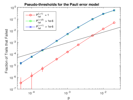
The Steane QEC circuit was run times at nine different values. Histograms of each failure criteria are shown in Fig. 1. The metric is binominally distributed (within numerical accuracy), and has the obvious interpretation. The fraction of trials with for a given is shown by the red curve in Fig. 2. A pseudo-threshold of can be observed. The curve appears similar to examples provided in Svore et al. (2006), and gives confidence that the wavefunction simulations can reproduce the standard pseudo-threshold.

The difficulty with and is that the spaces of Eq. (10) are not aligned with the 6 stabilizer states of Eq. (15). When the code is run with the restricted to be from the set of Eq. (15), then all three metrics in Eq. (11) are binomially distributed. We note here that all Gottesman-Knill and error propagation simulations either require or implicitly assume that input states are Stabilizer states. Even for Pauli errors, this restriction already changes the output failure distribution away from what will actually happen when arbitrarily encoded states must be protected. Since, arbitrary encoded states cannot be abandoned, so how can this result be understood?
First ask: does every non-zero value of or indicate a circuit failure? One way to examine this is to run chains of QEC circuits, where the input of next QEC cycle is the output of the previous one. In such simulations, and transiently drop from 1.0, but then they recover, as seen in Fig. 3 (a). This is a case where weight-1 errors escape a QEC cycle, only to be repaired in the next cycle. By chance, this can occur sequentially, but the metrics remain 0.0, indicating the errors were not fatal ones.
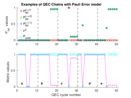
In contrast, if and , then the encoded qubit was corrupted, and clearly the QEC circuit failed. These situations are seen in Fig. 3 (b) to (e). Scatterplots of large samples with did not find any other distinct behaviors, so we consider how to explain each case.
IV.1.1 Case b
Within a single cycle, and , indicating a corrupted but encoded qubit. There are many insertions of 3 Pauli errors that caused this. An example is , , and then , all during the measurement of the error detecting syndromes. Within Steane’s code, , so the repair returns , a properly encoded but corrupted state.
In the failed QEC cycle, it is found that , yet and . The explanation comes by considering the starting state of Eq. (2). For a error, . If the success criteria is set by demanding a threshold, say , then irreparable errors are allowed when encoded states are “lucky” enough to be nearly an eigenstate of that error. For a threshold of , errors are allowed if they shift by on the Bloch sphere. Whether this suffices will depend on the needs of the quantum algorithm.
IV.1.2 Case c
In this trial, two fault locations had errors. Referring to Table 1, the error detection syndromes finished without errors, but a error occurs after the first two syndrome measurements. Since these are checking for errors, the syndrome is (0,0,0). In the second round, a error occurs before the last syndrome. This error should return (1,1,0), but we are on the last syndrome, so (0,0,0) results. As the consistency check is passed, no errors are detected. For this process, an error of escapes. These combination of for are the only errors that distinguish from . In the spirit of Ref. Aliferis et al. (2006), the more stringent weight-1 error criteria of is favored.
IV.1.3 Cases d and e
This appears to show cases where cannot distinguish all errors. Both (d) and (e) would be detected as errors, yet the permanent loss of in (d) is not observed in (e). An examination of several QEC chain trials suggests the answer.
In one case, during the second measurement of the syndromes to detect errors, but just before the consistency check, the following Pauli operators were inserted: S, , S, , S, where implies a syndrome measurement. The first syndrome returns 0. An error should give (1,0,0), so the second syndrome returns 0. At the next error, , and the syndrome for an error is (0,1,0). Thus, the last measurement yields (0,0,0), consistent with the first syndrome measurments. This process allowed a corrupted qubit with a weight-1 error to pass.
In another case, in the second measurement of the error detecting syndromes, this sequence was found: S, , S, , S. As before, this dances around the detection table, and escapes. In the next QEC cycle, however, a single error occurs within the detecting syndromes. Only a error is left for the QEC circuit to repair. By random chance, a process has fixed an unrepairable error.
Three cases involving processes with outcomes like in (e) were examined. They all had the same result: by random chance, the next QEC cycle had a process that converted the weight-2 error into a weight-1 error. As this cannot be assigned to the role of the QEC circuit, we favor the criteria to be a good detector of QEC circuit failure.
IV.2 Pulse-Area Error Model
We now use the pulse area error model outlined in Eq. (7). The reader should keep in mind the following argument in support of a stochastic error model. Consider the QEC circuit as an operator expansion:
| (19) |
There are measurements and unitary gates . Following Eq. (7), and using , this becomes
| (20) |
Now suppose . In that case, the linear terms in simply have each gate . This superficially resembles the Pauli error model: insert a Pauli operator, which cancels the gate, with amplitude at gate . The sum of these terms in Eq. (20) creates . Using the argument in support of the stochastic error model, each syndrome measurement selects one of these terms at a time, so the incoherent sum only needs to be considered. That is very useful, because even if , with the 144 gates of the Steane syndrome extraction circuitry, there are 10,296 dual gate terms to add up, which would be difficult. Yet, in order to fully select one error, 6 syndromes must be measured, even while errors continue to accumulate. The numerical simulation can be used to check this approximation.
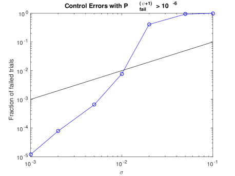
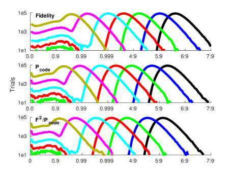
To see how the Steane code handles these pulse area errors, trials with are shown in Fig. 4. All three failure metrics are shown for completeness. First, note that the distributions are very broad. A curve fit to the distribution of showed that roughly 75% of the trials could be described by the log-normal distribution of the form . The maximum likelihood scales as . Employing the critera for failure results in a failure-versus- curve in Fig. 5. For small , it varies as , but comparison with Fig. 2 reveals a much more sigmodial shape.
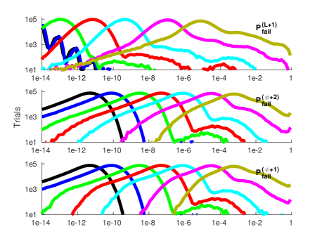
In the Pauli error model, a successful QEC cycle competely restores the encoded qubit. What about the pulse area error model? Fig. 6 shows log-log plots for the distributions of and . Perfect outcomes () are not apparent, but it may be that the part of outside of is still repairable. What about the part inside? Consider the metric in Eq. (21).
| (21) |
It normalizes the part of still in . If it is , then has rotated from within the codeword space. This is an unrepairable error. Histograms of this metric are shown at the bottom of Fig. 6. For , the most likely value of . Thus, a quantum calculation that encodes digital numbers into amplitudes will only be accurate to approximately 4 digits. This distribution scales like , so to achieve float64 precision (16 decimal digits) requires . This is analogous to round-off errors in finite precision classical computers. We note that this error is likely to be reduced as code distance is increased, but lacking a distance 5 simulation we cannot show this.
We finally note that, like the Pauli error model, we have simulated strings of QEC circuits to examine the long term behavior (not shown). This small errors noted here did not grow over multiple cycles, but remained bounded. The QEC circuit is working, but the behavior is much more complicated than the Pauli error model suggests.
V Surface Code Simulation Results
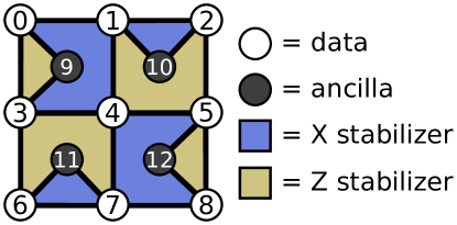
We have demonstrated that the failure distributions for the pulse area error model are qualitatively different than those generated by purely Pauli errors. For completeness we run a similar analysis on a surface code simulation. The particular variant we choose is the tilted-17 surface code, which is a variation on the distance 3 surface code that requires less data and ancilla qubits compared to conventional distance 3 surface code Bombin and Martin-Delgado (2007); Horsman et al. (2012); Kitaev (2003). A diagram of the qubit and stabilizer layout of the code is shown in Fig. 7. A list of the eight stabilzers are shown below:
|
|
(22) |
The measurement of the weight-4 stabilizers are scheduled in such a way that single qubit errors on the ancilla qubits propagate to, at most, two-qubit errors on the data in a manner such that the propagation direction is perpendicular to the direction of the logical operator of the surface code resulting in fault-tolerance Tomita and Svore (2014). An additional requirement for fault-tolerance is the repetitive measurement (typically for measurement rounds) of the stabilizers before applying a correction operation.
For this study, a lookup table decoder was implemented for error correction Tomita and Svore (2014). This method utilizes a small set of syndrome processing rules that is equivalent to applying a minimum weight perfect matching algorithm Fowler et al. (2012); Edmonds (1965a, b) to only nearest neighbor syndrome pairs Tomita and Svore (2014) which, for a distance 3 code, is sufficient for error correction. There is some freedom to how one can schedule the syndrome extraction routine. For this manuscript we use a “single-shot” detection and correction cycle where we perform followed by stabilizer measurements, repeat them three times to ensure fault tolerance, then decoding/correction is performed once.
V.1 Pauli Error Model
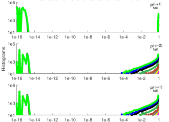
The “single-shot” error correction routines were each run times at each error rate = 0.000001, 0.0000025, 0.000005, 0.0000075, 0.00001, 0.000025, 0.00005, 0.000075, 0.0001, 0.0002, 0.0004, 0.0006, 0.0008. We show the failure histograms generated from the surface code simulations, in Fig. 8. Besides slightly shifted values for the failure histograms there is no qualitative difference between the surface code results compared to the Steane code shown in Fig. 1. This is not a surprising or unexpected result.
We observe a pseudo-threshold of from these surface code simulations. Note that our reported pseudo-thresholds appear to be below the value reported in Tomita and Svore (2014) of . The simulations in Tomita and Svore (2014) implement as in input wavefunction while our simulations randomly sample a vector in the logical code word space . Also, there is a discrepancy between the labeling of the error rates between this study and the study in Tomita and Svore (2014) where our recorded values of is equivalent to in Tomita and Svore (2014). By fixing our initial state to just and using the criteria, we obtain a pseudo-threshold of which, in the language of Tomita and Svore (2014), is reported as ; a comparable value.
V.2 Pulse-Area Error Model
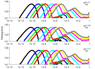
To compare the failure criteria of the surface code between the Pauli error model and pulse-area error model, we perform surface code simulations using the exact same circuit as for the Pauli error model just shown. We use the following error strengths, : 0.0025, 0.005, 0.0075, 0.01, 0.02, 0.03, 0.04, 0.05 ( samples per error rate). Broad, heavy-tailed distributions for the failure criteria are again observed as shown in Fig. 9 and appear to follow a log-normal distribution in a majority of the cases. Once again, just as the failure metrics for the Pauli error model and pulse area error model varied drastically with the Steane code, the surface code displays similar behavior. There is no simple map between the Pauli error model and the pulse area error model, with the pulse-area error model leading to quite broad and heavy-tailed distributions.
VI Conclusions
We have presented a wavefunction simulation of Steane’s [[7,1,3]] quantum error correcting code and the tilted-17 surface code for both the stochastic Pauli error model and the coherent pulse-area error model for randomly encoded states. The usual failure criteria had to be modified in order to account for the different frame that non-stabilizer states occupy. A comparison of Fig. 1 and Fig. 4 shows that the two error models result in markedly different failure distributions. Pauli errors tend to draw down from 1.0 with increasing . These tails empirically vary as . In contrast, for increasing in the pulse-area error model, the distribution rises from small , with the most likely values scaling as . We conjecture that the heavy tails in the pulse-area error model distribution are an indicator of the strongly negative impact that purely coherent errors can have on QEC Sanders et al. (2016); Kueng et al. (2016).
These results also demonstrate that any result attempting to approximate arbitrary physical error channels with stochastic Pauli error channels must do so only when modeling certain system-bath type models. We have shown that one cannot rely on the assumption that syndrome measurements cut off the interfering pathways. A stochastic error model is only appropriate when the source of noise is due only to errors that are entangled with bath states that are mutually orthogonal to all other bath states. Of course, this is not true in general with coherent errors being the extreme counter-example. A simulation employing such an approximation, while it may be able to bound or approximate a mean threshold, will not be able to reproduce the output distribution that contains information from the fully coherent sum of all fault paths. As we have shown here, even for very small perturbations, the coherent addition of these fault paths cause marked differences in the output statistics. This also implies that any analysis that contains a perfect QEC measurement cycle and correction will, by design, cut off these coherent pathways, also corrupting the output statistics.
Finally, we note that these output distributions can be used as a more robust metric for QEC performance than just considering the logical error rate. They would allow one to examine whether ideas to randomize coherent errors, such as randomized compiling Wallman and Emerson (2016) do indeed help by making the errors look more “Pauli” like to QEC. The authors do not expect to see any benefit from randomized compiling as the evolution for a single trajectory would still be completely coherent, but this is a question for further investigation.
Acknowledgements.
We acknowledge useful conversations with Joan Hoffmann and Ken Brown. This project was supported by the Intelligence Advanced Research Projects Activity via Department of Interior National Business Center contract number 2012-12050800010. The U.S. Government is authorized to reproduce and distribute reprints for Governmental purposes notwithstanding any copyright annotation thereon. The views and conclusions contained herein are those of the authors and should not be interpreted as necessarily representing the official policies or endorsements, either expressed or implied, of IARPA, DoI/NBC, or the U.S. Government.References
- Shor (1995) P. W. Shor, Phys. Rev. A 52, R2493 (1995).
- Steane (1996) A. Steane, Physical Review Letters 77, 793 (1996).
- Calderbank and Shor (1996) A. Calderbank and P. Shor, Physical Review A 54, 1098 (1996).
- Aharonov and Ben-Or (1997) D. Aharonov and M. Ben-Or, in Proceedings of the Twenty-ninth Annual ACM Symposium on Theory of Computing, STOC ’97 (ACM, New York, NY, USA, 1997) pp. 176–188.
- Knill et al. (1998) E. Knill, R. Laflamme, and W. H. Zurek, Proceedings of the Royal Society of London A: Mathematical, Physical and Engineering Sciences 454, 365 (1998).
- Aliferis et al. (2006) P. Aliferis, D. Gottesman, and J. Preskill, Quantum Information and Computation 6, 97 (2006).
- Aharonov and Ben-Or (2008) D. Aharonov and M. Ben-Or, “Fault-tolerant quantum computation with constant error rate,” (2008) pp. 1207–1282.
- Gottesman (2010) D. Gottesman, in Quantum Information Science and Its Contributions to Mathematics (Amer. Math. Soc., 2010) pp. 13–58.
- Terhal (2015) B. M. Terhal, Rev. Mod. Phys. 87, 307 (2015).
- Nielsen and Chuang (2010) M. A. Nielsen and I. L. Chuang, Quantum Computation and Quantum Information, 10th ed. (Cambridge University Press, 2010).
- Haake (2001) F. Haake, Quantum Signatures of Chaos, 2nd ed. (Springer, 2001).
- Breuer and Petruccione (2002) H.-P. Breuer and F. Petruccione, The Theory of Open Quantum Systems (Oxford, 2002).
- Weiss (2012) U. Weiss, Quantum Dissipative Systems, 4th ed. (World Scientific, 2012).
- Knill and Laflamme (1996) E. Knill and R. Laflamme, quant-ph/9608012 , 1 (1996).
- Shor (1996) P. W. Shor, in Foundations of Computer Science, 1996. Proceedings., 37th Annual Symposium on (IEEE, 1996) pp. 56–65.
- Sanders et al. (2016) Y. R. Sanders, J. J. Wallman, and B. C. Sanders, New Journal of Physics 18, 012002 (2016).
- Kueng et al. (2016) R. Kueng, D. M. Long, A. C. Doherty, and S. T. Flammia, Phys. Rev. Lett. 117, 170502 (2016).
- Gutiérrez et al. (2013) M. Gutiérrez, L. Svec, A. Vargo, and K. R. Brown, Physical Review A 87, 030302(R) (2013).
- Geller and Zhou (2013) M. R. Geller and Z. Zhou, Physical Review A 88, 012314 (2013).
- Puzzuoli et al. (2014) D. Puzzuoli, C. Granade, H. Haas, B. Criger, E. Magesan, and D. G. Cory, Physical Review A 89, 022306 (2014).
- Witzel et al. (2014) W. M. Witzel, K. Young, and S. D. Sarma, Physical Review B 90, 115431 (2014).
- Darmawan and Poulin (2016) A. S. Darmawan and D. Poulin, arXiv preprint arXiv:1607.06460 (2016).
- Gutiérrez et al. (2016) M. Gutiérrez, C. Smith, L. Lulushi, S. Janardan, and K. R. Brown, Phys. Rev. A 94, 042338 (2016).
- Gottesman (1998) D. Gottesman, arXiv preprint quant-ph/9807006 (1998).
- Aaronson and Gottesman (2004) S. Aaronson and D. Gottesman, Physical Review A 70, 052328 (2004).
- Rahn et al. (2002) B. Rahn, A. C. Doherty, and H. Mabuchi, Phys. Rev. A 66, 032304 (2002).
- Bombin and Martin-Delgado (2007) H. Bombin and M. A. Martin-Delgado, Phys. Rev. A 76, 012305 (2007).
- Horsman et al. (2012) C. Horsman, A. G. Fowler, S. Devitt, and R. V. Meter, New Journal of Physics 14, 123011 (2012).
- Kitaev (2003) A. Kitaev, Annals of Physics 303, 2 (2003).
- Cross et al. (2009) A. Cross, D. P. DiVincenzo, and B. M. Terhal, quant-ph/0711.1556v2 x, 1 (2009).
- Cohen-Tannoudji et al. (1989) C. Cohen-Tannoudji, J. Dupont-Roc, and G. Grynberg, Photons and Atoms (Wiley, 1989).
- Heitler (1954) W. Heitler, The Quantum Theory of Radiation, 3rd ed. (Dover, 1954).
- Ernst et al. (1987) R. Ernst, G. Bodenhausen, and A. Wokaun, Principles of Nuclear Magnetic Resonance in One and Two Dimensions (Oxford, 1987).
- Yariv (1996) A. Yariv, Optical Electronics in Modern Communications, 5th ed. (Oxford, 1996).
- Mandel and Wolf (1995) L. Mandel and E. Wolf, Optical Coherence and Quantum Optics (Cambridge University Press, 1995).
- Barnes and Warren (1999) J. Barnes and W. Warren, Physical Review A 60, 4363 (1999).
- Merrill and Brown (2014) J. T. Merrill and K. R. Brown, “Progress in compensating pulse sequences for quantum computation,” in Quantum Information and Computation for Chemistry (John Wiley and Sons, 2014) pp. 241–294.
- Coherent (2016) Coherent, Coherent Ultrafast Laser Systems 2016 Product Catalog, Vol. 0 (Coherent, 2016) p. 0.
- DiVincenzo and Aliferis (2007) D. P. DiVincenzo and P. Aliferis, Phys. Rev. Lett. 98, 020501 (2007).
- Svore et al. (2006) K. M. Svore, A. W. Cross, I. L. Chuang, and A. V. Aho, Quantum Information and Computation 6, 193 (2006).
- Tomita and Svore (2014) Y. Tomita and K. M. Svore, Phys. Rev. A 90, 062320 (2014).
- Fowler et al. (2012) A. G. Fowler, A. C. Whiteside, and L. C. L. Hollenberg, Phys. Rev. Lett. 108, 180501 (2012).
- Edmonds (1965a) J. Edmonds, Canad. J. Math. 17, 449 (1965a).
- Edmonds (1965b) J. Edmonds, J. Res. Nat. Bur. Standards 69B, 125 (1965b).
- Wallman and Emerson (2016) J. J. Wallman and J. Emerson, Phys. Rev. A 94, 052325 (2016).