Higher-order clustering in networks

Abstract

A fundamental property of complex networks is the tendency for edges to cluster. The extent of the clustering is typically quantified by the clustering coefficient, which is the probability that a length-2 path is closed, i.e., induces a triangle in the network. However, higher-order cliques beyond triangles are crucial to understanding complex networks, and the clustering behavior with respect to such higher-order network structures is not well understood. Here we introduce higher-order clustering coefficients that measure the closure probability of higher-order network cliques and provide a more comprehensive view of how the edges of complex networks cluster. Our higher-order clustering coefficients are a natural generalization of the traditional clustering coefficient. We derive several properties about higher-order clustering coefficients and analyze them under common random graph models. Finally, we use higher-order clustering coefficients to gain new insights into the structure of real-world networks from several domains.

I Introduction

Networks are a fundamental tool for understanding and modeling complex physical, social, informational, and biological systems Newman (2003). Although such networks are typically sparse, a recurring trait of networks throughout all of these domains is the tendency of edges to appear in small clusters or cliques Rapoport (1953); Watts and Strogatz (1998). In many cases, such clustering can be explained by local evolutionary processes. For example, in social networks, clusters appear due to the formation of triangles where two individuals who share a common friend are more likely to become friends themselves, a process known as triadic closure Rapoport (1953); Granovetter (1973). Similar triadic closures occur in other networks: in citation networks, two references appearing in the same publication are more likely to be on the same topic and hence more likely to cite each other Wu and Holme (2009) and in co-authorship networks, scientists with a mutual collaborator are more likely to collaborate in the future Jin et al. (2001). In other cases, local clustering arises from highly connected functional units operating within a larger system, e.g., metabolic networks are organized by densely connected modules Ravasz and Barabási (2003).

The clustering coefficient quantifies the extent to which edges of a network cluster in terms of triangles. The clustering coefficient is defined as the fraction of length-2 paths, or wedges, that are closed with a triangle Watts and Strogatz (1998); Barrat and Weigt (2000) (Fig. 1, row $C_{2}$). In other words, the clustering coefficient measures the probability of triadic closure in the network. However, the clustering coefficient is inherently restrictive as it measures the closure probability of just one simple structure—the triangle. Moreover, higher-order structures such as larger cliques are crucial to the structure and function of complex networks Benson et al. (2016); Yaveroğlu et al. (2014); Rosvall et al. (2014). For example, 4-cliques reveal community structure in word association and protein-protein interaction networks Palla et al. (2005) and cliques of sizes 5–7 are more frequent than triangles in many real-world networks with respect to certain null models Slater et al. (2014). However, the extent of clustering of such higher-order structures has not been well understood nor quantified.

	1. Start with	2. Find an adjacent edge	3. Check for an
	an $\ell$-clique	to form an $\ell$-wedge	$(\ell+1)$-clique
$C_{2}$
$C_{3}$
$C_{4}$

Figure 1: Overview of higher-order clustering coefficients as clique expansion probabilities. The $\ell$th-order clustering coefficient $C_{\ell}$ measures the probability that an $\ell$-clique and an adjacent edge, i.e., an $\ell$-wedge, is closed, meaning that the $\ell-1$ possible edges between the $\ell$-clique and the outside node in the adjacent edge exist to form an $(\ell+1)$-clique.

Here, we provide a framework to quantify higher-order clustering in networks by measuring the normalized frequency at which higher-order cliques are closed, which we call higher-order clustering coefficients. We derive our higher-order clustering coefficients by extending a novel interpretation of the classical clustering coefficient as a form of clique expansion (Fig. 1). We then derive several properties about higher-order clustering coefficients and analyze them under the $G_{n,p}$ and small-world null models.

Using our theoretical analysis as a guide, we analyze the higher-order clustering behavior of real-world networks from a variety of domains. We find that each domain of networks has its own higher-order clustering pattern, which the traditional clustering coefficient does not show on its own. Conventional wisdom in network science posits that practically all real-world networks exhibit clustering; however, we find that not all networks exhibit higher-order clustering. More specifically, once we control for the clustering as measured by the classical clustering coefficient, some networks do not show significant clustering in terms of higher-order cliques. In addition to the theoretical properties and empirical findings exhibited in this paper, our related work also demonstrates a connection between higher-order clustering and community detection Yin et al. (2017).

II Derivation of higher-order clustering coefficients

In this section, we derive our higher-order clustering coefficients and some of their basic properties. We first present an alternative interpretation of the classical clustering coefficient and then show how this novel interpretation seamlessly generalizes to arrive at our definition of higher-order clustering coefficients. We then provide some probabilistic interpretations of higher-order clustering coefficients that will be useful for our subsequent analysis.

II.1 Alternative interpretation of the classical clustering coefficient

Here we give an alternative interpretation of the clustering coefficient that will later allow us to generalize it and quantify clustering of higher-order network structures (this interpretation is summarized in Fig. 1). Our interpretation is based on a notion of clique expansion. First, we consider a $2$-clique $K$ in a graph $G$ (that is, a single edge $K$; see Fig. 1, row $C_{2}$, column 1). Next, we expand the clique $K$ by considering any edge $e$ adjacent to $K$, i.e., $e$ and $K$ share exactly one node (Fig. 1, row $C_{2}$, column 2). This expanded subgraph forms a wedge, i.e., a length-$2$ path. The classical global clustering coefficient $C$ of $G$ (sometimes called the transitivity of $G$ Boccaletti et al. (2006)) is then defined as the fraction of wedges that are closed, meaning that the $2$-clique and adjacent edge induce a $(2+1)$-clique, or a triangle (Fig. 1, row $C_{2}$, column 3) Barrat and Weigt (2000); Luce and Perry (1949). The novelty of our interpretation of the clustering coefficient is considering it as a form of clique expansion, rather than as the closure of a length-$2$ path, which is key to our generalizations in the next section.

Formally, the classical global clustering coefficient is

$$C=\frac{6\lvert K_{3}\rvert}{\lvert W\rvert},$$ (1)

where $K_{3}$ is the set of $3$-cliques (triangles), $W$ is the set of wedges, and the coefficient $6$ comes from the fact that each $3$-clique closes 6 wedges—the 6 ordered pairs of edges in the triangle.

We can also reinterpret the local clustering coefficient Watts and Strogatz (1998) in this way. In this case, each wedge again consists of a $2$-clique and adjacent edge (Fig. 1, row $C_{2}$, column 2), and we call the unique node in the intersection of the $2$-clique and adjacent edge the center of the wedge. The local clustering clustering coefficient of a node $u$ is the fraction of wedges centered at $u$ that are closed:

$$C(u)=\dfrac{2\lvert K_{3}(u)\rvert}{\lvert W(u)\rvert},$$ (2)

where $K_{3}(u)$ is the set of $3$-cliques containing $u$ and $W(u)$ is the set of wedges with center $u$ (if $\lvert W(u)\rvert=0$, we say that $C(u)$ is undefined). The average clustering coefficient $\bar{C}$ is the mean of the local clustering coefficients,

$$\bar{C}=\frac{1}{\lvert\widetilde{V}\rvert}\sum_{u\in\widetilde{V}}C(u),$$ (3)

where $\widetilde{V}$ is the set of nodes in the network where the local clustering coefficient is defined.

II.2 Generalizing to higher-order clustering coefficients

Our alternative interpretation of the clustering coefficient, described above as a form of clique expansion, leads to a natural generalization to higher-order cliques. Instead of expanding $2$-cliques to $3$-cliques, we expand $\ell$-cliques to $(\ell+1)$-cliques (Fig. 1, rows $C_{3}$ and $C_{4}$). Formally, we define an $\ell$-wedge to consist of an $\ell$-clique and an adjacent edge for $\ell\geq 2$. Then we define the global $\ell$th-order clustering coefficient $C_{\ell}$ as the fraction of $\ell$-wedges that are closed, meaning that they induce an $(\ell+1)$-clique in the network. We can write this as

$$C_{\ell}=\frac{(\ell^{2}+\ell)\lvert K_{\ell+1}\rvert}{\lvert W_{\ell}\rvert},$$ (4)

where $K_{\ell+1}$ is the set of $(\ell+1)$-cliques, and $W_{\ell}$ is the set of $\ell$-wedges. The coefficient $\ell^{2}+\ell$ comes from the fact that each $(\ell+1)$-clique closes that many wedges: each $(\ell+1)$-clique contains $\ell+1$ $\ell$-cliques, and each $\ell$-clique contains $\ell$ nodes which may serve as the center of an $\ell$-wedge. Note that the classical definition of the global clustering coefficient given in Eq. 1 is equivalent to the definition in Eq. 4 when $\ell=2$.

We also define higher-order local clustering coefficients:

$$C_{\ell}(u)=\frac{\ell\lvert K_{\ell+1}(u)\rvert}{\lvert W_{\ell}(u)\rvert},$$ (5)

where $K_{\ell+1}(u)$ is the set of $(\ell+1)$-cliques containing node $u$, $W_{\ell}(u)$ is the set of $\ell$-wedges with center $u$ (where the center is the unique node in the intersection of the $\ell$-clique and adjacent edge comprising the wedge; see Fig. 1), and the coefficient $\ell$ comes from the fact that each $(\ell+1)$-clique containing $u$ closes that many $\ell$-wedges in $W_{\ell}(u)$. The $\ell$th-order clustering coefficient of a node is defined for any node that is the center of at least one $\ell$-wedge, and the average $\ell$th-order clustering coefficient is the mean of the local clustering coefficients:

$$\bar{C}_{\ell}=\frac{1}{\lvert\widetilde{V}_{\ell}\rvert}\sum_{u\in\widetilde{V}_{\ell}}C_{\ell}(u),$$ (6)

where $\widetilde{V}_{\ell}$ is the set of nodes that are the centers of at least one $\ell$-wedge.

To understand how to compute higher-order clustering coefficients, we substitute the following useful identity

$$\lvert W_{\ell}(u)\rvert=\lvert K_{\ell}(u)\rvert\cdot(d_{u}-\ell+1),$$ (7)

where $d_{u}$ is the degree of node $u$, into Eq. 5 to get

$$C_{\ell}(u)=\frac{\ell\cdot\lvert K_{\ell+1}(u)\rvert}{(d_{u}-\ell+1)\cdot\lvert K_{\ell}(u)\rvert}.$$ (8)

From Eq. 8, it is easy to see that we can compute all local $\ell$th-order clustering coefficients by enumerating all $(\ell+1)$-cliques and $\ell$-cliques in the graph. The computational complexity of the algorithm is thus bounded by the time to enumerate $(\ell+1)$-cliques and $\ell$-cliques. Using the Chiba and Nishizeki algorithm Chiba and Nishizeki (1985), the complexity is $O(\ell a^{\ell-2}m)$, where $a$ is the arboricity of the graph, and $m$ is the number of edges. The arboricity $a$ may be as large as $\sqrt{m}$, so this algorithm is only guaranteed to take polynomial time if $\ell$ is a constant. In general, determining if there exists a single clique with at least $\ell$ nodes is NP-complete Karp (1972).

For the global clustering coefficient, note that

$$\lvert W_{\ell}\rvert=\sum_{u\in V}\lvert W_{\ell}(u)\rvert.$$ (9)

Thus, it suffices to enumerate $\ell$-cliques (to compute $\lvert W_{\ell}\rvert$ using Eq. 7) and to count the total number of $\ell$-cliques. In practice, we use the Chiba and Nishizeki to enumerate cliques and simultaneously compute $C_{\ell}$ and $C_{\ell}(u)$ for all nodes $u$. This suffices for our clustering analysis with $\ell=2,3,4$ on networks with over a hundred million edges in Section IV.

II.3 Probabilistic interpretations of higher-order clustering coefficients

To facilitate understanding of higher-order clustering coefficients and to aid our analysis in Section III, we present a few probabilistic interpretations of the quantities. First, we can interpret $C_{\ell}(u)$ as the probability that a wedge $w$ chosen uniformly at random from all wedges centered at $u$ is closed:

$$C_{\ell}(u)=\mbox{$\mathbb{P}$}\left[w\in K_{\ell+1}(u)\right].$$ (10)

The variant of this interpretation for the classical clustering case of $\ell=2$ has been useful for graph algorithm development Seshadhri et al. (2013).

For the next probabilistic interpretation, it is useful to analyze the structure of the 1-hop neighborhood graph $N_{1}(u)$ of a given node $u$ (not containing node $u$). The vertex set of $N_{1}(u)$ is the set of all nodes adjacent to $u$, and the edge set consists of all edges between neighbors of $u$, i.e., $\{(v,w)\;|\;(u,v),(u,w),(v,w)\in E\}$, where $E$ is the edge set of the graph.

Any $\ell$-clique in $G$ containing node $u$ corresponds to a unique $(\ell-1)$-clique in $N_{1}(u)$, and specifically for $\ell=2$, any edge $(u,v)$ corresponds to a node $v$ in $N_{1}(u)$. Therefore, each $\ell$-wedge centered at $u$ corresponds to an $(\ell-1)$-clique $K$ and one of the $d_{u}-\ell+1$ nodes outside $K$ (i.e., in $N_{1}(u)\backslash K$). Thus, Eq. 8 can be re-written as

$$\frac{\ell\cdot\lvert K_{\ell}(N_{1}(u))\rvert}{(d_{u}-\ell+1)\cdot\lvert K_{\ell-1}(N_{1}(u))\rvert},$$ (11)

where $K_{k}(N_{1}(u))$ denotes the number of $k$-cliques in $N_{1}(u)$.

If we uniformly at random select an $(\ell-1)$-clique $K$ from $N_{1}(u)$ and then also uniformly at random select a node $v$ from $N_{1}(u)$ outside of this clique, then $C_{\ell}(u)$ is the probability that these $\ell$ nodes form an $\ell$-clique:

$$C_{\ell}(u)=\mbox{$\mathbb{P}$}\left[K\cup\{v\}\in K_{\ell}(N_{1}(u))\right].$$ (12)

Moreover, if we condition on observing an $\ell$-clique from this sampling procedure, then the $\ell$-clique itself is selected uniformly at random from all $\ell$-cliques in $N_{1}(u)$. Therefore, $C_{\ell-1}(u)\cdot C_{\ell}(u)$ is the probability that an $(\ell-1)$-clique and two nodes selected uniformly at random from $N_{1}(u)$ form an $(\ell+1)$-clique. Applying this recursively gives

$$\prod_{j=2}^{\ell}C_{j}(u)=\frac{\lvert K_{\ell}(N_{1}(u))\rvert}{{d_{u}\choose\ell}}.$$ (13)

In other words, the product of the higher-order local clustering coefficients of node $u$ up to order $\ell$ is the $\ell$-clique density amongst $u$’s neighbors.

III Theoretical analysis and higher-order clustering in random graph models

We now provide some theoretical analysis of our higher-order clustering coefficients. We first give some extremal bounds on the values that higher-order clustering coefficients can take given the value of the traditional (second-order) clustering coefficient. After, we analyze the values of higher-order clustering coefficients in two common random graph models—the $G_{n,p}$ and small-world models. The theory from this section will be a useful guide for interpreting the clustering behavior of real-world networks in Section IV.

III.1 Extremal bounds

$C_{2}(u)$	$1$	$\dfrac{d}{2(d-1)}\approx\dfrac{1}{2}$	$\frac{d-2}{4d-4}\approx\dfrac{1}{4}$
$C_{3}(u)$	$1$	$0$	$\dfrac{d-4}{2d-4}\approx\dfrac{1}{2}$
$C_{4}(u)$	$1$	$0$	$\dfrac{d-6}{2d-6}\approx\dfrac{1}{2}$

Figure 2: Example 1-hop neighborhoods of a node $u$ with degree $d$ with different higher-order clustering. Left: For cliques, $C_{\ell}(u)=1$ for any $\ell$. Middle: If $u$’s neighbors form a complete bipartite graph, $C_{2}(u)$ is constant while $C_{\ell}(u)=0$, $\ell\geq 3$. Right: If half of $u$’s neighbors form a star and half form a clique with $u$, then $C_{\ell}(u)\approx\sqrt{C_{2}(u)}$, which is the upper bound in Proposition 1.

We first analyze the relationships between local higher-order clustering coefficients of different orders. Our technical result is Proposition 1, which provides essentially tight lower and upper bounds for higher-order local clustering coefficients in terms of the traditional local clustering coefficient. The main ideas of the proof are illustrated in Fig. 2.

Proposition 1.

For any fixed $\ell\geq 3$,

$$0\leq C_{\ell}(u)\leq\sqrt{C_{2}(u)}.$$ (14)

Moreover,

1. There exists a finite graph $G$ with a node $u$ such that the lower bound is tight and $C_{2}(u)$ is within $\epsilon$ of any prescribed value in $[0,\frac{\ell-2}{\ell-1}]$.

2. There exists a finite graph $G$ with a node $u$ such that $C_{\ell}(u)$ is within $\epsilon$ of the upper bound for any prescribed value of $C_{2}(u)\in[0,1]$.

Proof.

Clearly, $0\leq C_{\ell}(u)$ if the local clustering coefficient is well defined. This bound is tight when $N_{1}(u)$ is $(\ell-1)$-partite, as in the middle column of Fig. 2. In the $(\ell-1)$-partite case, $C_{2}(u)=\frac{\ell-2}{\ell-1}$. By removing edges from this extremal case in a sufficiently large graph, we can make $C_{2}(u)$ arbitrarily close to any value in $[0,\frac{\ell-2}{\ell-1}]$.

To derive the upper bound, consider the 1-hop neighborhood $N_{1}(u)$, and let

$$\delta_{\ell}(N_{1}(u))=\frac{\lvert K_{\ell}(N_{1}(u))\rvert}{{d_{u}\choose\ell}}$$ (15)

denote the $\ell$-clique density of $N_{1}(u)$. The Kruskal-Katona theorem Kruskal (1963); Katona (1966) implies that

$$\delta_{\ell}(N_{1}(u))\leq[\delta_{\ell-1}(N_{1}(u))]^{\ell/(\ell-1)}$$

$$\delta_{\ell-1}(N_{1}(u))\leq[\delta_{2}(N_{1}(u))]^{(\ell-1)/2}.$$

Combining this with Eq. 8 gives

$$C_{\ell}(u) \leq[\delta_{\ell-1}(N_{1}(u))]^{\frac{1}{\ell-1}}\leq\sqrt{\delta_{2}(N_{1}(u))}=\sqrt{C_{2}(u)},$$

where the last equality uses the fact that $C_{2}(u)$ is the edge density of $N_{1}(u)$.

The upper bound becomes tight when $N_{1}(u)$ consists of a clique and isolated nodes (Fig. 2, right) and the neighborhood is sufficiently large. Specifically, let $N_{1}(u)$ consist of a clique of size $c$ and $b$ isolated nodes. When $\ell=2$,

$$C_{\ell}(u)=\frac{{c\choose 2}}{{c+b\choose 2}}=\frac{(c-1)c}{(c+b-1)(c+b)}\to\left(\frac{c}{c+b}\right)^{2}$$

and by Eq. 11, when $3\leq\ell\leq c$,

$$C_{\ell}(u) =\frac{\ell\cdot{c\choose\ell}}{(c+b-\ell+1)\cdot{c\choose\ell-1}}=\frac{c-\ell+1}{c+b-\ell+1}\to\frac{c}{c+b}.$$

By adjusting the ratio $c/(b+c)$ in $N_{1}(u)$, we can construct a family of graphs such that $C_{2}(u)$ takes any value in the interval $[0,1]$ as $d_{u}\to\infty$ and $C_{\ell}(u)\to\sqrt{C_{2}(u)}$ as $d_{u}\to\infty$. ∎

The second part of the result requires the neighborhoods to be sufficiently large in order to reach the upper bound. However, we will see later that in some real-world data, there are nodes $u$ for which $C_{3}(u)$ is close to the upper bound $\sqrt{C_{2}(u)}$ for several values of $C_{2}(u)$.

Next, we analyze higher-order clustering coefficients in two common random graph models: the Erdős-Rényi model with edge probability $p$ (i.e., the $G_{n,p}$ model Erdös and Rényi (1959)) and the small-world model Watts and Strogatz (1998).

III.2 Analysis for the $G_{n,p}$ model

Now, we analyze higher-order clustering coefficients in classical Erdős-Rényi random graph model, where each edge exists independently with probability $p$ (i.e., the $G_{n,p}$ model Erdös and Rényi (1959)). We implicitly assume that $\ell$ is small in the following analysis so that there should be at least one $\ell$-wedge in the graph (with high probability and $n$ large, there is no clique of size greater than $(2+\epsilon)\log n/\log(1/p)$ for any $\epsilon>0$ Bollobás and Erdös (1976)). Therefore, the global and local clustering coefficients are well-defined.

In the $G_{n,p}$ model, we first observe that any $\ell$-wedge is closed if and only if the $\ell-1$ possible edges between the $\ell$-clique and the outside node in the adjacent edge exist to form an $(\ell+1)$-clique. Each of the $\ell-1$ edges exist independently with probability $p$ in the $G_{n,p}$ model, which means that the higher-order clustering coefficients should scale as $p^{\ell-1}$. We formalize this in the following proposition.

Proposition 2.

Let $G$ be a random graph drawn from the $G_{n,p}$ model. For constant $\ell$,

1. $\mbox{$\mathbb{E}_{G}$}\left[C_{\ell}\right]=p^{\ell-1}$

2. $\mbox{$\mathbb{E}_{G}$}\left[C_{\ell}(u)\;|\;W_{\ell}(u)>0\right]=p^{\ell-1}$ for any node $u$

3. $\mbox{$\mathbb{E}_{G}$}\left[\bar{C}_{\ell}\right]=p^{\ell-1}$

Proof.

We prove the first part by conditioning on the set of $\ell$-wedges, $W_{\ell}$:

$$\mbox{$\mathbb{E}$}[C_{\ell}] =\textstyle\mbox{$\mathbb{E}_{G}$}\left[\mbox{$\mathbb{E}_{W_{\ell}}$}\left[C_{\ell}\;|\;W_{\ell}\right]\right]$$

$$=\textstyle\mbox{$\mathbb{E}_{G}$}\left[\mbox{$\mathbb{E}_{W_{\ell}}$}\left[\frac{1}{\lvert W_{\ell}\rvert}\sum_{w\in W_{\ell}}\mbox{$\mathbb{P}$}\left[w\text{ is closed}\right]\right]\right]$$

$$=\textstyle\mbox{$\mathbb{E}_{G}$}\left[\mbox{$\mathbb{E}_{W_{\ell}}$}\left[\frac{1}{\lvert W_{\ell}\rvert}\sum_{w\in W_{\ell}}p^{\ell-1}\right]\right]$$

$$=\textstyle\mbox{$\mathbb{E}_{G}$}\left[p^{\ell-1}\right]$$

$$=\textstyle p^{\ell-1}.$$

As noted above, the second equality is well defined (with high probability) for small $\ell$. The third equality comes from the fact that any $\ell$-wedge is closed if and only if the $\ell-1$ possible edges between the $\ell$-clique and the outside node in the adjacent edge exist to form an $(\ell+1)$-clique.

The proof of the second part is essentially the same, except we condition over the set of possible cases where $W_{\ell}(u)>0$.

Recall that $\widetilde{V}$ is the set of nodes at the center of at least one $\ell$-wedge. To prove the third part, we take the conditional expectation over $\widetilde{V}$ and use our result from the second part. ∎

The above results say that the global, local, and average $\ell$th order clustering coefficients decrease exponentially in $\ell$. It turns out that if we also condition on the second-order clustering coefficient having some fixed value, then the higher-order clustering coefficients still decay exponentially in $\ell$ for the $G_{n,p}$ model. This will be useful for interpreting the distribution of local clustering coefficients on real-world networks.

Proposition 3.

Let $G$ be a random graph drawn from the $G_{n,p}$ model. Then for constant $\ell$,

$$\mbox{$\mathbb{E}_{G}$}\left[C_{\ell}(u)\;|\;C_{2}(u),W_{\ell}(u)>0\right]$$

$$=\left[C_{2}(u)-(1-C_{2}(u))\cdot O(1/d_{u}^{2})\right]^{\ell-1}\approx(C_{2}(u))^{\ell-1}.$$

Proof.

Similar to the proof of Proposition 3, we look at the conditional expectation over $W_{\ell}(u)>0$:

$$\textstyle\mbox{$\mathbb{E}_{G}$}\left[C_{\ell}(u)\;|\;C_{2}(u),W_{\ell}(u)>0\right]$$

$$=\textstyle\mbox{$\mathbb{E}_{G}$}\left[\mbox{$\mathbb{E}_{W_{\ell}(u)>0}$}\left[C_{\ell}(u)\;|\;C_{2}(u),\;W_{\ell}(u)\right]\right]$$

$$=\textstyle\mbox{$\mathbb{E}_{G}$}\left[\mbox{$\mathbb{E}_{W_{\ell}(u)>0}$}\left[\frac{1}{\lvert W_{\ell}(u)\rvert}\sum_{w\in W_{\ell}(u)}\mbox{$\mathbb{P}$}\left[w\text{ closed}\;|\;C_{2}(u)\right]\right]\right].$$

Now, note that $N_{1}(u)$ has $m=C_{2}(u)\cdot{d_{u}\choose 2}$ edges. Knowing that $w\in W_{\ell}(u)$ accounts for ${\ell-1\choose 2}$ of these edges. By symmetry, the other $q=m-{\ell-1\choose 2}$ edges appear in any of the remaining $r={d_{u}\choose 2}-{\ell-1\choose 2}$ pairs of nodes uniformly at random. There are ${r\choose q}$ ways to place these edges, of which ${r-\ell+1\choose q-\ell+1}$ would close the wedge $w$. Thus,

$$\mbox{$\mathbb{P}$}\left[w\text{ is closed}\;|\;C_{2}(u)\right]$$

$$=\textstyle\frac{{r-\ell+1\choose q-\ell+1}}{{r\choose q}}=\frac{(r-\ell+1)!q!}{(q-\ell+1)!r!}=\frac{(q-\ell+2)(q-\ell+3)\cdots q}{(r-\ell+2)(r-\ell+3)\cdots r}.$$

Now, for any small nonnegative integer $k$,

$$\frac{q-k}{r-k} =\textstyle\frac{C_{2}(u)\cdot{d_{u}\choose 2}-{\ell-1\choose 2}-k}{{d_{u}\choose 2}-{\ell-1\choose 2}-k}$$

$$=\textstyle C_{2}(u)-(1-C_{2}(u))\left[\frac{{\ell-1\choose 2}+k}{{d_{u}\choose 2}-{\ell-1\choose 2}-k}\right]$$

$$=\textstyle C_{2}(u)-(1-C_{2}(u))\cdot O(1/d_{u}^{2}).$$

(Recall that $\ell$ is constant by assumption, so the big-O notation is appropriate). The above expression approaches $(C_{2}(u))^{\ell-1}$ when $C_{2}(u)\to 1$ as well as when $d_{u}\to\infty$. ∎

Proposition 3 says that even if the second-order local clustering coefficient is large, the $\ell$th-order clustering coefficient will still decay exponentially in $\ell$, at least in the limit as $d_{u}$ grows large. By examining higher-order clique closures, this allows us to distinguish between nodes $u$ whose neighborhoods are “dense but random” ($C_{2}(u)$ is large but $C_{\ell}(u)\approx(C_{2}(u))^{\ell-1}$) or “dense and structured” ($C_{2}(u)$ is large and $C_{\ell}(u)>(C_{2}(u))^{\ell-1}$). Only the latter case exhibits higher-order clustering. We use this in our analysis of real-world networks in Section IV.

III.3 Analysis for the small-world model

We also study higher-order clustering in the small-world random graph model Watts and Strogatz (1998). The model begins with a ring network where each node connects to its $2k$ nearest neighbors. Then, for each node $u$ and each of the $k$ edges $(u,v)$ with $v$ following $u$ clockwise in the ring, the edge is rewired to $(u,w)$ with probability $p$, where $w$ is chosen uniformly at random.

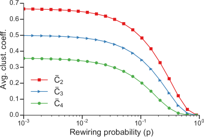
Figure 3: Average higher-order clustering coefficient $\bar{C}_{\ell}$ as a function of rewiring probability $p$ in small-world networks for $\ell=2,3,4$ ($n=20,000$, $k=5$). Proposition 4 shows that the $\ell$th-order clustering coefficient when $p=0$ predicts that the clustering should decrease modestly as $\ell$ increases.

With no rewiring ($p=0$) and $k\ll n$, it is known that $\bar{C}_{2}\approx 3/4$ Watts and Strogatz (1998). As $p$ increases, the average clustering coefficient $\bar{C}_{2}$ slightly decreases until a phase transition near $p=0.1$, where $\bar{C}_{2}$ decays to $0$ Watts and Strogatz (1998) (also see Fig. 3). Here, we generalize these results for higher-order clustering coefficients.

Proposition 4.

In the small-world model without rewiring ($p=0$),

$$\bar{C}_{\ell}\rightarrow(\ell+1)/(2\ell)$$

for any constant $\ell\geq 2$ as $k\to\infty$ and $n\to\infty$ while $2k<n$.

Proof.

Applying Eq. 8, it suffices to show that

$$\lvert K_{\ell}(u)\rvert=\frac{\ell}{(\ell-1)!}\cdot k^{\ell-1}+O(k^{\ell-2})$$ (16)

as

$$C_{\ell}(u)=\frac{\ell\cdot\frac{(\ell+1)k^{\ell}}{\ell!}}{(2k-\ell+1)\cdot\frac{\ell k^{\ell-1}}{(\ell-1)!}},$$

which approaches $\frac{\ell+1}{2\ell}$ as $k\to\infty$.

Now we give a derivation of Eq. 16. We first label the $2k$ neighbors of $u$ as $1,2,\ldots,2k$ by their clockwise ordering in the ring. Since $2k<n$, these nodes are unique. Next, define the span of any $\ell$-clique containing $u$ as the difference between the largest and smallest label of the $\ell-1$ nodes in the clique other than $u$. The span $s$ of any $\ell$-clique satisfies $s\leq k-1$ since any node is directly connected with a node of label difference no greater than $k-1$. Also, $s\geq\ell-2$ since there are $\ell-1$ nodes in an $\ell$-clique other than $u$. For each span $s$, we can find $2k-1-s$ pairs of $(i,j)$ such that $1\leq i$, $j\leq 2k$ and $j-i=s$. Finally, for every such pair $(i,j)$, there are ${s-1\choose\ell-3}$ choices of $\ell-3$ nodes between $i$ and $j$ which will form an $\ell$-clique together with nodes $u$, $i$, and $j$. Therefore,

$$\lvert K_{\ell}(u)\rvert =\textstyle\sum_{s=\ell-2}^{k-1}(2k-1-s)\cdot{s-1\choose\ell-3}$$

$$=\textstyle\sum_{s=\ell-2}^{k-1}(2k-1-s)\cdot\frac{(s-1)(s-2)\cdots(s-\ell+3)}{(\ell-3)!}$$

$$=\textstyle\sum_{t=1}^{k-\ell+2}(2k+2-t-\ell)\cdot\frac{t(t+1)\cdots(t+\ell-4)}{(\ell-3)!}.$$

If we ignore lower-order terms $k$ and note that $t=O(k)$, we get

$$\textstyle\lvert K_{\ell}(u)\rvert =\textstyle\sum_{t=1}^{k}\left[\frac{(2k-t)t^{\ell-3}}{(\ell-3)!}+O(k^{\ell-3})\right]$$

$$=\textstyle\frac{1}{(\ell-3)!}\sum_{t=1}^{k}(2kt^{\ell-3}-t^{\ell-2})+O(k^{\ell-2}).$$

$$=\textstyle\frac{1}{(\ell-3)!}\left[2k\cdot\frac{k^{\ell-2}}{\ell-2}-\frac{k^{\ell-1}}{\ell-1}\right]+O(k^{\ell-2}),$$

$$=\textstyle\frac{\ell}{(\ell-1)!}\cdot k^{\ell-1}+O(k^{\ell-2}).$$

∎

Proposition 4 shows that, when $p=0$, $\bar{C}_{\ell}$ decreases as $\ell$ increases. Furthermore, via simulation, we observe the same behavior as for $\bar{C}_{2}$ when adjusting the rewiring probability $p$ (Fig. 3). Regardless of $\ell$, the phase transition happens near $p=0.1$. Essentially, once there is enough rewiring, all local clique structure is lost, and clustering at all orders is lost. This is partly a consequence of Proposition 1, which says that $C_{\ell}(u)\to 0$ as $C_{2}(u)\to 0$ for any $\ell$.

IV Experimental results on real-world networks

We now analyze the higher-order clustering of real-world networks. We first study how the higher-order global and average clustering coefficients vary as we increase the order $\ell$ of the clustering coefficient on a collection of 20 networks from several domains. After, we concentrate on a few representative networks and compare the higher-order clustering of real-world networks to null models. We find that only some networks exhibit higher-order clustering once the traditional clustering coefficient is controlled. Finally, we examine the local clustering of real-world networks.

IV.1 Higher-order global and average clustering

Network	Nodes	Edges	$C_{2}$	$C_{3}$	$C_{4}$	$\bar{C}_{2}$	$\bar{C}_{3}$	$\bar{C}_{4}$	$\lvert\widetilde{V}_{2}\rvert/\lvert V\rvert$	$\lvert\widetilde{V}_{3}\rvert/\lvert V\rvert$	$\lvert\widetilde{V}_{4}\rvert/\lvert V\rvert$
Erdős-Rényi Erdös and Rényi (1959)	1,000	99,831	0.200	0.040	0.008	0.200	0.040	0.008	1.000	1.000	1.000
Small-world Watts and Strogatz (1998)	20,000	100,000	0.480	0.359	0.229	0.489	0.350	0.205	1.000	1.000	0.999
P. pacificus Bumbarger et al. (2013)	50	576	0.015	0.051	0.035	0.073	0.052	0.034	0.880	0.580	0.440
C. elegans Watts and Strogatz (1998)	297	2,148	0.181	0.080	0.056	0.308	0.137	0.062	0.949	0.926	0.808
Drosophila-medulla Takemura et al. (2013)	1,781	32,311	0.000	0.002	0.001	0.116	0.061	0.024	0.803	0.616	0.425
mouse-retina Helmstaedter et al. (2013)	1,076	577,350	0.008	0.038	0.029	0.033	0.100	0.085	0.998	0.996	0.994
fb-Stanford Traud et al. (2012)	11,621	568,330	0.157	0.107	0.116	0.253	0.181	0.157	0.955	0.922	0.877
fb-Cornell Traud et al. (2012)	18,660	790,777	0.136	0.106	0.121	0.225	0.169	0.148	0.973	0.951	0.923
Pokec Takac and Zabovsky (2012)	1,632,803	22,301,964	0.047	0.044	0.046	0.122	0.084	0.061	0.900	0.675	0.508
Orkut Mislove et al. (2007)	3,072,441	117,185,083	0.041	0.022	0.019	0.170	0.131	0.110	0.978	0.949	0.878
arxiv-HepPh Leskovec et al. (2007)	12,008	118,505	0.659	0.749	0.788	0.698	0.586	0.519	0.876	0.723	0.567
arxiv-AstroPh Leskovec et al. (2007)	18,772	198,050	0.318	0.326	0.359	0.677	0.609	0.561	0.932	0.839	0.740
congress-committees Porter et al. (2005)	871	248,848	0.037	0.080	0.063	0.082	0.142	0.126	1.000	1.000	1.000
DBLP Yang and Leskovec (2015)	317,080	1,049,866	0.306	0.634	0.821	0.732	0.613	0.517	0.864	0.675	0.489
email-Enron-core Klimt and Yang (2004)	148	1356	0.383	0.245	0.192	0.496	0.363	0.277	0.966	0.946	0.946
email-Eu-core Yin et al. (2017); Leskovec et al. (2007)	1005	16064	0.267	0.170	0.135	0.450	0.329	0.264	0.887	0.847	0.784
CollegeMsg Panzarasa et al. (2009)	1,899	41,579	0.004	0.005	0.003	0.053	0.017	0.006	0.829	0.591	0.332
wiki-Talk Leskovec et al. (2010)	2,394,385	4,659,565	0.002	0.011	0.010	0.201	0.081	0.051	0.262	0.077	0.027
oregon2-010526 Leskovec et al. (2005)	11,461	32,730	0.037	0.085	0.097	0.494	0.294	0.300	0.711	0.269	0.121
as-caida-20071105 Leskovec et al. (2005)	26,475	53,381	0.007	0.012	0.015	0.333	0.159	0.134	0.625	0.171	0.060
p2p-Gnutella31 Ripeanu et al. (2002); Leskovec et al. (2007)	62,586	147,892	0.004	0.003	0.000	0.010	0.001	0.000	0.542	0.067	0.001
as-skitter Leskovec et al. (2005)	1,696,415	11,095,298	0.005	0.007	0.011	0.296	0.126	0.109	0.871	0.633	0.335

Table 1: Higher-order clustering coefficients on random graph models, neural connections, online social networks, collaboration networks, human communication, and technological systems. Broadly, networks from the same domain have similar higher-order clustering characteristics. Since $\widetilde{V}_{\ell}$ is the set of nodes at the center of at least one $\ell$-wedge (see Eq. 6), $\lvert\widetilde{V}_{\ell}\rvert/\lvert V\rvert$ is the fraction of nodes at the center of at least one $\ell$-wedge (the higher-order average clustering coefficient $\bar{C}_{\ell}$ is only measured over those nodes participating in at least one $\ell$-wedge).

We compute and analyze the higher-order clustering for networks from a variety of domains (Table 1). We briefly describe the collection of networks and their categorization below:

1. Two synthetic networks—a random instance of an Erdős-Rényi graph with $n=1,000$ nodes and edge probability $p=0.2$ and a small-world network with $n=20,000$ nodes, $k=10$, and rewiring probability $p=0.1$;

2. Four neural networks—the complete neural systems of the nematode worms P. pacificus and C. elegans as well as the neural connections of the Drosophila medulla and mouse retina;

3. Four online social networks—two Facebook friendship networks between students at universities from 2005 (fb-Stanford, fb-Cornell) and two complete online friendship networks (Pokec and Orkut);

4. Four collaboration networks—two co-authorship networks constructed from arxiv submission categories (arxiv-AstroPh and arxiv-HepPh), a co-authorship network constructed from DBLP, and the co-committee membership network of United States congresspersons (congress-committees);

5. Four human communication networks—two email networks (email-Enron-core, email-Eu-core), a Facebook-like messaging network from a college (CollegeMsg), and the edits of user talk pages by other users on Wikipedia (wiki-Talk); and

6. Four technological systems networks—three autonomous systems (oregon2-010526, as-caida-20071105, as-skitter) and a peer-to-peer connection network (p2p-Genutella31).

In all cases, we take the edges as undirected, even if the original network data is directed.

Table 1 lists the $\ell$th-order global and average clustering coefficients for $\ell=2,3,4$ as well as the fraction of nodes that are the center of at least one $\ell$-wedge (recall that the average clustering coefficient is the mean only over higher-order local clustering coefficients of nodes participating in at least one $\ell$-wedge; see Kaiser (2008) for a discussion on how this can affect network analyses). We highlight some important trends in the raw clustering coefficients, and in the next section, we focus on higher-order clustering compared to what one gets in a null model.

Propositions 2 and 4 say that we should expect the higher-order global and average clustering coefficients to decrease as we increase the order $\ell$ for both the Erdős-Rényi and small-world models, and indeed $\bar{C}_{2}>\bar{C}_{3}>\bar{C}_{4}$ for these networks. This trend also holds for most of the real-world networks (mouse-retina, congress-committees, and oregon2-010526 are the exceptions). Thus, when averaging over nodes, higher-order cliques are overall less likely to close in both the synthetic and real-world networks.

C. elegans

fb-Stanford

arxiv-AstroPh

email-Enron-core

oregon2-010526

original

CM

MRCN

original

CM

MRCN

original

CM

MRCN

original

CM

MRCN

original

CM

MRCN

$\bar{C}_{2}$

$0.31$

$0.15^{\ast}$

$0.31\phantom{{}^{\ast}}$

$0.25$

$0.03^{\ast}$

$0.25\phantom{{}^{\ast}}$

$0.68$

$0.01^{\ast}$

$0.68\phantom{{}^{\ast}}$

$0.50$

$0.23^{\ast}$

$0.50\phantom{{}^{\ast}}$

$0.49$

$0.25^{\ast}$

$0.49\phantom{{}^{\ast}}$

$\bar{C}_{3}$

$0.14$

$0.04^{\ast}$

$0.17^{\dagger}$

$0.18$

$0.00^{\ast}$

$0.14^{\ast}$

$0.61$

$0.00^{\ast}$

$0.60\phantom{{}^{\ast}}$

$0.36$

$0.08^{\ast}$

$0.35\phantom{{}^{\ast}}$

$0.29$

$0.10^{\ast}$

$0.14^{\ast}$

Table 2: Average higher-order clustering coefficients for five networks as well as the clustering with respect to two null models: a Configuration Model (CM) that samples random graphs with the same degree distribution Bollobás (1980); Milo et al. (2003), and Maximally Random Clustered Networks (MRCN) that preserve degree distribution as well as $\bar{C}_{2}$ Park and Newman (2004); Colomer-de Simón et al. (2013). For the random networks, we report the mean over 100 samples. An asterisk ($\ast$) denotes when the value in the original network is at least five standard deviations above the mean and a dagger ($\dagger$) denotes when the value in the original network is at least five standard deviations below the mean. Although all networks exhibit clustering with respect to CM, only some of the networks exhibit higher-order clustering when controlling for $\bar{C}_{2}$ with MRCN.

The relationship between the higher-ordrer global clustering coefficient $C_{\ell}$ and the order $\ell$ is less uniform over the datasets. For the three co-authorship networks (arxiv-HepPh, arxiv-AstroPh, and DBLP) and the three autonomous systems networks (oregon2-010526, as-caida-20071105, and as-skitter), $C_{\ell}$ increases with $\ell$, although the base clustering levels are much higher for co-authorship networks. This is not simply due to the presence of cliques—a clique has the same clustering for any order (Fig. 2, left). Instead, these datasets have nodes that serve as the center of a star and also participate in a clique (Fig. 2, right; see also Proposition 1). On the other hand, $C_{\ell}$ decreases with $\ell$ for the two email networks and the two nematode worm neural networks. Finally, the change in $C_{\ell}$ need not be monotonic in $\ell$. In three of the four online social networks, $C_{3}<C_{2}$ but $C_{4}>C_{3}$.

Overall, the trends in the higher-order clustering coefficients can be different within one of our dataset categories, but tend to be uniform within sub-categories: the change of $\bar{C}_{\ell}$ and $C_{\ell}$ with $\ell$ is the same for the two nematode worms within the neural networks, the two email networks within the communication networks, and the three co-authorship networks within the collaboration networks. These trends hold even if the (classical) second-order clustering coefficients differ substantially in absolute value.

While the raw clustering values are informative, it is also useful to compare the clustering to what one expects from null models. We find in the next section that this reveals additional insights into our data.

IV.2 Comparison against null models

For one real-world network from each dataset category, we also measure the higher-order clustering coefficients with respect to two null models (Table 2). First, we compare against the Configuration Model (CM) that samples uniformly from simple graphs with the same degree distribution Bollobás (1980); Milo et al. (2003). In real-world networks, $\bar{C}_{2}$ is much larger than expected with respect to the CM null model. We find that the same holds for $\bar{C}_{3}$.

Second, we use a null model that samples graphs preserving both degree distribution and $\bar{C}_{2}$. Specifically, these are samples from an ensemble of exponential graphs where the Hamiltonian measures the absolute value of the difference between the original network and the sampled network Park and Newman (2004). Such samples are referred to as as Maximally Random Clustered Networks (MRCN) and are sampled with a simulated annealing procedure Colomer-de Simón et al. (2013). Comparing $\bar{C}_{3}$ between the real-world and the null network, we observe different behavior in higher-order clustering across our datasets. Compared to the MRCN null model, C. elegans has significantly less than expected higher-order clustering (in terms of $\bar{C}_{3}$), the Facebook friendship and autonomous system networks have significantly more than expected higher-order clustering, and the co-authorship and email networks have slightly (but not significantly) more than expected higher-order clustering (Table 2). Put another way, all real-world networks exhibit clustering in the classical sense of triadic closure. However, the higher-order clustering coefficients reveal that the friendship and autonomous systems networks exhibit significant clustering beyond what is given by triadic closure. These results suggest the need for models that directly account for closure in node neighborhoods Bhat et al. (2016); Lambiotte et al. (2016).

Our finding about the lack of higher-order clustering in C. elegans agrees with previous results that 4-cliques are under-expressed, while open 3-wedges related to cooperative information propagation are over-expressed Benson et al. (2016); Milo et al. (2002); Varshney et al. (2011). This also provides credence for the “3-layer” model of C. elegans Varshney et al. (2011). The observed clustering in the friendship network is consistent with prior work showing the relative infrequency of open $\ell$-wedges in many Facebook network subgraphs with respect to a null model accounting for triadic closure Ugander et al. (2013). Co-authorship networks and email networks are both constructed from “events” that create multiple edges—a paper with $k$ authors induces a $k$-clique in the co-authorship graph and an email sent from one address to $k$ others induces $k$ edges. This event-driven graph construction creates enough closure structure so that the average third-order clustering coefficient is not much larger than random graphs where the classical second-order clustering coefficient and degree sequence is kept the same.

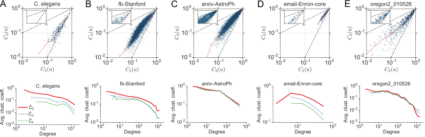
Figure 4: Top row: Joint distributions of ($C_{2}(u)$, $C_{3}(u)$) for (A) C. elegans (B) Facebook friendship, (C) arxiv co-authorship, (D) email, and (E) autonomous systems networks. Each blue dot represents a node, and the red curve tracks the average over logarithmic bins. The upper trend line is the bound in Eq. 14, and the lower trend line is expected Erdős-Rényi behavior from Proposition 3. Bottom row: Average higher-order clustering coefficients as a function of degree.

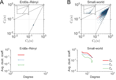
Figure 5: Analogous plots of Fig. 4 for synthetic (A) Erdős-Rényi and (B) small-world networks. Top row: Joint distributions of ($C_{2}(u)$, $C_{3}(u)$). Bottom row: Average higher-order clustering coefficients as a function of degree.

We emphasize that simple clique counts are not sufficient to obtain these results. For example, the discrepancy in the third-order average clustering of C. elegans and the MRCN null model is not simply due to the presence of 4-cliques. The original neural network has nearly twice as many 4-cliques (2,010) than the samples from the MRCN model (mean 1006.2, standard deviation 73.6), but the third-order clustering coefficient is larger in MRCN. The reason is that clustering coefficients normalize clique counts with respect to opportunities for closure.

Thus far, we have analyzed global and average higher-order clustering, which both summarize the clustering of the entire network. In the next section, we look at more localized properties, namely the distribution of higher-order local clustering coefficients and the higher-order average clustering coefficient as a function of node degree.

IV.3 Higher-order local clustering coefficients and degree dependencies

We now examine more localized clustering properties of our networks. Figure 4 (top) plots the joint distribution of $C_{2}(u)$ and $C_{3}(u)$ for the five networks analyzed in Table 2, and Fig. 5 (top) provides the analogous plots for the Erdős-Rényi and small-world networks. In these plots, the lower dashed trend line represents the expected Erdős-Rényi behavior, i.e., the expected clustering if the edges in the neighborhood of a node were configured randomly, as formalized in Proposition 3. The upper dashed trend line is the maximum possible value of $C_{3}(u)$ given $C_{2}(u)$, as given by Proposition 1.

For many nodes in C. elegans, local clustering is nearly random (Fig. 4, top), i.e., resembles the Erdős-Rényi joint distribution (Fig. 5, top). In other words, there are many nodes that lie on the lower trend line. This provides further evidence that C. elegans lacks higher-order clustering. In the arxiv co-authorship network, there are many nodes $u$ with a large value of $C_{2}(u)$ that have an even larger value of $C_{3}(u)$ near the upper bound of Eq. 14 (see the inset of Fig. 4, top). This implies that some nodes appear in both cliques and also as the center of star-like patterns, as in Fig. 2. On the other hand, only a handful of nodes in the Facebook friendships, Enron email, and Oregon autonomous systems networks are close to the upper bound (insets of Figs. 4,4, and 4, top).

Figures 4 and 5 (bottom) plot higher-order average clustering as a function of node degree in the real-world and synthetic networks. In the Erdős-Rényi, small-world, C. elegans, and Enron email networks, there is a distinct gap between the average higher-order clustering coefficients for nodes of all degrees. Thus, our previous finding that the average clustering coefficient $\bar{C}_{\ell}$ decreases with $\ell$ in these networks is independent of degree. In the Facebook friendship network, $C_{2}(u)$ is larger than $C_{3}(u)$ and $C_{4}(u)$ on average for nodes of all degrees, but $C_{3}(u)$ and $C_{4}(u)$ are roughly the same for nodes of all degrees, which means that 4-cliques and 5-cliques close at roughly the same rate, independent of degree, albeit at a smaller rate than traditional triadic closure (Fig. 4, bottom). In the co-authorship network, nodes $u$ have roughly the same $C_{\ell}(u)$ for $\ell=2$, $3$, $4$, which means that $\ell$-cliques close at about the same rate, independent of $\ell$ (Fig. 4, bottom). In the Oregon autonomous systems network, we see that, on average, $C_{4}(u)>C_{3}(u)>C_{2}(u)$ for nodes with large degree (Fig. 4, bottom). This explains how the global clustering coefficient increases with the order, but the average clustering does not, as observed in Table 1.

V Discussion

We have proposed higher-order clustering coefficients to study higher-order closure patterns in networks, which generalizes the widely used clustering coefficient that measures triadic closure. Our work compliments other recent developments on the importance of higher-order information in network navigation Rosvall et al. (2014); Scholtes (2017) and on temporal community structure Sekara et al. (2016); in contrast, we examine higher-order clique closure and only implicitly consider time as a motivation for closure.

Prior efforts in generalizing clustering coefficients have focused on shortest paths Fronczak et al. (2002), cycle formation Caldarelli et al. (2004), and triangle frequency in $k$-hop neighborhoods Andrade et al. (2006); Jiang and Claramunt (2004). Such approaches fail to capture closure patterns of cliques, suffer from challenging computational issues, and are difficult to theoretically analyze in random graph models more sophisticated than the Erdős-Rényi model. On the other hand, our higher-order clustering coefficients are simple but effective measurements that are analyzable and easily computable (we only rely clique enumeration, a well-studied algorithmic task). Furthermore, our methodology provides new insights into the clustering behavior of several real-world networks and random graph models, and our theoretical analysis provides intuition for the way in which higher-order clustering coefficients describe local clustering in graphs.

Finally, we focused on higher-order clustering coefficients as a global network measurement and as a node-level measurement, and in related work we also show that large higher-order clustering implies the existence of mesoscale clique-dense community structure Yin et al. (2017).