Hard-Core Bosons in flat band systems above the critical density

Abstract

We investigate the behaviour of hard-core bosons in one- and two-dimensional flat band systems, the chequerboard and the kagomé lattice and one-dimensional analogues thereof. The one dimensional systems have an exact local reflection symmetry which allows for exact results. We show that above the critical density an additional particle forms a pair with one of the other bosons and that the pair is localised. In the two-dimensional systems exact results are not available but variational results indicate a similar physical behaviour.

1 Introduction

Tight binding models are important to study the properties of correlated fermions or bosons. They describe interacting particles on a lattice. The most popular and important model of that kind is the Hubbard model [1, 2, 3], which was originally formulated for fermions and is known to describe many different phenomena, depending on the lattice structure and the interaction strength. The bosonic Hubbard model was introduced by Fisher et al. [4]. It is expected to show a similar rich phase diagram including a Mott insulator and a superfluid phase.

In the Hubbard model, the interaction of the particles is purely local and the hopping is often a nearest neighbour hopping. The hopping gives rise to bands. Strong correlations occur if the interaction strength is large compared to the band width.

Depending on the hopping matrix and on the structure of the lattice, one or more bands may be completely flat. A flat band system is of special interest if the physics of the system is mainly determined by particles in the flat band. For fermions this happens if at low temperatures the flat band is partially filled. For bosons the flat band must be at the bottom of the single particle spectrum to have a significant influence on the low temperature properties. In both cases, the interaction, even if it is small, dominates the behaviour of the system. A standard perturbational treatment of the interaction fails. Even an arbitrarily small interaction is larger than the band width and interesting correlation effects may occur. Flat band systems have been studied for more than 25 years, starting with magnetic properties of fermions in a flat band, see [5, 6, 7, 8, 9, 10] and the references therein. Starting in 2002, spin systems have been investigated in lattices with a flat band [11], see also [12] and the references therein. Approximately seven years ago flat band systems were first studied experimentally using optical lattices [13], see also [14]. Since in experiments it is possible to study bosons in flat bands, the theoretical interest in bosonic systems with flat bands started about the same time.

In a seminal paper, Huber and Altman [15] studied one- and a two-dimensional flat band systems with weakly interacting bosons. It turned out that it is important to understand the detailed structure of the single-particle eigenstates of the flat band. This is in contrast to fermions, where the detailed knowledge of the single-particle eigenstates of the flat band is less important, see e.g. the proofs in [16, 10, 17], which use only properties of the projector onto the flat band. In a flat band it is often possible to construct single-particle eigenstates that are localised on a finite set of lattice sites. This is also the case in the systems studied by Huber and Altman [15]. They showed that depending on the structure of the lattice and the structure of the local single-particle eigenstates, the systems may have different physical properties. Huber and Altman [15] investigated the formation of a Bose-Einstein condensate and a charge density wave. The saw-tooth chain they studied shows the formation of domain walls and a Luttinger liquid behaviour. Other authors showed that pairs of bosons are formed in flat band systems [18, 19, 20, 21] and other highly correlated phases [22].

It is clear that the flat band models must have more than one band, otherwise the physics of the system would be trivial. Therefore it is clear that the interesting phenomena observed in flat band systems occur because other bands are present as well, although they are energetically often less important. The reason is that the projector onto the flat band then has a certain structure which leads to effective interactions of longer range if one projects the interaction part of the Hamiltonian to the flat band. Huber and Altman [15] made use of this projection to construct an effective Hamiltonian with a more complicated structure which is responsible for the interesting physical properties they found. The main reason for these interactions is that the projector onto the flat band falls of algebraically in lattice space, the same is true for the Wannier states of the flat band. But it is clear that a projection onto the flat band is in essence a perturbative treatment of the system that is justified only for weak interactions.

In this paper we are interested in the opposite limit, strong interactions. We study hard-core bosons on a lattices with flat bands. The questions we want to answer are whether the phenomena predicted for weakly interacting systems occur for strong interactions as well and which new phenomena one can expect. Models with hard-core bosons can be mapped to spin-1/2 systems, since only two states per lattice site are allowed. In fact, the model we discuss in the present paper is equivalent to such a spin system in a strong magnetic field. The localised states in the flat band directly translate to localised magnons and multi-magnon states which have been investigated intensively, see the review of Derzhko et al. [12] and the references therein. The upper critical density appears in those systems as well, see e.g. [23, 24]. For a class of flat band systems, line graphs of plane graphs, Motruk and Mielke [25] showed rigorously how all multi-particle eigenstates at and below that critical density can be constructed. In [24], the linear independence of a subclass of the complete set on some of those lattices was shown in the context of spin systems. Since the bosons sit in non-overlapping single particle states, the interaction strength plays no essential role, all the results apply to hard core bosons as well. The kagomé lattice and some other lattices mentioned above fall into this class. The question therefore is, what happens at densities above the critical density. The pair formation mentioned above occurs above the critical density and was found in some one-dimensional systems with stronger interactions [18, 19, 20, 21].

The paper is organised as follows. The next section contains some definitions. We fix the notation and introduce some notions from graph theory needed. We also explain details about the critical density, following [25]. In section 3 we treat a special class of one-dimensional systems, with the chequerboard chain and the kagomé chain as examples. Both are line graphs. Both have a local reflection symmetry which allows us to obtain exact results. We show that pairs are formed and that the pairs are localised. In section 4 the two-dimensional kagomé lattice and the chequerboard lattice are discussed. Here as well we find strong indications for pair formation. The results are based on the numerical diagonalisation of small systems and on a variational ansatz. Finally we summarise and discuss our results.

2 Definitions

The Hubbard model is usually defined on a lattice or more general on a set of vertices $V$. In this paper we consider a bosonic Hubbard model with bosons which have no internal degree of freedom. The Hamiltonian can be written in the form

$$H=\sum_{x,y\in V}t_{xy}b_{x}^{\dagger}b_{y}+\sum_{x\in V}U_{x}b_{x}^{\dagger}b_{x}^{\dagger}b_{x}b_{x}$$ (1)

where $T=(t_{xy})_{x,y\in V}$ is the hopping matrix which describes the hopping of the bosons in a tight binding picture and $U_{x}>0$ are the local, repulsive interactions. We use the usual notation with creation operators $b_{x}^{\dagger}$ and annihilation operators $b_{x}$ with the usual bosonic commutation relations $[b_{x},b_{y}]=[b_{x}^{\dagger},b_{y}^{\dagger}]=0$ and $[b_{x},b_{y}^{\dagger}]=\delta_{xy}$.

We will treat this Hamiltonian on a special class of lattices, line graphs of plane graphs, which we define in the next subsection. The important property of these lattices is that the lowest eigenvalue of the hopping matrix is highly degenerate. In the case of translationally invariant lattices, the lowest band is flat. But this is not the only important property of these systems.

Further, we are interested in the limit of hard-core bosons, i.e. we assume that the limit $U_{x}\rightarrow\infty$ is taken. This means that on each vertex we may have at most one particle. We introduce the projector $P_{\leq 1}$ which projects onto the subspace of the multi particle Hilbert space which fulfils that property. The Hamiltonian can then be written as

$$H=P_{\leq 1}\sum_{x,y\in V}t_{xy}b_{x}^{\dagger}b_{y}P_{\leq 1}$$ (2)

2.1 Line graphs of plane graphs

We consider the Hubbard Hamiltonian on a graph $G=(V(G),E(G))$. $V(G)$ is the set of vertices, $E(G)$ the set of edges of $G$. An edge connects exactly two vertices. We consider only undirected graphs, therefore an edge $e\in E(G)$ is a subset of $V(G)$ with exactly two elements. The hopping matrix elements in (1) are $t_{xy}=1$ if $\{x,y\}\in E(G)$, 0 otherwise.

In a graphical representation, the vertices are drawn as dots, connected with lines, the edges. A graph that can be drawn in a plane without crossings of edges is called a plane graph. For details we refer to [26]. The edges of the plane graph divide the plane into many finite and one infinite part, which are called faces. We denote the set of bounded faces by $F(G)$. Single bounded faces are denoted by $\lambda\in F(G)$. We denote by $\lambda$ the face and also the set of edges of the boundary of $\lambda$. The boundary of a face is an elementary cycle of $G$.

In [25] it was shown rigorously that for a certain class of lattices, line graphs of bipartite plane graphs, there exists a critical particle number $N_{c}$. For a system with $N\leq N_{c}$ hard-core bosons, it is possible to describe all ground states completely. In this section we review some of the definitions and results of [25] which we need in the following.

Let $G=(V(G),E(G))$ be a connected bipartite plane graph. Bipartite means that $V(G)=V_{1}\cup V_{2}$ with $V_{1}\cap V_{2}=\emptyset$ and $|e\cap V_{i}|=1$ for all $e\in E(G)$ and $i=1,2$. If two vertices are connected, they are not on the same subset.

According to Eulers theorem, a plane graph has $|F(G)|=|E(G)|-|V(G)|+1$ bounded faces.

To a graph $G$ one associates various matrices. The most important is the adjacency matrix $A(G)=(a_{xy})_{x,y\in V(G)}$ where $a_{xy}=1$ if $\{x,y\}\in E(G)$, $a_{xy}=0$ otherwise. A second important matrix is the vertex-edge incidence matrix $B(G)=(b_{xe})_{x\in V(G),e\in E(G)}$ where $b_{xe}=1$ if $x\in e$, $b_{xe}=0$ otherwise.

The line graph $L(G)=(V(L(G),E(L(G)))$ of $G$ is constructed as follows: $V(L(G))=E(G)$, $E(L(G))=\{\{e,e^{\prime}\}:\,e,e^{\prime}\in E(G)\,\mbox{and}\,|e\cap e^{\prime}|=1\}$. It is easy to see that $A(L(G))=B(G)^{\dagger}B(G)-2$. As a consequence, the lowest eigenvalue of $A(L(G))$ is $-2$ and it is $|F(G)|$ fold degenerate. Let us remark that if $G$ is a tree, $|F(G)|=0$ and there is no state with energy -2. As shown in [27], a basis of the eigenstates for the eigenvalue $-2$ can be constructed using the boundaries of the bounded faces $\lambda\in F(G)$ of $G$. Each bounded face is bounded by an elementary cycle of even length, because the graph $G$ is bipartite. Each face can be oriented clockwise. Each edge of $G$ can be oriented to point from one of the two subsets of $V(G)$ to the other. Now let $v_{\lambda}=(v_{\lambda e})_{e\in E(G)}$ be defined for a face $\lambda$ of $G$ as follows: $v_{\lambda e}=1$ if $e\in\lambda$ and $e$ and $\lambda$ have the same orientation, $v_{\lambda e}=-1$ if $e\in\lambda$ and $e$ and $\lambda$ have the opposite orientation, $v_{\lambda e}=0$ otherwise. It is easy to see that $A(L(G))v_{\lambda}=-2v_{\lambda}$. Since there are $|F(G)|$ bounded faces, which form a set of linear independent $v_{\lambda}$, these states form a basis of the eigenstates for the eigenvalue $-2$. For later use we define creation operators $b_{\lambda}^{\dagger}=\frac{1}{\sqrt{|\lambda|}}\sum_{e\in\lambda}v_{\lambda e}b_{e}^{\dagger}$ and the corresponding annihilation operators.

Important examples of line graphs in two dimensions are the kagomé lattice, the line graph of the honeycomb lattice, and the chequerboard lattice, the line graph of the square lattice. For further details and examples we refer to [6, 27].

2.2 Multi-particle states

Consider now the Hamiltonian (2) with the hopping matrix $A(L(G))$ on the graph $L(G)$ with $N$ hard-core bosons. Let $C\subset F(G)$ be a subset of non edge-sharing faces. It is then clear that the state $\prod_{\lambda\in C}b_{\lambda}^{\dagger}|0\rangle$ is a ground state of $H$ with energy $-2|C|$. Clearly, there is some maximal particle number $N_{c}$ for which that construction is possible. Further, the states constructed in this way are not complete. In [25] it was shown how all ground states with $N\leq N_{c}$ can be constructed. Further, $N_{c}$ is related to the colouring of the faces of $G$. Since for $N=N_{c}$ all occupied faces have no edge in common, they can be coloured with one colour. On the other hand, if there was a colouring of the faces of $G$ where more than $N_{c}$ faces are coloured with the same colour, we could choose this colour and put a particle on each face. But then there would be a state with energy $-2N$ and since $N\leq N_{c}$ we would have a contradiction. Therefore, $N_{c}$ is the number of elements in the largest subset of faces of $G$ that can be coloured with the same colour. The question we wish to address in this paper is what happens if one adds a small number of additional particles to this system.

Whereas for $N\leq N_{c}$, a mathematically rigorous description of the ground states is possible, there are no rigorous results for $N>N_{c}$ so far. To gain some insight here, we use different approaches, a variational ansatz and numerical diagonalisation of small systems. For both cases, we need to restrict ourselves to special lattices. We consider one- and two-dimensional examples derived from the chequerboard and the kagomé lattice.

3 One dimensional systems

In this section we restrict ourselves to planar bipartite graphs with the additional property that in a colouring of faces, all elements of $F(G)$ can be coloured by the same colour. Any two faces have at most one vertex in common. This class of one-dimensional systems are chains of even cycles or single edges having a single vertex in common. Since the graphs in the class are chains of faces, we enumerate the faces by numbers $1$ to $|F(G)|$ such that the neighbouring faces of the face $\lambda$ are $\lambda\pm 1$.

For each element in this class, we have $N_{c}=|F(G)|$. This simplifies the proof of completeness of multi-particle states for $N\leq N_{c}$ a lot and makes calculations for $N>N_{c}$ easier. For $N=N_{c}$ there is one single ground state $\prod_{\lambda\in F(G)}b_{\lambda}^{\dagger}|0\rangle$.

The Hamiltonian of hard core bosons on the line graph $L(G)$ can be written in the form

$$H=H^{\prime}+H^{\prime\prime}=\sum_{\lambda\in F(G)}H_{\lambda}+\sum_{\lambda\in F(G)\setminus\{|F(G)|\}}H_{\lambda,\lambda+1}$$ (3)

where $H_{\lambda}$ contains hoppings on the edges of the face $\lambda$ and $H_{\lambda,\lambda+1}$ contains the hoppings between the neighbouring faces $\lambda$ and $\lambda+1$. To fix our notation, we write

$$H_{\lambda}=P_{\leq 1}\sum_{i\in\lambda}b_{\lambda,i}^{\dagger}b_{\lambda,i+1}P_{\leq 1}+\mathrm{h.c.}$$ (4)

where the edges of $\lambda$ are numbered in a cyclic manner by an integer $i$ modulo $|\lambda|$. As introduced above, $P_{\leq 1}$ is the projector onto the subspace with at most one boson on each vertex of $L(G)$, reflecting the hard core interaction.

Two neighboured faces $\lambda$ and $\lambda+1$ have at most one vertex in common. If they have no vertex in common, there is exactly one vertex in $\lambda$ and one vertex in $\lambda+1$ which are connected by an edge or a chain of edges. Let $i,i+1$ be the two edges of $\lambda$ connected to the vertex that connects $\lambda$ to $\lambda+1$. By construction, since $L(G)$ is a line graph, $H_{\lambda,\lambda+1}$ is symmetric against an exchange of the two edges $i$ and $i+1$. An operator that exchanges the two edges is a reflection operator of the face $\lambda$. We denote this operator by $S_{\lambda}$. We restrict ourselves to graphs $G$ where $H$ commutes with all local reflections $S_{\lambda}$, $\lambda\in F(G)$.

Since all $S_{\lambda}$ commute among themselves and with $H$, all eigenstates of $H$ are eigenstates of $S_{\lambda}$ as well. Each eigenstate of $H$ can therefore be characterised by a signature $(s_{\lambda})_{\lambda\in F}$, where $s_{\lambda}$ takes the values $\pm 1$. For the above defined operator $b_{\lambda}^{\dagger}=\frac{1}{\sqrt{|\lambda|}}\sum_{e\in\lambda}v_{\lambda e}b_{e}^{\dagger}$ , the application of the reflection operator yields $S_{\lambda}b_{\lambda}^{\dagger}S_{\lambda}=-b_{\lambda}^{\dagger}$. Therefore, the unique ground states for $N=N_{c}$, $\prod_{\lambda\in F(G)}b_{\lambda}^{\dagger}|0\rangle$, has eigenvalues $-1$ for all $S_{\lambda}$.

Let us now add a particle to the system, so that $N=N_{c}+1$. Let us first consider only $H^{\prime}$. We obtain ground states for $H^{\prime}$ by putting the additional particle on one of the faces $\lambda$. The resulting ground state has thus two particles on one face $\lambda$ and $s_{\lambda}=1$ for that face, $s_{\lambda}=-1$ for all other faces. If the elementary cycles $\lambda$ have different length, it is energetically favourable to put the two particles on the longest cycle. Let $\ell=\max_{\lambda\in F(G)}|\lambda|$ be the length of the longest elementary cycle. If there are several cycles of the same length, the ground state of $\sum_{\lambda}H_{\lambda}$ will be degenerate. The most interesting case is clearly the one where all cycles have the same length, in that case the ground state $\sum_{\lambda}H_{\lambda}$ with $N=N_{c}$ particles will be $N_{c}$-fold degenerate.The question is now, what happens if we add the hopping between the faces, $\sum_{\lambda}H_{\lambda,\lambda+1}$. In that case, the pair of particles sitting on one of the faces can gain some energy by spreading to the neighboured faces, the ground state energy gets lower. But, since all $H_{\lambda,\lambda+1}$ obey the same symmetry, we may expect to get still a ground state with a signature, where all $s_{\lambda}$ are $-1$ except one, which has $+1$. This idea has an immediate problem: Suppose that there are many edges between two neighboured faces $\lambda$ and $\lambda+1$. Then, spreading the additional particle on these edges, the particle can gain an energy close to $-2$, which is the energy on an infinitely long chain. Therefore we restrict ourselves to chains with at most a single edge between two faces. To proceed, we treat two examples, the chequerboard chain and a kagomé chain. The chequerboad chain is the line graph of a chain of vertex sharing squares. The kagomé chain is the line graph of a chain of disjoint hexagons connected by additional edges, one between each pair of neighboured hexagons see Fig. 1, which also shows its construction as a line graph.

Figure 1: A part of the kagomé chain, the line graph of a chain of hexagons connected by additional edges.

Let us mention that other kagomé chains have been proposed and treated before, esp. in the context of frustrated spin systems, see [28, 29, 11]. None of those falls into the class of models discussed here. These one-dimensional lattices are line graphs; the kagomé like chain of [28] is the line graph of a chain of edge sharing squares, the one in [29] a chain of edge sharing hexagons, both are discussed in [11]. For these models, $N_{c}=|F(G)|/2$, not $N_{c}=|F(G)|$ as in the class of models we are treating here.

3.1 The chequerboard chain

Let $G$ be a chain of squares which have one vertex in common. The line graph of $G$ is the chequerboard chain. A part of the chequerboard chain $L(G)$ is depicted in Fig. 2. Each face contains four edges of $G$ numbered as depicted in 2. With this notation the Hamiltonian can be written as in (3) with

$$H_{\lambda,\lambda+1}=P_{\leq 1}(b_{\lambda,1}^{\dagger}+b_{\lambda,2}^{\dagger})(b_{\lambda+1,0}+b_{\lambda+1,3})P_{\leq 1}+\mathrm{h.c.}$$ (5)

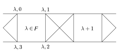
Figure 2: A part of the chequerboard chain, the line graph of a chain of corner sharing squares.

The operator that performs the local reflection has the explicit form

$$S_{\lambda}=\exp(\frac{i\pi}{2}((b_{\lambda,1}^{\dagger}-b_{\lambda,2}^{\dagger})(b_{\lambda,1}-b_{\lambda,2})+(b_{\lambda,0}^{\dagger}-b_{\lambda,3}^{\dagger})(b_{\lambda,0}-b_{\lambda,3}))).$$ (6)

To verify that, notice first that since $b_{\lambda,1}^{\dagger}+b_{\lambda,2}^{\dagger}$ commutes with $b_{\lambda,1}-b_{\lambda,2}$, it commutes also with $S_{\lambda}$. Further, $S_{\lambda}^{\dagger}(b_{\lambda,1}^{\dagger}-b_{\lambda,2}^{\dagger})S_{\lambda}=\exp(i\pi)(b_{\lambda,1}^{\dagger}-b_{\lambda,2}^{\dagger})=-(b_{\lambda,1}^{\dagger}-b_{\lambda,2}^{\dagger}).$ Therefore, $S_{\lambda}^{\dagger}b_{\lambda,1}^{\dagger}S_{\lambda}=b_{\lambda,2}^{\dagger}$, and similarly for $b_{\lambda,0}^{\dagger}$ and $b_{\lambda,3}^{\dagger}$.

We start with open boundary conditions and let $N=N_{c}+1$, i.e. we put one additional particle in the system. The results of a numerical diagonalisation of small systems is shown in table 1. The second column contains $\Delta E=E+2N_{c}$. For longer chains the lowest eigenvalue stays at -1.0165. A trivial upper bound for $\Delta E$ is $\Delta E<-2\sqrt{2}+2=-0.8284$. Since $-2\sqrt{2}$ is the ground state energy of two hard-core bosons on a square, the ground states of $H^{\prime}$ have exactly $\Delta E=-2\sqrt{2}+2$. Since the ground state of a doubly occupied square has $s_{\lambda}=1$, the ground state of $H^{\prime}$ is exactly $|F(G)|$-fold degenerate. Adding $H^{\prime\prime}$ to $H^{\prime}$ lowers the energy of the eigenstates. Note that for the lattices in table 1 there are exactly $N_{c}$ states with $\Delta E<-2\sqrt{2}+2$.

Looking at the states shown in table 1 shows that they have a strong overlap with states where one face is occupied by two hard-core bosons and all the other faces are occupied by one particle. Adding $H^{\prime\prime}$ to $H^{\prime}$ has the effect that the additional particle spreads slightly on the other faces, thereby lowering the energy of the pair. But it does not change the symmetry properties of the ground state, the signature $(s_{\lambda})_{\lambda\in F(G)}$. The reason is that the ground states of $H^{\prime}$ have a non-zero overlapp with the low energy states of $H$, since $H^{\prime\prime}$ respects the symmetry and higher energy states of $H^{\prime}$ are not lowered enough to become new ground states of $H$. The signatures of the states are $-1$ on all faces except one, which has $+1$. This face is the doubly occupied face. Only at the boundary the lowering is somewhat less, therefore we obtain two states with an energy -0.920 for the lattices in table 1. This is due to the fact, that the two-particle ground state on a single square has signature $+1$, so there must be a state with an energy lower than the trivial one in each of these $N_{c}$ subspaces and by table 1, only $N_{c}$ such states exist.

lattice	all eigenvalues ($\Delta E$) below$-2\sqrt{2}+2$
	-0.920; -0.920
	-1.0162 -0.920; -0.920
	-1.0163; -1.0163 -0.920; -0.920
	-1.0165 -1.0164; -1.0164 -0.920; -0.920
	-1.0165; -1.0165 -1.0164; -1.0164 -0.920; -0.920

Table 1: Eigenvalues of finite open parts of the chequerboard chain with $N_{c}+1$ bosons. The eigenvalues are shown relative to the ground state energy of the system with $N_{c}$ bosons, $\Delta E=E+2N_{c}$.

From the ground state one can calculate the occupation numbers on the faces. The number of particles on the face $\lambda$ is $n_{\lambda}=\sum_{i\in\lambda}n_{\lambda,i}=\sum_{i\in\lambda}b_{\lambda,i}^{\dagger}b_{\lambda,i}$. For the ground state of the lattice with five faces we obtain $\langle n_{2}\rangle=1.91$, $\langle n_{1}\rangle=\langle n_{3}\rangle=1.04$, $\langle n_{0}\rangle=\langle n_{4}\rangle=1.000004$. For longer chains, the density on more distant squares is 1 within the numerical accuracy. This shows that the additional boson forms a pair on one face and that the pair is strongly localised. It is spread a bit on the nearest neighboured faces and to a very low portion to the next neighboured faces.

Let us now assume that we have periodic boundary conditions and an arbitrary $N$. Let us assume that we have an eigenstate of $H$ with a signature $(s_{\lambda})_{\lambda\in F(G)}$. Then, because of the translational symmetry of the Hamiltonian, the state that is translated by 1 face is as well an eigenstate, it has the signature $(s_{\lambda}^{\prime})$ with $s_{\lambda}^{\prime}=s_{\lambda+1}$. As a consequence, we get degeneracies in the spectrum of $H$. The degeneracies are multiples of divisors of $|F(G)|$.

For a chain with periodic boundary conditions and $N=N_{c}+1$ we obtain degenerate ground states at energy -1.0165. As for the open chain, the signatures of the states are $-1$ on all faces except one, the doubly occupied face, which has $+1$. Due to the translational symmetry, there are exactly $|F(G)|$ degenerate states, which are found in the numerical diagonalisation of systems with small $|F(G)|$. The reasoning is the same as above, the ground states of $H$ have a finite overlap with the ground states of $H^{\prime}$ and therefore must have the same symmetry properties, which directly yields the $|F(G)|$-fold degeneracy.

This analysis is not rigorous in a mathematical sense because it relies on numerical diagonalisations of small systems. But since the symmetry is exact, the localisation of the eigenstates is very strong, and the eigenvalues do not change for longer chains, we believe to have a very strong argument that the analysis holds true for arbitrary long chains. The physical picture for additional hard-core bosons added to the chequerboard chain is that we obtain an effective flat band for these particles, that for $n\ll|F(G)|$ additional particles the ground state energy is $E=-2|F(G)|-1.0165n$ and that the additional particles form localised pairs with the particles already present. We checked that numerically for $n=2$. The two pairs try to separate. On sufficiently long chains, the ground state energy is indeed $E=-2|F(G)|-2\times 1.0165$. For shorter chains, the pairs start to overlap and the energy rises. This is physically intuitive: due to the spread of the pair state to neighboured faces, the pairs will try to keep some distance from each other, having an effective repulsive short-range interaction.

The derivation of this physical picture relies on the local reflection symmetry combined with the translation symmetry of the chequerboard chain. The question is whether a similar picture is true for other one-dimensional lattices without a local reflection symmetry or even for two dimensional systems.

3.2 Kagomé chain

The kagomé chains we treat here is the line graph $L(G)$ of a graph $G$ that is a chain of hexagons connected by a single edge between neighboured hexagons, see Fig. 1. This kagomé chain contains therefore interstitial sites, which are important for weakly interacting bosons on the two-dimensional kagomé lattice [15]. For this chain, we can proceed as for the chequerboard chain, and the results are similar. We therefore do not repeat each argument above, but only state the results. For chains with periodic boundary conditions, we obtain $|F(G)|$-fold degenerate ground states with an energy $\Delta E=-1.6046$. The states are localised. The occupation numbers are 1.80 for the central hexagon, 0.086 for the neighboured interstitial sites, and 1.014 for the neighboured hexagons. Within the numerical accuracy the density on more distant hexagons is 1. For longer open chains, the ground states also have the same energy starting with a chain of three hexagons. This and the fact that even for three hexagons $\Delta E$ has the energy of the chain with periodic boundary conditions indicate that the localisation of the pair is even stronger than for the chequerboard chain. The physical reason may be that it is energetically easier to put two hard core bosons on a hexagon than on a square. For the open chains, we find two states with a somewhat higher energy $\Delta E=-1.518$ corresponding to states localised on the two outer hexagons.

As for the chequerboard chain, we get an effective flat band for the additional particle. Due to the strong localisation, adding $n\ll|F(G)|$ additional particles the ground state energy is $E=-2|F(G)|-1.6046n$ and that the additional particles form localised pairs with the particles already present.

As for the chequerboard chain, the results rely on numerical diagonalisations of small systems. But for the same reasons as above, we expect them to be true for arbitrary long chains. In both cases, we get an entirely flat band for the additional particle in a chain with periodic boundary conditions. The additional particle forms a localised pair. For open boundary conditions the band is almost flat, there are edge states with a somewhat higher energy.

4 Two-dimensional systems

In this section, we treat two-dimensional systems of which the one-dimensional systems of the previous section are sublattices: The kagomé lattice and the chequerboard lattice. These two-dimensional systems have no local reflection symmetry. We base our analysis on variational states and numerical diagonalisations of small systems.

We start our analysis with the kagomé lattice because it is itself a plane graph and because it has interstitial sites. Interstitial sites give some additional space for additional particles above the critical density. Therefore, some other states, which do not consist of pairs, may be more favourable. Further, the question of pair formation on the chequerboard lattice has been discussed already in [21] and therefore a lengthy treatment is not necessary here.

4.1 The kagomé lattice

Let $F_{1}$ be one of the three subsets of non edge-sharing faces of $F(G)$ where $G$ is now the honeycomb lattice and $L(G)$ is the kagomé lattice. We assume that we have open boundaries and that $F_{1}$ is the largest of the three subsets of non edge-sharing faces. Let $F_{1}^{\dagger}=\prod_{\lambda\in F_{1}}b_{\lambda}^{\dagger}$. The state $|F_{1}\rangle=F_{1}^{\dagger}|0\rangle$ is a ground state of the system for $|F_{1}|$ particles. If $|F_{1}|=|F(G)|/3$, there are two more ground state with the same particle number but formed on one of the other two subsets of non edge-sharing faces.

The difference between the kagomé lattice and the chequerboard lattice, see below, is that the former contains interstitial sites, sites which are not occupied in $|F_{1}\rangle$. Huber and Altman treated the bosonic Hubbard model on the kagomé lattice for weak interaction and found that the additional particle gets delocalised, mainly because of the interstitial sites.

To investigate the role of the interstitial sites and a possible delocalisation, we construct a variational state

$$|X_{\leq 1}\rangle=P_{\leq 1}\psi^{\dagger}|F_{1}\rangle$$ (7)

$$\psi^{\dagger}=\sum_{e\in E(G)}\psi_{e}b_{e}^{\dagger}$$ (8)

Denote $|\psi\rangle=\psi^{\dagger}|0\rangle$ the corresponding single particle state. Then we obtain

$$\frac{\langle X_{\leq 1}|H|X_{\leq 1}\rangle}{\langle X_{\leq 1}|X_{\leq 1}\rangle} = \frac{\langle\psi|F_{1}P_{\leq 1}HP_{\leq 1}F_{1}^{\dagger}|\psi\rangle}{\langle\psi|F_{1}P_{\leq 1}F_{1}^{\dagger}|\psi\rangle}$$ (9)

Introducing the matrices $M=(m_{ee^{\prime}})_{e,e^{\prime}\in E(G)}$ and $C=(c_{ee^{\prime}})_{e,e^{\prime}\in E(G)}$ where

$$m_{ee^{\prime}}=\langle 0|b_{e^{\prime}}F_{1}P_{\leq 1}(H+2|F_{1}|)P_{\leq 1}F_{1}^{\dagger}b_{e}^{\dagger}|0\rangle$$ (10)

and

$$c_{ee^{\prime}}=\langle 0|b_{e^{\prime}}F_{1}P_{\leq 1}F_{1}^{\dagger}b_{e}^{\dagger}|0\rangle$$ (11)

we can write the variational energy as

$$\frac{\langle X_{\leq 1}|H|X_{\leq 1}\rangle}{\langle X_{\leq 1}|X_{\leq 1}\rangle} = -2|F_{1}|+\frac{\langle\psi|M|\psi\rangle}{\langle\psi|C|\psi\rangle}$$ (12)

The second term in this equation is $\Delta E$, the energy of the additional particle. $M$ and $C$ can be calculated to be

$$M =H-\frac{1}{3}(HP_{F(G)}+P_{F(G)}H)+\frac{2}{3}P_{F}-2P_{F_{1}}$$ (13)

$$C =1-\frac{1}{3}P_{F(G)}+P_{F_{1}}$$ (14)

where $(P_{F(G)})_{e,e^{\prime}}=\delta_{e\in F(G)}\delta_{ee^{\prime}}$ is the projector on $F(G)$ and $(P_{F_{1}})_{ee^{\prime}}=\frac{1}{6}\sum_{\lambda\in F}\nu_{\lambda e}\nu_{\lambda e^{\prime}}$ is the projector on the one-particle states that $F_{1}$ is build of. Since eigenvalues for projectors are 0 or 1, $C$ is positive definite and therefore it is possible to introduce a new scalar product $\{\phi|\psi\}=\langle\phi|C|\psi\rangle$. Using this notation one obtains $\Delta E=\frac{\{\psi|C^{-1}M|\psi\}}{\{\psi|\psi\}}$. The matrix $C^{-1}M$ can be calculated by noting that $C^{-1}=1+\frac{1}{2}P_{F(G)}-\frac{9}{10}P_{F_{1}}$. Due to the translational invariance of the lattice and the state $|F_{1}\rangle$ we can apply a Fourier transform. For the kagomé lattice, the resulting matrix which has to be diagonalised is a $9\times 9$-matrix. We obtain $9$ energy bands for the additional particle using the variational ansatz.

Figure 3: Lowest three energy bands of an additional particle added to the ground state $|F_{1}\rangle$ within the variational ansatz (9).

In Fig. 3 we show the lowest three energy bands. We obtain two dispersive bands and one flat band, the latter is not at the bottom of the spectrum. The lowest energy is $\Delta E=-1.52$.

In [21] it was shown that putting an additional particle onto an already occupied face $\lambda$, one obtains the energy $\mbox{$\Delta$E=}2-2\sqrt{3}=-1.46$. The variational state constructed above has a lower energy which indicates that the particle gains some energy due to the delocalisation. On the other hand, Pudleiner et al. [21] also considered the subunit shown in Fig. 4. Adding a particle to that subunit one obtains four states with an energy below -1.46. Three of them are almost degenerate at energies $\Delta E=-1.55$ and $\Delta E=-1.56$ corresponding to linear combinations of the doubly occupied faces, the fourth has the energy $\Delta E=-1.66$. In this state, the interstitial sites are occupied as well. These energies are upper bounds to the true energy of the additional particle on the kagomé lattice. Decorating the subunit with 12 additional sites, see Fig. (4), one obtains somewhat lower energies, $\Delta E=-1.69$ and $\Delta E=-1.75$. These are no upper bounds since the additional sites would touch occupied faces. The energies are lower, so the additional particle gets further delocalised onto the additional sites, but the amplitudes on these sites are low, 0.008 and 0.003, showing that the trend to delocalise the particle further is not high. All these energies are lower than the lowest energy of the variational ansatz (9), which shows that the energy gain due to delocalisation is smaller than the energy gain one obtains if the particle is in a localised state and arranges itself in an optimal way with its neighbours.

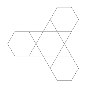
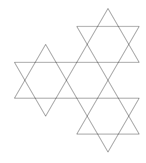
Figure 4: non-decorated and decorated subunits of the kagomé lattice.

4.2 The chequerboard lattice

Localised pairs on the chequerboard lattice have been proposed in [21]. Diagonalising a subunit of the chequerboard lattice with five squares and five bosons (one more than $|F(G)|$) they found four almost degenerate states, the lowest having $E=-2|F(G)|-1.081$, the additional particle has an energy $-1.081$. This energy is a variational upper bound of the true ground state energy in a system with large $|F(G)|$. The four states have a large overlap with the states where a pair of bosons is localised on one square. The energy is lowered and the degeneracy is lifted, although only weakly, because the pair spreads a bit, as for the chain. Note that the energy is significantly lower than for the chain with five squares, indicating that the delocalisation is larger here.

The variational calculation is possible on the kagomé lattice, because there the matrix $M$ has a relatively simple form. The reason is that a particle hopping from a site on a face $\lambda$ to some site not in $\lambda$ hops to an interstitial site. A single hopping never transfers the particle to a neighboured face. On the chequerboard lattice this is not true. Therefore, the same variational calculation on the chequerboard lattice yields an additional term in (13). The calculation is still possible but does not yield additional insight.

5 Summary and Outlook

The aim of this paper is to investigate hard-core bosons in a flat band system. We first looked at two one-dimensional systems, a chequerboard chain and a kagomé chain. The chequerboard chain is the line graph of a chain of corner sharing squares. The kagomé chain is a line graph of a chain of hexagons connected by additional edges. As line graphs, both have a lowest flat band. Further, both have a local reflection symmetry. Applying the reflection of a single square or hexagon, an eigenstate of the Hamiltonian is either symmetric or antisymmetric. At the critical density, each square or hexagon is occupied by a single particle and the ground state is antisymmetric with respect to all local reflections. Adding a single particle to the system, the ground state of the chain becomes symmetric for one local reflection and remains antisymmetric for all others. In the case of periodic boundary conditions, we obtain a degeneracy given by the number of squares or hexagons. For open boundary conditions, most of the states are almost degenerate except for those where the state is symmetric with respect to reflection of the first or last square or hexagon. At the boundary, the additional particle has a slightly higher energy.

In the ground states with one additional particle, this particle forms a pair with another particle. The lowest state with one particle on the square or hexagon is antisymmetric, with two particles it is symmetric. This explains the symmetry of the states and the degeneracy. Looking closer at the states we find that the pair which is formed is localised. Effectively, we obtain a flat band for the additional particle. The localisation is not perfect in the sense that the pair is strictly localised on a single square or hexagon, but the expectation value of occupation number falls of very rapidly. For the chains, already at a distance of three faces, the excess density is 0 within the numerical accuracy. This means that even at a finite but low density above the critical density we expect the ground state to be degenerate and to be formed of well separated localised pairs and single particles in between. The numerical results for two additional particle on finite chains support that view.

In two dimensions, the chequerboard and kagomé lattice are line graphs as well with a lowest flat band. But for the two-dimensional systems, there is no exact local symmetry. Therefore, it is not possible to obtain exact results as for the one-dimensional analogues. Here, we use two variational ansatzes, one with possibly extended states and one with localised states on small compounds. The best variational states for the two systems again show localised pairs, although the localisation is less perfect than in the one-dimensional case. But we have a strong indication that here as well the additional particle forms a localised pair and that one obtains an effectively flat band for the additional particles at low densities.

Since pair formation was observed in other one- and two-dimensional bosonic flat band systems as well [18, 19, 20, 21], this seems to be a universal feature of these systems. But whether or not this is really the case remains open. Whereas for fermions in a flat band a full characterisation of the ground states is possible at and below half filling of the flat band, this is not the case for bosons. For fermions, a detailed knowledge of the single-particle eigenstates is not necessary, often some properties of the projector are sufficient to obtain the desired result. In contrast, for bosons, the knowledge of the single particle states and, in the case of the two one-dimensional systems discussed here, their symmetry is important to understand the underlying physics of the system. This makes the treatment of interacting bosons in a flat band much more challenging.

The kagomé lattice has been realised as an optical lattice [14, 13] and experiments are possible which may allow to investigate pair formation. For the chequerboard lattice an experimental realisation may be difficult or even impossible. But the flat band states of the chequerboard lattice are similar to those in the Lieb lattice [6], there is a one-to-one mapping of the single particle states in the flat bands of these two lattices. Adding additional on site energies to the Lieb lattice or next nearest neighbour hoppings, it is even possible to shift the flat band to the bottom of the spectrum. The Lieb lattice has been realised as an optical lattice as well [30]. Therefore it may be possible to investigate pair formation in the Lieb lattice. To our knowledge, hard core bosons in a Lieb lattice have not been studied so far.

Author contribution statement: Both authors contributed equally to the paper.

References

- [1] J Hubbard. Proc. Roy. Soz. A 276, 238 (1963).
- [2] J Kanamori. Prog. Theor. Phys. 30, 275 (1963).
- [3] M. C. Gutzwiller. Phys. Rev. Lett. 10, 159 (1963).
- [4] M.P.A. Fisher, P.B. Weichman, G. Grinstein, D.S. Fisher. Phys. Rev. B 40, 546 (1989).
- [5] E H Lieb. Phys. Rev. Lett.62, 1201 (1989).
- [6] A Mielke. J. Phys. A: Math. Gen. 24, 3311 (1991).
- [7] H Tasaki. Phys. Rev. Lett. 69, 1608 (1992).
- [8] A. Mielke, H. Tasaki. Commun. Math. Phys. 158, 341 (1993).
- [9] H Tasaki. cond-mat/9712219 (1997).
- [10] A Mielke. J. Phys. A, Math. Gen., 32, 8411 (1999).
- [11] J. Schulenburg, A. Honecker, J. Schnack, J. Richter, and H.-J. Schmidt. Phys. Rev. Lett. 88, 167207 (2002).
- [12] O. Derzhko, J. Richter, A. Honecker, and H.-J- Schmidt. Low Temp. Phys. 33, 745 (2007).
- [13] G.-B. Jo, J Guzman, C K Thomas, P Hosur, A Vishwanath, D M Stamper-Kurn. Phys. Rev. Lett. 108, 045305 (2012).
- [14] J Ruostekoski. Phys. Rev. Lett. 103, 080406 (2009).
- [15] S D Huber, E Altman. Phys. Rev. B 82, 184502 (2010).
- [16] A. Mielke. Physical Review Letters 82, 4312 (1999).
- [17] A. Mielke. Eur. Phys. J. B 85, 1 (2012).
- [18] S. Takayoshi, H. Katsura, N. Watanabe, H. Aoki. Phys. Rev. A 88, 063613 (2013).
- [19] M. Tovmasyan, E. van Nieuwenburg, S. Huber. Phys. Rev. B 88, 220510(R) (2013).
- [20] L. G Phillips, G. De Chiara, P.Öhberg, M. Valiente. Phys. Rev. B 91, 054103 (2015).
- [21] P. Pudleiner, A. Mielke. Eur. Phys. J. B 88, 207 (2015).
- [22] B Grémaud, G G Batrouni. arXiv preprint (1612.00550) (2016).
- [23] M.E. Zhitomirsky, H Tsunetsugu. Phys. Rev. B 70, 100403(R) (2004).
- [24] H.-J. Schmidt, J. Richter, and R. Moessner. J. Phys. A: Math. Gen. 39, 10673 (2006).
- [25] J. Motruk, A. Mielke. J. Phys. A 45, 225206 (2012).
- [26] B Bollobás. Graph theory. Springer Verlag Berlin, Heidelberg, New York, 1979.
- [27] A Mielke. J. Phys. A: Math. Gen. 25, 4335–4345 (1992).
- [28] P. Azaria, C. Hooley, P. Lecheminant, C. Lhuillier, and A. M. Tsvelik. Phys. Rev. Lett. 81, 1694 (1998).
- [29] Ch. Waldtmann, H. Kreutzmann, U. Schollwöck, K. Maisinger, and H.-U. Everts. Phys. Rev. B 62, 9472 (2000).
- [30] S. Taie, H. Ozawa, T. Ichinose, T. Nishio, S. Nakajima, Y. Takahashi. Sci. Adv. 1, e1500854 (2015).