Absolute Magnitudes of Seismic Red Clumps in the Kepler Field and SAGA: the age dependency of the distance scale

Abstract

Red clump stars are fundamental distance indicators in astrophysics, although theoretical stellar models predict a dependence of absolute magnitudes with ages. This effect is particularly strong below $\sim 2$ Gyr, but even above this limit a mild age dependence is still expected. We use seismically identified red clump stars in the Kepler field for which we have reliable distances, masses and ages from the SAGA survey to first explore this effect. By excluding red clump stars with masses larger than $1.6M_{\odot}$ (corresponding to ages younger than 2 Gyr), we derive robust calibrations linking intrinsic colors to absolute magnitudes in the following photometric systems: Strömgren $by$, Johnson $BV$, Sloan $griz$, 2MASS $JHK_{s}$ and WISE $W1W2W3$. With the precision achieved we also detect a slope of absolute magnitudes $\sim 0.020\pm 0.003\,\rm{mag}\,\rm{Gyr}^{-1}$ in the infrared, implying that distance calibrations of clump stars can be off by up to $\sim 0.2\,\rm{mag}$ in the infrared (over the range from 2 Gyr to 12 Gyr) if their ages are unknown. Even larger uncertainties affect optical bands, because of the stronger interdependency of absolute magnitudes on colors and age. Our distance calibrations are ultimately based on asteroseismology, and we show how the distance scale can be used to test the accuracy of seismic scaling relations. Within the uncertainties our calibrations are in agreement with those built upon local red clump with Hipparcos parallaxes, although we find a tension which if confirmed would imply that scaling relations overestimate radii of red clump stars by $2\pm 2$%. Data-releases post Gaia DR1 will provide an important testbed for our results.

1 Introduction

The clump of red giant stars is a ubiquitous feature in (nearly) equidistant stellar populations. Theoretically predicted by Thomas (1967) and Iben (1968) it was first recognized in the color–magnitude diagram of old- and intermediate-age open clusters (Cannon, 1970), and later also observed in “metal-rich” globular clusters (e.g. Hesser & Hartwick, 1977), towards the Galactic bulge (e.g. Paczyński & Stanek, 1998) and in nearby galaxies (e.g. Stanek & Garnavich, 1998). Red Clump stars (hereafter RCs) also constitute a quite remarkable and well populated feature in the color magnitude diagram of nearby field stars once precise distances from Hipparcos are used (e.g. Paczyński & Stanek, 1998; Girardi et al., 1998). It is well established that RCs have nearly constant absolute magnitudes, and once identified (e.g. as an overdensity in a equidistant stellar population) they are important standard candles for deriving distances.

The identification of RCs among field stars has been difficult so far, due to the limited number of them with precise trigonometric parallaxes, combined to the fact that the Hipparcos “sphere” covers a rather limited volume, extending to distances of order 100 pc. While Gaia is due to shift this limit to several kpc (Lindegren et al., 2016), space-borne asteroseismic missions such as CoRoT (Auvergne et al., 2009) and Kepler (Gilliland et al., 2010) already allow us to derive stellar distances for stars with measured solar-like oscillations, among which are RCs (e.g. Silva Aguirre et al., 2012; Miglio et al., 2013; Casagrande et al., 2014a; Rodrigues et al., 2014). Further when period-spacing information is available, asteroseismology is also able to unambiguously distinguish between stars ascending the red giant branch (RGB) burning hydrogen in a shell, and those (i.e. RCs) that have already ignited helium burning in their cores (e.g. Montalbán et al., 2010; Bedding et al., 2011; Stello et al., 2013).

In this work, we aim at deriving color and absolute magnitude calibrations in many photometric systems for seismically-identified RCs and compare these calibrations with those available in the literature for local RCs. Our goals are manifold. First, we aim at obtaining a more reliable selection of RCs compared to other studies appeared in the literature so far: taking advantage of the seismic period-spacing we can in fact precisely identify bona-fide RCs. This allows us to remove from our sample contaminants (among which are stars going through the bump in the red giant branch), which instead plague other RCs selection techniques. Second, we take advantage of seismic distances to derive reliable absolute magnitudes for all our RCs. Seismic distances are obtained scaling stellar angular diameters (in our case determined from the InfraRed Flux Method, see Casagrande et al., 2014a) to seismic radii (ultimately based on scaling relations, see e.g., Stello et al., 2009; Miglio et al., 2009). A good deal of efforts is currently invested to test the accuracy of scaling relations, and whether they have any dependence on other parameters such as e.g., metallicity and evolutionary phase (White et al., 2011). Radii derived from scaling relations have been shown to be accurate to about 5%, depending on evolutionary status (e.g., Huber et al., 2012; Silva Aguirre et al., 2012; White et al., 2013; Gaulme et al., 2016), although they are considerably less tested in the RC regime (for a summary see e.g., Miglio et al., 2013; Brogaard et al., 2016). Currently, uncertainty on seismic radii is one of the limiting factor in the accuracy at which seismic stellar distances can be derived. The other stems from the accuracy at which stellar effective temperatures (and thus angular diameters) can be derived from photometry (Casagrande et al., 2014b). Both sources of uncertainty however are distance independent (modulo reddening), meaning that for a distance fractional error $f$, seismic distances will be superior to astrometric ones beyond $10^{6}f/\omega$ parsec (where $\omega$ is the parallax error in $\mu{\rm{as}}$). Here we use seismic distances from Casagrande et al. (2014a), which have a median uncertainty of 3.3% (assuming no systematic errors in the adopted scaling relations) and typical distances above 1 kpc. Gaia DR1 parallaxes have a systematic error of $300\mu{\rm{as}}$ in addition to random errors (Lindegren et al., 2016), effectively meaning that our seismic distances are always more precise than Gaia DR1. Finally, from seismology we also know masses and ages of our RC stars, meaning that we can investigate the dependence of absolute magnitudes on these parameters, important to assess the range within which RC absolute magnitude calibrations can be trusted.

2 The Red Clump sample

The identification of RCs has been traditionally carried out by eye, selecting stars in the HR diagram having a location consistent with their presence. Despite RCs have very different internal structure from stars ascending the RGB, a clean selection between the two has been impossible so far, since they occupy nearly the same position in luminosity, effective temperature, gravity and colors within the observational uncertainties. Asteroseismology has recently allowed to overcome this limitation, since in the $\Delta\nu$ versus $\Delta P$ diagram (here $\Delta\nu$ is the frequency shift of consecutive overtone modes of the same degree, and $\Delta P$ is the pairwise period spacing between adjacent dipole modes), RCs are clearly separated from red giants (e.g., Stello et al., 2013). For the purpose of our work we want a sample of seismically identify RCs, which also has information on their metallicities, radii, distances, masses, ages as well as magnitudes in various photometric systems. This is possible thanks to the Strömgren survey for Asteroseismology and Galactic Archaeology (SAGA, Casagrande et al., 2014a, 2016). Here we use seismic ages derived assuming no mass-loss: this is motivated by the fact that recent studies seem to indicate a low efficiency of mass-loss (see discussion in Casagrande et al., 2016).

Fig. 1 shows the $\mbox{\rm$T_{\rm{eff}}$}-\mbox{{\rm log(g)}}$ plane for the entire SAGA sample; an overdensity of stars is present for $\mbox{{\rm log(g)}}\sim 2.5\pm 0.1$ dex, but solely based on this information is impossible to single out RC stars. In SAGA, a large fraction of the object with seismic information also has evolutionary phase classification, based on period spacing (Stello et al., 2013). The latter tells us whether a star is evolving along the RGB with a hydrogen burning shell or already in the RC phase. We thus use this information to limit our sample to objects marked as RC (green open circles in Fig. 1). Overplotted with crosses are also seismically inferred members of the open cluster NGC 6819, some of which are RCs as well.

RCs with masses above $\gtrsim 1.8M_{\sun}$ ignite helium in nondegenerate conditions which observationally results in slightly fainter luminosities and hotter effective temperatures (e.g., Girardi, 1999). This feature is known as secondary clump and it is clearly visible with our data (see Fig. 1, and also discussion in Casagrande et al., 2014a). Clearly, the absolute magnitude of secondary clump stars deviate significantly from a constant value, which in turn prevents them to be used as good distance calibrators. Because of this, firstly, we exclude from our sample all RCs with masses above $1.6M_{\sun}$ and ages younger thant 2 Gyr. In fact, the age of stars in the red giant phase, either RGB or RC, is largely determined by the time spent in the main sequence core-hydrogen burning phase, thus meaning that the mass of a red giant is also a good proxy for its age. The conversion between mass and age introduces a dependency on stellar models, which among other things is sensitive e.g., on overshooting during the main sequence, and mass-loss. For stars along the red giant branch, mass-loss mostly occurs towards the tip of the RGB and the clump phase, and thus it could potentially impact the age determination of our stars. However, recent studies suggest that mass-loss is rather inefficient (see discussion in Casagrande et al. 2016), meaning that it only moderately affects our ages. All our ages are derived assuming no mass-loss (Reimers’ parameter $\eta=0$), but in Section 3.7 we discuss how our results would change in the case of an extremely efficient mass-loss ($\eta=0.4$, which however is currently disfavoured by observations). Overshooting during main sequence for $M<1.6M_{\sun}$ stars does not change the mass of the degenerate He core, which follows the pattern of $\Delta P$ (an important parameters for mass determination) according to Montalbán et al. (2013). With the above-mentioned selection procedure, all RCs in our sample have a very narrow range of surface gravities $2.3\lesssim\mbox{{\rm log(g)}}\lesssim 2.6$ dex, while their effective temperatures vary between $\sim 4500$ K to $5200$ K. Secondly, we exclude members of NGC6819 because they are mostly secondary clump being a young cluster. We also exclude KIC6206407, a RC star with a second oscillation signal in the Kepler data, indicating a likely binary (Casagrande et al., 2014a). Finally, we also exclude all stars with bad metallicity flag in SAGA, i.e. keep stars with $Mflg\,=\,0$ only, for a final sample of 171 stars. This is the sample of RCs that will be used in the following of the paper to derive our color–absolute magnitude relations in different photometric system. Further pruning of the sample to retaining only stars with best photometric measurements in a given system will be done as described in the next Section.

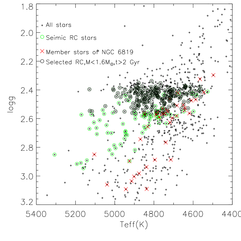
Figure 1: $T_{\rm{eff}}$ versus log(g) diagrams for all stars in SAGA (open diamonds), highlighting stars seismically identified as RC (green open circles), members of the young open cluster NGC 6819 (red crosses), and seismically identified RCs with $M<1.6$ $M_{\sun}$ and age $>2$ Gyr (black open circles).

3 Color and magnitude calibrations in different photometric systems

In addition to our Strömgren observations, magnitudes in the following photometric systems are also available for most of the targets: $BV$ and $g^{\prime}r^{\prime}i^{\prime}$ from APASS (Henden et al., 2009), $griz$ from the Kepler Input Catalog (KIC, Brown et al., 2011), $JHK_{s}$ from 2MASS (Cutri et al., 2003) and $W1W2W3$ from WISE (Wright et al., 2010). All seismic targets have apparent magnitudes in the range $10\lesssim V\lesssim 14$, meaning that photometric errors are usually small in all of the above systems, with typical uncertainties varying between $0.01$ and $0.03$ mag. We discuss each photometric system and the quality cuts adopted on the photometry in the following sub-sections.

Before doing this though, reddening must be properly taken into account to derive correct intrinsic colors and absolute magnitudes. SAGA provides reddening $E(B-V)$ for all asteroseismic targets. We use these values to deredden all photometric measurements, using extinction coefficients appropriate for clump stars. These are computed as described in Casagrande & VandenBerg (2014); briefly, we apply the Cardelli et al. (1989) extinction law to a synthetic spectrum representative of clump stars ($\mbox{\rm$T_{\rm{eff}}$}=4750\,K$, $logg=2.0$ and $\mbox{\rm[Fe/H]}=0$) from which the following coefficients are derived: $R_{B}=3.934$ and $R_{V}=3.086$ for the Johnson system, $R_{g}=3.669$, $R_{r}=2.687$, $R_{i}=2.106$ and $R_{z}=1.517$ for the Sloan $griz$ system, $R_{b}=3.846$ and $R_{y}=3.124$ for the Strömgren system, $R_{J}=0.894$, $R_{H}=0.566$ and $R_{K_{S}}=0.366$ for the 2MASS system, and $R_{W1}=0.242$, $R_{W2}=0.134$ and $R_{W3}=0.349$ for the WISE system. These values are consistent with those published in the literature, but have the advantage of being computed using a reference spectrum appropriate for RCs, thus ensuring better consistency among different bands.

Once color excess and extinction coefficients are know, dereddened magnitudes in any given band $\zeta$ can be derived as $m_{\zeta,0}=m_{\zeta}-R_{\zeta}E(B-V)$, from which dereddened absolute magnitudes $M_{\zeta,0}=m_{\zeta,0}-5\log D+5$, where $D$ is the distance (in parsec), also determined from SAGA. Distances in SAGA are obtained scaling angular diameters computed via the InfraRed Flux Method to asteroseismic radii. The distance of each star is then fed into empirically calibrated, three dimensional Galactic extinction models to derive its reddening, with an iterative procedure to converge in both distance and reddening. Individual uncertainties on reddening are not available, but those are expected to be of order $\pm 0.02$ mag on average (Casagrande et al., 2014a), given that the SAGA sample used here covers a stripe with Galactic latitude between $8^{\circ}$ and $20^{\circ}$, where reddening is relatively low. Thus, the average colors of stars vary by considerable less than this uncertainty. Further, the zero point of our reddening values is anchored to the open cluster NGC 6819 for which a robust value of $E(B-V)=0.14\pm 0.01$ is available from the literature. On average, reddening uncertainties are thus at the level of few hundredths of a magnitude, having negligible impact on the color–absolute magnitude calibrations presented later in the paper.

As a further check on the reddening values adopted from SAGA, we also derive independent estimates using the relation $E(B-V)=A_{K_{s}}/0.366=0.918(H-W2-0.08)/0.366$, where the expression for $A_{K_{s}}$ is based on the Rayleigh-Jeans Color Excess method (RJCE, Majewski et al., 2011). This technique relies on the near-constancy of the infrared color $H-$[4.5$\mu$m]) for evolved stars. In our case we adopt $H$ and $W2$ magnitudes from 2MASS and WISE, respectively. The latter filter is centred on a wavelength of 4.6$\mu$m which is taken into account by the $-0.08$ factor in $A_{K_{s}}$ as reported in Majewski et al. (2011).

As an example of the different precision achieved with different sets of reddening values, Fig. 2 shows the $(b-y)$ vs. $M_{y}$ relation for RCs when adopting $E(B-V)$ from SAGA or the RJCE calibration instead. In the latter case, the scatter of the color–absolute magnitude relation is considerably larger (0.14 vs. 0.10). In particular, stars belonging to the open cluster NGC 6819 cover a broad range of colors, whereas when switching to the reddening values from SAGA it narrows around $(b-y)\simeq 0.63$.

In this paper linear fits are obtained using the IDL linear regression routine regress. Uncertainties stemming from photometric and distance errors are taken into account in doing the fits. For each fit we also compute the Pearson and Spearman coefficients to measure the strength of correlations. Results from this method are labeled as IDL-reg in what follows. To check the robustness of our results to potential outliers, we also employ two additional methods. One method models outliers using a mixture model consisting of a straight line, mixed with a broad Gaussian to capture outliers. We adapted the Python code exMix1 of Hogg, Bovy & Lang (2010) and label the results from this method as Py-exMix1. The other method performs a robust linear regression using an M estimator, by employing iterated re-weighted least squares, as implemented in the R function rlm; we label results using this method as R-rlm.

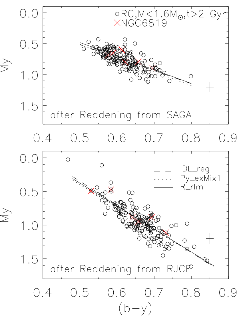
Figure 2: The $(b-y)$ versus $M_{y}$ diagrams for RC stars based on reddening from the SAGA (top panel) and the RJCE method (bottom panel). Seismically identified members of the open cluster NGC 6819 are shown by crosses. Stars with photometric errors in either $b$ or $y$ larger than $0.03$ mag are excluded. Linear fits based on three methods (see description in the text) are shown by dash (IDL-reg), dot (Py-exMix1) and solid (R-rlm) lines, respectively. All colors and magnitudes are corrected for reddening.

3.1 Strömgren

As shown in Fig. 2, the bulk of RCs cover the color range $0.50\lesssim(b-y)\lesssim 0.75$ mag and have absolute magnitudes between $0.4\lesssim M_{y}\lesssim 1.1$ mag. Clearly, $M_{y}$ has a steep dependence on $(b-y)$ color, which we linearly fit (IDL-reg) obtaining the following relation $M_{y}=2.209(b-y)-0.626$ ($\sigma=0.10$) using 162 RCs with good quality data. Note that stars with photometric errors in either $b$ or $y$ larger than $0.03$ mag are excluded here. The relations of $M_{y}=2.206(b-y)-0.620$ from R-rlm method and of $M_{y}=2.220(b-y)-0.613$ from Py-exMix1 are very close to the IDL-reg results, and agree within the scatter. Both the Pearson and Spearman coefficients are 0.72, indicating a strong correlation.

When the metallicity is taken into account, we find $M_{y}=2.097(b-y)+0.045[Fe/H]-0.532$ ($\sigma=0.102$) based on IDL-reg. Generally, RC stars in our sample have a metallicity range of $-0.5<\mbox{\rm[Fe/H]}<0.5$, which corresponds to a variation of $\lesssim 0.04\,$mag in $M_{y}$. This variation is smaller than the scatter of the $M_{y}$ calibration. Thus, in the following of the work we only provide calibrations linking absolute magnitudes to colors. We also explored whether introducing a second order term in color improved upon the residual of our fit, but find this not to be the case. In fact, the major source of uncertainty in our calibration is represented by a mean uncertainty of $0.08\,$mag in absolute magnitudes as a consequence of our typical distance uncertainties.

3.2 Johnson

Fig. 3 shows the $(B-V)$ versus $M_{V}$ diagram, and the absolute magnitude distributions in Johnson system for RC stars. In the Johnson $BV$ system, stars with APASS measurement uncertainties larger than $0.05\,$mag in either $B$ or $V$ band are removed. Most RCs are located in the range $0.6\lesssim(B-V)\lesssim 1.3\,$mag and $0.5\lesssim M_{V}\lesssim 1.0\,$mag. Based on 119 stars, the scatter is $0.15\,$mag. A more strict limit on the measured errors of less than $0.03\,$mag in either B or V band does not improve the correlation and the star number of the sample is reduced to 53 stars. This scatter likely reflects the quality of the APASS magnitudes (see also next Section). Note that fits to the color and absolute magnitude relation based on the three methods,IDL-reg, Py-exMix1 and R-rlm are quite similar. The Pearson (Spearman) correlation is 0.13 (0.18), indicating a weak correlation between absolute magnitude and color, as already apparent from Fig. 3.

Figure 3: The $(B-V)$ versus $M_{V}$ and the color and absolute magnitude distributions in Johnson system, for our sample stars. All colors and magnitudes are corrected for reddening.

3.3 Sloan

Magnitudes in the $griz$ system are available from the Kepler Input Catalog, with typical uncertainties of $0.02$ mag (Brown et al., 2011). However, KIC magnitudes are not exactly on the Sloan system, and thus have been corrected with the transformations provided by Pinsonneault et al. (2012). In addition, for a large fraction of stars $g^{\prime}r^{\prime}i^{\prime}$ magnitudes are also available from the APASS survey; these are defined in the primed system and thus have been converted into the Sloan system using the transformations of Tucker et al. (2006). However, we also note that in the color–absolute magnitude plane the scatter is larger when using APASS magnitudes instead of KIC, thus pointing to lower precision for the former measurements. Therefore, in the following of the analysis we will use only KIC $griz$ magnitudes.

Fig. 4 shows the color–absolute magnitude diagrams in different bands. A few stars are marked with red crosses, and removed from the rest of the analysis: they are somewhat offset from the bulk of other stars, and have been identified as anomalous from their 2MASS colors (see next Section). Absolute magnitudes in each $griz$ band vary linearly with colors, and their slopes flatten moving to filter centered at longer wavelengths, i.e. from $M_{g}$ to $M_{z}$. Two stars with $(g-r)>1.0$ seem to deviate from the linear trend of $M_{g}$ versus $(g-r)$. The number of points is too little to draw further conclusions, however we advise caution from using the the calibration at $(g-r)>1.0$. Panels in Fig. 4 display a correlation between colors and absolute magnitudes which vary depending on the filter, and decreases as moving to redder filters (see Table 1 for a list of Pearson and Spearman coefficients). We also note that the decrease of $M_{i}$ with $(r-i)$ is consistent with the result of Zhao et al. (2001) who found a dependence of Johnson $M_{I}$ with $(V-I)$. Chen et al. (2009) suggested that $i$ and $z$ are the best bands for distance calibration of red clump/red horizontal branch stars in the Sloan system. Here we find that $M_{g}$ versus $(g-r)$ provides an equally good distance calibration.

Figure 4: Color and absolute magnitude diagrams and their distributions in the Sloan $griz$ system for our sample stars. Red crosses identify infrared anomalous stars as described in Section 3.4 and Figure 5. All colors and magnitudes are corrected for reddening.

3.4 2MASS

We restrict ourself to stars with $JHK_{s}$ errors less than $0.03\,$ mag. Fig. 5 shows the $(J-H)$ versus $M_{J}$; $(J-H)$ versus $M_{H}$; $(H-K_{s})$ versus $M_{H}$ and $(J-K_{s})$ versus $M_{K_{s}}$ diagrams, as well as the 2MASS color and absolute magnitude distributions for our sample stars. There is a mild slope in $M_{J}$ as a function of color $(J-H)$, while in the two remaining filters $M_{H}$ and $M_{K_{s}}$ there is almost no trend with color. This is quantified in Table 1 with the Pearson and Spearman correlation coefficients.

In the widely used diagram of $(J-K_{s})$ versus $M_{K_{s}}$, RC stars cover the color range $0.5-0.7\,$mag, and most of them cluster at an absolute magnitude that is consistent with the value $M_{K_{s}}=-1.613$ obtained by Laney et al. (2012) using local RC stars (indicated in the figure with a solid line). Note that the value in Laney et al. (2012) is already converted into the 2MASS system, thus allowing direct comparison with our results.

Figure 5: Colour–absolute magnitude diagram of RC stars in various combination of 2MASS filters. The solid line in the $(J-K_{s})$ versus $M_{K_{s}}$ diagram is the absolute magnitude of local RC stars from Laney et al. (2012). Dashed lines indicate $\pm 0.15\,$mag with respect to the absolute magnitude of local red clump stars, as explained in the text. Stars beyond the dashed lines are marked by red crosses. Bottom panels: absolute magnitude and color distributions for our sample of stars in the 2MASS system. All colors and magnitudes are corrected for reddening.

For some stars, color and absolute magnitude combinations in the infrared show significant deviations from the mean values of the whole sample, which is not compatible with the maximum allowed photometric errors of $0.03\,$mag set here, even after taking into account reddening and distance uncertainties on absolute magnitudes. Specifically, ten stars marked by red crosses in Fig. 5 lie beyond the dashed lines, which represent a deviation of $0.15\,$mag (typical maximum error) from the absolute magnitude $M_{K_{s}}=-1.613$ obtained by Laney et al. (2012) from local RC stars. The quoted 2MASS $JHK_{s}$ errors for the these stars can not explain such large deviations. Most of these deviant stars are overluminous, and this would point towards the presence of some sort of infrared emission e.g., due to a hot circumstellar disk. Also, although we have removed RC stars with ages below 2 Gyr from our analysis, five of the deviant ones have ages between 2 and 3 Gyr, and thus some residual age effect on absolute magnitudes could still be present for some of these objects. Investigating these scenarios however is beyond the scope of the present paper. We exclude these stars in the rest of the analysis, and we mark them with red crosses in the plots for reference.

3.5 WISE

Fig. 6 shows the color–absolute magnitude diagrams in the WISE system. Photometric uncertainties in $W1W2$ are of order $0.02$ mag, significantly smaller than for $W3W4$, which are of order $0.02-0.10$ and $0.10-0.50$ mag, respectively. Because of these uncertainties, we impose a threshold on the maximum allowed photometric error: $0.03$ mag on $W1$ and $W2$, and $0.05$ mag on $W3$, while we discard $W4$ from the rest of the analysis.

The color and magnitude ranges in the WISE system are quite small, which indicates that these bands can be used to obtain very good distances for RC stars. We quantify in Table 1 the Pearson and Spearman correlation coefficients. Also, comparing Fig 4, 5 and 6 we see that the slope of absolute magnitudes as function of colors flattens out, and then reverses as moving to longer wavelength.

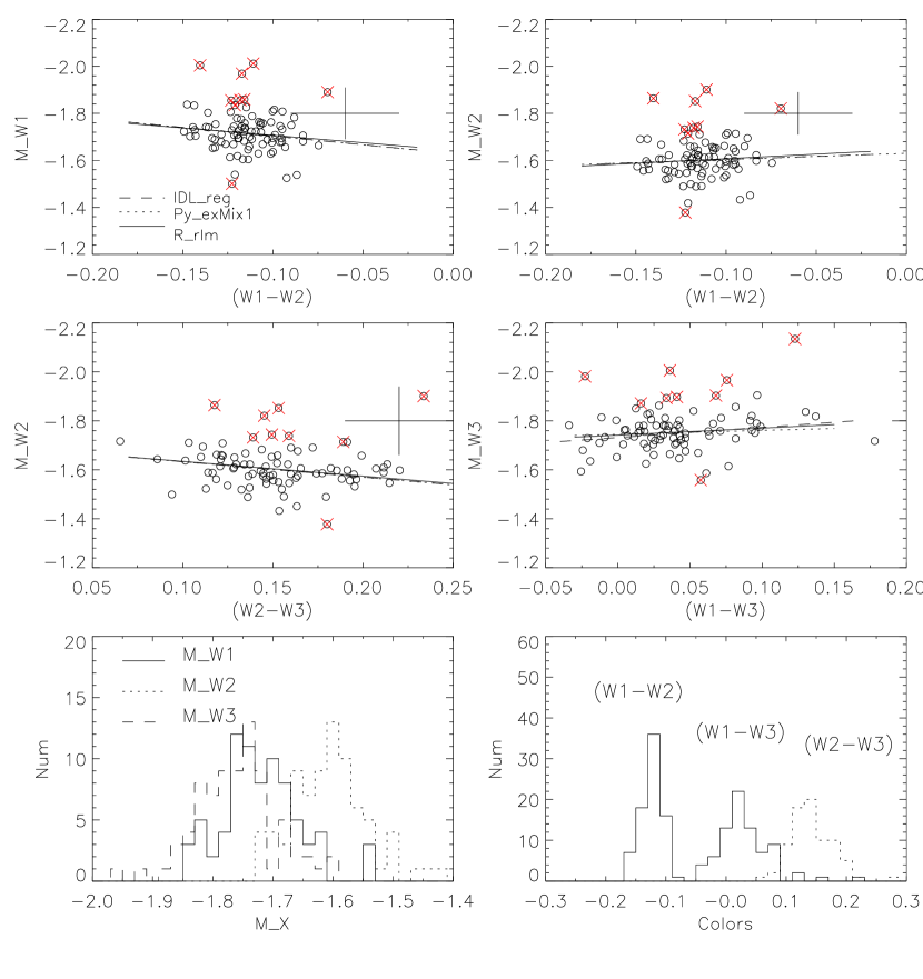
Figure 6: Color–absolute magnitude diagrams in various combinations of WISE filters for our sample of stars. Red crosses same as in Fig. 5. All colors and magnitudes are corrected for reddening.

Table 1: Mean colors and absolute magnitudes, together with the color-absolute magnitude calibrations and Pearson/Spearman correlation coefficients based on IDL-reg function, in different photometric systems for RC stars. Difference between mean and median values is usually a few millimag only, and never exceed $0.01\,mag$. We use the scatter of the data as a conservative estimate of the errors: if we were to use the standard deviation of the mean, uncertainties would be a factor of 10 smaller. Note that all colors and absolute magnitudes are corrected for reddening.

$(b-y)=0.619\pm 0.048$	$M_{y}=0.754\pm 0.147$	$M_{y}=2.209(b-y)-0.626$	$0.72/0.72$
$(B-V)=1.025\pm 0.140$	$M_{V}=0.735\pm 0.148$	$M_{V}=0.189(B-V)+0.525$	$0.13/0.18$
$(g-r)=0.809\pm 0.078$	$M_{g}=1.229\pm 0.172$	$M_{g}=2.010(g-r)-0.402$	$0.88/0.89$
$(g-r)=0.809\pm 0.078$	$M_{r}=0.420\pm 0.110$	$M_{r}=1.010(g-r)-0.402$	$0.67/0.72$
$(r-i)=0.263\pm 0.029$	$M_{r}=0.420\pm 0.110$	$M_{r}=2.738(r-i)-0.303$	$0.65/0.71$
$(r-i)=0.263\pm 0.029$	$M_{i}=0.157\pm 0.094$	$M_{i}=1.738(r-i)-0.303$	$0.45/0.55$
$(i-z)=0.136\pm 0.021$	$M_{i}=0.157\pm 0.094$	$M_{i}=2.382(i-z)-0.169$	$0.53/0.52$
$(i-z)=0.136\pm 0.021$	$M_{z}=0.022\pm 0.084$	$M_{z}=1.382(i-z)-0.169$	$0.34/0.34$
$(J-H)=0.513\pm 0.034$	$M_{J}=-1.016\pm 0.063$	$M_{J}=0.975(J-H)-1.518$	$0.50/0.47$
$(H-K_{s})=0.097\pm 0.024$	$M_{H}=-1.528\pm 0.055$	$M_{H}=0.494(H-K_{s})-1.580$	$0.15/0.18$
$(J-K_{s})=0.609\pm 0.040$	$M_{K_{s}}=-1.626\pm 0.057$	$M_{K_{s}}=-0.188(J-K_{s})-1.517$	$-0.17/-0.09$
$(y-K_{s})=2.383\pm 0.129$	$M_{K_{s}}=-1.626\pm 0.057$	$M_{K_{s}}=-0.003(y-K_{s})-1.625$	$-0.03/0.08$
$(W1-W2)=-0.112\pm 0.016$	$M_{W1}=-1.694\pm 0.061$	$M_{W1}=0.612(W1-W2)-1.632$	$0.17/0.13$
$(W2-W3)=0.155\pm 0.043$	$M_{W2}=-1.595\pm 0.064$	$M_{W2}=0.628(W2-W3)-1.696$	$0.25/0.23$
$(W1-W3)=0.043\pm 0.044$	$M_{W3}=-1.752\pm 0.068$	$M_{W3}=-0.307(W1-W3)-1.741$	$-0.36/-0.20$
$(H-W2)=0.053\pm 0.025$	$M_{W2}=-1.581\pm 0.060$	$M_{W2}=-0.967(H-W2)-1.533$	$-0.41/-0.36$

Table 2: The color–absolute magnitude calibrations based on R-rlm function for RC stars. Note that all colors and absolute magnitudes are corrected for reddening.

$M_{y}=2.206(\pm 0.149)(b-y)-0.620(\pm 0.093)$

$M_{V}=0.200\pm 0.096)(B-V)+0.512(\pm 0.099)$

$M_{g}=2.099(\pm 0.089)(g-r)-0.463(\pm 0.072)$

$M_{r}=1.109(\pm 0.089)(g-r)-0.467(\pm 0.071)$

$M_{r}=3.117(\pm 0.238)(r-i)-0.399(\pm 0.059)$

$M_{i}=2.116(\pm 0.239)(r-i)-0.390(\pm 0.059)$

$M_{i}=1.752(\pm 0.257)(i-z)-0.058(\pm 0.038)$

$M_{z}=0.753(\pm 0.316)(i-z)-0.057(\pm 0.038)$

$M_{J}=1.011(\pm 0.129)(J-H)-1.534(\pm 0.066)$

$M_{H}=0.536(\pm 0.171)(H-K_{s})-1.580(\pm 0.017)$

$M_{K_{s}}=-0.106(\pm 0.104)(J-K_{s})-1.560(\pm 0.063)$

$M_{K_{s}}=0.045(\pm 0.031)(y-K_{s})-1.740(\pm 0.077)$

$M_{W1}=0.631(\pm 0.426)(W1-W2)-1.643(\pm 0.049)$

$M_{W2}=0.601(\pm 0.175)(W2-W3)-1.694(\pm 0.028)$

$M_{W3}=-0.289(\pm 0.166)(W1-W3)-1.742(\pm 0.010)$

$M_{W2}=-0.854(\pm 0.197)(H-W2)-1.538(\pm 0.011)$

3.6 The Combined Strömgren, 2MASS and WISE Systems.

It is interesting to explore two widely used combination of color and absolute magnitudes for RC stars. Namely, $(V-K_{s})$ versus $M_{K_{s}}$ and $(H-W2)$ versus $M_{W2}$ are widely adopted in the literature. Since $V$ magnitudes in APASS have somewhat large errors, we adopt $y$ magnitudes in this analysis (where in fact, Strömgren $y$ was historically defined to be essentially the same as Johnson $V$). Fig. 7 shows the $(y-K_{s})$ versus $M_{K_{s}}$, and the $(H-W2)$ versus $M_{W2}$ diagrams, together with their color distributions. There is essentially flat correlation between $(y-K_{s})$ and $M_{K_{s}}$, with a Pearson (Spearman) coefficient of $-0.03$ (0.08). On the contrary, $M_{W2}$ inverse correlates with $(H-W2)$, the Pearson (Spearman) coefficient being $-0.41$ ($-0.36$). Color histograms are shown in the bottom of Fig. 7, and the mean values are $(y-K_{s})=2.383\pm 0.129$ and $(H-W2)=0.053\pm 0.025$. In particular, the rather narrow range of $(H-W2)$ makes it a useful cryon to determine reddening in high extinction areas using RC stars.

Our results based on IDL-reg function are summarized in Table 1. Results from PYTHON exMix1 and R-rlm are very close, and we present the color–absolute magnitude calibrations based on R-rlm function in Table 2.

Figure 7: Color–absolute magnitude diagram for RC in the $(y-K_{s})$ versus $M_{K_{s}}$ and $(H-W2)$ versus $M_{W2}$ system. Red crosses are the same as in Fig. 5. Bottom panels show the color distributions. All colors and magnitudes are corrected for reddening.

3.7 The age dependence of the distance scale.

Using the age (and mass) information available from SAGA, in Fig. 8 we plot absolute magnitudes of RC stars as function of age, in the $K_{s}$ and $W2$ bands, which are two among the filters displaying the least colour-dependence. Stars with age errors larger than 30% are removed from this plot, although they would still follow the same trend if included. Interestingly, older than $2$ Gyr there is a clear dependence of $K_{s}$ and $W2$ absolute magnitudes on age. Fitting this trend with IDL-reg, we obtain:

$$M_{K_{s}}=(0.015\pm 0.003)\,\tau-1.715(\pm 0.016)$$ (1)

and

$$M_{W2}=(0.017\pm 0.003)\,\tau-1.682(\pm 0.016)$$ (2)

where $\tau$ is the age of RC stars in Gyr. Fits using R-rlm and Py-exMix1 are very similar. $M_{K_{s}}=(0.016\pm 0.002)\,\tau-1.715(\pm 0.008)$, $M_{W2}=(0.018\pm 0.002)\,\tau-1.683$ with the former method and $M_{K_{s}}=(0.015\pm 0.003)\,\tau-1.714$ and $M_{W2}=(0.017\pm 0.004)\,\tau-1.682$ with the latter. The Pearsons (Spearman) correlation coefficients are of 0.65 (0.62) for $M_{K_{s}}$ and 0.66 (0.63) for $M_{W2}$, indicating a strong linear correlations. In Table 3 we report the slope of ages versus magnitudes for all our photometric systems. It has to be kept in mind that certain filters also display color dependence, and thus the interdependence of ages and colors might not be straightforward to disentangle. In general, we can say that for optical colors there is a slope of $\sim 0.030\pm 0.003\,\rm{mag\,Gyr}^{-1}$ whereas in the infrared the dependence is $\sim 0.020\pm 0.003\,\rm{mag\,Gyr}^{-1}$ and it also displays a stronger correlation.

Note that the asteroseismic ages adopted here are obtained assuming no mass-loss. If we were to use instead asteroseismic ages derived assuming a highly efficient mass-loss, the slopes above would increase even further. E.g., the slopes of $M_{K_{s}}$ and $M_{W2}$ would be $\sim 0.031\pm 0.011\,\rm{mag\,Gyr}^{-1}$ and $\sim 0.035\pm 0.011\,\rm{mag\,Gyr}^{-1}$. We refer to Casagrande et al. (2016) for a discussion why a negligible mass-loss is however favored by current observations.

The dependence of absolute magnitudes of RC stars on age is theoretically predicted (see Girardi & Salaris, 2001, in $I$ band) and found in open clusters by Grocholski et al. (2002) using 2MASS photometry. Here, for the first time, we detect such a tiny trend in various optical and infrared bands in field stars thanks to the accuracy of our asteroseismic ages and distances (and hence luminosities).

Figure 8: $M_{K_{s}}$ and $M_{W2}$ as function of stellar ages for different log(g) ranges. Absolute magnitudes are corrected for reddening. Ages below 2 Gyr are plotted only to highlight their wide range of absolute magnitudes, but are not used for the fits. Stars with age error larger than 30% are not shown.

Table 3: Slope of absolute magnitude versus ages in $\rm{mag\,Gyr}^{-1}$ for different filters. Last column indicates Pearson and Spearman correlation coefficients.

band	slope	correlation
$y$	$0.032\pm 0.003$	$0.43/0.43$
$V$	$0.028\pm 0.003$	$0.40/0.41$
$g$	$0.036\pm 0.003$	$0.40/0.42$
$r$	$0.029\pm 0.003$	$0.52/0.50$
$i$	$0.026\pm 0.003$	$0.55/0.53$
$z$	$0.025\pm 0.003$	$0.61/0.60$
$J$	$0.020\pm 0.003$	$0.63/0.62$
$H$	$0.018\pm 0.003$	$0.71/0.69$
$K_{s}$	$0.015\pm 0.003$	$0.65/0.62$
$W1$	$0.016\pm 0.003$	$0.62/0.59$
$W2$	$0.017\pm 0.003$	$0.66/0.63$
$W3$	$0.017\pm 0.004$	$0.51/0.48$

4 Literature comparison: using the distance scale to test asteroseismic scaling relations

In the Johnson system, $M_{V}$ are generally consistent with previous results from Bilir et al. (2013a) based on red clump/red horizontal branch stars in globular and open clusters. They also found a weak metallicity dependence of the $M_{V}$ with a coefficient of $0.046$ added to the magnitude versus $(B-V)$ calibration. The weak dependence of $M_{y}$ on [Fe/H] in our work in the Strömgren system is consistent with the result of Bilir et al. (2013a). The absolute magnitudes of RC stars are calibrated in Bilir et al. (2013b) in terms of colors for $M_{V}$, $M_{J}$, $M_{K_{s}}$ and $M_{g}$. Our color–absolute magnitude diagrams are consistent with those in Bilir et al. (2013b) (their figure 8), although our seismic selection of RC stars results in a smaller scatter. Our mean values of $M_{J}=-1.016\pm 0.063$ and $M_{H}=-1.528\pm 0.055$ agree within the errors with those of Laney et al. (2012) who gave $M_{J}=-0.984\pm 0.014$ and $M_{H}=-1.490\pm 0.015$ based on local RC stars.

The comparison with $M_{K_{s}}$ values from the literature indicates an overall agreement, although it deserves a discussion. Our value of $M_{K_{s}}=-1.626\pm 0.057$ is consistent with that of $-1.613\pm 0.015$ by Laney et al. (2012) for local RC stars, and that of $-1.61\pm 0.04$ by Grocholski et al. (2002) for RC stars in clusters. The values of $-1.57\pm 0.05\,$mag by van Helshoecht & Groenewegen (2007) and of $-1.54\pm 0.04\,$mag by Groenewegen (2008) for local RC stars with Hipparcos parallaxes are fainter than our value. The comparison of our values of $M_{W1}=-1.694\pm 0.061$ and $M_{W3}=-1.752\pm 0.068$ with those of $M_{W1}=-1.635\pm 0.026$ and $M_{W3}=-1.606\pm 0.024$ in Yaz Gökçe et al. (2013) shows deviations of $-0.06\,$mag in $M_{W1}$ and $-0.15\,$mag in $M_{W3}$ (ours minus theirs, our absolute magnitudes being brighter). Yaz Gökçe et al. (2013) also provide $M_{J}$, $M_{H}$ and $M_{K_{s}}$, and again our absolute magnitudes are brighter by $\simeq-0.03$ to $-0.06$ mag. From the above comparisons, we conclude that differences with the Hipparcos literature are generally within the errors, although it is intriguing to notice that they seem systematic, in the sense that our absolute magnitudes are brighter.

Our absolute magnitudes are based on seismic distances $D$, which are derived scaling angular diameters obtained via the InfraRed Flux Method to the stellar radii $R$ obtained from scaling relations (Silva Aguirre et al., 2012; Casagrande et al., 2014a). We have carried out an extensive comparison of our angular diameters with interferometric measurements in Casagrande et al. (2014b). If we assume our angular diameter scale to be correct, then any change in stellar radii due to scaling relation directly translates into a change of distances. Thus, we can compare the absolute magnitude of clump stars we derive (i.e. based on distances relying on scaling relations) with those available in the literature and obtained with independent methods. From distance modulus, it follows that for a given photometric system a difference $\Delta M=M-M_{l}$ in absolute magnitudes between our calibrations ($M$) and those available in the literature $M_{l}$ corresponds to a fractional change in distance

$$\frac{D}{D_{l}}=10^{-0.2\Delta M}$$ (3)

which can then be used to constrain how much seismic radii $R$ should vary to agree with the distance scale in the literature. In this way, we can thus put an upper limit to the precision of scaling relations.

For this purpose, we compare the difference of the absolute magnitudes with those in the literature for $M_{K_{s}}$, the filter showing the least dependence on colors, and only mildly affected by reddening. The offsets are $-0.013$ mag with respect to the absolute magnitude in Laney et al. (2012), $-0.056$ mag with respect to van Helshoecht & Groenewegen (2007), $-0.086$ mag with respect to Groenewegen (2008) and $-0.016$ mag with respect to Grocholski et al. (2002). This corresponds to our seismic distances being $10^{-0.2\Delta M}$, i.e. $1.006$, $1.026$, $1.040$ and $1.007$ larger. If we assume that radii from scaling relation are entirely responsible for the difference, then radii from scaling relations are overestimated by an amount that goes from $0.6\pm 2.7\%$ to $4.0\pm 3.2\%$ depending on the literature calibration we compare with. The average offset is $2\pm 2\%$. This comparison indicates a mild tension between our seismic distance scale, and that deduced from Hipparcos parallaxes. If confirmed, it would put a limit to the accuracy at which scaling relations are applicable to red clump stars. However, a few caveats must be remembered. Our comparison assumes no color dependence (i.e. we only compare mean absolute magnitudes). Also, one may wonder whether the age distribution underlying our sample is different from that of other calibrations. Since all calibrations are based on nearby stars, or open clusters, it is reasonable to assume that the underlying age distributions are comparable. However, calibrations using field stars in the literature have no age information, and likely include many stars younger than 2 Gyr, which instead we have excluded. If we were to include stars of all ages in our calibration, the mean absolute magnitude for our sample would be $M_{K_{s}}=-1.628\pm 0.130$, i.e. the difference would stay the same, but the scatter would increase significantly.

5 Summary

Based on the reddening and distance estimates for a sample of $\sim 170$ seismically identified red clump stars in Casagrande et al. (2014a), we have investigated color and absolute magnitude distributions of RC stars in Strömgren $by$, Johnson $BV$, Sloan $griz$, 2MASS $JHK_{s}$ and WISE $W1W2W3$ photometric systems. For the first time, we find a clear trend between absolute magnitudes and ages in field RC stars. The absolute magnitudes of RC stars deviate significantly from a constant value at ages below 2 Gyr, which indicates that RC stars can be reliably used as distance indicators only for populations older than this age. Even so, a statistically significant correlation between absolute magnitudes and ages remain, which in worst case can introduce a bias up to $\sim 0.3\,$mag in the optical and $\sim 0.2\,$mag in the infrared if ages of clump stars are not known. Our absolute magnitudes for RC stars in the 2MASS and WISE system are generally consistent within the errors with those obtained from local RC stars with accurate Hipparcos parallaxes. However, a possible tension at the level of a few percent is identified. Assuming that seismic scaling relations are responsible for this difference, this would imply that seismic radii for red clump stars are overestimated by $2\pm 2\%$ when using scaling relations. Our methodology, along with improvements on the calibration of the distance scale with future Gaia data releases will be able to shed light on this issue.

References

- Auvergne et al. (2009) Auvergne M et al., 2009, A&A, 506, 411
- Basu et al. (2011) Basu S. et al., 2011, ApJ, 729, L10
- Bedding et al. (2011) Bedding, T.R. et al., 2011, Natur, 471, 608
- Bilir et al. (2013a) Bilir, S., Ak, T., Ak, S., Yontan, T., Bostanc, Z.F., 2013a, NewA, 23, 88
- Bilir et al. (2013b) Bilir, S., Onal, O., Karaali, S., Cabrera-Lavers, A., Cakmak, H., 2013b. Ap&SS, 344, 417
- Brogaard et al. (2016) Brogaard, K., Jessen-Hansen, J., Handberg, R., et al. 2016, Astronomische Nachrichten, 337, 793
- Brown et al. (2011) Brown, T. M., Latham, D. W., Everett, M. E., & Esquerdo, G. A. 2011, AJ, 142, 112
- Calamida et al. (2014) Calamida A., Bono G., Lagioia E.P. et al. 2014, A&A, 565, 8
- Cannon (1970) Cannon, R.D.: 1970, MNRAS, 150, 111
- Cardelli et al. (1989) Cardelli, J. A., Clayton, G. C., & Mathis, J. S. 1989, ApJ, 345, 245
- Casagrande & VandenBerg (2014) Casagrande, L., & VandenBerg, D. A. 2014, MNRAS, 444, 392
- Casagrande et al. (2014a) Casagrande, L., Silva Aguirre, V., Stello, D., et al. 2014a, ApJ, 787, 110
- Casagrande et al. (2014b) Casagrande, L., Portinari, L., Glass, I. S., et al. 2014b, MNRAS, 439, 2060
- Casagrande et al. (2016) Casagrande, L., et al. 2016, MNRAS, 455, 987
- Chen et al. (2009) Chen, Y. Q., Zhao, G., Zhao, J. K. 2009 ApJ,702,1336
- Cutri et al. (2003) Cutri, R. M., Skrutskie, M. F., van Dyk, S., et al. 2003, ”The IRSA 2MASS All-Sky Point Source Catalog, NASA/IPAC Infrared Science Archive.”
- Dutra et al. (2002) Dutra, C. M.; Santiago, B. X.; Bica, E. 2002, A&A, 381, 219
- Gaulme et al. (2016) Gaulme, P., McKeever, J., Jackiewicz, J., et al. 2016, ApJ, 832, 121
- Gilliland et al. (2010) Gilliland R.L. et al., 2010, PASP, 122, 131
- Girardi (1999) Girardi L., 1999, MNRAS, 308, 818
- Girardi et al. (1998) Girardi L., Groenewegen M. A. T., Weiss A., Salaris M., 1998, MNRAS, 301, 149
- Girardi et al. (2000) Girardi L., Mermilliod J.-C., Carraro G., 2000, A&A, 354, 892
- Girardi & Salaris (2001) Girardi L. & Salaris M., 2001, MNRAS, 323, 109
- Groenewegen (2008) Groenewegen, M.A.T.: 2008, A&A, 488, 25
- Grocholski et al. (2002) Grocholski, A.J., Sarajedini, A., 2002, AJ, 123, 1603
- Hekker et al. (2011) Hekker S. et al., 2011a, A&A, 530, A100
- Henden et al. (2009) Henden, A. A., Welch, D. L., Terrell, D., & Levine, S. E. 2009, American Astronomical Society Meeting Abstracts #214, 214, #407.02
- Hesser & Hartwick (1977) Hesser, J.E. & Hartwick, F.D.A, 1977, ApJS, 33, 361
- Hogg, Bovy & Lang (2010) Hogg, D.W., Bovy, J., & Lang D. astro-ph/1008.4686v1
- Huber et al. (2010) Huber D. et al., 2010, ApJ, 723, 1607
- Huber et al. (2012) Huber, D., Ireland, M. J., Bedding, T. R., et al. 2012, ApJ, 760, 32
- Huber et al. (2014) Huber, D., Silva Aguirre, V., Matthews, J. M., et al. 2014, ApJS, 211, 2
- Iben (1968) Iben, I. 1968, Nature, 220, 143
- Lindegren et al. (2016) Lindegren, L., Lammers, U., Bastian, U., et al. 2016, A&A, 595, A4
- Karaali et al. (2013) Karaali, S., Bilir, S., & Yaz Gökçe, E. 2013, Ap&SS, 346, 89
- King et al. (1985) King, C. R., Da Costa, G. S., & Demarque, P. 1985, ApJ, 299, 674
- Laney et al. (2012) Laney, C.D., Joner, M.D., Pietrzyński, G., 2012. MNRAS 419, 1637
- Lasker et al. (2008) Lasker, B. M., Lattanzi, M. G., McLean, B. J., et al. 2008, AJ, 136, 735
- Majewski et al. (2011) Majewski, Steven R.; Zasowski, Gail; Nidever, David L. 2011, ApJ, 739, 25
- Mermilliod et al. (1998) Mermilliod J.-C., Mathieu R. D., Latham D. W., Mayor M., 1998, A&A, 339, 423
- Miglio et al. (2009) Miglio, A., Montalbán, J., Baudin, F., et al. 2009, A&A, 503, L21
- Miglio et al. (2013) Miglio, A., Chiappini, C., Morel, T., et al. 2013, MNRAS, 429, 423
- Miglio et al. (2013) Miglio, A., Chiappini, C., Morel, T., et al. 2013, European Physical Journal Web of Conferences, 43, 03004
- Montalbán et al. (2010) Montalbán, J et al. 2010, ApJL 721, 182
- Montalbán et al. (2013) Montalbán, J et al. 2013, ApJ 766, 118
- Paczyński & Stanek (1998) Paczyński B. & Stanek K. Z., 1998, ApJ, 494, 219
- Pinsonneault et al. (2012) Pinsonneault, M. H., An, D., Molenda-Żakowicz, J., et al. 2012, ApJS, 199, 30
- Rodrigues et al. (2014) Rodrigues, T. S., Girardi, L., Miglio, A., et al. 2014, MNRAS, 445, 2758
- Silva Aguirre et al. (2012) Silva Aguirre, V., Casagrande, L., Basu, S., et al. 2012, ApJ, 757, 99
- Skrutskie et al. (2006) Skrutskie M. F. et al., 2006, AJ, 131, 1163
- Stanek & Garnavich (1998) Stanek, K. Z. & Garnavich, P. M., 1998, ApJ, 503, 131
- Stello et al. (2009) Stello, D., Chaplin, W.J., Basu, S., Elsworth, Y., & Bedding, T. R. 2009, MNRAS, 400, L80
- Stello et al. (2013) Stello, D., Huber, D., Bedding, T. R., et al. 2013, ApJ, 765, L41
- Thomas (1967) Thomas, H.-C. 1967, Z. Astrophys., 67, 420
- Tucker et al. (2006) Tucker, D. L., Kent, S., Richmond, M. W., et al. 2006, Astronomische Nachrichten, 327, 821
- van Helshoecht & Groenewegen (2007) van Helshoecht, V., Groenewegen, M.A.T.: 2007, A&A, 463, 559
- White et al. (2011) White, T. R., Bedding, T. R., Stello, D., et al. 2011, ApJ, 743, 161
- White et al. (2013) White, T. R., Huber, D., Maestro, V., et al. 2013, MNRAS, 433, 1262
- Wright et al. (2010) Wright, E.L., et al., 2010. AJ 140, 1868
- Yaz Gökçe et al. (2013) Yaz Gökçe, E., Bilir, S., Öztürkmen, N. D., et al. 2013, New A, 25, 19
- Zhao et al. (2001) Zhao, G., Qiu, H.M., & Mao, S.D., 2001, ApJ, 551, L85
- (62)