Solitons supported by singular modulation of the cubic nonlinearity

Abstract

A model of the optical media with a spatially structured Kerr nonlinearity is introduced. The nonlinearity strength is modulated by a set of singular peaks on top of a self-focusing or defocusing uniform background. The peaks may include a repulsive or attractive linear potential too. We find that a pair of mutually symmetric peaks readily gives rise to the spontaneous symmetry breaking (SSB) of modes pinned to individual peaks, while antisymmetric pinned modes are always unstable, transforming into robust spatially odd breathers. Three- and five-peak structures support symmetric modes, with in-phase or twisted profiles, and do not give rise to asymmetric states. A stability area is found for the twisted states pinned to the triple peaks, while the corresponding in-phase modes are unstable, unless the three modulation peaks are set very close to each other, covered by a single-peak pinned mode. All patterns pinned to five peaks are unstable too. Collisions of moving solitons with the singular-modulation peak are studied too. Slowly moving solitons bounce back from the peak, while the collisions are quasi-elastic for fast solitons. In the intermediate case, the soliton is destroyed by the collision. In a special case, the condition of a resonance of the incident soliton with a trapped mode supported by the peak leads to capture of the soliton.

1 Introduction and the model

The great potential offered by solitons for fundamental studies and development of applications in optics and other areas of physics is commonly known [1, 2, 3, 4, 5]. However, the use of uniform media as a host material for solitons has its limitations, as they admit the existence of few species of solitary modes. In particular, the integrable one-dimensional (1D) setting based on the nonlinear Schrödinger (NLS) equation gives rise to the single stable class of solutions in the form of fundamental solitons [1] (higher-order solutions for breathers are available too [6], but they are not truly stable objects, as their binding energy is zero).

The variety of stable localized objects may be greatly expanded by using pseudopotentials induced by spatial modulation of the local nonlinearity strength [7]. In optics, nonuniform Kerr nonlinearity can be induced by an inhomogeneous distribution of nonlinearity-enhancing dopants [8]. Similar patterns may be realized in composite media assembled of different materials [9, 10, 11, 12]. Still broader flexibility of nonlinearity landscapes is available in Bose-Einstein condensates (BECs), where the landscapes, underlain by the optical Feshbach resonance [13, 14, 15], can be “painted” by rapidly moving laser beams [16, 17]. The magnetic Feshbach resonance can be used too, imposing stationary nonlinearity patterns by means of magnetic lattices [18, 19, 20].

In particular, structures in the form of a very narrow region with strong local cubic nonlinearity, embedded into a linear host setting, are modeled by the NLS equation with a delta-functional coefficient in front of the nonlinear term, $g(x)\sim\delta(x)$ [21, 22, 23, 24, 25] (a discrete version of this setting is represented by a linear dynamical lattice with an embedded  nonlinear site [26, 27, 28, 29]). In this limit, the family of solitons pinned to the point-like inhomogeneity (nonlinear defect) is degenerate, in the sense that their norm does not depend on the propagation constant/chemical potential, in terms of optics and BEC, respectively [23]. The norm degeneracy is a distinctive feature of Townes solitons, such as those supported by uniform cubic [30, 31, 32] and quintic [33] self-focusing in the 2D and 1D geometry, respectively. The fact that solitons of the Townes type are always made unstable by the occurrence of the critical collapse in the same setting makes it necessary to replace the delta-functional nonlinearity profile by more realistic singular ones, approximated by the cusp,

$$g(x)\sim|x|^{-\alpha},$$ (1)

with $\alpha>0$ [34]. The analysis has produced stable solitons pinned to this nonlinearity peak in the range of $0<\alpha<1$. In the limit of $\alpha=1$, the solitons’ amplitude vanishes, and they do not exists at $\alpha>1$, when the singularity is too strong ($\int g(x)dx$ diverges around $x=0$; actually, solitons cannot be pinned to the nonlinearity peak with $\alpha\geq 1$ as they are destroyed by the collapse in that case). It is worthy to note that it was also demonstrated in [34] that the singular modulation profile with $\alpha<1$ may emulate the spatially uniform attractive cubic nonlinearity in a sub-1D space, with effective fractal dimension $D=2\left(1-\alpha\right)/\left(2-\alpha\right)<1$.

A natural continuation of the analysis, which is the objective of the present work, is to study configurations pinned to sets of several nonlinearity peaks. Such patterns can be created in the experiment by means of the same techniques that were proposed for building a single peak. In particular, the possibility of the spontaneous symmetry breaking (SSB) in patterns attached to a pair of identical peaks, which is known in other settings [26, 27, 28, 29], [22, 35], opens a way to use the double peaks for power-controlled switching in optical circuitry. Further, sets of several peaks may be considered as a transition to a periodic lattice of nonlinear defects, which is an object of obvious interest too [36, 37, 38, 39].

Thus, we consider the model based on the NLS equation with an $x$-dependent self-focusing coefficient, $g(x)>0$:

$$iu_{z}=-\frac{1}{2}u_{xx}+\left[\sigma-g(x)\right]{\left|u\right|}^{2}u+\beta g(x)u.$$ (2)

This equation is written in terms of optics, with $z$ and $x$ being the propagation distance and transverse coordinate in a planar waveguide, and $\sigma$ representing the nonlinearity coefficient of the uniform background into which the nonlinearity peaks are embedded. In particular, $\sigma>0$ implies competition of the self-focusing peaks with the self-defocusing background, cf. work [12]. The linear-potential term $\sim\beta$ takes into account the fact that material perturbations, which induce the local modulation of the nonlinearity, may also give rise to similar local changes of the refractive index. In the application to a cigar-shaped trapping configuration in BEC with longitudinal coordinate $x$, the evolutional variable, $z$, in Eq. (2) must be replaced by time $t$, and the term $\sim\beta$ accounts for the local linear potential that may be induced by the same tightly focused laser beams which modify the local strength of the nonlinearity via the Feshbach resonance.

The singular nonlinearity-modulation patterns considered below are specified in Table 1, including two, three, or five peaks. For the completeness’ sake, the single peak, which was introduced in [34], is included too. In these patterns, $\Delta$ determines the separation between adjacent peaks (for the double peak, the separation is $2\Delta$), and $\alpha$ is the singularity power in Eq. (1). Coefficients in front of the singular-modulation functions, which are defined in Table 1, are set to be $1$ by means of obvious rescaling. Further, the remaining scaling invariance may be used to fix $|\sigma|=1$ in Eq. (2), unless we choose $\sigma=0$ (no uniform-nonlinearity background).

It is relevant to stress the difference of the superposition of two singular peaks, defined as per the second line of Table 1, from the superposition of regularized $\delta$-functions, represented by Gaussians with width $a$: while the singular peaks remain discernible at any separation $2\Delta$ between them, the two peaks in the superposition of the Gaussians merge into one at $a/\left(2\Delta\right)>1/\sqrt{2}$ [22].

Table 1: Different sets of nonlinearity-modulation peaks representing the coefficient in front of the cubic term in Eq. (2).

1 peak	$g(x)={\left|x\right|}^{-\alpha}$
2 peak	$g(x)=\left|x-\Delta\right|^{-\alpha}+\left|x+\Delta\right|^{-\alpha}$
3 peak	$g(x)=\left|x-\Delta\right|^{-\alpha}+{\left|x\right|}^{-\alpha}+\left|x+\Delta\right|^{-\alpha}$
5 peak	$g(x)=\left|x-2\Delta\right|^{-\alpha}+\left|x-\Delta\right|^{-\alpha}+{\left|x\right|}^{-\alpha}+\left|x+\Delta\right|^{-\alpha}+\left|x+2\Delta\right|^{-\alpha}$

The rest of the paper is organized as follows. Methods used in the analysis are briefly summarized in Section II. These include a quasi-analytical variational approximation (VA) for the mode pinned to a single peak, and a numerical scheme elaborated for the identification of stationary patterns and their stability. The VA presented here generalizes that from [34], which did not include the linear-potential component of the local peak. Basic results for the SSB in patterns pinned to a pair of peaks are reported in Section III, and findings for the set of three and five peaks (the latter being a prototype of the lattice of nonlinear defects) are presented in Section IV. In Section V, a dynamical situation is considered, viz., collisions of free solitons with a single nonlinearity peak (collisions with defects and interfaces of various types were studied before [40, 41, 42, 43, 44, 45, 46], but not for the present one). The paper is concluded by Section VI.

2 The framework of the analysis

2.1 The variational approximation for a single peak

Stationary solutions to Eq. (2) with propagation constant $k$ are looked for in the usual form, $u\left(x,z\right)=e^{ikz}w(x)$, with real function $w$ satisfying equation

$$kw-\frac{1}{2}w_{xx}+\left[\sigma-g({x})\right]{w}^{3}+\beta g({x})w=0.$$ (3)

Numerical solutions of Eq. (3) with zero boundary conditions at $|x|\rightarrow\infty$ were constructed by means of the Newton’s method, while simulations of the full NLS equation (2) were carried out by means of an explicit Runge-Kutta algorithm. The stationary solutions are characterized by the total power (norm),

$$P=\int_{-\infty}^{+\infty}w^{2}(x)dx.$$ (4)

The use of the Newton’s method is contingent on a possibility to choose a relevant initial guess. It was provided by attaching to each nonlinearity peak a localized mode predicted for the isolated defect by the VA. To this end, the simplest Gaussian ansatz,

$$w(x)=A\exp\left(-\rho x^{2}\right),$$ (5)

is substituted in the Lagrangian of Eq. (3) with $g(x)$ taken as per the top line in Table 1,

$$L=\int_{-\infty}^{+\infty}\left[\frac{1}{4}\left(\frac{dw}{dx}\right)^{2}\right]+\left[\frac{k}{2}w^{2}+\frac{1}{4}\left(\sigma-{\left|x\right|}^{-\alpha}\right)w^{4}+\frac{1}{2}\beta\left|x\right|^{-\alpha}w^{2}\right]dx.$$ (6)

The calculation of integrals in Eq. (6) gives rise to the corresponding effective Lagrangian,

$$L_{\mathrm{eff}}=\left(8\sqrt{2}\rho\right)^{-1}A^{2}\left[\sqrt{\pi\rho}\left(\sqrt{2}A^{2}\sigma+4k+2\rho\right)\right.$$

$$\left.-2^{\alpha/2}\rho^{\left(\alpha+1\right)/2}\Gamma\left(\frac{1}{2}\left(1-\alpha\right)\right)\left(2^{\left(\alpha+1\right)/2}A^{2}-4\beta\right)\right],$$ (7)

where $\Gamma$ is the Euler’s Gamma-function. For given $k$, parameters of ansatz (5) are determined by the corresponding Euler-Lagrange equations, $\partial L_{\mathrm{eff}}/\partial\left(A,\rho\right)=0$.

The use of the VA-predicted profiles for modes pinned to individual peaks as inputs always provide for convergence of the Newton’s method, applied to settings with one or several peaks, even in cases when (depending on values of control parameters) the so generated numerical solution might be conspicuously different from the input.

2.2 The stability test

Stability of stationary patterns was checked by means of the linearization with respect to small perturbations, taking the perturbed solution to Eq. (2) as

$$u\left(x,z\right)=\left[w(x)+\epsilon_{+}(x)e^{\imath\lambda z}+\epsilon_{-}(x)e^{-\imath\lambda^{\ast}z}\right]e^{\imath kz},$$ (8)

where $\epsilon_{\pm}(x)$ are components of the perturbation eigenmode, and $\lambda$ is the instability growth rate. Straightforward linearization reduces the search for eigenvalues $\lambda$ to the calculation of the spectrum of a linear matrix operator,

$$G=\left(\begin{array}[]{cc}\hat{B}&-C\\ C&-\hat{B}\end{array}\right),$$ (9)

where $C\equiv\left[\sigma-g(x)\right]w^{2}(x)$, and the Sturm-Liouville operator is

$$\hat{B}=-k+\frac{1}{2}\frac{d^{2}}{dx^{2}}-2\left[\sigma-g(x)\right]|w(x)|^{2}-\beta g(x)$$ (10)

[in fact, the stability analysis is presented below for solutions with real $w(x)$]. Dealing with the conservative systems, stable stationary solutions are identified as those for which all eigenvalues $\lambda$ have zero real parts. The so predicted stability was checked in direct simulations of the evolution of perturbed solutions of Eq. (2).

3 The system with a symmetric pair of singular-modulation peaks

As said above, the basic issue for the setting with the double peak, which corresponds to Eq. (2) with $g(x)$ taken as per the second line in Table 1, is the possibility of the SSB between solitons pinned to the two peaks, with separation $2\Delta$ between them. The asymmetry is characterized by the normalized intensity-contrast parameter,

$$\Theta\equiv\frac{w^{2}(x=+\Delta)-w^{2}(x=-\Delta)}{w^{2}(x=+\Delta)+w^{2}(x=-\Delta)}.$$ (11)

The symmetry breaking indeed happens with the increase of propagation constant $k$, as shown in Figs. 1 and 2 for $\beta=0$ [no linear potential in Eq. (3)]. These figures clearly demonstrate that the SSB in the present system corresponds to the supercritical pitchfork bifurcation [47], which destabilizes the symmetric states, replacing them by stable asymmetric ones. A qualitatively similar result was obtained for the nonlinearity modulation format represented by a pair of symmetric Gaussians (regularized $\delta$-functions) in [22], which confirms the generic character of this SSB scenario in systems with the double-peak modulation of the local self-focusing nonlinearity. This conclusion is further corroborated by the fact that the presence of the uniform background nonlinearity of either sign does not essentially effect the SSB scenario, although it naturally shifts the total power at the bifurcation point to larger values in the case of the defocusing background, as seen in Fig. 2.

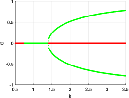
(a)

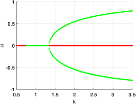
(b)

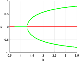
(c)

Figure 1: The spontaneous symmetry breaking of patterns supported by the double-peak spatial modulation of the nonlinearity. Asymmetry parameter (11) is displayed vs. propagation constant $k$, as obtained from the numerical solution of Eq. (3) with $\alpha=0.5$, $\beta=0$, and $g(x)$ taken as per the second line in Table 1 with $\Delta=0.244$. The three panels correspond to different strengths of the background nonlinearity: $\sigma=-1$ (a), $\sigma=0$ (b), and $\sigma=+1$ (c). Green and red branches represent stable and unstable solutions, respectively. Red segments of the symmetric solutions ($\Theta=0$) at small $k$ correspond to very weak(actually, formal) instability of modes with the convex shape, see below.

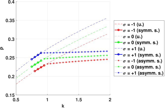
(a)

Figure 2: The total power as a function of the propagation constant, $k$, for families of symmetric and asymmetric states in the system with the double-peak singular modulation of the local nonlinearity, for $\Delta=0.293$ in the second line of Table 1, $\alpha=0.5$, $\beta=0$ and different values of $\sigma$ in Eq. (3). Here, and in Fig. 6a below, symbols in the notation box mean: “u.” - unstable symmetric solutions, “symm. s.” - stable symmetric ones, and “asymm. s.” - stable asymmetric states.

Generic examples of stationary symmetric and asymmetric modes are displayed in Figs. 3(c) and 3(a), respectively. The conclusion about the destabilization of the symmetric states at the SSB point, which was produced by the calculation of stability eigenvalues by means of Eq. (9), is confirmed by direct simulations, demonstrating that unstable symmetric states spontaneously transform into their stable asymmetric counterparts, as shown in Fig. 4.

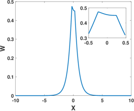
(a)

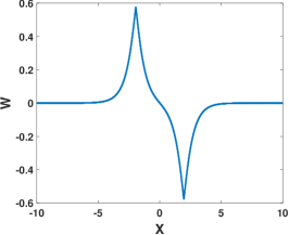
(b)

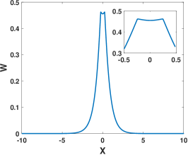
(c)

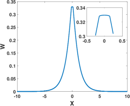
(d)

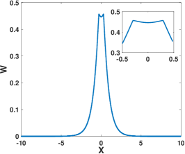
(e)

Figure 3: Typical shapes of modes pinned to the double-peak nonlinearity-modulation pattern. Panels (a), (b), and (c) display, respectively, a stable weakly asymmetric state with $\Theta=0.0525$, an unstable twisted (antisymmetric) one, and an unstable symmetric state, for $\Delta=0.244$, and a fixed value of the propagation constant, $k=1.4$. (d) An example of a formally (very weakly) unstable symmetric state with the convex shape, for $\Delta=0.1465$ and $k=0.55$. (e) A completely stable symmetric state with the concave shape, for the $\Delta=0.293$ and $k=1.3$. Insets in (d) and (e) zoom the convex and concave top parts of the respective profiles. In all the panels, other parameters in Eq. (3) are $\alpha=0.5,$ $\sigma=-1,$ and $\beta=0$.

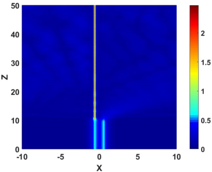
(a)

Figure 4: The spontaneous transformation of an unstable symmetric state into a stable asymmetric one in the double-peak system, for $\alpha=0.5$, $\sigma=-1$, $\Delta=0.586$, and $k=2$.

Data concerning the location of the SSB (i.e., bifurcation) points are collected in Fig. 5, which provides a comprehensive map of the parameter space of the double-peak setting. It is seen that, as mentioned above, the dependence of the critical values of the propagation constant ($k$) and total power ($P$) on the strength of the background nonlinearity, $\sigma$, is quite weak, while the dependence on the modulation’s singularity degree, $\alpha$ [see Table 1], is essential. Naturally, $k\rightarrow\infty$ and $P\rightarrow\infty$ is observed Fig. 5 at $\Delta\rightarrow 0$, as the SSB may happen if the width of the mode pinned to an individual peak, which scales as $k^{-1/2}$, has the same order of magnitude as $\Delta$.

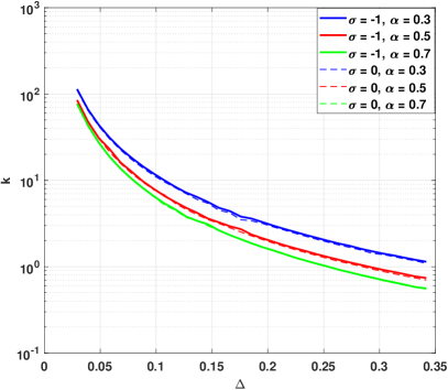
(a)

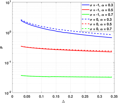
(b)

Figure 5: Values of the propagation constant, $k$ (a), and total power, $P$ (b), at the point of the spontaneous-symmetry-breaking bifurcation, vs. half-separation, $\Delta$, between the two nonlinearity-modulation peaks, with $\beta=0$. The dependences are shown on the log scale, for different values of the singular-modulation power, $\alpha$, and background-nonlinearity strength, $\sigma$.

Unlike the uniform background nonlinearity, the presence of the linear component of the modulation peaks, represented by coefficient $\beta$ in Eq. (2), produces a strong effect on the SSB scenario. Namely, $\beta>0$ (which correspond to the repulsive linear potential) leads to partial destabilization of the asymmetric states, as shown in Fig. 6a. In this case, the pair of the singular-modulation peaks may support two different asymmetric states: one with a relatively small difference between amplitudes of the solution at the two peaks, and a fully asymmetric state, strongly pinned to one of the peaks. The repulsive linear potential destabilizes the weakly asymmetric state, converting it into an asymmetric breather, as shown in Fig. 7(a). On the other hand, the unstable symmetric states are transformed into strongly asymmetric modes pinned to one of the peaks, as shown in Fig. 7(b). This finding may be explained by the fact that the increase of the amplitude of the pinned soliton helps the nonlinear attractive potential to overcome the repulsion induced by the linear potential. On the other hand, symmetric states, unlike the asymmetric ones, are not destabilized by the linear component of the modulation peaks.

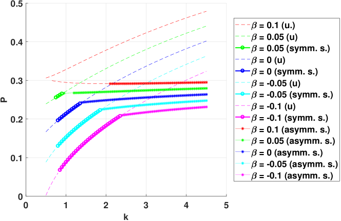
(a)

Figure 6: The same as in Fig. 2, but for $\alpha=0.5$, $\sigma=-1$, $\Delta=0.244$, and different values of $\beta$. It is seen that, in the presence of $\beta>0$, weakly asymmetric stationary states become partially unstable (see, e.g., the solution families for $\beta=0.05$, where a gap between chains of green circles and stars corresponds to the instability). The instability leads to transformation of the weakly asymmetric modes into asymmetric breathers, as shown in Fig. 7(a)

.

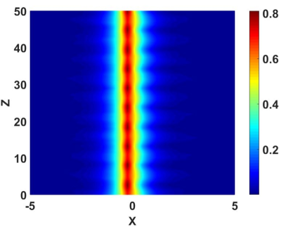
(a)

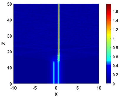
(b)

Figure 7: The development of the instability of (a) unstable asymmetric state with $\Theta=0.4043$ for $\alpha=0.5$, $\Delta=0.2441$, $\sigma=-1$, and $k=1.2$ in the presence of the repulsive linear-potential component in the singular-modulation double peak, corresponding to $\beta=0.1$ and (b) an unstable symmetric state, for $\alpha=0.5$, $\Delta=0.586$, $\sigma=-1$, and $k=2$, in the presence of the repulsive linear-potential component corresponding to $\beta=-0.1$.

In the limit case when the localized modes pinned to adjacent nonlinearity peaks are strongly overlapped, the two modes merge into a nearly flat-top one, with the small deviation of the flatness corresponding to slightly convex or concave shapes, as shown in Figs. 3(d) and 3(e), respectively. Further analysis demonstrates that the concave shapes are completely stable, while the computation of the eigenvalues of operator (9) for convex ones (which appear when the two individual modes become completely overlapping) features a very weak instability, that corresponds to short red segments near the left edge of all the panels in Fig. 1. The eigenvalues that characterize the instability are limited to be $\lesssim 10^{-4}$. Actually, direct simulations do not reveal any tangible instability of the convex profiles, in accordance with the fact that the corresponding eigenvalues are extremely small. Boundaries between the nearly flat-top convex and concave profiles in the plane of $\left(k,\Delta\right)$ for different values of $\alpha$ are displayed in Fig. 8. It is also relevant to mention that, in accordance with the results of [34], where it was demonstrated that modes pinned to a single modulation peak, competing with the self-defocusing uniform background ($\sigma=+1$), exist if their total power exceeds a certain threshold (minimum) value, the same effect was found here for the symmetric modes, the threshold being virtually exactly equal to twice the one found in [34] (this feature is not shown in detail here).

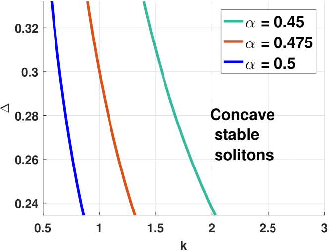
(a)

Figure 8: Boundaries between areas occupied by strongly overlapped modes with concave (completely stable) shapes, and concave ones, subject to a very weak instability. Here, $\sigma=-1$ and $\beta=0$ are fixed, the boundaries being shown for three different values of $\alpha$, as indicated in the figure.

Lastly, the model with two singular-modulation peaks admits solutions for antisymmetric (twisted) pinned modes too. However, both the computation of the stability eigenvalues and direct simulations reveal that all the twisted states are unstable. As shown in Fig. 9, the instability transforms them into robust breathers, which preserve the twisted structure.

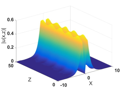
(a)

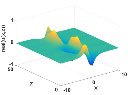
(b)

Figure 9: The evolution of an antisymmetric (twisted) mode, for $\alpha=0.5$, $\sigma=-1$, $\Delta=0.9766$, $\beta=0$, and $k=0.55$. (a) The plot of $\left|u\left(x,z\right)\right|$ displays the spontaneous transformation of the unstable twisted model into a breather. (b) The plot of the real part of $u(x,z)$ demonstrates that the breather keeps the original antisymmetric structure.

3.1 The system with three and five singular-modulation peaks

The transition from the double singular-modulation peaks to a triple one (which corresponds to the third line in Table 1) is of obvious interest, as it makes it possible to understand respective changes in the variety of pinned modes with different symmetries. In this case, asymmetric modes (stable or unstable ones) have not been found, while symmetric states exist in two varieties, viz., with in-phase and out-of-phase (alias twisted) shapes, which are shown in Fig. 10. The computation of the corresponding eigenvalues, as well as direct simulations, demonstrates that the in-phase modes with $k=1.2$ have their stability regions at $\Delta<0.66$ and $\Delta<0.61$ for $\sigma=+1$ and $-1$, respectively, as shown in Fig. 11(a) (the stability regions have similar shapes at other values of $k$). In this region, the modes are strongly overlapped, seeming as a single local-power peak, see Fig. 11(b).

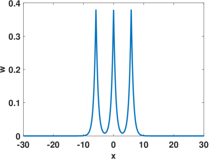
(a)

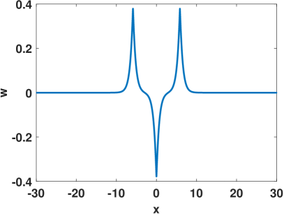
(b)

Figure 10: Modes pinned to the set of three singular-modulation peaks, which corresponds to the third line in Table 1, with $\Delta=5.86$, and $\sigma=-1$, $\beta=0$ in Eq. (2). (a) An unstable in-phase mode, with well-separated peaks [cf. the overlapped in-phase mode in Fig. 11(b)]. (b) A stable twisted mode. Both modes were obtained for propagation constant $k=1.2$.

Outside of the above-mentioned regions, the in-phase states are always unstable (unless separation $\Delta$ between the peaks is so large in comparison to the width of local modes pinned to individual peaks that they practically do not interact), while twisted modes have a nontrivial stability area in the parameter plane of $\left(\Delta,\alpha\right)$, as shown in Fig. 12. It is worthy to note a conspicuous dependence of the stability boundaries on strength $\sigma$ of the uniform nonlinearity background in Figs. 11 and 12, unlike a much weaker dependence on $\sigma$ in the case of the double peak, cf. Fig. 5.

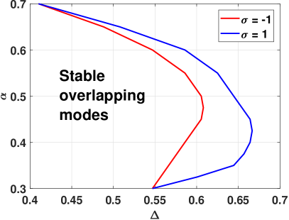
(a)

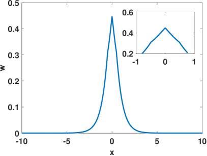
(b)

Figure 11: (a) Stability regions for strongly overlapping in-phase symmetric modes pinned by the triple singular-modulation peak, in the plane of $\left(\Delta,\alpha\right)$ for $\sigma=\pm 1$, while other parameters are $\beta=0$ and $k=1.2$. (b) A typical example of the stable mode, found at $\Delta=0.4883$ and $\alpha=0.5$. The inset zooms the shape of the mode in the region where it covers the three singularity peaks.

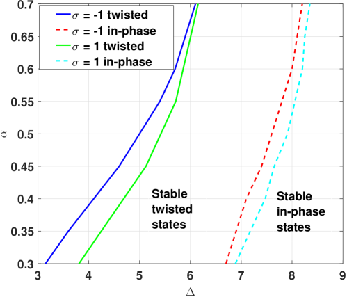
(a)

Figure 12: Stability boundaries for twisted modes pinned to the set of three peaks in the plane of $\left(\Delta,\alpha\right)$, represented by the third line in Table 1 (the twisted modes are unstable on the left-hand side of the continuous boundary lines). In this figure, $\beta=0$ and $k=1.2$ are fixed, while the strength of the background uniform nonlinearity $\sigma$ takes both values $\sigma=+1$ and $-1$ (the self-defocusing and focusing background, respectively). Beyond the dashed boundaries, in-phase modes cease being unstable because the interaction between different modes pinned to individual peaks becomes negligible.

In direct simulations, all unstable modes pinned to the triple peak spontaneously transform into patterns featuring either a state pinned to the central peak, while the edge modes disappear, or two narrow modes pinned to the edge peaks, while the central one disappears, see examples in Fig. 13. In the latter case, the emerging pattern seems to be stable because the narrow modes of which it is built virtually do not interact with each other.

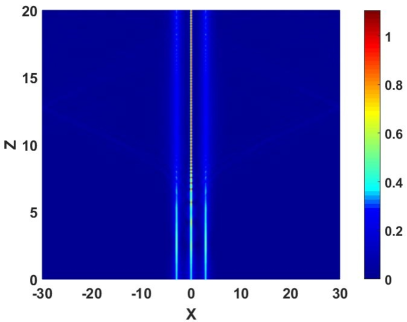
(a)

(b)

Figure 13: Spontaneous transformation of an unstable in-phase state pinned to a triple peak, corresponding to the third line in Table 1, with $\alpha=0.5$, $\sigma=-1$, $\beta=0$, propagation constant $k=1.2$ and (a) $\Delta=2.93$, or (b) $\Delta=2.34$.

As mentioned above, the consideration of the set of five modulation peaks, which corresponds to the fourth line in Table 1, is relevant too, as it is a prototype of a periodic lattice of nonlinear defects [7]. In this case, no states with broken symmetry could be produced, similar to the above-mentioned situation with the triple peak. As concerns symmetric states, all of them, of both in-phase and twisted types (see examples in Fig. 14), have been found to be unstable, i.e., the nonlinear lattice of the singular-modulation peaks, unlike the double and triple peaks, is not able to support stable states which attach local modes to all the peaks [unless separation $\Delta$ between adjacent ones is so large in comparison with widths of the modes pinned to individual peaks that they cease to interact, or so small that a single narrow mode can cover all of them, cf. Fig. 11(b)]. In direct simulations (not shown here in detail), unstable states supported by the five-peak set transform themselves into “rarefied” patterns formed by three narrow modes pinned to the central peak and two edge ones, while intermediate peaks (the second and fourth ones) remain empty, quite similar to what is shown in Fig. 13 for unstable states in the case of the triple peak. The emergent pattern seems stable because individual pinned modes do not interact. This instability and its development scenario resemble the modulational instability of extended states pinned to periodic potentials in the NLS equation with the self-attractive nonlinearity [48, 49, 7].

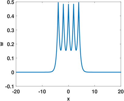
(a)

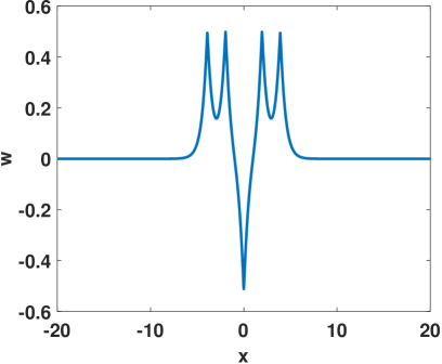
(b)

Figure 14: Examples of (a) fully in-phase and (b) combined in-phase-twisted unstable states attached to the set of five singular-nonlinearity-modulation peaks, which corresponds to the fourth line in Table 1. The parameters are: $\sigma=-1$, $\alpha=0.5$, $\Delta=1.95$, $k=2$ and $\beta=0$.

3.2 Collisions of free solitons with the nonlinearity-modulation peak

Equation Eq. (2) with the self-focusing uniform nonlinearity ($\sigma=-1$) obviously supports free NLS solitons far from the location of the peaks:

$$u_{\mathrm{sol}}\left(x,z\right)=\frac{P}{2}\exp\left[ivx+\frac{i}{2}\left(\frac{P^{2}}{4}-v^{2}\right)z\right]\mathrm{sech}\left(\frac{P}{2}\left(x-vz\right)\right),$$ (12)

where $P$ is the soliton’s total power, and $v$ is its velocity [in terms of the spatial optical solitons, it is the tilt of beam in the $\left(x,z\right)$ plane]. In this case, it is natural to consider collisions of freely moving solitons with peaks. Here, we limit the consideration to the basic case of the collision with a single peak, as this case was not studied previously either.

An essential result of systematic simulations is that, in most cases, the incident soliton bounces back from the singular-modulation peak if its velocity (tilt) is smaller than a certain critical value, $v<v_{\mathrm{cr}}$. The soliton is destroyed by the collision into a radiation wave train at $v\simeq v_{\mathrm{cr}}$, and, finally, the collision is quasi-elastic at $v\gg$ $v_{\mathrm{cr}}$, see typical examples in Figs. 15. The dependence of the trapped, reflected, and transferred shares of the total power on the incidence velocity is shown in Fig. 16. The dependence of $v_{\mathrm{cr}}$ on power $P$ of the impinging soliton for different values of the singular-modulation power $\alpha$ is shown in Fig. 17.

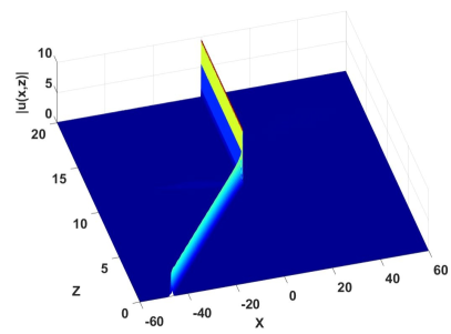
(a)

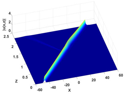
(b)

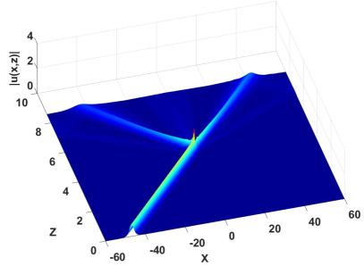
(c)

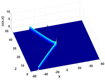
(d)

Figure 15: Collisions of an incident free soliton (12) with the nonlinearity-modulation peak, corresponding to the first line in Table 1 with $\sigma=-1$ and $\beta=0$. (a) The special case of resonant trapping of the incident soliton with $P=8$ at $\alpha=0.6$ and $v=4.5$. (b) Elastic collision of the incident soliton, with $P=3$ and $v=40$, impinging on the nonlinearity peak with the singular-modulation power $\alpha=0.3$. (c) Nearly complete destruction of the incident soliton with $P=2$ at the critical velocity, $v_{\mathrm{cr}}=10.5$, for $\alpha=0.5$. (d) The rebound of the soliton with $P=5$ from the peak with the singular-modulation power $\alpha=0.6$ at a small incidence velocity (tilt), $v=2$.

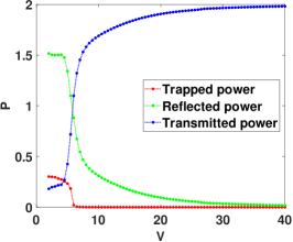
(a)

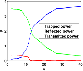
(b)

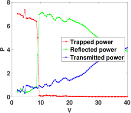
(c)

Figure 16: Shares of the total power of the incident free soliton with (a) $P_{\mathrm{sol}}=2$, which corresponds to the propagation constant $k=0.5$ of the free soliton with zero velocity (tilt) and (b) $P_{\mathrm{sol}}=4$, which corresponds to propagation constant $k=2$ of the free soliton with zero velocity (tilt), that are trapped (the red curve) , reflected (the green curve) and keep the original direction of the motion (“transmitted power”, depicted by the blue curve), versus the incidence velocity, $v$. The solitons impinge on the nonlinearity peak with $\sigma=-1$, $\beta=0$, and $\alpha=0.4$. The respective critical velocity, at which the soliton is completely destroyed by the collision is $v_{\mathrm{cr}}\approx 6$ for the soliton with $P_{\mathrm{sol}}=2$, and $v_{\mathrm{cr}}\approx 13$ for the one with $P_{\mathrm{sol}}=4$. Panel (c) illustrates the special case of the resonant capture of the incident soliton, an example of which is displayed in Fig. 15(a). In this case, the parameters are $\sigma=-1$, $\beta=0$, $\alpha=0.6$, and $P_{\mathrm{sol}}=8$.

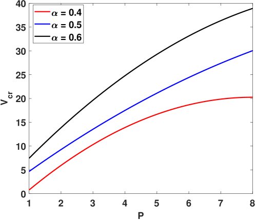
(a)

Figure 17: $v_{\mathrm{cr}}$ as a function of power $P$ of the moving soliton, and singular-modulation parameter $\alpha$, at $\sigma=-1$ and $\beta=0$.

The fact that the incident soliton readily bounces back from the singular-modulation peak, which represents an attractive nonlinear defect, is remarkable by itself, as rebound is normally expected from repulsive defects. Previously, rebound of solitons impinging on an (attractive) linear potential well was reported in [50, 51].

Capture of the incident soliton by the peak was observed too, but only under a specific condition, which may be considered as a resonant one: a soliton with total power $P$ gets captured, as shown in Fig. 15(a), if its propagation constant in the quiescent state, i.e., $k_{\mathrm{sol}}(v=0)=P^{2}/8$, see Eq. (12), is close to the value of $k$ for the mode with the same value of $P$ trapped by the self-focusing peak, while the velocity of the incoming soliton is relatively small. This special case is illustrated by dependences of the of the trapped, reflected, and transferred shares of the total power on $v$ shown in Fig. 16(c). The resonant situation can be approximately predicted by equating $k_{\mathrm{sol}}(v=0)$ to the propagation constant predicted, for the same value of $P$, by the VA, i.e., by the Euler-Lagrange equations following from the effective Lagrangian (7) (not shown here in detail).

4 Conclusions

We have introduced the 1D model with the cubic self-focusing nonlinearity locally modulated by a set of singular profiles, while the background uniform nonlinearity may be focusing or defocusing. The possibility of the modulation peaks including the linear-potential components is considered too. Numerical analysis has demonstrated that the setting with a pair of symmetric peaks readily gives rise to the SSB (spontaneous symmetry breaking) of the modes pinned to the individual peaks, via the supercritical bifurcation. The antisymmetric states were found too, turning out to be unstable and transforming into antisymmetric breathers. Sets of three and five peaks do not give rise to asymmetric states, rather supporting symmetric ones, with in-phase or twisted profiles. The twisted states pinned to the triple peaks have their stability area, while the in-phase modes are unstable, except for the strongly overlapping ones. The sets of five peaks fails to support any stable nontrivial modes.

References

- [1] V. E. Zakharov, S. V. Manakov, S. P. Novikov, and L. P. Pitaevskii, Solitons: the Inverse Scattering Transform Method (Nauka Publishers, Moscow, 1980 (in Russian); English translation: Consultants Bureau, New York, 1984).
- [2] M. Ablowitz and H. Segur, Solitons and the Inverse Scattering Transform (SIAM, Philadelphia, 1981); A. C. Newell, Solitons in Mathematics and Physics (SIAM, Philadelphia, 1985).
- [3] Y. S. Kivshar and G. P. Agrawal, Optical Solitons: From Fibers in Photonic Crystals (Academic Press: San Diego, 2003); T. Dauxois and M. Peyrard, Physics of Solitons (Cambridge University, Cambridge, 2006).
- [4] B. A. Malomed, D. Mihalache, F. Wise, and L. Torner, Spatiotemporal optical solitons, J. Optics B: Quant. Semicl. Opt. 7, R53 (2005); Viewpoint: On multidimensional solitons and their legacy in contemporary Atomic, Molecular and Optical physics, J. Phys. B: At. Mol. Opt. Phys. 49, 170502 (2016).
- [5] J. Yang, Nonlinear Waves in Integrable and Nonintegrable Systems (SIAM: Philadelphia, 2010).
- [6] J. Satsuma and N. Yajima, B. Initial Value Problems of One-Dimensional Self-Modulation of Nonlinear Waves in Dispersive Media, Suppl. Prog. Theor. Phys. No. 55, p. 284-306 (1974).
- [7] Y. V. Kartashov, B. A. Malomed, and L. Torner, Solitons in nonlinear lattices, Rev. Mod. Phys. 83, 247 (2011).
- [8] J. Hukriede, J., D. Runde, and D. Kip, Fabrication and application of holographic Bragg gratings in lithium niobate channel waveguides, J. Phys. D 36, R1 (2003).
- [9] Y. Kominis, Analytical solitary wave solutions of the nonlinear Kronig-Penney model in photonic structures, Phys. Rev. E 73, 066619 (2006).
- [10] Y. Kominis, and K. Hizanidis, Lattice solitons in self-defocusing optical media: analytical solutions of the nonlinear Kronig-Penney model, Opt. Lett. 31, 2888-2890 (2006).
- [11] Power dependent soliton location and stability in complex photonic structures, Opt. Express 16, 12124-12138 (2008).
- [12] Y. Kominis, Bright, dark, antidark, and kink solitons in media with periodically alternating sign of nonlinearity Phys. Rev. A 87, 063849 (2013).
- [13] P. O. Fedichev, Y. Kagan, G. V. Shlyapnikov, and J. T. M. Walraven, Influence of Nearly Resonant Light on the Scattering Length in Low-Temperature Atomic Gases, Phys. Rev. Lett. 77, 2913-2916 (1996).
- [14] M. Theis, G. Thalhammer, K. Winkler, M. Hellwig, G. Ruff, R. Grimm, and J. H. Denschlag, Tuning the Scattering Length with an Optically Induced Feshbach Resonance, Phys. Rev. Lett. 93, 123001 (2004).
- [15] M. Yan, B. J. DeSalvo, B. Ramachandhran, H. Pu, and T. C. Killian, Controlling Condensate Collapse and Expansion with an Optical Feshbach Resonance, Phys. Rev. Lett. 110, 123201 (2013).
- [16] K. Henderson, C. Ryu, C. MacCormick, and M. G. I. Boshier, Experimental demonstration of painting arbitrary and dynamic potentials for Bose-Einstein condensates, New J. Phys. 11, 043030 (2009).
- [17] C. Ryu, P. W. Blackburn, A. A. Blinova, and M. G. Boshier, Experimental Realization of Josephson Junctions for an Atom SQUID, Phys. Rev. Lett. 111, 205301 (2013).
- [18] H. S. Ghanbari, T. D. Kieu, A. Sidorov, and P. Hannaford, Permanent magnetic lattices for ultracold atoms and quantum degenerate gases, J. Phys. B: At. Mol. Opt. Phys. 39, 847 (2006).
- [19] O. Romero-Isart, C. Navau, A. Sanchez, P. Zoller, and J. I. Cirac, Superconducting Vortex Lattices for Ultracold Atoms, Phys. Rev. Lett. 111, 145304 (2013).
- [20] S. Ghanbari, A. Abdalrahman, A. Sidorov, and P. Hannaford, Analysis of a simple square magnetic lattice for ultracold atoms, J. Phys. B: At. Mol. Opt. Phys. 47, 115301 (2014).
- [21] B. A. Malomed and M. Y. Azbel, Modulational instability of a wave scattered by a nonlinear center, Phys. Rev. B 47, 10402-10406 (1993).
- [22] T. Mayteevarunyoo, B. A. Malomed, and G. Dong, Spontaneous symmetry breaking in a nonlinear double-well structure, Phys. Rev. A 78, 053601 (2008).
- [23] N. Dror and B. A. Malomed, Solitons supported by localized nonlinearities in periodic media, Phys. Rev. A 83, 033828 (2011).
- [24] A. Acus, B. A. Malomed, and Y. Shnir, Spontaneous symmetry breaking of binary fields in a nonlinear double-well structure, Physica D 241, 987-1002 (2012).
- [25] H. Sakaguchi and B. A. Malomed, Matter-wave soliton interferometer based on a nonlinear splitter, New J. Phys. 18, 025020 (2016).
- [26] M. I. Molina and G. P. Tsironis, Nonlinear impurities in a linear chain, Phys. Rev. B 47, 15330-15333 (1993).
- [27] B. Maes, M. Soljačić, J. D. Joannopoulos, P. Bienstman, R. Baets, S.-P. Gorza, and M. Haelterman, Switching through symmetry breaking in coupled nonlinear micro-cavities, Opt. Exp. 14, 10678-10683(2006)
- [28] E. N. Bulgakov and A. F. Sadreev, Bound states in photonic Fabry-Perot resonator with nonlinear off-channel defects, Phys. Rev. B 81, 115128 (2010).
- [29] V. A. Brazhnyi and B. A. Malomed, Spontaneous symmetry breaking in Schrödinger lattices with two nonlinear sites, Phys. Rev. A 83, 053844 (2011).
- [30] E. A. Kuznetsov and F. Dias, Bifurcations of solitons and their stability, Phys. Rep. 507, 43 (2011).
- [31] L. Bergé, Wave collapse in physics: Principles and applications to light and plasma waves, Phys. Rep. 303, 259 (1998).
- [32] G. Fibich, The Nonlinear Schrödinger Equation: Singular Solutions and Optical Collapse, (Springer: Heidelberg, 2015).
- [33] Yu. B. Gaididei, J. Schjodt-Eriksen, and P. L. Christiansen, Collapse arresting in an inhomogeneous quintic nonlinear Schrödinger model, Phys. Rev. E 60, 4877 (1999); F. Kh. Abdullaev and M. Salerno, Gap-Townes solitons and localized excitations in low-dimensional Bose-Einstein condensates in optical lattices, Phys. Rev. A 72, 033617 (2005).
- [34] O. V. Borovkova, V. E. Lobanov, and B. A. Malomed, Solitons supported by singular spatial modulation of the Kerr nonlinearity, Phys. Rev. A 85, 023845 (2012).
- [35] Spontaneous Symmetry Breaking, Self-Trapping, and Josephson Oscillations, Editor: B. A. Malomed (Springer-Verlag: Berlin and Heidelberg, 2013).
- [36] A. A. Sukhorukov and Y. S. Kivshar, Nonlinear localized waves in a periodic medium, Phys. Rev. Lett. 87, 083901 (2001).
- [37] A. A. Sukhorukov and Y. S. Kivshar, Spatial optical solitons in nonlinear photonic crystals, Phys. Rev. E 65, 036609 (2002).
- [38] A. Shapira, N. Voloch-Bloch, B. A. Malomed, and A. Arie, Spatial quadratic solitons guided by narrow layers of a nonlinear material, J. Opt. Soc. Am. B 28, 1481-1489 (2011).
- [39] I. L. Garanovich, S. Longhi, A. A. Sukhorukov, and Y. S. Kivshar, Light propagation and localization in modulated photonic lattices and waveguides, Phys. Rep. 518, 1 (2012).
- [40] A. B. Aceves, J. V. Moloney, and A. C. Newell, Theory of light-beam propagation at nonlinear interfaces. I. Equivalent-particle theory for a single interface, Phys. Rev. A 39, 1809 (1989).
- [41] A. B. Aceves, J. V. Moloney, and A. C. Newell, Theory of light-beam propagation at nonlinear interfaces. II. Multiple-particle and multiple-interface extensions, Phys. Rev. A 39, 1828 (1989).
- [42] W. C. K. Mak, B. A. Malomed, and P. L. Chu. Interaction of a soliton with a local defect in a fiber Bragg grating. J. Opt. Soc. Am. B 20, 725-735 (2003).
- [43] R. H. Goodman, P. J. Holmes, M. I. Weinstein, Strong NLS soliton-defect interactions, Physica D 192 215 (2004).
- [44] M. T. Primatarowa, K. T. Stoychev, and R. S. Kamburova, Interaction of solitons with extended nonlinear defects, Phys. Rev. E 72, 036608 (2005).
- [45] J. Garnier and F. Kh. Abdullaev, Transmission of matter-wave solitons through nonlinear traps and barriers, Phys. Rev. A 74, 013604 (2006).
- [46] Y. Kominis and K. Hizanidis, Power-Dependent Reflection, Transmission, and Trapping Dynamics of Lattice Solitons at Interfaces, Phys. Rev Lett. 102, 133903 (2009).
- [47] G. Iooss and D. D. Joseph, Elementary Stability and Bifurcation Theory, (Springer: New York, 1980).
- [48] M. Centurion, M. A. Porter, Y. Pu, P. G. Kevrekidis, D. J. Frantzeskakis, and D. Psaltis, Modulational Instability in a Layered Kerr Medium: Theory and Experiment, Phys. Rev. Lett. 97, 234101 (2006).
- [49] F. Kh. Abdullaev, Yu. V. Bludov, S. V. Dmitriev, P. G. Kevrekidis, and V. V. Konotop, Generalized neighbor-interaction models induced by nonlinear lattices, Phys. Rev. E 77, 016604 (2008).
- [50] C. Lee and J. Brand, Enhanced quantum reflection of matter-wave solitons, Europhys. Lett. 73, 321 (2006).
- [51] T. Ernst and J. Brand, Resonant trapping in the transport of a matter-wave soliton through a quantum well, Phys. Rev. A 81, 033614 (2010).