Semiclassical approximation to the Hartree-Fock method in finite nuclei

Abstract

In this paper we review the semiclassical extended Thomas–Fermi theory for describing the ground-state properties of nuclei. The binding energies calculated in this approach do not contain shell effects and, in this sense, they are analogous to those obtained from the mass formula. We discuss some techniques for incorporating the shell effects which are missing in the semiclassical calculation, such as the so-called expectation value method and the Kohn-Sham scheme. We present numerical applications for effective zero-range Skyrme forces and finite-range Gogny forces.

1 Introduction

To obtain the ground-state energy and the particle density of a set of interacting nucleons is one of the most important problems in nuclear physics. This is a complicated many-body problem if realistic nucleon-nucleon interactions are used. To overcome the difficulties effective nucleon-nucleon forces and approximated schemes have been proposed. One of the most outstanding approaches is the Hartree–Fock (HF) method, which consists in replacing the many-body wave function by a Slater determinant of single-particle wave functions. These wave functions are obtained self-consistently from the mean field produced by the nucleons.

When used together with effective density-dependent nucleon-nucleon forces, like for example the Skyrme [1], Gogny [2] or M3Y [3] interactions, the HF method is a very powerful tool to carry out in a simple way accurate nuclear structure calculations. This density-dependent HF (DDHF) approach yields binding energies and root-mean square radii in very good agreement with experiment. These simple forces are also able to describe dynamical phenomena such as excited nuclei properties, nuclear excitation spectra, nucleon-nucleus optical potential and low energy heavy-ion scattering (see for example [4] for a review for Skyrme forces).

Another different approach within the mean field theory is the so-called density functional theory (DFT). The basic idea of DFT is that the ground-state energy of a system of interacting fermions can be expressed by an integral over the whole space of an energy density which depends only on the ground-state local density $\rho(\mbox{\boldmath$R$})$:

$$E[\rho]=\int\varepsilon[\rho]d\mbox{\boldmath$R$}.$$ (1)

The theoretical justification of DFT is provided by the Hohenberg–Kohn theorem [5]. It states that the exact non-degenerate ground-state energy of a correlated electron system is a functional of the local density $\rho(\mbox{\boldmath$R$})$ and that this functional has its variational minimum when evaluated with the exact ground-state density:

$$\frac{\delta}{\delta\rho}\bigg{[}E[\rho]-\mu\int\rho(\mbox{\boldmath$R$})d\mbox{\boldmath$R$}\bigg{]}=0,$$ (2)

where $\mu$ is the Lagrange multiplier for ensuring the right number of particles.

Unfortunately, $\varepsilon[\rho]$ is not exactly known for a finite interacting fermion system and consequently approximations are in order. It is useful to break up the energy of the system in several pieces by writing

$$E[\rho]=T[\rho]+\frac{1}{2}\int V_{H}[\rho]\rho(\mbox{\boldmath$R$})d\mbox{\boldmath$R$}+E_{ex}[\rho],$$ (3)

where $T[\rho]$ is the kinetic energy of a system of non-interacting fermions of density $\rho$ and $V_{H}[\rho]$ is the direct (Hartree) potential given by

$$V_{H}[\rho]=\int v(\mbox{\boldmath$R$},\mbox{\boldmath$R^{\prime}$})\rho(\mbox{\boldmath$R^{\prime}$})d\mbox{\boldmath$R^{\prime}$},$$ (4)

with $v(\mbox{\boldmath$R$},\mbox{\boldmath$R^{\prime}$})$ the effective nucleon-nucleon interaction. The last term in eq. (3) is the so-called exchange-correlation energy that contains the exchange energy as well as contributions of the correlations due to the fact that the exact wave function is not a Slater determinant.

The kinetic energy functional $T[\rho]$ is not known exactly either. Kohn and Sham (KS) [6] proposed to write the local density in terms of trial single-particle wave functions $\phi_{i}(\mbox{\boldmath$R$})$ as

$$\rho(\mbox{\boldmath$R$})=\sum^{A}_{i=1}{|\phi_{i}(\mbox{\boldmath$R$})|}^{2},$$ (5)

furthermore assuming that the kinetic energy density functional can also be expressed through the same trial single-particle wave functions:

$$\frac{\hbar^{2}}{2m}\tau(\mbox{\boldmath$R$})=\frac{\hbar^{2}}{2m}\sum^{A}_{i=1}{|\mbox{\boldmath$\nabla$}\phi_{i}(\mbox{\boldmath$R$})|}^{2}.$$ (6)

With the help of eqs. (5)-(6), the variation with respect to $\rho$ in eq. (2) can be easily carried out to obtain

$$\big{\{}-\frac{\hbar^{2}}{2m}\Delta+V_{H}(\mbox{\boldmath$R$})+\frac{\delta E_{ex}}{\delta\rho}\big{\}}\phi_{i}(\mbox{\boldmath$R$})=\varepsilon_{i}\phi_{i}(\mbox{\boldmath$R$}),$$ (7)

which are known as Kohn–Sham equations. These equations are similar to the HF ones, although the KS potential

$$V_{KS}(\mbox{\boldmath$R$})=V_{H}(\mbox{\boldmath$R$})+\frac{\delta E_{ex}}{\delta\rho}$$ (8)

is local as compared with the, in general, non-local HF potential. The difference between the exact kinetic energy density functional and the approximated functional given by eq. (6) is included in the exchange-correlation term $E_{ex}$.

Although the KS approach is exact if one deals with the exact $E_{ex}$, this theory is not free of certain difficulties. First, the physical interpretation of the KS orbitals is not clear. In view of eq. (7) they are often considered as a HF wave function. However, there is no real justification for it because no assumption is done about representing the many-body wave function by a Slater determinant. On the other hand, the physical meaning of the eigenvalues $\varepsilon_{i}$ of eq. (7) is not clear either because the Koopmans’ theorem, valid in the HF approach, does not apply in the KS scheme. It should also be pointed out that the kinetic energy density, eq. (6), is only an approach to the exact one because the existence of a set of single-particle wave functions obeying simultaneously eqs. (5) and (6) has not been proved [7].

Alternatively, another approximation consists in writing the kinetic energy density functional explicitly in terms of the local density and its gradients. In such a case the variational equation (2) allows one to find $\rho(\mbox{\boldmath$R$})$ directly, avoiding the task of solving the KS equations. The simplest case is just the Thomas-Fermi (TF) approximation, where the kinetic energy density is written as

$$T[\rho]=\frac{\hbar^{2}}{2m}\frac{3}{5}({\frac{3\pi^{2}}{2}})^{2/3}\rho^{5/3},$$ (9)

if a degeneracy 4 is assumed.

The TF approach is exact at the quantal level for an uniform system and therefore does not contain shell effects. When applied to finite nuclei, it implies that in the neighbourhood of a point $R$ the nucleus behaves as a piece of nuclear matter of density $\rho(\mbox{\boldmath$R$})$. Thus, for a finite nucleus the TF energy represents an average energy and it is similar in spirit to the one obtained with the mass formula derived within the liquid drop or droplet models [8]. The success of these semiclassical approaches lies on the fact that the quantal corrections (shell effects) are small as compared with the part of the energy that varies slowly with the number of particles $A$, the one which is provided by the mass formula or by the TF method.

From a theoretical point of view, the perturbative treatment of the shell correction energy in finite Fermi systems is based on the so-called Strutinsky energy theorem [9]. It states that the total quantal energy can be split in two parts:

$$E=\tilde{E}+\delta E.$$ (10)

The largest part $\tilde{E}$ varies smoothly with the number of particles $A$. It can be calculated in a way similar to the exact energy $E$, but using the smoothed density matrix (equivalent to the semiclassical one) obtained with Strutinsky averaged (SA) occupation numbers instead of the quantal density matrix [13]. The shell correction $\delta E$ has a pure quantal origin and its behaviour is not smooth at all; it is much smaller than $\tilde{E}$, although it can become important in some cases like in low-energy nuclear fission.

Brack and Quentin [11] have carried out extensive HF Strutinsky calculations with Skyrme forces. From these calculations it can be seen that the properties of $\tilde{E}$ are like those of the semiclassical liquid droplet model. They have also shown that the shell effects can be perturbatively added to the self-consistent smooth quantities. These facts suggest that it could be possible to replace the microscopic Strutinsky smooth quantities, which are rather difficult to handle in practice, by a much simpler semiclassical calculation of them.

It should be pointed out that the pure TF approximation is not well suited for the variational calculation of eq. (2). Corrections to the kinetic energy density that take into account the finite size of the nucleus have to be included, as for instance the well-known Weizsäcker correction:

$$T_{W}[\rho]=\frac{\hbar^{2}}{72m}\frac{(\mbox{\boldmath$\nabla$}{\rho})^{2}}{\rho}.$$ (11)

In a more systematic way, the extended Thomas-Fermi (ETF) method, which includes up to $\hbar^{4}$-order corrections to the kinetic energy and spin-orbit densities through the particle density and its gradients up to fourth order, has been developed in the past [12, 13]. These $\hbar^{4}$-order functionals used in conjunction with Skyrme forces, lead to fourth order and highly non-linear equations for the particle density $\rho(\mbox{\boldmath$R$})$ that can be solved self-consistently [14]. For Skyrme forces the binding energies for finite nuclei obtained including these $\hbar^{4}$-contributions are close to the Strutinsky results [13] although some differences persist due to the approximations used for obtaining the $T[\rho]$ functional in the ETF approach [15]. Very recently [16], the ETF approach has been employed to obtain the semiclassical density matrix up to $\hbar^{2}$ order in coordinate space for the case of a non-local HF potential for finite range effective nucleon-nucleon forces.

This work is devoted to the discussion of semiclassical approaches to the HF method and the comparison with full quantal results for zero-range and finite range nucleon-nucleon effective forces. The paper is organized as follows. In Section 2 we briefly present the derivation of the semiclassical ETF HF energy in the case of a finite range effective interaction. Section 3 is devoted to the study of the ETF energies using Skyrme forces with recently presented parametrizations [17] which are able to describe nuclei far from the stability line and a way for including shell effects is discussed. In Section 4 we perform ETF and KS calculations using the Gogny force. The conclusions are laid in the last Section.

2 Hartree-Fock energy in the Extended Thomas-Fermi approximation

In this section we derive the ETF HF energy for a non-local potential following closely the method presented in Refs. [15, 16]. We start from the quantal one-body Hamiltonian which for each kind of particle reads

$$\hat{H}=-\frac{\hbar^{2}}{2m}\Delta+V^{H}(\mbox{\boldmath$r$},\mbox{\boldmath$r^{\prime}$})\delta(\mbox{\boldmath$r$}-\mbox{\boldmath$r^{\prime}$})+V^{F}(\mbox{\boldmath$r$},\mbox{\boldmath$r^{\prime}$})-i\mbox{\boldmath$W$}(\mbox{\boldmath$r$},\mbox{\boldmath$r^{\prime}$})(\mbox{\boldmath$\nabla$}\times\mbox{\boldmath$\sigma$})\delta(\mbox{\boldmath$r$}-\mbox{\boldmath$r^{\prime}$}),$$ (12)

where the last term is the spin-orbit Hamiltonian. The corresponding HF energy for an uncharged nucleus can be written as

$$E_{HF} = \sum_{q}\int d\mbox{\boldmath$R$}\bigg{[}\frac{\hbar^{2}}{2m}\tau(\mbox{\boldmath$R$})+\frac{1}{2}\rho(\mbox{\boldmath$R$})V_{dir}(\mbox{\boldmath$R$})+\frac{1}{2}\int d\mbox{\boldmath$s$}V_{ex}(\mbox{\boldmath$R$},s)\rho(\mbox{\boldmath$R$}+\frac{\mbox{\boldmath$s$}}{2},\mbox{\boldmath$R$}-\frac{\mbox{\boldmath$s$}}{2})$$ (13)

$$+ \mbox{\boldmath$J$}(\mbox{\boldmath$R$})\mbox{\boldmath$W$}(\mbox{\boldmath$R$})\bigg{]}_{q},$$

where the subindex $q$ refers to each kind of nucleon. In eq. (13) $\mbox{\boldmath$R$}=(\mbox{\boldmath$r$}+\mbox{\boldmath$r^{\prime}$})/2$ and $\mbox{\boldmath$s$}=\mbox{\boldmath$r$}-\mbox{\boldmath$r^{\prime}$}$ are the center of mass and relative coordinates, and the direct ($V^{H}$) and exchange ($V^{F}$) parts of the HF potential are given by

$$V^{H}(\mbox{\boldmath$R$})=\int d\mbox{\boldmath$s$}v(\mbox{\boldmath$s$})\rho(\mbox{\boldmath$R$},\mbox{\boldmath$s$})$$ (14)

and

$$V^{F}(\mbox{\boldmath$R$})=-v(\mbox{\boldmath$s$})\rho(\mbox{\boldmath$R$}+\frac{\mbox{\boldmath$s$}}{2},\mbox{\boldmath$R$}-\frac{\mbox{\boldmath$s$}}{2}).$$ (15)

where for the sake of simplicity we use a simple Wigner force.

In terms of the one-body density matrix $\rho(\mbox{\boldmath$R$}+\frac{\mbox{\boldmath$s$}}{2},\mbox{\boldmath$R$}-\frac{\mbox{\boldmath$s$}}{2})=\sum^{A}_{i=1}\phi^{*}_{i}(\mbox{\boldmath$r$})\phi_{i}(\mbox{\boldmath$r^{\prime}$})$, the particle, kinetic energy and spin-orbit densities read

$$\rho(\mbox{\boldmath$R$})=\rho(\mbox{\boldmath$R$},\mbox{\boldmath$s$})|_{s=0}$$ (16)

$$\tau(\mbox{\boldmath$R$})=\bigg{(}\frac{1}{4}\Delta_{R}-\Delta_{s}\bigg{)}\rho(\mbox{\boldmath$R$},\mbox{\boldmath$s$})|_{s=0}$$ (17)

$$\mbox{\boldmath$J$}(\mbox{\boldmath$R$})=-i\bigg{[}\mbox{\boldmath$\sigma$}\times(\frac{1}{2}\mbox{\boldmath$\nabla$}_{R}+\mbox{\boldmath$\nabla$}_{s})\bigg{]}\rho(\mbox{\boldmath$R$},\mbox{\boldmath$s$})|_{s=0}.$$ (18)

The HF ETF energy is obtained from eq. (13) replacing the quantal densities by their corresponding ETF values. The ETF HF energy can be written as a functional of the local density only if the density matrix is expressed in terms of $\rho(\mbox{\boldmath$R$})$ and its gradients.

The simplest semiclassical approach to the density matrix corresponds to the so-called Slater or TF approximation where

$$\rho(\mbox{\boldmath$R$},s)=\frac{3j_{1}(k_{F}s)}{k_{F}s}\rho.$$ (19)

In this equation $j_{1}(k_{F}s)$ is the $l=1$ spherical Bessel function and $k_{F}$ the local Fermi momentum, which for each kind of nucleon is related with the local density by

$$k_{F}=(3\pi^{2}\rho)^{1/3}.$$ (20)

At this TF level there is no semiclassical spin-orbit contribution. On the other hand, as it has been pointed out in previous literature the Slater approach to the density matrix cannot be very accurate for describing the exchange part specially if the non-local effects are important [18, 16].

Corrections to the one-body density matrix that take into account finite-size effects have been considered in the past [18, 19]. However, we will use here the recently developed ETF approach to the one-body density matrix [16]. Usually, the semiclassical methods of TF type are based on the Wigner-Kirkwood $\hbar$ expansion of the density matrix [20]. This expansion can be obtained in several ways. The partition function approach of Bhaduri [21], the Kirzhnits expansion [22], the algebraic method of Grammaticos and Voros [12] or the direct expansion of the density matrix [23] are some examples. We will use the latter way that has been applied in the case of non-local potentials in refs. [15, 16].

The Wigner transform of the quantal single-particle Hamiltonian (12) is given by

$$H_{W}=\frac{\hbar^{2}k^{2}}{2m}+V^{H}(\mbox{\boldmath$R$})+V^{F}(\mbox{\boldmath$R$},k)-(\mbox{\boldmath$W$}(\mbox{\boldmath$R$})\times\mbox{\boldmath$k$})\mbox{\boldmath$\sigma$}=\tilde{H}_{W}+H_{so}.$$ (21)

In this equation $V^{H}(\mbox{\boldmath$R$})$ and $V^{F}(\mbox{\boldmath$R$},k)$ are the Wigner transform of the direct and exchange parts of the HF potential and are given by

$$V^{H}(\mbox{\boldmath$R$})=\int d\mbox{\boldmath$R^{\prime}$}v(\mbox{\boldmath$R$},\mbox{\boldmath$R^{\prime}$})\rho(\mbox{\boldmath$R^{\prime}$})$$ (22)

and

$$V^{F}(\mbox{\boldmath$R$},\mbox{\boldmath$k$})=g\int\frac{d\mbox{\boldmath$k^{\prime}$}}{(2\pi)^{3}}w(\mbox{\boldmath$k$},\mbox{\boldmath$k^{\prime}$})f_{W}(\mbox{\boldmath$R$},\mbox{\boldmath$k^{\prime}$}),$$ (23)

where $g$ stands for the degeneracy, $w(\mbox{\boldmath$k$},\mbox{\boldmath$k^{\prime}$})$ is the Fourier transform of the nuclear interaction $v(\mbox{\boldmath$R$},\mbox{\boldmath$R^{\prime}$})$, and $f_{W}(\mbox{\boldmath$R$},\mbox{\boldmath$k$})$ is the distribution function (Wigner transform of the density matrix).

Following ref. [15], the distribution function for a non-local potential with spherical symmetry about $k$ reads

$$\tilde{f}_{W}(\mbox{\boldmath$R$},k) = \frac{1}{4\pi}\int f_{WK}(\mbox{\boldmath$R$},\mbox{\boldmath$k$})d\Omega_{k}$$ (24)

$$= \Theta(\lambda-\tilde{H}_{W}-H_{so})-\frac{\hbar^{2}}{8m}\delta^{\prime}(\lambda-\tilde{H}_{W})F_{1}(\mbox{\boldmath$R$},k)+\frac{\hbar^{2}}{24m}\delta^{\prime\prime}(\lambda-\tilde{H}_{W})F_{2}(\mbox{\boldmath$R$},k)$$

$$= \Theta(\lambda-\tilde{H}_{W})-\frac{\hbar^{2}}{8m}\delta^{\prime}(\lambda-\tilde{H}_{W})F_{1}(\mbox{\boldmath$R$},k)+\frac{\hbar^{2}}{24m}\delta^{\prime\prime}(\lambda-\tilde{H}_{W})F_{2}(\mbox{\boldmath$R$},k)$$

$$+ \delta(\lambda-\tilde{H}_{W})(\mbox{\boldmath$W$}\times\mbox{\boldmath$k$})\sigma-\frac{1}{2}\delta^{\prime}(\lambda-\tilde{H}_{W})(\mbox{\boldmath$W$}\times\mbox{\boldmath$k$})^{2}$$

In eq. (24) the functions $F_{1}(\mbox{\boldmath$R$},k)$ and $F_{2}(\mbox{\boldmath$R$},k)$ are given by

$$F_{1}(\mbox{\boldmath$R$},k)=\frac{\hbar^{2}}{3m}\big{[}\frac{m}{\hbar^{2}}\Delta V(3f+kf_{k})-k^{2}(\mbox{\boldmath$\nabla$}{f})^{2}\big{]}$$ (25)

$$F_{2}(\mbox{\boldmath$R$},k)=\frac{\hbar^{2}}{3m}\big{[}\frac{m}{\hbar^{2}}(\mbox{\boldmath$\nabla$}{V})^{2}(3f+kf_{k})+k^{2}f^{2}\Delta V-2k^{2}f\mbox{\boldmath$\nabla$}{V}\mbox{\boldmath$\nabla$}{f}\big{]},$$ (26)

where $f$ is the inverse of the position and momentum dependent effective mass:

$$f(\mbox{\boldmath$R$},k)=\frac{m}{m^{*}(\mbox{\boldmath$R$},k)}=1+\frac{m}{\hbar^{2}k}V^{F}_{k}(\mbox{\boldmath$R$},k),$$ (27)

and the subscript $k$ indicates a partial derivative with respect to $k$. The density matrix in coordinate space is given by the inverse Wigner transform of (25):

$$\rho_{W}(\mbox{\boldmath$R$},s) = \int\frac{d\mbox{\boldmath$k$}}{(2\pi)^{3}}\tilde{f_{W}}(\mbox{\boldmath$R$},s)e^{i\mbox{\boldmath$k$}\mbox{\boldmath$s$}}$$ (28)

$$= \frac{k_{F}^{3}}{6\pi^{3}}\frac{3j_{1}(k_{F}s)}{k_{F}s}+\rho_{2,W}(\mbox{\boldmath$R$},s,k_{F}).$$

The ETF density matrix is obtained from the WK density matrix by expanding $k_{F}$ into its $\hbar^{0}$ and $\hbar^{2}$ parts and eliminating the spatial derivatives of the HF potential in favour of the local density and its gradients [15, 16]. For each kind of nucleon and after some algebra one finds

$$\tilde{\rho}(\mbox{\boldmath$R$},s) = \frac{3j_{1}(k_{F}s)}{k_{F}s}\rho+\frac{s^{2}}{216}\bigg{\{}\big{[}(9-2k_{F}\frac{f_{k}}{f}-2k_{F}^{2}\frac{f_{kk}}{f}+k_{F}^{2}\frac{f_{k}^{2}}{f^{2}})\frac{j_{1}(k_{F}s)}{k_{F}s}-4j_{0}(k_{F}s)\big{]}\frac{(\mbox{\boldmath$\nabla$}{\rho})^{2}}{\rho}$$ (29)

$$\mbox{}-\big{[}(18+6k_{F}\frac{f_{k}}{f})\frac{j_{1}(k_{F}s)}{k_{F}s}-3j_{0}(k_{F}s)\big{]}\Delta\rho$$

$$\mbox{}-\big{[}18\rho\frac{\Delta f}{f}+(18-6k_{F}\frac{f_{k}}{f})\frac{\mbox{\boldmath$\nabla$}{\rho}.\mbox{\boldmath$\nabla$}{f}}{f}+12k_{F}\frac{\mbox{\boldmath$\nabla$}{\rho}.\mbox{\boldmath$\nabla$}{f_{k}}}{f}-9\rho\frac{(\mbox{\boldmath$\nabla$}{f})^{2}}{f^{2}}\big{]}\frac{j_{1}(k_{F}s)}{k_{F}s}\bigg{\}}$$

$$\mbox{}-\frac{m^{2}}{\hbar^{4}}\frac{\rho W^{2}}{f^{2}}s^{2}\frac{j_{1}(k_{F}s)}{k_{F}s}-\frac{im}{2\hbar^{2}}\frac{\rho}{f}[\mbox{\boldmath$\sigma$}(\mbox{\boldmath$W$}\times\mbox{\boldmath$s$})]\frac{3j_{1}(k_{F}s)}{k_{F}s},$$

where now $k_{F}=(3\pi^{2}\rho)^{1/3}$ and the inverse effective mass $f$ (25) and its derivatives with respect to $k$ (subindex $k$) and $R$ ($\mbox{\boldmath$\nabla$}f$) are computed at $k=k_{F}$.

The kinetic energy density for each kind of nucleon is obtained from eq. (17) using (29):

$$\tau_{ETF}(\mbox{\boldmath$R$}) = \tau_{ETF,0}(\mbox{\boldmath$R$})+\tau_{ETF,2}(\mbox{\boldmath$R$})$$ (30)

$$= \frac{3}{5}k_{F}^{2}\rho+\frac{1}{36}\frac{(\mbox{\boldmath$\nabla$}{\rho})^{2}}{\rho}\big{[}1+\frac{2}{3}k_{F}\frac{f_{k}}{f}+\frac{2}{3}k_{F}^{2}\frac{f_{kk}}{f}-\frac{1}{3}k_{F}^{2}\frac{f_{k}^{2}}{f^{2}}\big{]}+\frac{1}{12}\Delta\rho\big{[}4+\frac{2}{3}k_{F}\frac{f_{k}}{f}\big{]}$$

$$+ \frac{1}{6}\rho\frac{\Delta f}{f}+\frac{1}{6}\frac{\mbox{\boldmath$\nabla$}{\rho}.\mbox{\boldmath$\nabla$}{f}}{f}\big{[}1-\frac{1}{3}k_{F}\frac{f_{k}}{f}\big{]}+\frac{1}{9}\frac{\mbox{\boldmath$\nabla$}{\rho}.\mbox{\boldmath$\nabla$}{f_{k}}}{f}-\frac{1}{12}\rho\frac{(\mbox{\boldmath$\nabla$}{f})^{2}}{f^{2}}$$

$$+ \frac{1}{2}(\frac{2m}{\hbar^{2}})^{2}\frac{\rho}{f^{2}}W^{2}.$$

The semiclassical spin-orbit density is derived from (18) also using (29):

$$\mbox{\boldmath$J$}_{ETF}(\mbox{\boldmath$R$}) = -iTr\{[\mbox{\boldmath$\sigma$}\times(\frac{\mbox{\boldmath$\nabla$}_{R}}{2}+\mbox{\boldmath$\nabla$}_{s})](-\frac{im}{2\hbar^{2}})\frac{\rho}{f}[\mbox{\boldmath$\sigma$}(\mbox{\boldmath$W$}\times\mbox{\boldmath$s$})]\frac{3j_{1}(k_{F}s)}{k_{F}s}\}|_{s=0}$$ (31)

$$= -\frac{3m}{\hbar^{2}}\frac{\rho}{f}[\mbox{\boldmath$\nabla$}_{s}\times(\mbox{\boldmath$W$}\times\mbox{\boldmath$s$})]\frac{j_{1}(k_{F}s)}{k_{F}s}|_{s=0}=-\frac{2m}{\hbar^{2}}\frac{\rho\mbox{\boldmath$W$}}{f}.$$

The exchange energy density can also be obtained at the ETF level up to $\hbar^{2}$ order using the ETF density matrix (29) and following the way described in ref. [16]. It reads

$$\varepsilon_{ex}^{ETF}(\mbox{\boldmath$R$}) = -\frac{1}{2}\int d\mbox{\boldmath$s$}V_{ex}(\mbox{\boldmath$R$},s)\rho(\mbox{\boldmath$R$}+\frac{\mbox{\boldmath$s$}}{2},\mbox{\boldmath$R$}-\frac{\mbox{\boldmath$s$}}{2})$$ (32)

$$= -\frac{1}{2}\rho(\mbox{\boldmath$R$})\int d\mbox{\boldmath$s$}v(s)\frac{9j_{1}^{2}(k_{F}s)}{k_{F}^{2}s^{2}}+\frac{\hbar^{2}}{2m}\big{[}(f-1)(\tau_{ETF}-\frac{3}{5}k_{F}^{2}\rho-\frac{1}{4}\Delta\rho)$$

$$+ k_{F}f_{k}(\frac{1}{27}\frac{(\mbox{\boldmath$\nabla$}{\rho})^{2}}{\rho}-\frac{1}{36}\Delta\rho)\big{]}.$$

The spin-orbit energy density is also easily obtained in the ETF approach:

$$\varepsilon^{ETF}_{so}(\mbox{\boldmath$R$})=-\frac{2m}{\hbar^{2}}\frac{\rho W^{2}}{f}.$$ (33)

Using eqs. (30), (32) and (33) the HF ETF energy can be written as

$$E_{HF}^{ETF} = \sum_{q}\int d\mbox{\boldmath$R$}\bigg{[}\frac{\hbar^{2}}{2m}\frac{3}{5}k_{F}^{2}\rho+\frac{1}{2}\rho V^{H}-\frac{1}{2}\rho\int d\mbox{\boldmath$s$}v(s)\frac{9j_{1}^{2}(k_{F}s)}{k_{F}^{2}s^{2}}$$ (34)

$$+ \frac{\hbar^{2}}{2m}\{f\bigg{[}\frac{1}{36}\frac{(\mbox{\boldmath$\nabla$}{\rho})^{2}}{\rho}\big{[}1+\frac{2}{3}k_{F}\frac{f_{k}}{f}+\frac{2}{3}k_{F}^{2}\frac{f_{kk}}{f}-\frac{1}{3}k_{F}^{2}\frac{f_{k}^{2}}{f^{2}}\big{]}+\frac{1}{12}\Delta\rho\big{[}1+\frac{2}{3}k_{F}\frac{f_{k}}{f}\big{]}$$

$$+ \frac{1}{6}\rho\frac{\Delta f}{f}+\frac{1}{6}\frac{\mbox{\boldmath$\nabla$}{\rho}.\mbox{\boldmath$\nabla$}{f}}{f}\big{[}1-\frac{1}{3}k_{F}\frac{f_{k}}{f}\big{]}+\frac{1}{9}\frac{\mbox{\boldmath$\nabla$}{\rho}.\mbox{\boldmath$\nabla$}{f_{k}}}{f}-\frac{1}{12}\rho\frac{(\mbox{\boldmath$\nabla$}{f})^{2}}{f^{2}}\bigg{]}$$

$$+ \frac{1}{4}\Delta\rho+k_{F}f_{k}(\frac{1}{27}\frac{(\mbox{\boldmath$\nabla$}{\rho})^{2}}{\rho}-\frac{1}{36}\Delta\rho)\}-\frac{1}{2}\frac{2m}{\hbar^{2}}\frac{\rho}{f}W^{2}\bigg{]}_{q}.$$

Now the variational equations read

$$\frac{\delta}{\delta\rho_{n}}\big{[}E^{ETF}_{HF}-\mu_{n}\int\rho_{n}(\mbox{\boldmath$R$})d\mbox{\boldmath$R$}\big{]}=0$$ (35)

$$\frac{\delta}{\delta\rho_{p}}\big{[}E^{ETF}_{HF}-\mu_{p}\int\rho_{p}(\mbox{\boldmath$R$})d\mbox{\boldmath$R$}\big{]}=0.$$ (36)

This is a set of two coupled second-order non-linear differential equations that can be solved using, for instance, the imaginary time-step method [14] and allows one to find the semiclassical densities $\rho_{n}(\mbox{\boldmath$R$})$ and $\rho_{p}(\mbox{\boldmath$R$})$ which are the fully variational solutions of the ETF HF energy (34).

3 Skyrme Forces

The Skyrme forces [1] are among the most important and most widely used phenomenological nuclear forces due to their simplicity because of their zero range. The Skyrme force consists of some two-body terms together with a three-body term that can be replaced by a density dependent two-body contribution:

$$v(\mbox{\boldmath$s$}) = t_{0}(1+x_{0}P^{\sigma})\delta(\mbox{\boldmath$s$})+\frac{1}{2}t_{1}(1+x_{1}P^{\sigma})[\delta(\mbox{\boldmath$s$})\hat{\mbox{\boldmath$k$}}^{2}+\hat{\mbox{\boldmath$k^{\prime}$}}^{2}\delta(\mbox{\boldmath$s$})]+t_{2}(1+x_{2}P^{\sigma})\hat{\mbox{\boldmath$k^{\prime}$}}\delta(\mbox{\boldmath$s$})\hat{\mbox{\boldmath$k$}}$$ (37)

$$+ \frac{1}{6}t_{3}(1+x_{3}P^{\sigma})[\rho(\mbox{\boldmath$R$})]^{\alpha}\delta(\mbox{\boldmath$s$})+iW_{0}(\mbox{\boldmath$\sigma$}_{1}+\mbox{\boldmath$\sigma$}_{2})\hat{\mbox{\boldmath$k^{\prime}$}}\times\delta(\mbox{\boldmath$s$})\hat{\mbox{\boldmath$k$}},$$

where $R$ and $s$ are the center of mass and relative coordinates. The relative momentum operators $\hat{\mbox{\boldmath$k$}}$ and $\hat{\mbox{\boldmath$k^{\prime}$}}$ act on the right and on the left, respectively.

The ground-state Skyrme HF energy can be written in terms of an integral of the energy density which has the following structure:

$$\varepsilon(\mbox{\boldmath$R$}) = \frac{\hbar^{2}}{2m}(\tau_{n}+\tau_{p})$$ (38)

$$+ \frac{1}{2}\rho^{2}[t_{0}(1+\frac{x_{0}}{2})+\frac{1}{6}t_{3}\rho^{\alpha}(1+\frac{x_{3}}{2})]-\frac{1}{2}(\rho_{n}^{2}+\rho_{p}^{2})[t_{0}(x_{0}+\frac{1}{2})+\frac{1}{6}t_{3}\rho^{\alpha}(x_{3}+\frac{1}{2})]$$

$$+ \frac{1}{4}\rho\tau[t_{1}(1+\frac{x_{1}}{2})+t_{2}(1+\frac{x_{2}}{2})]-\frac{1}{4}(\rho_{n}\tau_{n}+\rho_{p}\tau_{p})[t_{1}(x_{1}+\frac{1}{2})-t_{2}(x_{2}+\frac{1}{2})]$$

$$+ \frac{1}{16}(\mbox{\boldmath$\nabla$}{\rho})^{2}[3t_{1}(1+\frac{x_{1}}{2})-t_{2}(1+\frac{x_{2}}{2})]$$

$$- \frac{1}{16}((\mbox{\boldmath$\nabla$}{\rho_{n}})^{2}+(\mbox{\boldmath$\nabla$}{\rho_{p}})^{2})[3t_{1}(x_{1}+\frac{1}{2})+t_{2}(x_{2}+\frac{1}{2})]$$

$$+ \frac{1}{2}W_{0}[\mbox{\boldmath$J$}\mbox{\boldmath$\nabla$}{\rho}+\mbox{\boldmath$J$}_{n}\mbox{\boldmath$\nabla$}{\rho_{n}}+\mbox{\boldmath$J$}_{p}\mbox{\boldmath$\nabla$}{\rho_{p}}],$$

where the particle, kinetic energy and spin-orbit densities are given by eqs. (16)-(18).

The variation of the ground-state energy with respect to the single-particle wave functions $\phi_{i}^{*}$ leads to the following set of HF equations:

$$\{-\mbox{\boldmath$\nabla$}\frac{1}{2m_{q}^{*}(\mbox{\boldmath$r$})}\mbox{\boldmath$\nabla$}+U_{q}(\mbox{\boldmath$r$})-i\mbox{\boldmath$W$}(\mbox{\boldmath$r$})(\mbox{\boldmath$\nabla$}\times\mbox{\boldmath$\sigma$})\}\phi_{i,q}(\mbox{\boldmath$r$})=\epsilon_{i,q}\phi_{i,q}(\mbox{\boldmath$r$}).$$ (39)

The local potential, the effective mass $m_{q}^{*}$ and the spin-orbit potential $\mbox{\boldmath$W$}(\mbox{\boldmath$r$})$ are given by

$$U_{q}(\mbox{\boldmath$r$}) = \frac{\delta\varepsilon}{\delta\rho_{q}}=\rho[t_{0}(1+\frac{x_{0}}{2})+\frac{1}{12}(\alpha+2)\rho^{\alpha}(1+\frac{x_{3}}{2})]-\rho_{q}[t_{0}(1+\frac{x_{0}}{2})+\frac{1}{6}t_{3}\rho^{\alpha}(1+\frac{x_{3}}{2})]$$ (40)

$$- \frac{1}{12}[\rho_{n}^{2}+\rho_{p}^{2}]t_{3}\alpha\rho^{\alpha-1}(1+\frac{x_{3}}{2})$$

$$+ \frac{1}{4}\tau[t_{1}(1+\frac{x_{1}}{2})+t_{2}(1+\frac{x_{2}}{2})]-\frac{1}{4}\tau_{q}[t_{1}(x_{1}+\frac{1}{2})-t_{2}(x_{2}+\frac{1}{2})]$$

$$- \frac{1}{8}\Delta\rho[3t_{1}(1+\frac{x_{1}}{2})-t_{2}(1+\frac{x_{2}}{2})]+\frac{1}{8}\Delta\rho_{q}[3t_{1}(x_{1}+\frac{1}{2})+t_{2}(x_{2}+\frac{1}{2})]$$

$$- \frac{1}{2}W_{0}[\mbox{\boldmath$\nabla$}\mbox{\boldmath$J$}+\mbox{\boldmath$\nabla$}\mbox{\boldmath$J$}_{q}],$$

$$\frac{\hbar^{2}}{2m_{q}^{*}(\mbox{\boldmath$r$})}=\frac{\delta\varepsilon}{\delta\tau_{q}}=\frac{\hbar^{2}}{2m}+\frac{1}{4}\rho[t_{1}(1+\frac{x_{1}}{2})+t_{2}(1+\frac{x_{2}}{2})]-\frac{1}{4}\rho_{q}[t_{1}(x_{1}+\frac{1}{2})-t_{2}(x_{2}+\frac{1}{2})],$$ (41)

$$\mbox{\boldmath$W$}_{q}(\mbox{\boldmath$r$})=\frac{\delta\varepsilon}{\delta\mbox{\boldmath$J$}_{q}}=\frac{1}{2}W_{0}[\mbox{\boldmath$\nabla$}\rho+\mbox{\boldmath$\nabla$}\rho_{q}].$$ (42)

Notice that for Skyrme forces the HF theory coincides with the Kohn-Sham theory extended for effective mass and spin-orbit contributions [13, 25]. This is due to the fact that in this case the full potential energy density can be written as a functional of the local density, see eq. (40). From the point of view of the Kohn-Sham scheme, correlations beyond HF are also included. In the present case of the Skyrme forces, they are implicitly contained in the parameters which are fitted to reproduce the experimental data.

To apply the ETF approach in the way described in Section 2, notice that for Skyrme forces the Wigner transform of eq. (12) reads

$$H_{W}=\frac{\hbar^{2}k^{2}}{2m}+U_{q}(\mbox{\boldmath$R$})+\frac{\hbar^{2}k^{2}}{2m}(f_{q}(\mbox{\boldmath$R$})-1)+\frac{\hbar^{2}}{8m}\Delta f_{q}(\mbox{\boldmath$R$})-(\mbox{\boldmath$W$}(\mbox{\boldmath$R$})\times\mbox{\boldmath$k$})\mbox{\boldmath$\sigma$}$$ (43)

where in this case the effective mass $f_{q}$ is only position dependent, see eq. (41). However, in eq. (43), $U_{q}$ and $\hbar^{2}k^{2}(f_{q}-1)/2m$ do not correspond to the Hartree and Fock potentials. These two terms are obtained as functional derivatives of the energy density (38) that contains both direct and exchange contributions. For Skyrme forces the $k$-dependence in $H_{W}$ comes from the explicit dependence on the relative momentum operator of the interaction (37) that contributes to the Hartree and Fock parts of the single-particle potential.

For Skyrme forces, the kinetic energy density found from (30) is given by

$$\tau_{ETF}(\mbox{\boldmath$R$})=\frac{3}{5}k_{F}^{2}\rho+\frac{1}{36}\frac{(\mbox{\boldmath$\nabla$}{\rho})^{2}}{\rho}+\frac{1}{3}\Delta\rho+\frac{1}{6}\rho\frac{\Delta f}{f}+\frac{1}{6}\frac{\mbox{\boldmath$\nabla$}{\rho}.\mbox{\boldmath$\nabla$}{f}}{f}-\frac{1}{12}\rho\frac{(\mbox{\boldmath$\nabla$}{f})^{2}}{f^{2}}+\frac{1}{2}\big{(}\frac{2m}{\hbar^{2}}\big{)}^{2}\frac{\rho}{f^{2}}\mbox{\boldmath$W$}^{2}$$ (44)

in accordance with the result of ref. [13]. The ETF energy density given by (38) with the kinetic energy and spin-orbit densities replaced by their semiclassical counterparts eqs. (44) and (31) respectively. In this way the HF ETF energy density becomes a functional of the proton and neutron densities that are obtained by solving the corresponding Euler-Lagrange equations (35) and (36).

As it has been discussed in the introduction, the semiclassical ETF energy should be similar to the one obtained using the more complicated Strutinsky average. However, as it has been pointed out in previous literature [25], if the ETF kinetic energy density is calculated to $\hbar^{2}$ order only, its integral is not able to reproduce the Strutinsky kinetic energy, at least in the case of a set of nucleons moving in a harmonic oscillator or a Woods-Saxon external potential. Consequently, $\hbar^{4}$ contributions to the kinetic energy and spin-orbit densities have to be taken into account. We will not give the explicit expressions of these functionals $\tau_{4}[\rho]$ and $\mbox{\boldmath$J_{4}$}[\rho]$ that can be found for instance in ref. [12] in the case of single-particle Hamiltonians whose Wigner transform is of the type (43).

The Euler-Lagrange equations associated to the ETF HF energy including $\hbar^{4}$ corrections were solved by the first time in ref. [14], where a detailed discussion of the semiclassical kinetic and spin-orbit energies can be found. We now present variational semiclassical ETF-$\hbar^{4}$ results for binding energies, densities and radii of some selected double magic nuclei and compare them with the fully quantal results. In these applications we have used the recently presented SLy4 [17] parametrization of the Skyrme force, which is able to describe nuclei far from the stability lines. The results for binding energies and radii are collected in Table 1.

From Table 1 we can see that the semiclassical ETF energies of $\hbar^{4}$ order are close to the HF ones pointing out that, according the Strutinsky energy theorem, the shell energy is small and can be added perturbatively. This can be done performing a Strutinsky calculation using the semiclassical $U_{q}$, $m_{q}^{*}$ and $\mbox{\boldmath$W$}_{q}$ Skyrme mean fields. Another alternative is to use the so-called expectation value method (EVM) [13, 26] that consists in performing one HF iteration using the semiclassical mean fields as input. The binding energies obtained using the EVM are also collected in Table 1. They are smaller than the HF energies, in accordance with the Ritz variational principle, by less than 3 MeV in all the considered nuclei. This shows that the EVM allows one to obtain rather accurate total binding energies including shell effects at the cost of essentially one microscopic HF step beyond the semiclassical calculation.

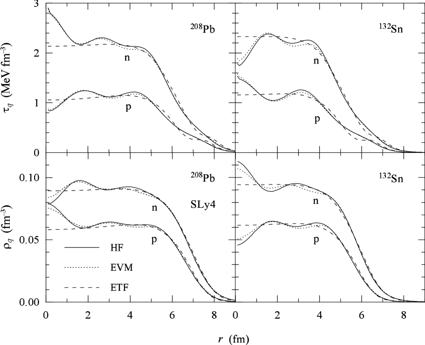
Figure 1: Comparison of the particle and kinetic energy densities for neutrons and protons in ²⁰⁸Pb and ¹³²Sn obtained with SLy4 in the HF, $\hbar^{4}$-order ETF and EVM approximations.

As a further illustration, Figure 1 displays the quantal HF particle and kinetic energy densities for neutrons and protons calculated in ²⁰⁸Pb and ¹³²Sn with SLy4, as well as the results of the ETF-$\hbar^{4}$ and EVM approximations. Figure 2 is a complementary plot showing the densities for ²⁰⁸Pb in the outer surface region on a semi-logarithmic scale. One can compare the exponential fall-off of the HF and EVM densities with the $1/r^{6}$ behaviour of the ETF-$\hbar^{4}$ solution at large distances.

4 Finite range forces

Now we turn our attention to the discussion of finite range forces as applied to semiclassical HF calculations. We will consider here an effective nucleon-nucleon force of Gogny type [2]. It consists of a central finite range part together with zero-range density-dependent and spin-orbit contributions:

$$v(s) = \sum_{i=1}^{2}[(w_{i}+\frac{b_{i}}{2}P^{\sigma}-\frac{h_{i}}{2}P^{\tau}-\frac{m_{i}}{4}P^{\sigma}P^{\tau})\tilde{w}_{i}(s)]$$ (45)

$$+ \frac{1}{6}t_{3}(1+x_{3}P^{\sigma})[\rho(\mbox{\boldmath$R$})]^{\alpha}\delta(\mbox{\boldmath$s$})+iW_{0}(\mbox{\boldmath$\sigma$}_{1}+\mbox{\boldmath$\sigma$}_{2})\hat{\mbox{\boldmath$k^{\prime}$}}\times\delta(\mbox{\boldmath$s$})\hat{\mbox{\boldmath$k$}},$$

where $w_{i}$, $m_{i}$, $b_{i}$ and $h_{i}$ are the usual exchange parameters of the central force and $\tilde{w}_{i}(s)=\exp(-s^{2}/\mu_{i}^{2})$ are the Gaussian form factors. The contributions of the zero-range and spin-orbit parts of (45) to the HF energy and single-particle potential (SPP) are the same as for the Skyrme force described in the previous section. Therefore, in the following we will concentrate only on the contributions to the energy and SPP associated with the finite range part of (45).

In the ETF approximation the HF energy is given by eq. (34) which yields the SPP potential through the variational principle. For the Gogny force the direct potential is given by [27]

$$V_{q}^{H}(\mbox{\boldmath$R$}) = \sum_{i=1}^{2}\frac{\pi\mu_{i}^{2}}{R}\int_{0}^{\infty}drr[\exp(-\frac{(R-r)^{2}}{\mu_{i}^{2}})-\exp(-\frac{(R+r)^{2}}{\mu_{i}^{2}})]$$ (46)

$$\mbox{}\times[(w_{i}+\frac{b_{i}}{2})\rho(r)-(h_{i}+\frac{m_{i}}{2})\rho_{q}(r)].$$

The $\hbar^{0}$ order exchange energy is given by [27]

$$\varepsilon_{ex}^{0}(\mbox{\boldmath$R$})=-\sum_{i=1}^{2}\frac{1}{6\pi^{2}\mu_{i}^{3}}\{X_{e,1,i}[v_{i}(k_{Fn},k_{Fn})+v_{i}(k_{Fp},k_{Fp})]-2X_{e,2,i}v_{i}(k_{Fn},k_{Fq})\},$$ (47)

where $X_{e,i,1}=w_{i}/2+b_{i}-h_{i}/2-m_{i}$ and $X_{e,2,i}=h_{i}/2+m_{i}$. The functions $v_{i}(k_{Fq},k_{Fq^{\prime}})$ read

$$v_{i}(k_{Fq},k_{Fq^{\prime}}) = \mu_{i}^{3}(k_{Fq}+k_{Fq^{\prime}})(k_{Fq}^{2}+k_{Fq^{\prime}}^{2}-k_{Fq}k_{Fq^{\prime}}){\rm erf}[\frac{\mu_{i}(k_{Fq}+k_{Fq^{\prime}})}{2}]$$ (48)

$$- \mu_{i}^{3}(k_{Fq}-k_{Fq^{\prime}})(k_{Fq}^{2}+k_{Fq^{\prime}}^{2}+k_{Fq}k_{Fq^{\prime}}){\rm erf}[\frac{\mu_{i}(k_{Fq}-k_{Fq^{\prime}})}{2}]$$

$$+ \frac{2}{\sqrt{\pi}}[\mu_{i}^{2}(k_{Fq}^{2}+k_{Fq^{\prime}}^{2}-k_{Fq}k_{Fq^{\prime}})-2]\exp[-\frac{\mu_{i}^{2}(k_{Fq}+k_{Fq^{\prime}})^{2}}{4}]$$

$$- \frac{2}{\sqrt{\pi}}[\mu_{i}^{2}(k_{Fq}^{2}+k_{Fq^{\prime}}^{2}+k_{Fq}k_{Fq^{\prime}})-2]\exp[-\frac{\mu_{i}^{2}(k_{Fq}-k_{Fq^{\prime}})^{2}}{4}].$$

The $\hbar^{0}$ order exchange potential in phase space is

$$V_{q}^{F}(\mbox{\boldmath$R$},k)=-\sum_{i=1}^{2}[X_{e,1,i}u_{i}(k,k_{Fq})-X_{e,2,i}u_{i}(k,k_{Fq^{\prime}})],$$ (49)

where the functions $u_{i}(k,k_{Fq})$ read

$$u_{i}(k,k_{Fq}) = {\rm erf}[\frac{\mu_{i}(k+k_{Fq})}{2}]-{\rm erf}[\frac{\mu_{i}(k-k_{Fq})}{2}]$$ (50)

$$+ \frac{2}{\sqrt{\pi}\mu_{i}k}(\exp[-\frac{\mu_{i}^{2}(k+k_{Fq})^{2}}{4}]-\exp[-\frac{\mu_{i}^{2}(k-k_{Fq})^{2}}{4}]).$$

It follows that the inverse of the momentum and position dependent effective mass (27) needed to compute the $\hbar^{2}$ contributions to the kinetic and exchange energy densities is

$$f_{q}(\mbox{\boldmath$R$},k)=1+\frac{m}{\hbar^{2}k}\sum_{i=1}^{2}[X_{e,1,i}\frac{\partial u_{i}(k,k_{Fq})}{\partial k}-X_{e,2,i}\frac{\partial u_{i}(k,k_{Fq^{\prime}})}{\partial k}].$$ (51)

With the help of eqs. (46), (47) and (51) the full energy density (34) plus the $t_{3}$ contribution of (38) can be written. Next, from this functional one should derive the ETF variational equations. This implies some lengthy algebra that can be partially avoided as follows. As shown in ref. [16], one obtains almost the same ETF-$\hbar^{2}$ energy if the full one-body semiclassical density matrix (29) is replaced by the one corresponding to a local potential (i.e., dropping all the space and momentum derivatives of $f$ in eq. (29) for the density matrix). With this simplification the kinetic energy density (30), which also appears in the $\hbar^{2}$ contribution to the exchange energy density, reduces to the one corresponding to a local potential. We use here this approximate way for deriving the variational equations. Once these equations have been solved, we compute the energy using the complete expression of the energy density.

The semiclassical ETF-$\hbar^{2}$ binding energies and r.m.s. radii obtained with the Gogny force D1 for some selected magic nuclei are reported in Table 2, which compares them with the quantal HF values. Usually, HF calculations with Gogny forces are carried out taking into account the two-body part of the center-of-mass correction. In the semiclassical framework one finds that the two-body correction exactly cancels the one-body part [13]. Thus, we have not included the center-of-mass correction in the semiclassical results presented in Table 2. It is also known that the ETF approximation at order $\hbar^{2}$ overbinds the nuclei and gives smaller r.m.s. radii than the HF ones [13, 14, 26]. These trends are followed in general by the semiclassical results with the D1 force as seen from Table 2.

One possible way to recover quantal effects, which are absent in the ETF approach described above, consists in considering the $\hbar^{2}$ exchange energy density as the exchange-correlation energy density in the Kohn-Sham scheme, and solving for each single-particle state the corresponding local Schrödinger equation (7). For this purpose, we replace $\rho$ and $\tau$ in the semiclassical exchange energy density (32) by the Kohn-Sham ansatz given by eqs. (5) and (6), which allows us to write the corresponding KS equations including effective mass and spin-orbit contributions that are similar to the HF equations for Skyrme forces.

To illustrate this approach we report in Table 3 our KS binding energies for tin isotopes in comparison with the HF values given in ref. [2], which do not include the two-body center-of-mass correction. We realize that our KS-$\hbar^{2}$ binding energies nicely reproduce the HF energies, the discrepancies being less than 2 MeV in this region of tin isotopes. For comparison, we also present in Table 3 the KS-$\hbar^{0}$ results from ref. [27] (where only the Slater term of the binding energy is taken as exchange-correlation energy). We can see that taking into account the $\hbar^{2}$-order corrections in our KS approach clearly improves the KS-$\hbar^{0}$ results.

Conclusions

In this paper we have reviewed the ETF approach to the HF method. From a theoretical point of view, we have derived the semiclassical binding energy for a non-local potential related with a finite range effective interaction, starting from the corresponding ETF density matrix up to order $\hbar^{2}$. As a limiting case, one recovers for Skyrme forces the usual expression for the kinetic energy density.

As a first numerical example, we have presented some ETF calculations of binding energies and r.m.s. radii of some magic nuclei using a recently proposed parametrization of the Skyrme force (SLy4). These semiclassical calculations have been carried out including corrections of order $\hbar^{4}$. These ETF binding energies are close to the HF ones and are similar to the ones obtained using a Strutinsky smoothing procedure. To recover the shell effects absent in the semiclassical calculation, one can use the expectation value method. It basically consists in performing one quantal iteration on top of the semiclassical calculation. In this way one reproduces the HF results with an accuracy around 0.5% for all the studied nuclei.

Finally, we have performed semiclassical ETF calculations of binding energies to order $\hbar^{2}$ using the finite range D1 Gogny force. These energies overbind the HF results by an amount around 3.5%, as it happens in the case of zero range Skyrme forces if the semiclassical calculation is taken only to second order in $\hbar$. We have also used the ETF-$\hbar^{2}$ exchange energy density as an exchange-correlation energy density within the Kohn-Sham scheme. In this case, we find that the KS binding energies reproduce almost perfectly the HF energies in the region of tin isotopes studied.

Table 1

The quantal HF binding energies (in MeV) and r.m.s. neutron and proton radii (in fm) of double closed shell nuclei for the Skyrme interaction SLy4 are compared with the results of the semiclassical $\hbar^{4}$-order ETF calculation and of the EVM discussed in the text.

		16O	40Ca	48Ca	56Ni	78Ni	100Sn	132Sn	208Pb
$B$:	HF	128.3	344.2	417.9	483.4	643.9	828.8	1103.8	1636.1
	EVM	127.6	342.9	416.3	480.4	642.2	825.8	1102.0	1634.3
	ETF-$\hbar^{4}$	128.7	348.8	422.8	488.1	645.5	826.9	1098.4	1629.9
$r_{\rm n}$:	HF	2.71	3.39	3.63	3.67	4.22	4.36	4.90	5.63
	EVM	2.66	3.34	3.63	3.70	4.25	4.38	4.92	5.64
	ETF-$\hbar^{4}$	2.66	3.34	3.61	3.67	4.25	4.36	4.91	5.62
$r_{\rm p}$:	HF	2.74	3.44	3.47	3.72	3.93	4.44	4.68	5.46
	EVM	2.69	3.39	3.45	3.75	3.96	4.46	4.70	5.48
	ETF-$\hbar^{4}$	2.68	3.38	3.46	3.72	3.94	4.44	4.69	5.48

Table 2

Binding energies (in MeV) and r.m.s. neutron and proton radii (in fm) for the D1 Gogny interaction. The HF binding energies are from ref. [29] and the HF radii from ref. [2].

		16O	40Ca	48Ca	90Zr	208Pb
$B$:	HF	127	338	411	779	1633
	ETF-$\hbar^{2}$	123.9	350.0	424.8	807.3	1670.9
$r_{\rm n}$:	HF	2.63	3.34	3.38	4.24	5.53
	ETF-$\hbar^{2}$	2.57	3.28	3.54	4.22	5.53
$r_{\rm p}$:	HF	2.65	3.38	3.38	4.18	5.40
	ETF-$\hbar^{2}$	2.58	3.32	3.43	4.18	5.44

Table 3

Binding energies (in MeV) of tin isotopes in the KS-$\hbar^{0}$, KS-$\hbar^{2}$ and HF calculations for the D1 Gogny interaction. The KS-$\hbar^{0}$ values are from ref. [27] and the HF values are from ref. [2].

		KS-$\hbar^{0}$		KS-$\hbar^{2}$		HF
112Sn		940.71		949.42		948.30
114Sn		958.48		969.56		968.40
116Sn		976.02		986.96		985.70
118Sn		991.81		1003.27		1002.16
120Sn		1007.40		1019.77		1018.90
122Sn		1022.81		1033.30		1032.19
124Sn		1038.04		1047.10		1045.90
132Sn		1098.22		1105.03		1102.77

Figure 2: Semi-logarithmic plot of the densities of Figure 1 for ²⁰⁸Pb in the outer surface region.

References

• [1] T.H.R. Skyrme, Phil. Mag. 1 (1956) 1043; Nucl. Phys. 9 (1959) 615; D. Vautherin and D.M. Brink, Phys. Rev. C5 (1972) 626.
• [2] J. Dechargé and D. Gogny, Phys. Rev. C21 (1980) 1568.
• [3] A.M. Kobos, B.A. Brown, P.E. Hodgson, G.R. Satchler and A. Budzanowsky, Nucl.Phys. A384 65; A.M. Kobos, B.A. Brown, R. Lindsay and G.R. Satchler Nucl.Phys. A425 (1984) 205; Dao T. Khoa and W. von Oertzen Phys. Lett. B304 8.
• [4] Li Guo-Qiang, J. Phys. G17 (1991) 1.
• [5] P. Hohenberg and W. Kohn Phys. Rev. A136 (1964) B864.
• [6] W. Kohn and L.J. Sham, Phys. Rev. A140 (1965) A1133.
• [7] I.Zh. Petkov and M.V. Stoitsov, Nuclear Density Functional Theory (Clarendon Press, Oxford, 1991).
• [8] W.D. Myers, Droplet Model of Atomic Nuclei (Plenum, New York, 1977); W.D. Myers and W. Swiatecki, Ann. Phys. (N.Y.) 55 (1969) 395; Ann. Phys. (N.Y.) 84 (1974) 186.
• [9] V.M. Strutinsky, Nucl. Phys. A122 (1968) 1; Nucl. Phys. A218 (1974) 169.
• [10] M. Brack, J. Damgård, A.S Jensen, H.C. Pauli, V.M. Strutinsky and C.Y. Wong, Rev. Mod. Phys. 44 (1972) 320.
• [11] M. Brack and P. Quentin, Phys. Lett. B56 (1975) 421.
• [12] B. Grammaticos and A. Voros, Ann. Phys. (N.Y.) 123 (1979) 359; Ann. Phys. (N.Y.) 129 (1980) 153.
• [13] M. Brack, C. Guet and H.-B. Håkansson, Phys. Rep. 123 (1985) 275.
• [14] M. Centelles, M. Pi, X. Viñas, F. Garcias and M. Barranco, Nucl. Phys. A510 (1990) 397.
• [15] M. Centelles, X. Viñas, M. Durand, P. Schuck and D. Von-Eiff, Ann. Phys. (N.Y.) A266 (1998) 207.
• [16] V.B Soubbotin and X. Viñas, nucl-th./9902039.
• [17] E. Chabanat, P. Bonche, P. Haensel, J. Meyer and R. Schaeffer, Nucl. Phys. A635 (1998) 231.
• [18] J.W. Negele and D. Vautherin, Phys. Rev. C5 (1972) 1472; C11 (1975) 1031.
• [19] X. Campi and A. Bouyssy, Phys. Lett. B73 (1978) 263; Nukleonica 24 (1979) 1.
• [20] E. Wigner, Phys. Rev. 40 (1932) 749; J.G. Kirkwood Phys. Rev. 44 (1933) 41; G.E. Uhlenbeck and and E. Beth, Physica 3 (1936) 729.
• [21] R.K. Bhaduri and C.K. Ross, Phys.Rev.Lett 29 (1971) 606; B.K. Jennings and R.K. Bhaduri, Nucl.Phys. A237 (1975) 149; B.K. Jennings, R.K. Bhaduri and M. Brack Phys. Rev. Lett 35 (1975) 228; Nucl. Phys. A253 (1975) 29.
• [22] D.A. Kirzhnits, Field Theoretical Methods in Many-Body Systems, (Pergamon, Oxford, 1967).
• [23] P. Ring and P. Schuck, The Nuclear Many-Body Problem, (Springer, New York, 1980).
• [24] M. Brack, Helvetia Physica Acta 58 (1985) 715.
• [25] M. Brack, B.K. Jennings and Y.H. Chu, Phys. Lett B65 (1976) 1; C. Guet and M. Brack, Z. Phys. A297
• [26] O. Bohigas, X. Campi, H. Krivine and J. Treiner Phys. Lett. 64B (1978) 381.
• [27] V.B. Soubbotin, X. Viñas, Ch. Roux, P.B. Danilov and K.A. Gridnev, J. Phys. G21 (1995) 947.
• [28] M. Brack and R.K. Bhaduri, Semiclassical Physics, (Addison-Wesley, Reading, 1997).
• [29] J. Meyer, J. Bartel, M. Brack, P. Quentin and S. Aicher, Phys. Lett. B172 (1986) 122.