Singularities and Conjugate Points in FLRW Spacetimes

Abstract

Conjugate points play an important role in the proofs of the singularity theorems of Hawking and Penrose. We examine the relation between singularities and conjugate points in FLRW spacetimes with a singularity. In particular we prove a theorem that when a non-comoving, non-spacelike geodesic in a singular FLRW spacetime obeys conditions (39) and (40), every point on that geodesic is part of a pair of conjugate points. The proof is based on the Raychaudhuri equation. We find that the theorem is applicable to all non-comoving, non-spacelike geodesics in FLRW spacetimes with non-negative spatial curvature and scale factors that near the singularity have power law behavior or power law behavior times a logarithm. When the spatial curvature is negative, the theorem is applicable to a subset of these spacetimes.

I Introduction

Hawking and Penrose proved that under very general physical conditions a spacetime has a singularity (Hawking:1969sw, ; hawking1973large, ). A singularity is defined as a non-spacelike geodesic that is incomplete. One uses this definition because test particles move on these trajectories and thus have only traveled for a finite proper time. The rough idea of the proof of these singularity theorems is that one assumes that all non-spacelike geodesics are complete, one has a trapped surface (e.g. an event horizon of a black hole) and that the weak energy condition is obeyed. Under these conditions it is shown that there must be conjugate points (which one can see as geodesics that are converging at two points) and that leads to a contradiction with the completeness of geodesics. Because of this relation between a singularity and conjugate points, it is sometimes said that having a singularity is equivalent to having conjugate points. This of course does not follow in any way from the theorems of Hawking and Penrose, but one can examine this idea in simple spacetimes. More specifically, we will do this in FLRW spacetimes, which describe isotropic and spatially homogeneous universes and are used as a model in cosmology. We prove that in a singular FLRW spacetime, every point on a non-comoving, non-spacelike geodesic satisfying conditions (39) and (40) is conjugate to another point of that geodesic. We will examine the conditions of the theorem for power law and logarithmic behavior of the scale factor. This includes in particular an FLRW spacetime with flat spatial three-surfaces that contains either a perfect homogeneous radiation fluid or a perfect homogeneous matter fluid. We show that the theorem is applicable to spacetimes with these scale factors when they have non-negative spatial curvature. For negative spatial curvature, the theorem is applicable to a subset of these scale factors.

In this paper we first give a brief recap of the theory used to study conjugate points, in particular the Raychaudhuri equation. We then use this equation to prove the theorem after which we show that the conditions of the theorem are obeyed for certain physical FLRW spacetimes with non-negative spatial curvature and for a subset of the physical spacetimes with negative spatial curvature. We adopt units in which the velocity of light $c=1.$

II Conjugate Points and the Raychaudhuri Equation

In this section we will recall the theory that is needed to study conjugate points. We will state two propositions without proofs, one can find these in e.g. (hawking1973large, ; beem1996global, ). Everything will be stated for a general spacetime $(M,g),$ where $g$ is a Lorentzian metric. The Riemann curvature tensor $R$ is defined by

$$R(X,Y)Z=\nabla_{X}(\nabla_{Y}Z)-\nabla_{Y}(\nabla_{X}Z)-\nabla_{[X,Y]}Z,$$ (1)

where $\nabla$ is the Levi-Civita connection. Contracting the curvature tensor, one can define the Ricci tensor $\mathrm{Ric}$ as the tensor with components

$$R_{\lambda\nu}=R_{\;\;\lambda\rho\nu}^{\rho}.$$ (2)

Covariant differentiation along a curve $\gamma(\tau)$ will be denoted by $D_{\tau}$.

Definition 1.

Let $\gamma:\>[\tau_{\mathrm{i}},\tau_{\mathrm{f}}]\rightarrow M$ be a non-spacelike geodesic segment. A variation through geodesics of $\gamma$ is a smooth function $\Gamma:\;(-\epsilon,\epsilon)\times[\tau_{\mathrm{i}},\tau_{\mathrm{f}}]\rightarrow M$, such that $\Gamma(0,\tau)=\gamma(\tau)$ for all $\tau\in[\tau_{\mathrm{i}},\tau_{\mathrm{f}}]$ and every curve $\Gamma(w_{0},\tau)$ is a geodesic segment. The variation field of $\Gamma$ is the vector field $J(\tau)=\partial_{w}\Gamma(w,\tau)|_{w=0}$ along $\gamma$.

Definition 2.

A vector field $J$ along a geodesic segment $\gamma:\;[\tau_{\mathrm{i}},\tau_{\mathrm{f}}]\rightarrow M$ that satisfies the Jacobi equation,

$$D_{\tau}^{2}J+R(J,\dot{\gamma})\dot{\gamma}=0,$$ (3)

where $\dot{\gamma}=D_{\tau}\gamma,$ will be called a Jacobi field.

Proposition 1.

Variations through geodesics $\Gamma$ of a geodesic segment $\gamma$ have a Jacobi field as variation field and every Jacobi field along $\gamma$ corresponds to a variation through geodesics.

From Eq. (3) it then follows that the Jacobi fields along a geodesic segment are determined by initial conditions $J(\tau_{0})$ and $D_{\tau}J(\tau_{0})$ at $\gamma(\tau_{0})$ and thus form an eight dimensional subspace of the space of vector fields along $\gamma.$

II.1 Timelike Geodesic Segment

We now first restrict to timelike geodesic segments $\gamma$.

Definition 3.

If $\gamma$ is a timelike geodesic segment joining $p,q\in\gamma$, $p$ is said to be conjugate to $q$ along $\gamma$ if there exists a non-vanishing Jacobi field $J$ along $\gamma$ such that $J$ is zero at $p$ and $q$.

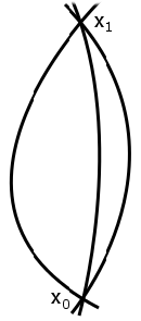
Figure 1: Let the lines be geodesics of some two-dimensional manifold. Then $x_{0}$ and $x_{1}$ are conjugate to each other.

In figure 1 one can find an illustration to give some idea of conjugate points. Jacobi fields corresponding to conjugate points necessarily live in $N(\gamma),$ the space of vector fields along $\gamma$ that are orthogonal to $\dot{\gamma}.$ In the theorem that we prove in section III.2, our goal is to show that there exists a conjugate point to a certain fixed point on a geodesic. To do this we only have to look at the Jacobi fields that are orthogonal to $\dot{\gamma}$ and vanish at this initial point. This means that we can restrict to a three dimensional vector space of Jacobi fields. To describe all of these fields at once, we will introduce Jacobi tensors. We first simplify notation by defining

$$R_{\gamma}(v) = R\left(v,\dot{\gamma}(\tau)\right)\dot{\gamma}(\tau).$$ (4)

Let $A:\;N(\gamma)\rightarrow N(\gamma)$ be a smooth tensor field. Since $g\left(R_{\gamma}\left(v\right),\dot{\gamma}(\tau)\right)=0$ we can define a map $R_{\gamma}A:\>N(\gamma(\tau))\rightarrow N(\gamma(\tau))$ by

$$R_{\gamma}A(\tau)(v) = R_{\gamma}\left(A(\tau)(v)\right).$$ (5)

Definition 4.

A smooth $(1,1)$ tensor field $A:\;N(\gamma)\rightarrow N(\gamma)$ is called a Jacobi tensor field if it satisfies

$$D_{\tau}^{2}A+R_{\gamma}A = 0,$$ (6)

$$\mathrm{Ker}(A(\tau))\cap\mathrm{Ker}(D_{\tau}A(\tau)) = \{0\}$$ (7)

for all $\tau\in[\tau_{\mathrm{i}},\tau_{\mathrm{f}}]$. Here $\mathrm{Ker}(A(\tau))$ is the kernel of $A(\tau)$.

If $V\in N(\gamma)\backslash\{0\}$ is a parallel transported vector field along $\gamma$, i.e. $D_{\tau}V=0,$ and $A(\tau)$ a Jacobi tensor field, define $J(\tau)=A(\tau)V(\tau)$. Then $J(\tau)$ is a Jacobi field. Condition (7) guarantees that $J$ is non-trivial. Therefore $A$ can be seen as describing different families of geodesics at the same time. We now define a Jacobi tensor field that describes all solutions to Eq. (3) living in $N(\gamma)$ and that vanish at $\gamma(\tau_{\mathrm{i}})$:

Definition 5.

Let $\{E_{\mu}\}$, $\mu=0,1,2,3$ be a parallel transported orthonormal frame along $\gamma$ such that $E_{0}=\dot{\gamma}$. Let $J_{i}(\tau),$ $i\in\{1,2,3\},$ be the Jacobi field with $J_{i}(\tau_{\mathrm{i}})=0$ and $D_{\tau}J_{i}(\tau_{\mathrm{i}})=E_{i}(\tau_{\mathrm{i}})$. Let $A$ be the tensor such that the components in the basis $E_{\mu}$ are given by

$$A_{\;\;l}^{k}(\tau) = (J_{l}(\tau))^{k};$$ (8)

$$A_{\;\;0}^{0}=A_{\;\;0}^{k}=A_{\;\;l}^{0} = 0,$$

for $k,l=1,2,3$.

If $A$ is singular for some $\tau$ this will correspond to a Jacobi field that vanishes at that $\gamma(\tau),$ hence that point on the geodesic is conjugate to $\gamma(\tau_{\mathrm{i}}).$ So points conjugate to $\gamma(\tau_{\mathrm{i}})$ are the points where $\det A=0.$ To examine whether $A$ is singular at some point, we develop some more machinery.

Definition 6.

Let $B_{A}=\left(D_{\tau}A\right)A^{-1}$ at points where $\det A\neq 0$

1. The expansion $\theta_{A}$ is

   $$\theta_{A}=\mathrm{tr}(B_{A}).$$ (9)

2. The vorticity tensor $\omega_{A}$ is

   $$\omega_{A}=\frac{1}{2}(B_{A}-B_{A}^{\dagger}).$$ (10)

3. The shear tensor $\sigma_{A}$ is

   $$\sigma_{A}=\frac{1}{2}(B_{A}+B_{A}^{\dagger})-\frac{\theta_{A}}{3}I,$$ (11)

   where $I$ is the identity matrix.

Notice that

$$B_{A}=\omega_{A}+\sigma_{A}+\frac{\theta_{A}}{3}I.$$ (12)

Proposition 2.

The vorticity

$$\omega_{A}=0,$$ (13)

the expansion

$$\theta_{A}=\partial_{\tau}\log\left(\det A\right)$$ (14)

and the derivative of $\theta_{A}$ is given by

$$\dot{\theta}_{A}=-\mathrm{Ric}(\dot{\gamma}(\tau),\dot{\gamma}(\tau))-\mathrm{tr}(\sigma_{A}^{2})-\frac{\theta_{A}^{2}}{3}.$$ (15)

Eq. (15) is also called the Raychaudhuri equation for timelike geodesics.

II.2 Null Geodesic Segment

For null geodesic segments $\gamma:\;[\tau_{\mathrm{i}},\tau_{\mathrm{f}}]\rightarrow M$ one can also define conjugate points using Jacobi fields. However now $\dot{\gamma}\in N(\gamma)$, so since we will be interested in the convergence of geodesics, it makes more sense to look at the projection of Jacobi fields to a quotient space formed by identifying vectors that differ by a multiple of $\dot{\gamma}.$ This idea is implicitly used in (hawking1973large, ) and further developed in (Bolts, ). One can do a similar analysis as for the timelike case and define Jacobi classes $\bar{J}$, Jacobi tensor fields $\bar{A}$, vorticity $\bar{\omega}_{\bar{A}},$ shear $\bar{\sigma}_{\bar{A}}$ and expansion $\bar{\theta}_{\bar{A}}$ for this quotient space. One can derive that

$$\bar{\theta}_{\bar{A}}=\partial_{\tau}\log\left(\det\bar{A}\right)$$ (16)

and derive a Raychaudhuri equation which is given by

$$\partial_{\tau}\bar{\theta}_{\bar{A}}=-\mathrm{Ric}(\dot{\gamma},\dot{\gamma})-\mathrm{tr}(\bar{\sigma}_{\bar{A}}^{2})-\frac{\bar{\theta}_{\bar{A}}^{2}}{2}.$$ (17)

Points conjugate to $\gamma(\tau_{\mathrm{i}})$ correspond to points where $\det\bar{A}=0,$ with $\bar{A}$ a specific Jacobi tensor field constructed for a null geodesic as $A$ in (8) for a timelike geodesic.

III FLRW Spacetimes

We would like to study the relation between conjugate points and a singularity in a spacetime with an FLRW metric. This metric describes a spatially homogeneous, isotropic spacetime and in spherical coordinates it is given by:

$$ds^{2}=-dt^{2}+a(t)^{2}\left[\frac{dr^{2}}{1-\kappa r^{2}}+r^{2}\left(d\theta^{2}+\sin^{2}(\theta)d\varphi^{2}\right)\right],$$ (18)

where $\kappa$ is the curvature of spacelike three-surfaces and the scale factor $a(t)$ is normalized such that $a(t_{1})=1$ for some time $t_{1}$. This metric is a good description of our universe, since from experiments as WMAP and Planck, it follows that our universe is spatially homogeneous and isotropic when averaged over large scales. Geodesics $\gamma(\tau)$, where $\tau$ is an affine parameter, satisfy

$$\frac{d\gamma^{0}}{d\tau}=\frac{\sqrt{C-\epsilon_{\mathrm{n}}a^{2}}}{a},$$ (19)

where $C=|\vec{V}(t_{1})|^{2}=g_{ij}\dot{\gamma}^{i}\dot{\gamma}^{j}(t_{1})$ and $\epsilon_{\mathrm{n}}$ is the normalization of the geodesic: $\epsilon_{\mathrm{n}}=0$ for null geodesics and $\epsilon_{\mathrm{n}}=-1$ for timelike geodesics. As argued in (Lam:2016kmt, ), singularities (which are in general defined as incomplete non-spacelike geodesics) in this spacetime are the points where the scale factor $a$ vanishes. We would like to prove that under certain conditions a singularity implies that all points on a geodesic are part of a pair of conjugate points.

III.1 Examining the Definition of Conjugate Points

Since the metric (18) becomes degenerate at a singularity we can try to generalize the definition of conjugate points to also include these points. For the theorem this will be important because we will only be able to show that a certain point $\gamma(t)$ is conjugate to a point $\gamma(t^{\prime})$ where $t_{0}\leq t^{\prime}<t$ and $t_{0}$ corresponds to the singularity $a(t_{0})=0$. Let us examine a specific model. We will study the FLRW metric with $\kappa=0$ and $a(t)=\sqrt{t}.$ This models a spatially flat universe with a perfect radiation fluid for which the energy density $\rho\propto 1/a^{4}$ and is consistent with current observations (Ade:2015xua, ). To derive the geodesics we use Cartesian coordinates for the metric (18)

$$ds^{2}=-dt^{2}+a(t)^{2}\left(dx^{i}\right)^{2}.$$ (20)

Let a geodesic be given by $\gamma(\tau)=\left(t(\tau),x^{i}(\tau)\right)$ and let $u^{\mu}=d\gamma^{\mu}/d\tau$. The geodesic equations are given by

$$\frac{du^{0}}{d\tau}+a\dot{a}\left(u^{i}\right)^{2} = 0$$

$$\frac{du^{i}}{d\tau}+2\frac{\dot{a}}{a}u^{0}u^{i} = 0.$$ (21)

The second equation can be rewritten as

$$\frac{d}{d\tau}\left[a^{2}u^{i}\right]=0$$ (22)

with solution

$$u^{i}=\frac{C_{i}}{a^{2}},$$ (23)

where $C_{i}$ are constants. The constraint equation is

$$\epsilon_{\mathrm{n}}=-\left(u^{0}\right)^{2}+a^{2}\left(u^{i}\right)^{2}$$ (24)

and leads to

$$u^{0}=\frac{\sqrt{C-\epsilon_{\mathrm{n}}a^{2}}}{a},$$ (25)

(Eq. (19)) where $C=\sum_{i}C_{i}^{2}$. Let us now consider timelike geodesics, $\epsilon_{\mathrm{n}}=-1$ and choose $C=1$. We can then solve Eq. (25) for $a(t)=\sqrt{t}$ by

$$\sqrt{t+t^{2}}-\sinh^{-1}\left(\sqrt{t}\right)=\tau,$$ (26)

where we chose $\tau$ such that $\tau=0$ at the singularity. From Eqs. (23) and (25) we find that

$$\frac{dx^{i}}{dt}=\frac{1}{\sqrt{1+a^{2}}}\frac{C_{i}}{a},$$ (27)

which is solved by

$$x^{i} = 2C_{i}\sinh^{-1}\left(\sqrt{t}\right)+D_{i},$$ (28)

where $D_{i}$ are constants (notice that we have the restriction $1=\sum_{i}C_{i}^{2}$). We consider the geodesic

$$\gamma=\left(t,2\sinh^{-1}\left(\sqrt{t}\right),0,0\right)$$ (29)

and we want to examine conjugate points along this geodesic. We now construct the matrix $A$ of Eq. (8) corresponding to the point $\gamma(t_{2})$ for this geodesic. An orthonormal basis that is parallel transported along this geodesic is given by

$$E_{0} = \left(\sqrt{\frac{1+t}{t}},\frac{1}{t},0,0\right)$$

$$E_{1} = \left(\frac{1}{\sqrt{t}},\frac{\sqrt{1+t}}{t},0,0\right)$$

$$E_{2} = \left(0,0,\frac{1}{\sqrt{t}},0\right)$$

$$E_{3} = \left(0,0,0,\frac{1}{\sqrt{t}}\right).$$ (30)

We now need the Jacobi fields $J_{i}$ for $i\in\{1,2,3\}$ such that $J_{i}(t_{2})=0$ and $D_{\tau}J_{i}(t_{2})=E_{i}(t_{2})$. The differential equations (3) for the first 2 components of the Jacobi fields only depend on each other. The differential equation for $J_{i}^{k}$, $k\in\{2,3\}$ is given by

$$\frac{(1+2t)\left(J_{i}^{k}\right)^{\prime}+2t(1+t)\left(J_{i}^{k}\right)^{\prime\prime}}{t}=0.$$ (31)

This implies that

$$J_{1} = \left(h_{1}(t),h_{2}(t),0,0\right)$$

$$J_{2} = \left(0,0,h_{3}(t),0\right)$$ (32)

$$J_{3} = \left(0,0,0,h_{3}(t)\right).$$

We can solve Eq. (31) for $h_{3}$ explicitly and find

$$h_{3}(t)=-2\sqrt{t_{2}}\left(\sinh^{-1}\left(\sqrt{t_{2}}\right)-\sinh^{-1}\left(\sqrt{t}\right)\right).$$ (33)

We have to solve for $h_{1}$ and $h_{2}$ numerically. The matrix $A$ is then given by

$$A=\left(\begin{array}[]{ccc}-\frac{1}{\sqrt{t}}h_{1}+\sqrt{1+t}h_{2}&0&0\\ 0&\sqrt{t}h_{3}&0\\ 0&0&\sqrt{t}h_{3}\end{array}\right),$$ (34)

which has determinant

$$\det A=t\left(-\frac{1}{\sqrt{t}}h_{1}+\sqrt{1+t}h_{2}\right)h_{3}^{2}.$$ (35)

Notice that at $t=0$, $\sqrt{t}h_{3}(t)=0$, which naively would mean that $\gamma(t_{2})$ is conjugate to the point at the singularity. However, in other coordinate systems the Jacobi field does not vanish (see Eq. (33)). This behavior is caused by the degeneracy of the metric at the singularity. The norm of the Jacobi field however, is zero in both coordinate systems.

We use this example as a motivation to generalize the definition of a conjugate point to include points where the metric is degenerate. From a physical point of view it is the norm of the Jacobi field that matters since this corresponds to the distance between particles moving on nearby geodesics. That is why we will also say that we have conjugate points on a timelike geodesic when the norm of the Jacobi field vanishes. Such a Jacobi field should still be perpendicular to the geodesic (otherwise one could just get that it is a null vector). As long as the metric is non-degenerate this definition is the same as our original definition. Notice that the vanishing of the determinant of the matrix $A$ is equivalent to a Jacobi field $J$ perpendicular to $\dot{\gamma}$ and such that $g(E_{i},J)=0$ for all $i$. From

$$g(J,J)=\sum_{i}g(E_{i},J)^{2}$$ (36)

we conclude that $g(E_{i},J)=0$ for all $i$ is equivalent to $g(J,J)=0.$

With this new definition two points on a geodesic can be conjugate in two different ways. The first one is that geodesics are indeed converging to one point (to first order), the second one is that that does not happen, but that the norm of the Jacobi field vanishes. We found that the vanishing of the determinant of $A$ is equivalent to this new definition if the Jacobi field is perpendicular to the geodesic. In the same way one can give a generalized definition of conjugate points for null geodesics.

III.2 The Theorem

We will now prove the theorem that states that when a certain non-comoving, non-spacelike geodesic satisfies conditions (39) and (40), every point on that geodesic is part of a pair of conjugate points. Here we do not know whether geodesics actually converge to that point. To prove this for a point $\gamma(t_{2})$ on a timelike geodesic, the idea is to use Eqs. (14) and (15) to derive an inequality for $\log\left(\det A(t)\right).$ From this inequality we show that $\log\left(\det A(t)\right)$ goes to $-\infty$ at a point $\gamma(t^{\prime})$ that lies in between the singularity and $\gamma(t_{2}).$ This means that $\det A(t^{\prime})=0$ which implies that $\gamma(t^{\prime})$ is conjugate to $\gamma(t_{2}).$ For null-geodesics we use the same strategy using Eqs. (16) and (17).

.

Theorem.

Let $\gamma(\tau(t))$ be a non-comoving ($C>0$), non-spacelike geodesic in a spacetime with FLRW metric such that $a(t_{0})=0$ for a certain $t_{0}$ and $a$ is smooth for $t>t_{0}$. Let

$$f(t)=3\overset{..}{a}+2\frac{C}{a}\left[\frac{\overset{..}{a}}{a}-\frac{\dot{a}^{2}}{a^{2}}-\frac{\kappa}{a^{2}}\right]$$ (37)

and define

$$f_{+}(t) = \begin{cases}f(t)&\;\mbox{for t where }f(t)\geq 0\\ 0&\;\mbox{for t where }f(t)<0\end{cases}$$ (38)

$$f_{-}(t) = \begin{cases}-f(t)&\;\mbox{for t where }f(t)\leq 0\\ 0&\;\mbox{for t where }f(t)>0.\end{cases}$$

A point $\gamma(\tau(t_{2}))$ for $t_{2}\neq t_{0}$ is conjugate to a point $\gamma(\tau(t^{\prime}))$ where $t_{0}\leq t^{\prime}<t_{2}$ if the following conditions are satisfied:

$$\lim_{t\rightarrow t_{0}}\int_{t}^{t_{1}}a(t^{\prime})\int_{t^{\prime}}^{t_{1}}\frac{1}{a}\left[\frac{\overset{..}{a}}{a}-\frac{\dot{a}^{2}}{a^{2}}-\frac{\kappa}{a^{2}}\right]dt^{\prime\prime}dt^{\prime} = -\infty$$ (39)

$$\lim_{t\rightarrow t_{0}}\int_{t}^{t_{1}}f_{+}dt^{\prime} = \alpha\in\mathbb{R}_{\geq 0}$$ (40)

for a $t_{1}>t_{0}.$

Proof.

We will prove this separately for timelike and null geodesics. Let $\gamma$ be a timelike geodesic. Let $\gamma(\tau(t_{2}))$ be a point on this geodesic and let $A$ denote the Jacobi tensor field as defined in (8). To show that $\gamma(\tau(t_{2}))$ is conjugate to a point $\gamma(\tau(t^{\prime}))$ with $t_{0}\leq t^{\prime}<t$, we will show that $\log\left(\det A\right)$ has to go to $-\infty$ at some point $\gamma(t^{\prime}).$

Consider Eq. (19) and the Raychaudhuri equation, Eq. (15). Since $\sigma_{A}$ is symmetric we have that $\mathrm{tr}\left(\sigma_{A}^{2}\right)$ is positive such that

$$\frac{d\theta_{A}}{dt}=\frac{d\tau}{dt}\frac{d\theta_{A}}{d\tau}\leq\frac{-a}{\sqrt{C+a^{2}}}\mathrm{Ric}(\dot{\gamma}(\tau),\dot{\gamma}(\tau)).$$ (41)

For the FLRW metric we then find that

$$-\mathrm{Ric}(\dot{\gamma}(\tau),\dot{\gamma}(\tau))=3\frac{\overset{..}{a}}{a}+2\frac{C}{a^{2}}\left[\frac{\overset{..}{a}}{a}-\frac{\dot{a}^{2}}{a^{2}}-\frac{\kappa}{a^{2}}\right],$$ (42)

which results in

$$\frac{d\theta_{A}}{dt} \leq \frac{1}{\sqrt{C+a^{2}}}\left(f_{+}-f_{-}\right).$$ (43)

Notice that in conditions (39) and (40) we can assume that $t_{1}<t_{2}$ and that $\gamma(t_{1})$ is not conjugate to $\gamma(t_{2}).$ We find from condition (39) that:

$$\lim_{t\rightarrow t_{0}}\int_{t}^{t_{1}}a\int_{t^{\prime}}^{t_{1}}f_{+}dt^{\prime\prime}dt^{\prime}-\lim_{t\rightarrow t_{0}}\int_{t}^{t_{1}}a\int_{t^{\prime}}^{t_{1}}f_{-}dt^{\prime\prime}dt^{\prime}=-\infty.$$ (44)

From condition (40) it follows that

$$\int_{t}^{t_{1}}f_{+}dt^{\prime}$$ (45)

is a function that is $\alpha$ at $t_{0},$ $0$ at $t_{1}$ and strictly decreasing. Hence

$$a(t)\int_{t}^{t_{1}}f_{+}dt^{\prime}$$ (46)

is vanishing at $t_{0}$ and $t_{1}$ and continuous and positive in between. This implies that

$$\lim_{t\rightarrow t_{0}}\int_{t}^{t_{1}}a\int_{t^{\prime}}^{t_{1}}f_{+}dt^{\prime\prime}dt^{\prime}=\beta\in\mathbb{R}_{\geq 0}$$ (47)

and together with Eq. (44) this gives

$$\lim_{t\rightarrow t_{0}}\int_{t}^{t_{1}}a\int_{t^{\prime}}^{t_{1}}f_{-}dt^{\prime\prime}dt^{\prime} = \infty.$$ (48)

For $t<t_{1}$ we find with Eq. (43) that

$$\theta_{A}(t) = -\int_{t}^{t_{\text{1}}}\frac{d\theta_{A}}{dt}dt^{\prime}+\theta_{A}(t_{1})$$ (49)

$$\geq -\frac{1}{\sqrt{C}}\int_{t}^{t_{1}}f_{+}dt^{\prime}+\frac{1}{\sqrt{C+a_{\mathrm{max}}^{2}}}\int_{t}^{t_{1}}f_{-}dt^{\prime}+\theta_{A}(t_{1}),$$

where $a_{\mathrm{max}}=\max\{a(t)|t_{0}\leq t\leq t_{1}\}.$ Then using Eq. (14):

$$\log\left(\det A(t)\right) = -\int_{t}^{t_{1}}\frac{a}{\sqrt{C+a^{2}}}\theta_{A}dt^{\prime}+\log\left(\det A(t_{1})\right)$$ (50)

$$\leq \frac{1}{C}\int_{t}^{t_{1}}a\int_{t^{\prime}}^{t_{1}}f_{+}dt^{\prime\prime}dt^{\prime}-\frac{1}{C+a_{\mathrm{max}}^{2}}\int_{t}^{t_{1}}a\int_{t^{\prime}}^{t_{1}}f_{-}dt^{\prime\prime}dt^{\prime}$$

$$-\theta_{A}(t_{1})\int_{t}^{t_{1}}\frac{a}{\sqrt{C+a^{2}}}dt^{\prime}+\log\left(\det A(t_{1})\right).$$

With Eqs. (47) and (48) it then follows that the right-hand side of Eq. (50) goes to $-\infty$ in the limit $t\rightarrow t_{0}$. That means that $\gamma(\tau(t_{2}))$ is conjugate to a point $\gamma(\tau(t^{\prime}))$ with $t_{0}\leq t^{\prime}<t_{1}$.

Consider now a null geodesic $\gamma$ and let $\gamma(\tau(t_{2}))$ be a point on this geodesic. The Raychaudhuri equation, Eq. (17), reads:

$$\frac{d\bar{\theta}_{\bar{A}}}{dt} = \frac{a}{\sqrt{C}}\left(2\frac{C}{a^{2}}\left[\frac{\overset{..}{a}}{a}-\frac{\dot{a}^{2}}{a^{2}}-\frac{\kappa}{a^{2}}\right]-\mathrm{tr}\left(\bar{\sigma}_{\bar{A}}^{2}\right)-\frac{\bar{\theta}_{\bar{A}}^{2}}{2}\right)$$ (51)

$$\leq 2\frac{\sqrt{C}}{a}\left[\frac{\overset{..}{a}}{a}-\frac{\dot{a}^{2}}{a^{2}}-\frac{\kappa}{a^{2}}\right].$$

We can again assume that $t_{1}<t_{2}$ and that $\gamma(t_{1})$ is not conjugate to $\gamma(t_{2})$. It then follows that for $t<t_{1}$

$$\bar{\theta}_{\bar{A}}(t) = -\int_{t}^{t_{1}}\frac{d\bar{\theta}_{\bar{A}}}{dt}dt^{\prime}+\bar{\theta}_{\bar{A}}(t_{1})$$ (52)

$$\geq -2\sqrt{C}\int_{t}^{t_{1}}\frac{1}{a}\left[\frac{\overset{..}{a}}{a}-\frac{\dot{a}^{2}}{a^{2}}-\frac{\kappa}{a^{2}}\right]dt^{\prime}+\bar{\theta}_{\bar{A}}(t_{1}).$$

This implies that

$$\log\left(\det\bar{A}(t)\right) = -\int_{t}^{t_{1}}\frac{a}{\sqrt{C}}\bar{\theta}_{\bar{A}}dt^{\prime}+\log\left(\det\bar{A}(t_{1})\right)$$ (53)

$$\leq 2\int_{t}^{t_{1}}a\int_{t^{\prime}}^{t_{1}}\frac{1}{a}\left[\frac{\overset{..}{a}}{a}-\frac{\dot{a}^{2}}{a^{2}}-\frac{\kappa}{a^{2}}\right]dt^{\prime\prime}dt^{\prime}-\bar{\theta}_{\bar{A}}(t_{1})\frac{1}{\sqrt{C}}\int_{t}^{t_{1}}adt^{\prime}+\log\left(\det\bar{A}(t_{1})\right),$$

where we have used Eq. (16). Condition (39) then implies that the right-hand side of Eq. (53) goes to $-\infty$ in the limit $t\rightarrow t_{0}.$ Hence $\gamma(\tau(t_{2}))$ is conjugate to a point $\gamma(\tau(t^{\prime}))$ where $t_{0}\leq t^{\prime}<t_{1}$. ∎

Notice that one can rewrite condition (39) by partially integrating the first term such that one obtains

$$-\infty = \lim_{t\rightarrow t_{0}}\int_{t}^{t_{1}}a(t^{\prime})\int_{t^{\prime}}^{t_{1}}\frac{1}{a}\left[\frac{d}{dt}\frac{\dot{a}}{a}-\frac{\kappa}{a^{2}}\right]dt^{\prime\prime}dt^{\prime}$$ (54)

$$= \frac{\dot{a}(t_{1})}{a^{2}(t_{1})}\int_{t_{0}}^{t_{1}}adt^{\prime}-\log(a(t_{1}))+\lim_{t\rightarrow t_{0}}\log(a(t))+\lim_{t\rightarrow t_{0}}\int_{t}^{t_{1}}a(t^{\prime})\int_{t^{\prime}}^{t_{1}}\frac{\dot{a}^{2}-\kappa}{a^{3}}dt^{\prime\prime}dt^{\prime}.$$

Thus condition (39) is definitely satisfied when

$$\lim_{t\rightarrow t_{0}}\int_{t}^{t_{1}}a\int_{t^{\prime}}^{t_{1}}\frac{\dot{a}^{2}-\kappa}{a^{3}}dt^{\prime\prime}dt^{\prime}$$ (55)

is not $\infty.$

Also condition (40) is satisfied as soon as $f$ is negative for $t\in(t_{0},t_{0}+\delta),$ $\delta\ll 1$.

The theorem can be proven under different conditions. One set of such conditions would be for instance

$$\lim_{t\rightarrow t_{0}}\int_{t}^{t_{1}}\frac{a}{\sqrt{C+a^{2}}}\int_{t^{\prime}}^{t_{1}}\frac{1}{\sqrt{C+a^{2}}}\left(3\overset{..}{a}+2\frac{C}{a}\left[\frac{\overset{..}{a}}{a}-\frac{\dot{a}^{2}}{a^{2}}-\frac{\kappa}{a^{2}}\right]\right)dt^{\prime\prime}dt^{\prime} = -\infty;$$ (56)

$$\lim_{t\rightarrow t_{0}}\int_{t}^{t_{1}}a\int_{t^{\prime}}^{t_{1}}\frac{1}{a}\left[\frac{\overset{..}{a}}{a}-\frac{\dot{a}^{2}}{a^{2}}-\frac{\kappa}{a^{2}}\right]dt^{\prime\prime}dt^{\prime} = -\infty$$

which would have made the proof really easy.

III.3 Relation to Physical Spacetimes

The theorem is applicable to FLRW spacetimes with physically realistic scale factors. Notice that the conditions of the theorem only depend on the form of the scale factor $a(t)$ near the singularity. We will assume it there to take one of the forms

$$a(t) = t^{1/\epsilon}$$ (57)

$$a(t) = -t^{1/\epsilon}\log(t),$$ (58)

with $\epsilon>0$. Notice that in case of power law behavior (57),

$$\epsilon=-\frac{\dot{H}}{H^{2}}$$ (59)

is the principal slow roll parameter ($H=\dot{a}/a$ is the Hubble parameter). When $0<\epsilon\ll 1$ the scale factor (57) corresponds to inflation, $\epsilon=3/2$ gives the scale factor of an FLRW spacetime with $\kappa=0$ containing a perfect homogeneous matter fluid and $\epsilon=2$ gives the scale factor of an FLRW spacetime with $\kappa=0$ containing a perfect homogeneous radiation fluid. The second form (58) of the scale factor is related to one loop corrections. When matter is integrated out the effective action contains, up to boundary terms, terms $R^{2}\log(R/\mu^{2})$ and $W^{2}\log(R/\mu^{2}),$ where $W$ is the Weyl tensor and $\mu$ is an energy scale (Zeldovich:1971mw, ; Gurovich:1979xg, ; Barvinsky:1987uw, ; Barvinsky:1990up, ). This motivates to examine scale factors that have more complicated behavior near the singularity and that is why we also study the logarithmic behavior (58). Notice however that (Zeldovich:1971mw, ; Gurovich:1979xg, ) focussed mostly on anisotropic expansions which actually help to resolve the singularity. We will however still examine the form (58) since in the end it just serves as an example to what kind of scale factors the theorem can be applied.

We will consider both of the scale factors (57) and (58) separately, starting with the power law behavior. We find that for $\epsilon\notin\{1,3\}$

$$\int_{t}^{t_{1}}a\int_{t^{\prime}}^{t_{1}}\frac{1}{a}\left[\frac{\overset{..}{a}}{a}-\frac{\dot{a}^{2}}{a^{2}}-\frac{\kappa}{a^{2}}\right]dt^{\prime\prime}dt^{\prime} = \frac{\alpha\epsilon}{1+\epsilon}\left(t_{1}^{1/\epsilon+1}-t{}^{1/\epsilon+1}\right)-\frac{1}{1+\epsilon}\log\left(\frac{t_{1}}{t}\right)+\left[\frac{\epsilon}{\epsilon-3}\frac{\epsilon}{2\epsilon-2}\frac{\kappa}{t^{2/\epsilon-2}}\right]_{t}^{t_{1}},$$

where

$$\alpha=\frac{1}{1+\epsilon}\frac{1}{t_{1}^{1/\epsilon+1}}-\frac{\epsilon}{\epsilon-3}\frac{\kappa}{t_{1}^{3/\epsilon-1}}.$$ (61)

This scale factor obeys condition (39) when

• $0<\epsilon<1$ and $\kappa>0$;

• $\epsilon>1$ or $\kappa=0$.

Similarly, one can show that condition (39) is satisfied for $\epsilon=3.$ For $\epsilon=1,$ condition (39) is only satisfied for $\kappa>-1.$

Also

$$f(t)=3\frac{1}{\epsilon}(\frac{1}{\epsilon}-1)\frac{1}{t^{2-1/\epsilon}}-2C\left(\frac{1}{\epsilon}\frac{1}{t^{2+1/\epsilon}}+\frac{\kappa}{t^{3/\epsilon}}\right)$$ (62)

which goes to $-\infty$ in the limit $t\rightarrow 0$ for

• $0<\epsilon<1$ and $\kappa>0$;

• $\epsilon>1$ or $\kappa=0$

and that implies that condition (40) is satisfied. When $\epsilon=1$ and $\kappa>-1$, $\lim_{t\rightarrow 0}f(t)=-\infty$ such that condition (40) is satisfied.

Concluding, we can apply the theorem to all non-comoving, non-spacelike geodesics in FLRW spacetimes with a scale factor with power law behavior (57) in the cases

• $0<\epsilon<1$ and $\kappa>0$;

• $\epsilon>1$ or $\kappa=0$;

• $\epsilon=1$ and $\kappa>-1.$

We will now focus on scale factors of the form (58). We find that

$$\frac{\overset{..}{a}}{a}-\frac{\dot{a}^{2}}{a^{2}}-\frac{\kappa}{a^{2}}=\frac{-\frac{1}{\epsilon}\left(\log t\right)^{2}-\log t-1}{t^{2}\left(\log t\right)^{2}}-\frac{\kappa}{t^{2/\epsilon}\left(\log t\right)^{2}}.$$ (63)

Since condition (39) only depends on the behavior in the limit $t\rightarrow 0,$ we only have to consider the dominating term of expression (63). In this limit

$$\frac{\overset{..}{a}}{a}-\frac{\dot{a}^{2}}{a^{2}}-\frac{\kappa}{a^{2}}\rightarrow\begin{cases}-\frac{\kappa}{t^{2/\epsilon}\left(\log t\right)^{2}}&0<\epsilon<1\mbox{ and $\kappa\neq 0$}\\ -\frac{1}{\epsilon t^{2}}&\epsilon\geq 1\mbox{ or $\kappa=0.$}\end{cases}$$ (64)

Hence for $\epsilon\geq 1$ or $\kappa=0$ we find that

$$\int_{t}^{t_{1}}a(t^{\prime})\int_{t^{\prime}}^{t_{1}}\frac{1}{a}\left[\frac{\overset{..}{a}}{a}-\frac{\dot{a}^{2}}{a^{2}}-\frac{\kappa}{a^{2}}\right]dt^{\prime\prime}dt^{\prime} \rightarrow -\int_{t}^{t_{1}}t^{1/\epsilon}\log(t)\int_{t^{\prime}}^{t_{1}}\left[\frac{1}{\epsilon}\frac{1}{t^{2+1/\epsilon}\log(t)}\right]dt^{\prime\prime}dt^{\prime}$$

$$\rightarrow -\infty.$$

For $0<\epsilon<1$ and $\kappa\neq 0$ we find

$$\int_{t}^{t_{1}}a(t^{\prime})\int_{t^{\prime}}^{t_{1}}\frac{1}{a}\left[\frac{\overset{..}{a}}{a}-\frac{\dot{a}^{2}}{a^{2}}-\frac{\kappa}{a^{2}}\right]dt^{\prime\prime}dt^{\prime}\rightarrow-\int_{t}^{t_{1}}t^{1/\epsilon}\log(t)\int_{t^{\prime}}^{t_{1}}\left[\frac{\kappa}{t^{3/\epsilon}\left(\log t\right)^{3}}\right]dt^{\prime\prime}dt^{\prime}$$ (66)

which for $t\rightarrow 0$ goes to $\infty$ when $\kappa<0$ and goes to $-\infty$ when $\kappa>0.$ We conclude that condition (39) is obeyed in the cases

• $0<\epsilon<1$ and $\kappa>0$;

• $\epsilon\geq 1$ or $\kappa=0.$

We consider now condition (40). We have that

$$f(t)=-3\left(\frac{1}{\epsilon}(\frac{1}{\epsilon}-1)\log(t)+(\frac{2}{\epsilon}-1)\right)t^{1/\epsilon-2}+2\frac{C}{t^{1/\epsilon}\log(t)}\left[\frac{\frac{1}{\epsilon}\left(\log t\right)^{2}+\log t+1}{t^{2}\left(\log t\right)^{2}}+\frac{\kappa}{t^{2/\epsilon}\left(\log t\right)^{2}}\right]$$ (67)

which goes for $t\rightarrow 0$ to

$$f(t)\rightarrow\begin{cases}\frac{2}{\epsilon}C\frac{1}{t^{2+1/\epsilon}\log t}&\mbox{ }\epsilon\geq 1\mbox{ or $\kappa=0$};\\ 2C\frac{\kappa}{t^{3/\epsilon}\left(\log t\right)^{3}}&\mbox{ }\mbox{0<$\epsilon<1\mbox{ and $\kappa\neq 0$}.$}\end{cases}$$ (68)

Hence we find that $f\rightarrow-\infty$ such that condition (40) is obeyed in the cases

• $0<\epsilon<1$ and $\kappa>0;$

• $\epsilon\geq 1$ or $\kappa=0$,

which implies that the theorem is applicable to all non-comoving, non-spacelike geodesics in exactly these cases.

IV Conclusion

We studied the connection between the occurrence of conjugate points on geodesics and the existence of singularities in spacetimes with an FLRW metric. In particular we proved that in a singular FLRW spacetime, every point on a non-comoving, non-spacelike geodesic is part of a pair of conjugate points if the geodesic satisfies conditions (39) and (40). To do that we generalized the definition of conjugate points to include points of the metric where it is degenerate. In the proof of the theorem we extensively used the Raychaudhuri equation. We also showed that the theorem is applicable to all non-comoving, non-spacelike geodesics in FLRW spacetimes with a scale factor of the form

$$a(t) = t^{1/\epsilon}$$ (69)

in the cases

• $0<\epsilon<1$ and $\kappa>0$;

• $\epsilon>1$ or $\kappa=0$;

• $\epsilon=1$ and $\kappa>-1,$

and for a scale factor of the form

$$a(t)=-t^{1/\epsilon}\log(t)$$ (70)

in the cases

• $0<\epsilon<1$ and $\kappa>0;$

• $\epsilon\geq 1$ or $\kappa=0$.

The parameter $\epsilon$ is the principal slow roll parameter for the form (69) and $\kappa$ is the curvature of spatial three-surfaces. Since the conditions of the theorem only depend on the behavior of a scale factor near the singularity, we find that for FLRW spacetimes that belong to one of these cases near the singularity, every point on a non-comoving, non-spacelike geodesic belongs to a pair of conjugate points. This includes in particular an FLRW spacetime with flat spatial three-surfaces that contains either a perfect homogeneous radiation fluid or a perfect homogeneous matter fluid.

It would be of interest to examine the connection between conjugate points and singularities further in FLRW spacetimes. One can also study this connection for other metrics such as singular anisotropic spacetimes and spacetimes containing a black hole.

References

• (1) S. W. Hawking, R. Penrose, The Singularities of gravitational collapse and cosmology, Proc. Roy. Soc. Lond. A314 (1970) 529–548.
• (2) S. Hawking, G. Ellis, The Large Scale Structure of Space-Time, Cambridge Monographs on Mathematical Physics, Cambridge University Press, 1973.
• (3) J. Beem, P. Ehrlich, K. Easley, Global Lorentzian Geometry, Second Edition, Chapman & Hall/CRC Pure and Applied Mathematics, Taylor & Francis, 1996.
• (4) G. Bölts, Existenz und Bedeutung von konjugierten Werten in Raum-Zeit, Bonn Universität Diplomarbeit, 1977.
• (5) H. het Lam, T. Prokopec, Singularities in FLRW Spacetimes arXiv:1606.01147.
• (6) P. A. R. Ade, et al., Planck 2015 results. XIII. Cosmological parameters, Astron. Astrophys. 594 (2016) A13. arXiv:1502.01589, doi:10.1051/0004-6361/201525830.
• (7) Ya. B. Zeldovich, A. A. Starobinsky, Particle production and vacuum polarization in an anisotropic gravitational field, Sov. Phys. JETP 34 (1972) 1159–1166, [Zh. Eksp. Teor. Fiz.61,2161(1971)].
• (8) V. T. Gurovich, A. A. Starobinsky, QUANTUM EFFECTS AND REGULAR COSMOLOGICAL MODELS, Sov. Phys. JETP 50 (1979) 844–852, [Zh. Eksp. Teor. Fiz.77,1683(1979)].
• (9) A. O. Barvinsky, G. A. Vilkovisky, Beyond the Schwinger-Dewitt Technique: Converting Loops Into Trees and In-In Currents, Nucl. Phys. B282 (1987) 163–188. doi:10.1016/0550-3213(87)90681-X.
• (10) A. O. Barvinsky, G. A. Vilkovisky, Covariant perturbation theory. 2: Second order in the curvature. General algorithms, Nucl. Phys. B333 (1990) 471–511. doi:10.1016/0550-3213(90)90047-H.