On the origin of magnetic anisotropy in two dimensional CrI₃

Abstract

The observation of ferromagnetic order in a monolayer of CrI₃ has been recently reported, with a Curie temperature of 45 Kelvin and off-plane easy axis. Here we study the origin of magnetic anisotropy, a necessary ingredient to have magnetic order in two dimensions, combining two levels of modeling, density functional calculations and spin model Hamiltonians. We find two different contributions to the magnetic anisotropy of the material, favoring off-plane magnetization and opening a gap in the spin wave spectrum. First, ferromagnetic super-exchange across the $\simeq$ 90 degree Cr-I-Cr bonds, are anisotropic, due to the spin orbit interaction of the ligand I atoms. Second, a much smaller contribution that comes from the single ion anisotropy of the $S=3/2$ Cr atom. Our results permit to establish the XXZ Hamiltonian, with a very small single ion anisotropy, as the adequate spin model for this system. Using spin wave theory we estimate the Curie temperature and we highlight the essential role played by the gap that magnetic anisotropy induces on the magnon spectrum.

I Introduction

The recent reports of ferromagnetic order in two different two dimensional crystals,Gong et al. (2017); Huang et al. (2017) Cr₂Ge₂Te₆ and CrI₃, together with the report of antiferromagnetic orderWang et al. (2016a); Lee et al. (2016) in FePS₃ a few months earlier, mark the beginning of a new chapter in the remarkable field of two dimensional materials. These discoveries extend significantly the list of electronically ordered two dimensional crystals, that included already superconductors,Lu et al. (2015); Ugeda et al. (2016) charge density waves materialsXi et al. (2015) and ferroelectrics.Chang et al. (2016) In addition, there is an increasing amount of computational studies predicting magnetic order in large variety of two dimensional materials, such as VS₂ and VSe₂, Ma et al. (2012) K₂CuF₄,Sachs et al. (2013) and the family of MPX₃, with M the 3d transition metals and X a group VI atom.Chittari et al. (2016) The integration of magnetically ordered 2D crystals in Van der Waals heterostructuresGeim and Grigorieva (2013) opens a vast field of possibilities for new physical phenomena and new device concepts, and is already starting to be explored experimentally.Zhong et al. (2017)

Mermin and Wagner demonstrated the absence of long range magnetic order in spin-rotational invariant systems with short range exchange interactions.Mermin and Wagner (1966) Therefore, the observation of long range magnetic order in two dimensional insulating materials stresses the importance of a quantitative microscopic understanding of magnetic anisotropy in these systems. The breaking of spin rotational invariance can be due to three mechanisms, dipolar interactions, single ion anisotropy and anisotropy of the exchange interactions. In the case of very strong single ion anisotropy, a description in terms of the Ising model could be possible, which automatically entails a magnetically ordered phase phase at finite temperature, as predicted by Onsager in his remarkable paper.Onsager (1944) However, large single ion anisotropies are normally associated to partially unquenched orbital moment of the magnetic ion, which only happens for specific oxidation states and low symmetry crystal environments, most notably in surfacesRau et al. (2014) or for rare earth atoms.Jensen and Mackintosh (1991)

CrI₃ is a layered transition metal compound known to order ferromagnetically, in bulk, at $T_{c}=61$ Kelvin.Dillon Jr and Olson (1965); McGuire et al. (2015) Ferromagnetic order has been shown to persist in mechanically exfoliated monolayers of CrI₃, with a Curie Temperature of $T_{c}=45$ Kelvin, as determined by magneto-optical measurements.Huang et al. (2017) In this work we model magnetic anisotropy in a monolayer of CrI₃. Since dipolar interactions favor in-plane anisotropy, we focus on the study of both single ion anisotropy and exchange anisotropies. To do that, we first model the system with relativistic all electron density functional theory (DFT) calculations that include spin orbit interactions, essential to account for magnetic anisotropy. Our calculations permit to build an effective spin model with three energy scales, the isotropic and anisotropic Cr-Cr exchange couplings, $J$ the anisotropic exchange $\lambda$, and the single ion anisotropy $D$. As we show below, $J$ and $\lambda$ are non zero, whereas the single ion anisotropy $D$ is negligible.

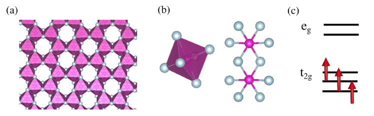
Figure 1: (a) Crystalline structure of CrI₃, showing the honeycomb arrangement of the chromium atoms. Every chromium atom has an octahedral iodine environment, where different octahedra are linked by an iodine forming an angle close to 90 degrees (b). The octahedral environment splits the d levels in the eg and t_2g manifolds (c). First Hund rule favors the $S=3/2$ state, with 3 fully polarized electrons in the $t_{2g}$ manifold.

Both experimental results McGuire et al. (2015); Huang et al. (2017) and DFT calculationsZhang et al. (2015); Wang et al. (2016b) show that CrI₃ is an semiconducting material with a the band-gap of $1.2$ eV.Dillon Jr and Olson (1965) In a single layer of CrI₃, the plane of Cr atoms form a honeycomb lattice and is sandwiched between two atomic planes of I. The Cr ions are surrounded by 6 first neighbor I atoms arranged in a corner sharing octahedra. In an ionic picture, the oxidation state of Cr in this compound is expected to be $+3$, with an electronic configuration $3s^{0}3d^{3}$. In an octahedral environment the $d$ levels split into a higher energy $e_{g}$ doublet and a lower energy $t_{2g}$ triplet.Abragam and Bleaney (2012) Thus, we expect that Cr³⁺ ions in this environment have $S=3/2$, with 3 electrons occupying the $t_{2g}$ manifold, complying with first Hund rule (see Fig (1)c. The lack of orbital degeneracy results in an orbital singletAbragam and Bleaney (2012) with a quenched orbital moment. This picture is consistent with the observedMcGuire et al. (2015) saturation magnetization of bulk CrI₃, that yields a magnetic moment of $\simeq$ 3$\mu_{B}$ per Cr atom, that can be explained with $S=3/2$ and $L=0$.

Single ion magnetic anisotropy is originated by the interplay of spin orbit coupling and the crystal field. In magnetic ions with a finite orbital moment, magnetic anisotropy scales like ${\cal E}_{\rm MAE}\propto\lambda\langle\vec{L}\rangle\cdot\langle\vec{S}\rangle$, where $\lambda$ is the magnetic ion atomic spin orbit coupling. However, when the orbital moment is quenched ($\langle\vec{L}\rangle=0$), this lowest order non-zero contribution arises from quantum fluctuations of the orbital moment, and is given by ${\cal E}_{\rm MAE}\propto\frac{\lambda^{2}}{\Delta}$, where $\Delta$ is the energy separation with the crystal field excited states of the ion. Given that $\lambda\simeq$ 10 meV for Cr,Kramida et al. (2015) and $\Delta$ is in the range of $500$ meV, single ion anisotropy energies are very often way below 1 meV. In a purely octahedral environment this quadratic contribution would actually vanish,Abragam and Bleaney (2012); Ferrón et al. (2015) and the magnetic anisotropy energy would scale like ${\cal E}_{\rm MAE}\propto\frac{\lambda^{4}}{\Delta^{3}}$, resulting in an extremely small single ion anisotropy. Based on these considerations, single ion anisotropy of Cr³⁺ in CrI₃ should arise from the distortion of the octahedral environment.

Magnetic interactions between magnetic ions separated by non-magnetic ligands arise via the super-exchange mechanism proposed by P. W. Anderson.Anderson (1950) This involves the virtual excitation of excited states where charge is transferred, during a Heisenberg time, from the ligand to the magnetic cations. This virtual processes reduce the total energy of the system and depend on the relative spin orientation of the magnetic atoms. The sign of this exchange interaction depends both on the angle $\theta$ formed by the two chemical bonds connecting the ligand and the magnetic atoms and on the filling of the $d$ levels of the cations. A set of rules to predict the sign of the interactions was proposed, independently, by J. B. GoodenoughGoodenough (1958) and Kanamori.Kanamori (1959) In particular, ferromagnetic interactions are maximal when the $\theta=90^{o}$. For CrI₃, the angle $\theta\simeq 93^{o}$, which accountsFeldkemper and Weber (1998) for the ferromagnetic interactions. As long as spin-orbit interactions are neglected, these exchange interactions are always spin rotational invariant and can be described with a Heisenberg coupling $J\vec{S}_{1}\cdot\vec{S}_{2}$.

The possibility of magnetic anisotropy in the superexchange interactions in magnetic insulators was proposed early on by T. Moriya.Moriya (1960) In his seminar work, he considered the anisotropic interactions originated by spin-orbit coupling in the magnetic ions. He found two types of addition to the Heisenberg coupling. The first are the Dzyaloshinski-Moriya (DM) term or antisymmetric exchange, $\vec{D}_{ij}\cdot\left(\vec{S}_{i}\times\vec{S}_{j}\right)$, postulated by Dzyaloshinski.Dzyaloshinsky (1958) The second is the anisotropic symmetric exchange, $\lambda S^{z}_{i}S^{z}_{j}$.

In the case of exchange mediated by an anion, the DM vector can be written asKeffer (1962) $\vec{D}_{ij}=\vec{r}_{i}\times\vec{r}_{j}$, where $\vec{r}_{i},\vec{r}_{j}$ link the anion with the two magnetic atoms. The DM favors non-collinear ground states. However, this term is absent in the CrI₃ crystal, since the two paths mediated by iodine contribute to with a DM vector with opposite sign that yield a net zero contribution. In contrast, the anisotropic symmetric exchange term is allowed by symmetry and, as we show below, it is definitely important in CrI₃. The symmetric and antisymmetric contributions to the anisotropic superexchange scale with $\lambda_{I}^{2}$ and $\lambda$, respectively,Moriya (1960) where $\lambda_{I}\simeq 0.6$eV, is the atomic spin orbit coupling of iodine.Kramida et al. (2015)

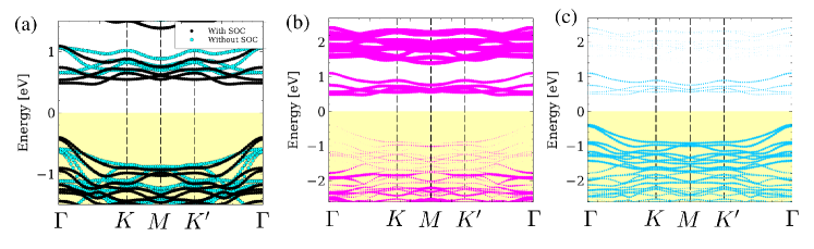
Figure 2: (a) Band structure of the system in the ferromagnetic state, without SOC (light blue) and with SOC (black). The large variation upon switching on spin orbit coupling cannot be accounted by the energy scale of the spin orbit coupling of chromium. Projection of the band structure over the chromium (b) and iodine (c) atoms. From panels (b,c) is inferred that the valence band shows a strong iodine character and that the conduction band is dominant from chromium, but with a non zero contribution from iodine. This chromium-iodine mixing is the responsible of the large variation of the conduction band upon switching on SOC, and is the ultimate responsible of the anisotropic exchange.

II Density functional methods

We perform density functional theory calculations with the pseudo-potential code Quantum EspressoGiannozzi et al. (2009) and the all-electron code ElkElk . Monolayer structures were relaxed with Quantum Espresso, Projector augmented wave (PAW) pseudopotentialsBlöchl (1994); Kucukbenli et al. (2014) and PBE exchange correlation functionalPerdew et al. (1996) in the ferromagnetic configuration. With the relaxed structures, calculation with Elk are carried out using spin orbit coupling in the non-collinear formalism, DFT+U with the Yukawa schemeBultmark et al. (2009) ($J=0.7$ eV and $U=2.7$ eV) in the fully localized limit and LDA exchange correlation functional.Perdew and Zunger (1981) We have verified that exchange energies with LDA or GGA, with or without DFT+U give qualitatively similar results.

The calculations of magnetic anisotropy require careful convergence of the total energy. We found that converging the total energy $10^{-8}$ eV yields stable results. We have used the feature of Elk that permits to tune the overall strength of spin orbit interaction by a dimensionless constant scale factor, that we call $\alpha$. Thus, for $\alpha>1$ the size of the spin orbit coupling is increased above its actual value. In addition, we have introduced a modification in the source code of Elk in order to selectively turn on and off the spin orbit coupling in the two different atoms independently, so that we now have two dimensionless scale factors, $\alpha_{I}$ and $\alpha_{Cr}$. As we discuss below, these two resources permit to to trace the origin of the magnetic anisotropy, as we discuss now.

III Electronic properties of CrI₃

We now describe the most salient electronic properties of CrI₃, as described within our DFT calculations, in line with previous workZhang et al. (2015); Liu et al. (2016). The calculations show that CrI₃ is a ferromagnetic semiconductor. The magnetic moment resides mostly in the Cr atoms, with a residual counterpolarized magnetization on the $I$ atoms. The total magnetic moment in the unit cell is 6 $\mu_{B}$, 3$\mu_{B}$ per Cr atom. Figure 2a shows the band structure, calculated with and without SOC. The bands undergo a rather large shift, in the range of $0.1$ eV, when SOC is included,. The size of this shift is a first indication that the spin orbit interaction of iodine atoms plays an important role,Wu et al. (2012) as spin orbit coupling in Cr is much smaller than $0.1$ eV. Figure 2b,c shows the bands weighted over the projection on the $d$ orbitals of Cr (Fig. 2b) and the $p$ orbitals of I (Fig. 2c). It is apparent that the top of the valence band is formed mostly by spin unpolarized $p$ orbitals of the I atoms, and the conduction band is formed by $d$ orbitals of Cr. The lowest lying states of the conduction band are majority $e_{g}$ orbitals, (around 0.7 eV in Fig. 2) whereas the minority states are located at higher energies (around 2 eV in Fig. 2). The majority spin $d$ orbitals, of the $t_{2g}$ manifold, are found $2$ eV below the top of the valence bands. The shape of the magnetization field, not shown, clearly shows that the magnetic moment resides in orbitals with $t_{2g}$ symmetry, in line with previous results.Liu et al. (2016)

IV Magnetic anisotropy

We are now in position to discuss the main topic of this work, magnetic anisotropy. We have verified that the in-plane anisotropy is negligibly small. Therefore, in the following we focus on the off-plane anisotropy and we compute the quantity:

$${\cal E}_{\rm MAE}=E_{G}(0)-E_{G}(90)$$ (1)

where $E_{G}(\theta)$ is the computed ground state energy as a function of the angle $\theta$ that forms the magnetic moment with the atomic planes. ${\cal E}_{\rm MAE}>0$ describes an off-plane easy axis system. For the in-plane component, we take $M_{y}=0$. In line with previous work,Zhang et al. (2015) we obtain ${\cal E}_{\rm MAE}=0.65$ meV. Thus, the calculation predicts that the system has an easy axis anisotropy, perpendicular to the atomic planes, in agreement with the experiments.Huang et al. (2017)

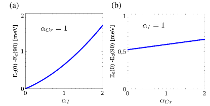
Figure 3: (a) Evolution of the magnetic anisotropy energy as a function of the spin-orbit coupling in iodine $\alpha_{I}$, keeping the spin-orbit coupling in Cr to the real value $\alpha_{Cr}=1$ (b) Same, reverting the roles of I and Cr. These curves show the dominant contribution of iodine spin orbit coupling to the MAE.

In order to study the origin of this magnetic anisotropy we compute how ${\cal E}_{\rm MAE}$ changes as we vary independently spin orbit coupling in two atoms.Kośmider et al. (2013) To do so, here we define the DFT Hamiltonian as

$${\cal H}_{\rm DFT}(\alpha_{I},\alpha_{Cr})={\cal H}_{0}+\alpha_{I}{\cal H}^{SOC}_{I}+\alpha_{Cr}{\cal H}^{SOC}_{Cr}$$ (2)

where $\mathcal{H}_{0}$ is the non relativistic Hamiltonian, $\mathcal{H}_{Cr}$ the relativistic Hamiltonian correction to chromium and $\mathcal{H}_{I}$ the relativistic Hamiltonian correction to iodine. We compute magnetic anisotropy energy from Eq. 1, keeping at the default value $\alpha_{Cr,I}=1$ only one of the species, and ramping the other. The results are shown in Figs. 3a,b and permit to conclude that MAE arises predominantly from the spin orbit coupling in iodine atoms. This suggests that anisotropic symmetric superexchange is the likely cause of magnetic anisotropy in this compound. This also seems to indicate that the local moments do not have a strong single ion anisotropy, and therefore they are not properly described as Ising spins.

IV.1 Spin Hamiltonian

In order to validate these hypothesis, we now propose a model Hamiltonian for the spins of the Cr atoms in the honeycomb lattice:

$${\cal H}=-\left(\sum_{i}D(S^{z}_{i})^{2}+\frac{J}{2}\sum_{i,i^{\prime}}\vec{S}_{i}\cdot\vec{S}_{i^{\prime}}+\frac{\lambda}{2}\sum_{i,i^{\prime}}S^{z}_{i}S^{z}_{i^{\prime}}\right)$$ (3)

where the sum over $i$ runs over the entire lattice of Cr atoms, and the sum over $i^{\prime}$ runs over the 3 atoms, the first neighbors of atom $i$. The first term in the Hamiltonian describes the easy axis single ion anisotropy and we choose $z$ as the off-plane direction. The second term is the Heisenberg isotropic exchange and the final term is the anisotropic symmetric exchange. The sign convention is such that $J>0$ favors ferromagnetic interactions and $D>0$ favors off-plane easy axis. $\lambda=0$ would imply a completely isotropic exchange interaction.

We first treat Eq. 3 in the classical approximation, and we describe the spins $\vec{S}$ as dimensionless classical vectors of length $S$ in the sphere We write the energy of the ground state for 4 possible ground states, depicted in Fig. 4a: (I) ferromagnetic off-plane (FM,z) , (II) antiferromagnetic off-plane (AF,z), (III) ferromagnetic in-plane (FM,x) and (IV) antiferromagnetic in-plane (AF,x). We denote the corresponding classical ground state energies as ${\cal E}_{FM,z},{\cal E}_{AF,z},{\cal E}_{FM,x},{\cal E}_{AF,x}$. The spin model allows to write the energetics of the different configurations normalized per unit cell (2 Cr atoms) as

$${\cal E}_{FM,z}=-2S^{2}D-3S^{2}(J+\lambda)$$ (4)

$${\cal E}_{AF,z}=-2S^{2}D+3S^{2}(J+\lambda)$$ (5)

$${\cal E}_{FM,x}=-3S^{2}J$$ (6)

$${\cal E}_{AF,x}=+3S^{2}J$$ (7)

with $S=3/2$ for CrI₃. In order to determine $J$, $D$ and $\lambda$, we use the ground state energies for these 4 configurations as obtained from our DFT calculations. In addition, we do this ramping the overall strength of the spin orbit coupling, $\alpha=\alpha_{Cr}=\alpha_{I}$. For $\alpha=1$ we obtain $J=2.2$ meV, in line with the results by Zhang et al.Zhang et al. (2015) Our results for $D$ and $\lambda$ are shown in Fig. 4b. It is apparent that the anisotropic symmetric exchange $\lambda$ is much bigger than the single ion anisotropy $D$, in particular for $\alpha=1$. The precise value of $D$ was affected by numerical noise in the regime where both $J$ and $\lambda$ already reached convergence, being always $D$ at least 30 times smaller that the anisotropic exchange $\lambda$. This yields a value of D negligible with respect any other exchange energy scale. Thus, we have $J>\lambda>>D$, which lead us to claim that the adequate spin model for CrI₃ is the XXZ model with negligible single ion anisotropy. This is the most important result of this work. We find $\lambda=0.04J=0.09$ meV for $\alpha=1$. Thus, the flip-flop exchange is just 4 percent smaller than the Ising exchange $S^{z}_{i}S^{z}_{j}$, given by $J+\lambda$. Whereas the spin-flip part of exchange is actually responsible of the existence of dispersive spin wave excitations, the anisotropic term $\lambda$ opens up a gap in their spectrum, as we show below. This actually controls the transition from the ferromagnetic to the non-magnetic phase as the material is heated above $T_{c}$:

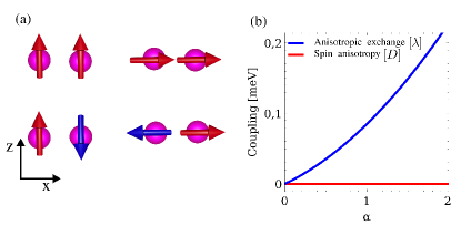
Figure 4: (a) Sketch and energetics of the different collinear magnetic configurations for two chromium atoms, showing in-plane and off-plane ferromagnetic and antiferromagnetic configurations. Comparison with DFT permits to extract $J$, $D$ and $\lambda$ (see text). (b) Evolution of the single ion anisotropy $D$ and anisotropic exchange $\lambda$ as a function of the spin orbit coupling $\alpha$, where $\alpha=1$ corresponds to the real value, as described at the DFT level.

V Spin Wave theory

We now go beyond the classical approximation used in the previous section. To do that, we now treat the spins in Hamiltonian (3) as quantum mechanical $S=3/2$ operators. We treat the Hamiltonian within the linear spin wave approximation. To do so, we use the so called Holstein-Primakoff representation Holstein and Primakoff (1940) of the spin operators in terms of bosonic operators

$$S^{+}_{i}=\sqrt{2S}\sqrt{1-\frac{b_{i}^{\dagger}b_{i}}{2S}}b_{i}$$ (8)

$$S^{-}_{i}=\sqrt{2S}b_{i}^{\dagger}\sqrt{1-\frac{b_{i}^{\dagger}b_{i}}{2S}}$$ (9)

$$S^{z}_{i}=S-b_{i}^{\dagger}b_{i}$$ (10)

with $b_{i}$ and $b^{\dagger}_{i}$ the bosonic annihilation and creation operator in site. The representation of the spin Hamiltonian (3) in terms of this bosonic operators leads a complicated non-linear Hamiltonian. The spin wave approximation consist in keeping only the quadratic terms in the bosonic operators $b$. This approximation is valid for a small occupation of the bosonic modes, ie, when the magnetization is closed to $S_{z}\simeq S$, ie, for small temperatures. In the spin wave approximation, the effective Hamiltonian for the spin excitations reads:

$$\mathcal{H}_{\rm spin\,waves}=\sum_{i}\left(2DS+3S(J+\lambda)\right)b^{\dagger}_{i}b_{i}-JS\sum_{\langle ij\rangle}b^{\dagger}_{i}b_{j}$$ (11)

where the sum over $i$ runs over the entire lattice and the sum over $j$ runs over the first neighbors of $j$. This Hamiltonian describes bosonic excitations moving in a honeycomb lattice, with an on-site energy $\epsilon_{0}=2DS+3S(J+\lambda)$ and a hopping energy $JS$. Thus, the Bloch Hamiltonian for the honeycomb lattice reads

$${\cal H}_{SW}(\vec{k})=\left(\begin{array}[]{cc}\epsilon_{0}&-JSf(\vec{k})\\ -JSf^{*}(\vec{k})&\epsilon_{0}\end{array}\right)$$ (14)

where $\epsilon_{0}=3JS+2SD+3S\lambda$, $f(\vec{k})=1+e^{i\vec{k}\cdot\hat{a}_{1}}+e^{i\vec{k}\cdot\hat{a}_{2}}$ is the usual form factor for the honeycomb lattice, and $\hat{a}_{1,2}$ are the unit vectors of the triangular lattice. The resulting energy spectrum is

$$E^{\pm}(\vec{k})=\epsilon_{0}\pm JS\sqrt{|f(\vec{k}|^{2}}$$ (15)

We can expand the lower band around its minima at the $\Gamma$ point, to get

$$E^{-}(\vec{k})\simeq\Delta_{0}+\rho k^{2}$$ (16)

where the spin wave gap is given by

$$\Delta_{0}=2DS+3S\lambda$$ (17)

For CrI₃ we can take $D=0$ and we have a spin wave gap $\Delta_{0}=3S\lambda=0.4$ meV. The so called spin stiffness is given by

$$\rho=\frac{1}{4}JS$$ (18)

that yields for CrI₃ a value $\rho=0.82$ meV. The ratio $\frac{\Delta_{0}}{\rho}=\frac{12\lambda}{J}\simeq 0.49$ plays an important role in the following.

From Eqs. 16,17 it is apparent that if the two terms that break spin rotational invariance in the original Hamiltonian (3), $D$ and $\lambda$, vanish, the spin wave spectrum becomes gapless. Therefore, in the spin wave spectrum, both the anisotropic exchange and the single ion anisotropy create a gap in the spin waves (see Fig. 5a), so that their effect on the spin wave dispersion is similar. This implies that simple inspection of the spin wave dispersion does not provide enough information to asses whether if the correct model for a compound is single ion anisotropy or anisotropic exchange, and input from a microscopic first principles calculation is necessary. As we discuss now, the presence of their induced gap is essential to have magnetization at finite temperature.

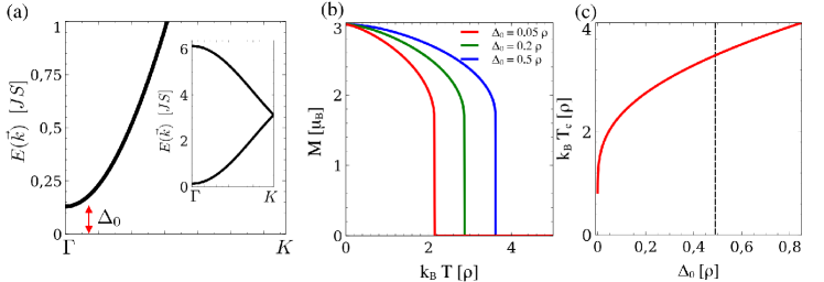
Figure 5: (a) Example of the spin wave dispersion, showing a gap in the spin excitations. (b) Selfconsistent solution of the magnetization derived with Eq. 27, showing a depleted magnetization with increasing temperature. (c) Numerical solution for the critical temperature as a function of the spin wave gap $\Delta_{0}$, showing a logarithmic dependence on $\Delta_{0}$. The dashed line in (c) is the result obtained for CrI₃ with the DFT calculations.

V.1 Low temperature magnetization

Every magnon carries one unit of angular momentum. Therefore, in the linear spin wave framework, we can approximate the magnetization by

$$M(T)=S-\delta M=S-\frac{1}{2(2\pi)^{2}}\int_{BZ}\frac{d^{2}\vec{k}}{e^{\beta E(\vec{k})}-1}$$ (19)

where $M(T)$ is the magnetization in units of $\hbar$ per Cr atom as a function of the temperature, the factor $1/2$ comes from having two Cr atoms in the unit cell and $\beta^{-1}=k_{B}T$. Linear spin wave theory works well when the magnon density is small. In the following we use the fact that this integral is controlled by the low energy magnons, and we approximate $E(\vec{k})$ by Eq. (16). In addition, we replace the integral over the Brillouin zone by the integral over a circle of radius $k_{c}$, chosen so that the density of magnons is properly normalized $\frac{1}{2\pi}\int_{0}^{k_{c}}kdk=2$. Choosing this normalization includes the contribution from the high energy magnon branch in the high energy part of the dispersion. We first focus in the case $\Delta_{0}=0$, i.e. in the absence of anisotropic exchange, in that case the correction of the magnetization goes as

$$\delta M=\frac{1}{4\pi}\int^{k_{c}}_{0}\frac{kdk}{\beta\rho k^{2}}\rightarrow\infty$$ (20)

This divergence signals the absence of order at finite temperature in the Heisenberg model in the gapless regime $\Delta_{0}=0$, consistent with the Mermin-Wagner theorem.Mermin and Wagner (1966) Therefore, the anisotropy gap is essential to protect the long range order in 2D.

We will move now to the case of finite spin wave gap $\Delta_{0}\neq 0$. We now consider the very low temperature case, $\beta\Delta_{0}>>1$. We can then approximateBruno (1991)

$$M(T)=M(T=0)+\delta M=S-\frac{k_{B}T}{2\pi JS}e^{-\Delta_{0}/k_{B}T}$$ (21)

Thus, we expect that the magnetization will have a very weak temperature dependence for temperatures smaller than spin wave gap. According to our calculations $\Delta_{0}=0.4$ meV, so $M(T)$ be almost maximal up to $T=5$ K.

V.2 Estimate of $T_{c}$

We now provide a rough estimate of the Curie temperature, based on non linear spin wave theory . We use the initial expression for spin operators, and expand them retaining the up to fourth order in the bosonic operators

$$S^{+}_{i}\approx\sqrt{2S}\left(1-\frac{b_{i}^{\dagger}b_{i}}{4S}\right)b_{i}$$ (22)

$$S^{-}_{i}\approx\sqrt{2S}b_{i}^{\dagger}\left(1-\frac{b_{i}^{\dagger}b_{i}}{4S}\right)$$ (23)

$$S^{z}_{i}=S-b_{i}^{\dagger}b_{i}$$ (24)

At intermediate temperatures, there is a finite number of spin waves, that is accounted by the higher order terms in bosonic operators when substituting the previous expansion in the spin Hamiltonian. In that situation, the spin Hamiltonian contains four field operators and therefore is not exactly solvable. Thus, the effect of the spin wave population is described using a mean field approximation in the spin wave Hamiltonian by means of the substitution $b_{i}^{\dagger}b_{i}b_{j}^{\dagger}b_{j}\approx\langle b_{i}^{\dagger}b_{i}\rangle b_{j}^{\dagger}b_{j}+b_{i}^{\dagger}b_{i}\langle b_{j}^{\dagger}b_{j}\rangle+\mathcal{C}$. With the previous approximation it is straightforward to check that a finite population of spin waves is equivalent to a renormalization of the hopping energy and spin wave gap asStanek et al. (2011)

$$JS\rightarrow J(S-\langle b^{\dagger}b\rangle)=JM(T)$$ (25)

$$\lambda S\rightarrow\lambda(S-\langle b^{\dagger}b\rangle)=\lambda M(T)$$ (26)

The previous substitutions lead to a selfconsistent equation for the magnetization as

$$M=S-\frac{1}{2(2\pi)^{2}}\int_{BZ}\frac{d^{2}\vec{k}}{e^{\beta ME(\vec{k})/S}-1}$$ (27)

where the integral extends over the first Brillouin zone. A qualitative behavior of the previous integral can be obtained approximating $E(\vec{k})=\Delta_{0}+\rho k^{2}$ and $e^{\beta\frac{M}{S}E(k)}-1\approx\beta M(\Delta_{0}+\rho k^{2})/S$. As Eq. (27) has no solution for $M=0$, we define $T_{c}$ as the temperature at which the magnetization is depleted to $M=S/2$. This leads to the following equation:

$$k_{B}T_{c}\simeq\frac{2\pi\rho S}{\log\frac{\Delta_{0}+8\pi\rho}{\Delta_{0}}}=\frac{\pi JS^{2}}{2\log\frac{\Delta_{0}+2\pi JS}{\Delta_{0}}}$$ (28)

A very similar result can be obtained using different spin representations.Irkhin et al. (1999); Grechnev et al. (2005) Equation (28), together with the numerical solutionBloch (1962) of Eq. (27) in Fig(5)b, show several important results. First, $T_{c}$ is an increasing function of the spin wave gap $\Delta_{0}$ (see Fig. (5c). This is in line with the experimental results recently reported for Cr₂Ge₂Te₆,Gong et al. (2017) for which the major contribution to the spin wave gap comes from the Zeeman contribution, due to the very tiny intrinsic anisotropy, resulting in dramatic variations of $T_{c}$ as a function of the applied field. This is a feature specific of two dimensional magnets with dispersive spin waves. Second, $T_{c}$ is significantly smaller than the prediction coming from the Ising model. The exact solution for the Ising model in the honeycomb latticeMeyer (2000) yields $k_{B}T_{c}=1.51j$, where $j$ is the coupling between classical spins with $S=1$. Using this result for CrI₃, we would have $k_{B}T_{c}=1.51(J+\lambda)S^{2}=85$ Kelvin, that overshoots the experimental value 45 K.

On the other hand, using the prediction of $T_{c}$ obtained by the numerical solution of Eq. (27) shown in Fig. 5c, we obtain a value of $k_{B}T_{c}=3.5\rho$, for $\Delta_{0}=0.49\rho$, that gives $T_{c}=33$ K, understimating the the experimental valueHuang et al. (2017) $T_{c}=45$ K by 20%. Including the effect of the finite magnetic field would increase $\Delta_{0}$, and push the prediction upward. Inclusion of longer range couplingSivadas et al. (2015); Foyevtsova et al. (2011); Jeschke et al. (2013); Foyevtsova et al. (2013) is also expected to increase the spin stiffness, yielding a larger estimate of the critical temperature. Furthermore, a more accurate treatment must consider the explicit spin wave density of states and a more careful treatment of fluctuations close to the critical point. The discrepancy highlights the limitations of the non-linear spin wave theory, and perhaps, also those of the DFT scheme to determine the energy scales of the Hamiltonian. Nevertheless, apart from the previous limitations, our approach highlights the role played by anisotropic exchange, as the ultimate mechanism responsible to controlling the divergence in Eq. 28.

VI Conclusions

We have studied the origin of magnetic anisotropy in two dimensional CrI₃, a recently discovered ferromagnetic two dimensional crystal with off-plane anisotropy. We have found that magnetic anisotropy in this system comes predominantly from the superexchange interaction, that gives rise to an anisotropic contribution to the conventional exchange interaction. The strength of the non Heisenberg correction is found to be controlled by the spin orbit coupling of the intermediate iodine atom. The single ion anisotropy of the magnetic Cr atoms is found to give a negligible contribution to magnetic anisotropy. The suppression of the single ion anisotropy due to the octahedral environment, together with large spin orbit coupling of iodine, make the anisotropic exchange the leading mechanism stabilizing the magnetic ordering in 2D CrI₃. Our calculations permit to conclude that the effective spin Hamiltonian for CrI₃ is a XXZ model. In turn, this implies that gapped spin waves are the essential elementary excitations that control the finite temperature properties of this new type of magnetic system. Given that spin waves in two dimensions are interesting on its own right, as they can exhibit thermal Hall effect and have topologically non-trivial phases.Hirschberger et al. (2015); Chisnell et al. (2015); Roldán-Molina et al. (2016); Owerre (2016); Zyuzin and Kovalev (2016); Cheng et al. (2016) As an example, one can consider inducing a Dzyaloshinskii-Moriya term in a CrI₃ monolayer by applying a perpendicular electric field, opening the possibility of a skyrmionic ground state whose magnonic Hamiltonian is topologically non-trivial and shows gapless edge magnonic excitations.Roldán-Molina et al. (2016) Another interesting playground would be the possibility of applying non uniform strain to the ferromagnetic monolayer, modulating the exchange constants and creating an artificial gauge field in the magnonic Hamiltonian.Kraus and Zilberberg (2016); Kraus et al. (2013) Therefore, the discovery of magnetic 2D crystals paves the way towards the exploration of these exciting phenomena.

References

- Gong et al. (2017) C. Gong, L. Li, Z. Li, H. Ji, A. Stern, Y. Xia, T. Cao, W. Bao, C. Wang, Y. Wang, Z. Q. Qiu, R. J. Cava, S. G. Louie, J. Xia, and X. Zhang, Nature 546, 265 (2017).
- Huang et al. (2017) B. Huang, G. Clark, E. Navarro-Moratalla, D. R. Klein, R. Cheng, K. L. Seyler, D. Zhong, E. Schmidgall, M. A. McGuire, D. H. Cobden, W. Yao, D. Xiao, P. Jarillo-Herrero, and X. Xu, Nature 546, 270 (2017).
- Wang et al. (2016a) X. Wang, K. Du, Y. Y. F. Liu, P. Hu, J. Zhang, Q. Zhang, M. H. S. Owen, X. Lu, C. K. Gan, P. Sengupta, et al., 2D Materials 3, 031009 (2016a).
- Lee et al. (2016) J.-U. Lee, S. Lee, J. H. Ryoo, S. Kang, T. Y. Kim, P. Kim, C.-H. Park, J.-G. Park, and H. Cheong, Nano Letters 16, 7433 (2016).
- Lu et al. (2015) J. Lu, O. Zheliuk, I. Leermakers, N. F. Yuan, U. Zeitler, K. T. Law, and J. Ye, Science 350, 1353 (2015).
- Ugeda et al. (2016) M. M. Ugeda, A. J. Bradley, Y. Zhang, S. Onishi, Y. Chen, W. Ruan, C. Ojeda-Aristizabal, H. Ryu, M. T. Edmonds, H.-Z. Tsai, et al., Nature Physics 12, 92 (2016).
- Xi et al. (2015) X. Xi, L. Zhao, Z. Wang, H. Berger, L. Forró, J. Shan, and K. F. Mak, Nature nanotechnology 10, 765 (2015).
- Chang et al. (2016) K. Chang, J. Liu, H. Lin, N. Wang, K. Zhao, A. Zhang, F. Jin, Y. Zhong, X. Hu, W. Duan, et al., Science 353, 274 (2016).
- Ma et al. (2012) Y. Ma, Y. Dai, M. Guo, C. Niu, Y. Zhu, and B. Huang, ACS nano 6, 1695 (2012).
- Sachs et al. (2013) B. Sachs, T. O. Wehling, K. S. Novoselov, A. I. Lichtenstein, and M. I. Katsnelson, Phys. Rev. B 88, 201402 (2013).
- Chittari et al. (2016) B. L. Chittari, Y. Park, D. Lee, M. Han, A. H. MacDonald, E. Hwang, and J. Jung, Physical Review B 94, 184428 (2016).
- Geim and Grigorieva (2013) A. K. Geim and I. V. Grigorieva, Nature 499, 419 (2013).
- Zhong et al. (2017) D. Zhong, K. L. Seyler, X. Linpeng, R. Cheng, N. Sivadas, B. Huang, E. Schmidgall, T. Taniguchi, K. Watanabe, M. A. McGuire, et al., Science Advances 3, e1603113 (2017).
- Mermin and Wagner (1966) N. D. Mermin and H. Wagner, Phys. Rev. Lett. 17, 1133 (1966).
- Onsager (1944) L. Onsager, Phys. Rev. 65, 117 (1944).
- Rau et al. (2014) I. G. Rau, S. Baumann, S. Rusponi, F. Donati, S. Stepanow, L. Gragnaniello, J. Dreiser, C. Piamonteze, F. Nolting, S. Gangopadhyay, et al., Science 344, 988 (2014).
- Jensen and Mackintosh (1991) J. Jensen and A. R. Mackintosh, Rare earth magnetism (Clarendon Oxford, 1991).
- Dillon Jr and Olson (1965) J. Dillon Jr and C. Olson, Journal of Applied Physics 36, 1259 (1965).
- McGuire et al. (2015) M. A. McGuire, H. Dixit, V. R. Cooper, and B. C. Sales, Chemistry of Materials 27, 612 (2015).
- Zhang et al. (2015) W.-B. Zhang, Q. Qu, P. Zhu, and C.-H. Lam, Journal of Materials Chemistry C 3, 12457 (2015).
- Wang et al. (2016b) H. Wang, F. Fan, S. Zhu, and H. Wu, EPL (Europhysics Letters) 114, 47001 (2016b).
- Abragam and Bleaney (2012) A. Abragam and B. Bleaney, Electron paramagnetic resonance of transition ions (OUP Oxford, 2012).
- Kramida et al. (2015) A. Kramida, Yu. Ralchenko, J. Reader, and and NIST ASD Team, NIST Atomic Spectra Database (ver. 5.3), [Online]. Available: http://physics.nist.gov/asd [2017, April 12]. National Institute of Standards and Technology, Gaithersburg, MD. (2015).
- Ferrón et al. (2015) A. Ferrón, F. Delgado, and J. Fernández-Rossier, New Journal of Physics 17, 033020 (2015).
- Anderson (1950) P. Anderson, Physical Review 79, 350 (1950).
- Goodenough (1958) J. B. Goodenough, Journal of Physics and Chemistry of Solids 6, 287 (1958).
- Kanamori (1959) J. Kanamori, Journal of Physics and Chemistry of Solids 10, 87 (1959).
- Feldkemper and Weber (1998) S. Feldkemper and W. Weber, Phys. Rev. B 57, 7755 (1998).
- Moriya (1960) T. Moriya, Phys. Rev. 120, 91 (1960).
- Dzyaloshinsky (1958) I. Dzyaloshinsky, Journal of Physics and Chemistry of Solids 4, 241 (1958).
- Keffer (1962) F. Keffer, Phys. Rev. 126, 896 (1962).
- Giannozzi et al. (2009) P. Giannozzi, S. Baroni, N. Bonini, M. Calandra, R. Car, C. Cavazzoni, D. Ceresoli, G. L. Chiarotti, M. Cococcioni, I. Dabo, A. Dal Corso, S. de Gironcoli, S. Fabris, G. Fratesi, R. Gebauer, U. Gerstmann, C. Gougoussis, A. Kokalj, M. Lazzeri, L. Martin-Samos, N. Marzari, F. Mauri, R. Mazzarello, S. Paolini, A. Pasquarello, L. Paulatto, C. Sbraccia, S. Scandolo, G. Sclauzero, A. P. Seitsonen, A. Smogunov, P. Umari, and R. M. Wentzcovitch, Journal of Physics: Condensed Matter 21, 395502 (19pp) (2009).
- (33) “Elk code, http://elk.sourceforge.net/,” .
- Blöchl (1994) P. E. Blöchl, Phys. Rev. B 50, 17953 (1994).
- Kucukbenli et al. (2014) E. Kucukbenli, M. Monni, B. Adetunji, X. Ge, G. Adebayo, N. Marzari, S. De Gironcoli, and A. D. Corso, arXiv preprint arXiv:1404.3015 (2014).
- Perdew et al. (1996) J. P. Perdew, K. Burke, and M. Ernzerhof, Phys. Rev. Lett. 77, 3865 (1996).
- Bultmark et al. (2009) F. Bultmark, F. Cricchio, O. Grånäs, and L. Nordström, Phys. Rev. B 80, 035121 (2009).
- Perdew and Zunger (1981) J. P. Perdew and A. Zunger, Phys. Rev. B 23, 5048 (1981).
- Liu et al. (2016) J. Liu, Q. Sun, Y. Kawazoe, and P. Jena, Physical Chemistry Chemical Physics 18, 8777 (2016).
- Wu et al. (2012) X. Wu, Y. Cai, Q. Xie, H. Weng, H. Fan, and J. Hu, Phys. Rev. B 86, 134413 (2012).
- Note (1) In the case , the weight of the orbitals at the top of the valence band increases.
- Kośmider et al. (2013) K. Kośmider, J. W. González, and J. Fernández-Rossier, Phys. Rev. B 88, 245436 (2013).
- Holstein and Primakoff (1940) T. Holstein and H. Primakoff, Physical Review 58, 1098 (1940).
- Bruno (1991) P. Bruno, Phys. Rev. B 43, 6015 (1991).
- Stanek et al. (2011) D. Stanek, O. P. Sushkov, and G. S. Uhrig, Phys. Rev. B 84, 064505 (2011).
- Irkhin et al. (1999) V. Y. Irkhin, A. Katanin, and M. Katsnelson, Physical Review B 60, 1082 (1999).
- Grechnev et al. (2005) A. Grechnev, V. Y. Irkhin, M. I. Katsnelson, and O. Eriksson, Physical Review B 71, 024427 (2005).
- Bloch (1962) M. Bloch, Phys. Rev. Lett. 9, 286 (1962).
- Meyer (2000) P. Meyer, School of Mathematics and Computing, University of Derby (2000).
- Sivadas et al. (2015) N. Sivadas, M. W. Daniels, R. H. Swendsen, S. Okamoto, and D. Xiao, Phys. Rev. B 91, 235425 (2015).
- Foyevtsova et al. (2011) K. Foyevtsova, I. Opahle, Y.-Z. Zhang, H. O. Jeschke, and R. Valentí, Phys. Rev. B 83, 125126 (2011).
- Jeschke et al. (2013) H. O. Jeschke, F. Salvat-Pujol, and R. Valentí, Phys. Rev. B 88, 075106 (2013).
- Foyevtsova et al. (2013) K. Foyevtsova, H. O. Jeschke, I. I. Mazin, D. I. Khomskii, and R. Valentí, Phys. Rev. B 88, 035107 (2013).
- Hirschberger et al. (2015) M. Hirschberger, R. Chisnell, Y. S. Lee, and N. P. Ong, Phys. Rev. Lett. 115, 106603 (2015).
- Chisnell et al. (2015) R. Chisnell, J. S. Helton, D. E. Freedman, D. K. Singh, R. I. Bewley, D. G. Nocera, and Y. S. Lee, Phys. Rev. Lett. 115, 147201 (2015).
- Roldán-Molina et al. (2016) A. Roldán-Molina, A. Nunez, and J. Fernández-Rossier, New Journal of Physics 18, 045015 (2016).
- Owerre (2016) S. Owerre, Journal of Applied Physics 120, 043903 (2016).
- Zyuzin and Kovalev (2016) V. A. Zyuzin and A. A. Kovalev, Phys. Rev. Lett. 117, 217203 (2016).
- Cheng et al. (2016) R. Cheng, S. Okamoto, and D. Xiao, Phys. Rev. Lett. 117, 217202 (2016).
- Kraus and Zilberberg (2016) Y. E. Kraus and O. Zilberberg, Nature Physics 12, 624 (2016).
- Kraus et al. (2013) Y. E. Kraus, Z. Ringel, and O. Zilberberg, Phys. Rev. Lett. 111, 226401 (2013).