Hydrodynamic stability in the presence of a stochastic forcing: a case study in convection
Abstract
We investigate the stability of statistically stationary conductive states for Rayleigh-Bénard convection that arise due to a bulk stochastic internal heating. Our results indicate that stochastic forcing at small magnitude has little to no effect, while strong stochastic forcing has a destabilizing effect. The methodology put forth in this article, which combines rigorous analysis with careful computation, provides an approach to hydrodynamic stability which is applicable to a variety of systems subject to a large scale stochastic forcing.
keywords:
1 Introduction
Rayleigh Bénard convection, the buoyancy driven motion of a fluid under the influence of a gravitational field, is ubiquitous in nature. It is one of the driving forces in a variety of situations ranging from boiling a pot of water, to geophysical processes, to pattern formation in stellar dynamics. Yet, despite remarkable advances in mathematical, computational, and experimental analysis, fundamental aspects of Rayleigh-Bénard convection remain poorly understood [1, 2].
The seminal work of Lord Rayleigh [3], inspired by the experiments of Bénard [4], quantified the onset of convection in terms of the instability of purely conductive solutions of the Boussinesq equations. In [3] it is established that when the Rayleigh number (a dimensionless parameter proportional to the boundary heating) is less than a critical value , then the purely conductive state is globally attractive. Not only did [3] place the study of thermal convection on a firm mathematical basis, but this work also yielded a now canonical example in the study of hydrodynamic stability [5].
Various modifications to Rayleigh’s original model, including alternative boundary conditions and different sources of heat (see [6] for example) have been considered in the past century. A natural further extension is to define and quantify stability for convective flows driven by stochastic forcing as many heat sources (as well as other sources of buoyancy instability) are inherently noisy. For example, radioactive decay in the earth’s mantle and thermonuclear reactions in large stars are inherently stochastic, see [7, 8].
Here we investigate the hydrodynamic stability of a conductive state for a stochastic variation to the standard Rayleigh-Bénard convection model, when an internal bulk stochastic source is present. Our approach relies on a combination of energy stability methods, ergodic theory, and numerical computation. It is notable that the methodology developed in this work applies to a larger class of randomly forced hydrodynamic systems which we will address in future studies. The current investigation is also closely related to previous research by the authors on the ergodic theory and dynamical properties of stochastically driven models for Rayleigh-Bénard convection ([9, 10, 11]). Throughout the following, we provide some rigorous justification of arguments and calculations leading to our final stability result.
While this investigation is new to the best of our knowledge, significant previous efforts have been made to incorporate random perturbations into models of convection. To understand the influence of thermal fluctuations, in [12, 13, 14, 15] the Boussinesq system modulated by singular (that is, active at all spatial frequencies) small noise in the bulk is investigated, and a reduced model is derived to describe flow statistics. This model leads to accurate predictions of the rate of heat transfer near the onset of convection ([16]), but requires stochastic forcing stronger than the predicted thermal fluctuations. We emphasize that these efforts were motivated by experimental observations, and the modeled noise was initiated in an effort to determine the potential influence of thermal fluctuations on carefully calibrated experiments.
One significant difficulty in the approach initiated in [13] is that the presence of a generic stochastic source eliminates the existence of a traditionally defined conductive state for which the velocity field is zero, see [12, 13, 14, 17, 16, 15] and containing references for relevant details. The current investigation is not to ascertain the effect of thermal fluctuations on the onset of convection, but rather to determine the influence of stochastic effects that appear on the scale of the full system. The goal of this investigation is to extend and further quantify a setting similar to that proposed in [18] which considered the 2-dimensional Boussinesq equations with stochastic horizontal boundary conditions, and identified a substitute “quasi-conductive regime”, for which the velocity of solutions is non-zero but small. In [18] the authors numerically showed that these quasi-conductive states maintain stability for a wide range of Rayleigh numbers containing the classical critical value .
The current investigation will extend the results of [18] to a setting where the noise is physically motivated, yet difficult if not impossible to imitate in the laboratory implying that the asymptotic and numerical investigation detailed below is necessary. [13] and the studies that followed addressed concerns raised by thermal fluctuations in an experimental setting. The current study is instead motivated by noise that occurs on a larger scale that is not observed experimentally, but is relevant in a practical setting as discussed below. As such, we will not compare the results with experimental data, but infer that the instabilities suggested by the current analysis are relevant in nature and engineering applications. Essentially the goal of this study is to evaluate the impact that a dominating, large-scale noise will have on the stability of the determined conductive state, a situation that is not realized to our knowledge in any current experimental investigation.
The numerical stability results and their rigorous justification detailed below complement the theoretical development of rigorous ergodic theorems for stochastically forced Navier-Stokes equations, and related systems. For example, [19, 20] have established that the periodic 2-dimensional Navier-Stokes equations with a bulk stochastic forcing possesses a unique ergodic invariant measure provided the stochastically forced modes satisfy a modest geometric constraint. These results have been extended to the stochastic Boussinesq equations by the authors with various boundary conditions and parameter constraints ([9, 10, 11]). In these settings, the unique invariant measure is almost surely globally attractive in a statistical sense. In contrast when the stochastic forcing is “more degenerate”, that is, when the noise is horizontally stratified then the long-time stability of statistics is much less clear when the Rayleigh number is large. A discussion of this setting is the main goal of the present manuscript.
The starting point of the current investigation is the observation that, for certain classes of horizontally stratified volumetric forcing the system admits a dynamically inactive, conductive state . This conductive solution has an explicit form and admits Gaussian statistics whose mean and covariance are readily determined. Our primary goal in the following is to investigate the onset of convection as a bifurcation from this conductive state.
Note that our setup thus contrasts from the approach to onset taken in [13, 14, 17, 16] as the latter setting lacks such clearly defined conduction states. Note furthermore that our investigations will mainly focus on fixed temperature boundary conditions with a no-slip velocity field, although comparison to the stress-free case will be made for completeness.
Our approach to this problem may be summarized as follows. We begin by observing that the conductive state (a random process dependent on the vertical spatial variable) satisfies a linear stochastic partial differential equation. We are able to explicitly compute and also the (unique) stationary distribution. From an evolution equation for the fluctuations about we derive a constrained optimization problem which provides a sufficient condition for decay of the fluctuations at an explicit random rate, denoted by , which depends on the conductive state. This adapts the classical energy stability method from hydrodynamic stability [5] to the stochastic setting, and analyzes the stability of the conductive state by solving a stochastic eigenvalue problem.
A crucial simplification both analytically and computationally follows because the system is stable about the conductive state provided that
| (1) |
almost surely. Since is an ergodic process this expression is equivalent to integration of against the stationary law of . Fixing the non-dimensional stochastic heating strength , and using the Dedalus computational package [21], we identify a critical Rayleigh number so that (1) holds for any .
We find that for small the critical Rayleigh number is comparable in value to the number obtained in [3]. However, we identify a rapid transition when the non-dimensional strength of the stochastic heating is where the critical Rayleigh number quickly decays to zero, and hence the stability of the conductive state is no longer guaranteed for any value of when is sufficiently large. Although the primary results presented here rely on computational investigation, much of the framework that underlies the variational statements can be made rigorous. In particular, we demonstrate that the variational setup guarantees the existence of a critical Rayleigh number for which the system is stable when . Under certain assumptions we also justify the destabilizing effect of a strong stochastic internal heating. The rigorous conclusions we reach are limited to a certain set of simplifying assumptions to keep the corresponding calculations tractable, but we fully anticipate that these results extend to the more interesting situation presented in the body of this paper.
The results are presented as follows: section 2 introduces the equations of motion and their non-dimensionalization. Section 3 sketches the derivation of the nonlinear stability, outlining the rigorous estimates that justify the approach and numerical results. The proofs for these rigorous results are included in the appendices. Section 4 discusses the numerical and algorithmic implementation of this calculation including convergence checks and criteria. Section 5 contains the results including sample distributions of the critical growth factor . Finally in section 6 we draw some broad conclusions and discuss the potential extension of this method to other problems where stochasticity is present in a hydrodynamic setting.
2 Equations of motion
We explore stochastic perturbations of the standard Rayleigh-Bénard system which arises via the Boussinesq approximation:
| (2) |
where is the three-dimensional velocity vector field, is the pressure, and is the temperature field. In this model the parameters are a reference density, the gravitational constant, the thermal expansion coefficient, and is the kinematic viscosity. We are interested in a horizontally periodic box of height complemented with either stress-free or no-slip boundaries for on the top and bottom plates.
The temperature field satisfies an advection diffusion equation augmented with a stochastic forcing in the bulk. Stochastic forcing through the bulk is described by:
| (3a) | ||||
| (3b) | ||||
where is the thermal diffusivity, and is the strength of a mean zero stochastic term that consists of independent Brownian motions acting on spatially orthogonal directions (in the norm) given by .
Details on the mathematical setting of (3) can be found in [11] (see [22, 23] as well). The limit represents noise at all the spatial scales of the system which resembles the setting considered in [13, 14, 17, 16]. Generically, we are interested in stochastic forcing on physically relevant spatial scales, that is, we will not consider forcing at scales below a given cutoff length scale.
2.1 Non-dimensionalization, significance of parameters, and physical motivation
We non-dimensionalize (2) and (3) by spatially, temporally, and for the temperature. This gives the following equivalent system (we use the same labels for the non-dimensional system, modulo the “tilde”):
| (4) |
where the non-dimensional parameters are the Prandtl number capturing a kinematic property of the fluid and the Rayleigh number . The non-dimensional temperature field for the stochastically bulk forced fluid is governed by:
| (5a) | ||||
| (5b) | ||||
where the heating parameter is the non-dimensional ratio of the stochastic to deterministic heating.
The system evolves on the non-dimensional domain for some with periodic boundary conditions in the horizontal, and either stress-free or no-slip boundaries along the top and bottom. Analogous results are valid for the Navier-slip (Robin type condition), but they are not explored here. Our setting allows for the unitary boundary condition on the temperature field and since the Rayleigh number is the same as in deterministic studies of convection [1], we recover the system originally proposed in [3] in the limit as . This is a distinctly different non-dimensionalization compared to our previous investigations of (3), where the relative role of the bulk stochastic heating over the deterministic boundary forcing was emphasized. In [11] we defined two ‘Rayleigh parameters’ and whose product yield the Rayleigh number in this manuscript. The reciprocal of from [11] yields the stochastic heating number considered here.
The Prandtl number is a material property of the fluid and varies significantly depending on the specific fluid in question. For instance in air , for water , and analysis of the earth’s mantle indicates that which is well approximated by infinity [24, 25, 26, 27, 10]. The Rayleigh number, representing the strength of the boundary driven forcing, also has a wide range in applications. In particular the Rayleigh numbers in geophysics and astrophysics range from to , although smaller Rayleigh numbers near the onset of convection are also of fundamental mathematical and physical interest.
| Physical Setting | (m) | () | maximal |
|---|---|---|---|
| Earth’s mantle | |||
| Earth’s oceans | |||
| Earth’s troposphere | |||
| Earth’s convective updraft | |||
| convective zone in the sun |
The heating parameter is the relative impact of the stochastic internal heating to the boundary driven heating, weighted appropriately by the cell height and thermal diffusivity. The parameter also has a significant range of physically relevant values, although it is not as obvious what that range is. The regime occurs when the boundary forcing (characterized by ) dominates the internal stochastic heating (given by ), modulated by the cell height and thermal diffusivity of the fluid. It is difficult to compare relative to , and therefore to determine which positive, large values of are physically viable. However, we do expect that the stochastic effects are less significant [16]. For our purposes we assume that the noise can be at most of the order of , but this assumption is not required for our mathematical analysis. The other two quantities and are properties of the system. Table 1 displays values of parameters for several different physically relevant situations where Rayleigh-Bénard convection is used as the first order model. The values of are computed for , and may be adjusted if changes. The table indicates that is justifiably in the range from to .
2.2 The conductive state in the presence of a stochastic heat source
The conductive state for (4) and (5) occurs when . Unlike the deterministic setting, we must retain time dependence of the temperature profile in order to modulate the stochastic forcing. Moreover, to maintain , the temperature field cannot be a function of the horizontal variables, since the buoyancy term in (4) needs to be absorbed into the pressure gradient. Hence, we seek a temperature field that satisfies the quasi-steady version of (5) where .
This indicates that is a solution of
| (6) |
and satisfies the non-homogeneous boundary condition and . To completely determine the solution to (6), we first need to specify . For the current investigation, we select to be the vertically dependent eigenfunctions of the Laplace operator on the domain , that is,
| (7) |
The function is ideal for an identification of length scales in the forcing given by the vertical wave-number .
The conductive state is found by separating spatial frequencies in (6). The solution is the sum of Ornstein-Uhlenbeck processes:
| (8) | ||||
where is the coefficient of the sine series of the initial condition (with subracted linear profile) corresponding to . The stationary distribution (see [28]) for in (8) is given by
| (9) |
where are independent, normal random variables with mean and variance , that is, . We emphasize that is ergodic as a stationary solution of (6), meaning
| (10) |
for any and sufficiently regular , where is the law of on . This observation is crucial in the analysis that follows.
3 Nonlinear stability of the conductive state
In this section we formulate a sufficient condition for stability of the stochastic conductive state identified in (8) for systems with stochastic bulk forcing. In Subsection 3.1, we show that, a sufficient condition for stability is that a stochastic growth factor (defined below in (14)) is positive when integrated against the stationary distribution of the conductive state, that is, is almost surely stable provided that .
The growth factor depends on and , as well as the conductive state , and the conductive state depends on the stochastic forcing parameter . We first provide rigorous foundations (under certain simplifying assumptions) for the variational approach, demonstrating the existence of a critical , and proving that sufficiently strong stochastic forcing is destabilizing. In Sections 4–5, we numerically approximate a critical Rayleigh number at fixed such that for the sufficient condition for stability, , is satisfied. The numerical results also quantify how varies with the forcing parameters and demonstrates how the distribution of is decidedly non-Gaussian even in the marginal case .
3.1 Energy stability and a stochastic variational problem
Since the conductive state is time dependent, we will not consider linear stability but will focus entirely on nonlinear stability via the energy method (see [5] and [6, 29] for example). Specifically, we decompose the temperature field as so that (4) and (5) become
| (11) | ||||
| (12) |
where the pressure term has been modified to absorb the buoyancy term from the conductive profile . Note that this system is stochastic only through the presence of , and in particular the perturbed system obeys the rules of ordinary calculus. We compute the evolution of the energy ( norm of and ) as
| (13) |
and we define the norm as .
For fixed , let be a quadratic form in and , and following the energy stability method [5] we consider
| (14) |
which is a random quantity depending on the parameters and . For a more precise formulation see details in Subsection 3.2 below. The Euler-Lagrange equations for the minimization problem (14) with Lagrange multipliers that enforces normalization, and that guarantees incompressibility, are:
| (15) | ||||
| (16) | ||||
| (17) |
It is important to notice that by testing (15) and (17) by and respectively, and using that is incompressible, we obtain
In particular, the minimum from (14) is the smallest eigenvalue (Lagrange multiplier) of (15)–(17).
From (13) and (14) we conclude that is a unique and exponentially asymptotically stable state of (4) coupled with (5) provided that
| (18) |
Invoking geometric ergodicity [28], with rigorous justification discussed in more detail below in Subsection 3.2, we have that
| (19) |
almost surely, independent of the initial condition, where is the stationary distribution of the conductive state and denotes the statistical mean. We conclude that a sufficient condition for almost sure exponential stability of the conductive state is .
3.2 Rigorous analysis of the variational formulation
We will consider a range of physically plausible values for the stochastic forcing parameter , and numerically approximate a ‘critical’ Rayleigh number so that . In this subsection, we state rigorous results in support of
-
(i)
provided that .
-
(ii)
a strategy for estimating by a Monte Carlo algorithm.
The proofs of results stated in this subsection can be found in A.
There are several instances in this subsection where simplifying assumptions are imposed to make the resulting estimates more tractable. We formulate these assumptions when appropriate, but emphasize that we expect that most of the additional assumptions are not necessary for the stated results, just necessary for obtaining tractable proofs.
We start with definitions and notation.
-
1.
We seek to analyze (14) for , where
(20) and is the usual Sobolev space of functions with square integrable gradient and zero boundary conditions.
-
2.
To establish rigorous estimates on (19) we first prove bounds on (14) for a fixed . In the following, we will use to refer to a fixed realization of the conductive state, and only use when we are referring to the coupled Ornstein-Uhlenbeck processes defined in Section 2.2. Specifically, refers to a random variable while is one specific deterministic realization of .
-
3.
Let be the set of all linear combinations of , that is,
(21) where is the number of modes forced in (6).
- 4.
We begin by establishing the existence of a minimizer and regularity of with respect to . In the following, we denote the space of Lipchitz functions, or equivalently the space of functions with almost everywhere bounded derivatives.
Theorem 1.
A detailed proof of Theorem 1 is found in A.1. With Theorem 1 (and related lemmata established during its proof) at our disposal, we are prepared to establish the sufficiency of the stability condition identified in Subsection 3.1, and to prove that the notion of a critical Rayleigh number extends to the stochastically bulk-forced setting.
Theorem 2.
The proof of Theorem 2 is presented in A.2. From Theorem 2 we conclude a critical Rayleigh number can be obtained by finding the root of , but we require numerical methods to approximate this root and quantify its dependence on the forcing parameters. The remainder of the theorems presented in this section are devoted to analysis of the growth factor in order to provide insight into how can be estimated in various parameter regimes.
In particular, our next objective is to investigate the functional dependence of the growth factor on the forcing coefficients defined in (9). To simplify notation, we define
| (26) |
where each component is independently distributed, with
| (27) |
Then by (9) we have , allowing us to re-interpret 111Note that we consider as a new variable. using (13) and (22). We can further simplify notation in subsequent statements, for fixed and , by denoting for input deterministic forcing coefficients . We establish the following results.
Theorem 3.
The function is continuous, concave, and has one sided directional derivatives, in particular for any one has
where is the set of all global minimizers of the variational problem (22) with functional . In addition, for any ,
| (28) |
One consequence of Theorem 3 is that is continuous, and therefore the expected value can be obtained by integrating against the law of . The proof of Theorem 3 is presented in A.3.
Next, we seek bounds on in order to estimate expectation in (19), which consequently yields estimates on the critical Rayleigh number . First we estimate , which can be computed explicitly, as this is the growth factor for the standard deterministically forced Rayleigh-Bénard problem [3]. To avoid implicit formulas and to have an explicit set of eigenfunctions of the Stokes operator, we consider stress free boundary conditions on the horizontal plates:
| (29) |
As usual, we assume periodic conditions in the horizontal direction of the domain . Then, we derive estimates on the derivative which yield a tangent approximation at 0, and due to concavity of , the approximation is an upper bound on . The proof of the following theorem is given in A.4. To illustrate the ideas, we restrict to a special choice of Prandtl number , however we expect that the same conclusions are valid in general.
Theorem 4.
For simplicity of computations we assume that , , and stress free boundary conditions (29).
-
1.
If , then for any ,
(30) -
2.
If , then
(31) -
3.
If , then for each .
Observe that the derivative is discontinuous at which is due to the fact that is finite, and therefore the spectrum of the operator is discrete.
Let us illustrate heuristic consequences that emerge from Theorem 4. First, for and , it is clear from part 3 of Theorem 4 combined with Theorem 2 that the critical Rayleigh number satisfies . Then, from parts 1 and 2 of Theorem 4 we have and , and therefore by the concavity of we find that for any fixed , the function is non-increasing for .
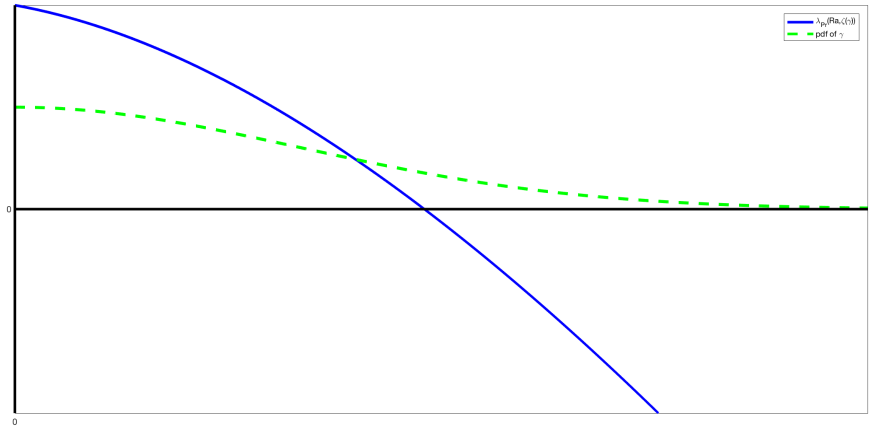
For fixed , Figure 1 depicts in the solid (blue) plot. The dashed line depicts the probability distribution of given in (27) projected to the one-dimensional subspace spanned by . If , that is, is one dimensional, the critical Rayleigh number is the value of such that the integral of the product of the curves in Figure 1 is equal to zero. An analogous principle holds in higher dimensions, that is, when .
Let us investigate the dependence of on the strength of the forcing . If increases, then the variance of the Gaussian distribution increases, meaning that the dashed curve in Figure 1 widens (recall (27)). Because the solid line (independent of ) is decreasing, decreases. On the other hand, decreasing will raise the solid curve in Figure 1, increasing (recall Theorem 2), and therefore to keep , we have to decrease the variance of the distribution, which means that is a decreasing function of .
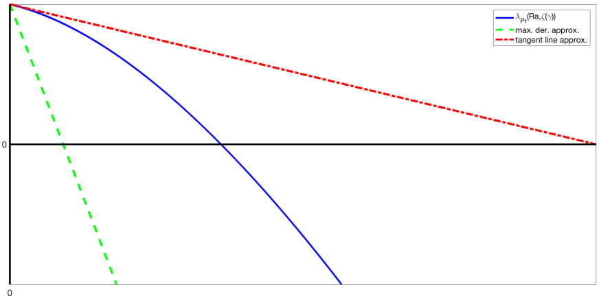
For , we combine parts 2 and 3 of Theorem 4 to obtain a decreasing tangent line approximation from above for the function , for any . Specifically, a lower bound is obtained from the linear approximation having maximal negative derivative (in any direction) given by (28). These two linear approximations illustrated in Figure 2 provide us with an upper and lower bound on the growth factor .
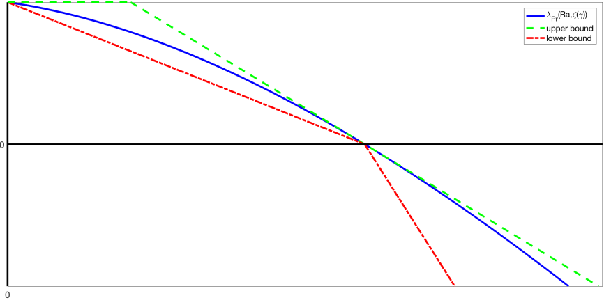
A.4.2 finally contains refined upper and lower bounds on the growth factor an their integral against the Gaussian distribution of . Figure 3 illustrates how we obtained these refined bounds. The upper bound is first obtained by applying a tangent approximation at the point (the point at which the growth factor is zero) cut off by the maximal value of the growth factor which is obtained at . Recall that this is indeed an upper bound, since is non-increasing and concave.
The lower bound is also obtained as a piece-wise linear function. First, a linear interpolation between the points at and is used for the region where the growth factor is positive. Then, a linear approximation using the maximally negative derivative originating at is used as a lower bound for negative values of . Overall, we use upper and lower bounds to estimate the dependence of the critical Rayleigh number on the stochastic forcing parameter .
First, the lower bound (depicted in Figure 3) is used to show that for small values of the internal heating the system is more stable (the critical Rayleigh number is larger with the addition of noise) than the corresponding deterministic forcing. This is stated under certain simplifying assumptions (only meant to provide an accessible proof, we do not anticipate that these restrictions are necessary) in the following theorem.
Theorem 5.
Assume that with the corresponding coefficient , , and boundary conditions (29). Denote (cf. Theorem 4)
| (32) |
Then for any there exists unique such that (recall that is a scalar and ). However, , provided . In other words the deterministic system is marginally stable at , but the stochastically forced system is almost surely stable for the corresponding internal heating.
Finally we state the final Theorem here that partially justifies the computational calculations provided below, i.e. finite sampling of the desired distribution will provide a viable approximation of the actual expected value.
Theorem 6.
Assume that in addition to the other assumptions incorporated in the previous Theorem. It follows that
| (33) | |||
| (34) |
Hence, taking the expectation of this inequality, and because are Gaussian (and hence so is ) we see that must have Gaussian tails for ( is bounded from above).
The presence of Gaussian tails justifies the computational evidence discussed below (Monte Carlo simulations of phenomena with Gaussian tails are well justified as the low probability events can safely be neglected computationally).
4 Algorithmic description, numerical comparisons, and rigorous convergence
The computation of the marginally stable parameters, i.e. those parameters for which is performed as follows. This is a root-finding problem where the Prandtl number is fixed and the stochastic heating and total number of forced modes are fixed parameters. The Rayleigh number is the independent variable. We approximate from a sample mean, and seek so that , where
| (35) |
and each is drawn independently from the stationary distribution of the conductive state. The number of samples is a parameter that we select. As is the desired situation, we will take as large as practical computational considerations will allow. Due to numerical considerations, we also must seek such that , where is also selected via numerical considerations.
For each realization of the stationary distribution, we consider the Euler-Lagrange equations for the minimization of and identify as the solution of a one-dimensional eigenvalue problem which is solved numerically via the Dedalus software package [21]. Starting with the Euler-Lagrange equations (15)–(17) for , we twice take the curl of (15) and using the fact that we have
| (36) | ||||
| (37) |
where is the third (vertical) component of the velocity and is the horizontal Laplacian. Next, we decompose and into horizontal Fourier series
where , to obtain:
| (38) | ||||
| (39) |
Since our operators are self-adjoint, and all coefficients and are real. The system also satisfies for each the boundary conditions:
| (40) |
for no-slip boundaries, where we used the identity on , which implies and by the incompressibility condition, on . Similarly, if satisfies the stress-free boundary condtions, then , and on , and consequently . Differentiating the divergence free condition with respect to , implies on , and consequently
| (41) |
for stress-free boundaries.
The numerical implementation uses a modification of the bisection root finding method on to identify the approximate , for each specified value of and the pair by taking previously computed values for nearby parameter values as an initial guess. This leads to several parameters in the algorithm that must be selected (numerical comparisons are displayed in Figure 4) for a variety of different parameters.
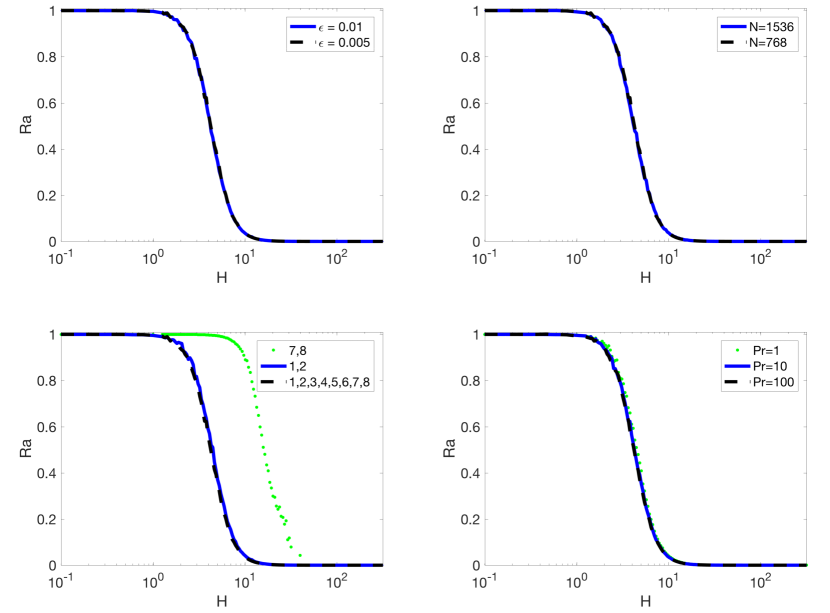
Numerical details
-
1.
Absolute error. Using as the absolute tolerance allows for a determination of at that is accurate up to 8 significant digits. We select for the results reported here. The upper left plot in Figure 4 shows the difference between the calculated critical Rayleigh number between and with the other parameters set to their default values as described below. The maximal difference between the critical Rayleigh number for is less than , jumping to a maximum of for the higher less physical values of . All other calculations reported here are for .
-
2.
Sample size. We choose Monte Carlo generated samples to compute . As a control, similar calculations were performed for , but as shown in the upper right plot of Figure 4 the differences are minimal particularly for . The maximal difference in this comparison is less than . All other parameters are the default values as explained in this section.
-
3.
Forced modes. We choose to force the first 8 modes as the default setup. The lower left plot in Figure 4 demonstrates the effects of varying the modes that are forced with all other parameters set as default values. The differences here are far more significant, with the primary conclusion being that the choice of the lowest forced mode is the most influential on the stability calculation. When only the and vertical modes are forced at sufficiently large values of , the viscous effects are not able to control the asymptotically strong, small scale oscillations causing the Monte Carlo sampling to fail to converge. This explains the jagged nature of the plot in this figure for . In addition, the root finding algorithm was unable to converge for and for larger than that shown in this plot. We expect that increasing the sample size by an order of magnitude would eliminate this issue, but would also be far to computationally prohibitive to be useful.
-
4.
Choice of the Prandtl number. The lower right plot in Figure 4 shows differences for variations on for the default parameters. There is certainly some dependence on in this case, particularly when comparing and , but these changes do not qualitatively alter the primary conclusions, and hence we choose as the default value.
-
5.
Level of discretization. We chose to discretize the eigenvalue problem with vertical Chebyshev modes. Results are identical up to 6 significant digits for as long as the highest forced mode was less than 8, i.e. . If the highest forced mode was chosen higher than then the vertical discretization would need to be increased accordingly.
-
6.
Boundary conditions. As the no-slip boundary condition is the most physically relevant to modern experiments, we focus on this boundary condition, but we have also performed comparisons with the stress-free boundary condition and found very little dependence on the velocity boundary condition. Although the actual values of are significantly different for the different boundary conditions, and within the tolerance we have admitted, the exact same transition.
In summary, the default parameters for the simulations are: , and the first 8 modes of the bulk are forced with no-slip boundaries.
5 Results
The primary takeaway from the numerical results is that weak stochastic forcing has a stabilizing effect, essentially retaining the same critical Rayleigh number for small to moderate values of as when . There is then a rapid transition (dependent on the number of modes forced for the bulk heat source) as is increased whereon the system is strongly destabilized as .
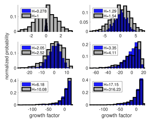
To fully investigate the transition from the conductive to the convective regime, we consider the distribution of the growth factors from the 768 samples for each value of at the transitional value of as demonstrated in Figure 5. We have chosen these particular values of as they represent different qualitative settings for the onset of instability. The variance of is clearly and unsurprisingly an increasing function of , but numerically it appears that the maximal value of is bounded from above (for rigorous proof in a special case see Lemma 22), causing the distribution of to skew strongly to the left as increases. By definition, the mean of these histograms must remain zero for all values of so that as the distribution skews negatively then must decrease toward zero rather suddenly in .
A more detailed picture regarding the appearance of these instabilities comes from considering Figure 6. Figure 6 shows the dependence of the growth factor on the critical horizontal wavenumber which indicates the spatial scale at which the instability will arise. For smaller values of the results are physically intuitive. The more unstable modes (negative values of ) arise at the larger wave-numbers, i.e. smaller scales. This indicates that when the noise is weak, there is a small-scale instability which naturally may arise as a result of the inherent randomness of the stochastic forcing. As the stochastic forcing increases in strength, this relationship breaks down to some degree insomuch that for the unstable modes occur for with the most unstable modes typically being at higher wave-numbers.
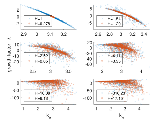
The upper bound on is also clearly seen in Fig. 6 for , and interestingly it appears that there is also an upper bound on so that even for the extreme case of , the maximal either stable or unstable is less than . These bounds on both and in the presence of a stochastic forcing with increasing variance (with respect to ) leads to an increasingly varied scattering of both and below the upper bounds, i.e. an extremely non-symmetric distribution. Even so, the largest scales indicated by remain stable.
Another interesting feature that emerges from Fig. 6 is the nearly linear relationship between and for smaller values of . Although there is significant variation from this behavior for , the same banded structure still appears in each of the plots shown in Fig. 6. This feature is indicative of the instability that arises in the deterministic setting when (near the known critical value of ), with the stochastic noise yielding stability for larger scales and instability for smaller ones. As increases this behavior still holds, but an additional trend appears wherein stable modes appear for nearly all wave-numbers below the cut-off of , and as the variance of the noise increases dramatically, the scatter about these two trends increases as well.
6 Conclusions and stability of generic stochastically driven hydrodynamic systems
We have investigated the nonlinear stability of a convective system with additive stochastic white noise on the first 8 vertical modes of the system. When the stochastic heating is weak, it has a stabilizing effect, then transitions to strongly destabilizing as the strength of the noise increases. This is an effect of the distribution of the growth factor and its dependence on the strength of the stochastic heating.
The results discussed above have demonstrated the need to better quantify the role that stochasticity plays in physically relevant fluid systems. If the internal heat source were modeled as a deterministic bulk forcing, then the stability of the resultant conductive state would be very different, particularly for the physically relevant setting of . This implies that at least in this idealized convective setting, if there is an inherently noisy source, we will miss some of the fundamental physics by modeling the system in a purely deterministic fashion. We are not claiming here that the precise nature of the noise we have chosen is the ‘best’ way to model noisy convection, but we do insist that accounting for noise in such physical systems is necessary to achieve physically realistic results.
Further considerations of the onset of convection in such stochastic settings are natural extensions of the current work. For instance, is there an analogue of the finite amplitude equations in this context, and if so, is their derivation and application the same or similar? Do coherent structures such as the roll-states present in low Rayleigh number deterministic convection exist in the stochastic setting, and if so are they defined only in a mean sense? If such structures exist, can similar statements be made regarding their stability, or does the stochastic nature of the problem preclude the utility of such investigations? Further analysis and computation is required to answer these questions, and ascertain the influence that noise can play in fully developed turbulent convection.
Finally, we note that the methodology developed in this article applies not only to Rayleigh-Bénard convection under these constraints, but is applicable to any hydrodynamic system driven by a stochastic forcing where a basic (time dependent) state still exists. In particular, we can extend this approach to shear flow, particularly where there is noise present in the induced shear boundary condition, or Rayleigh-Bénard convection when there is noise introduced through the temperature boundary condition.
Appendix A Proofs of Rigorous Bounds on the Growth Factor
A.1 A priori estimates and necessary prerequisites
We begin with an estimate that proves existence of a solution to the minimization problem and indicates that there are indeed cases such that .
Lemma 7.
Proof.
We note that for (see (23)), there is a constant such that
implying that is bounded from below. We note that contains a part which is equivalent to the norm of and and a part which is compact, and therefore is weakly lower semicontinuous in for any fixed . In addition, is weakly closed (the embedding of into is compact) in the topology of . Then from the direct methods in the calculus of variations, there exists a minimizer of (14).
Fix any compact set and let be a smooth function compactly supported in so that on . The set is a finite dimensional space of trigonometric polynomials restricted to , then all norms on are equivalent. In particular,
for any . Choose and as test functions in (14). Then is compactly supported in , is divergence free, and therefore admissible. In particular, (14) and the equivalence of norms show that
where the constants and depend only on and . The second assertion in the statement of the lemma follows immediately if is sufficiently large. ∎
Remark 8.
Uniqueness of the specified minimizer is not guaranteed, and in fact is not true in general. We can show that there is at most a one-parameter family of minimizers for each . As this does not reflect on the results that follow the details are omitted here.
In all of the following we will also need the following lemma which asserts the smoothness of the map .
Lemma 9.
For every fixed and , the map as defined in (14) is globally Lipschitz.
Proof.
We frequently make use of the following result which indicates properties obeyed by the minimizer of (14).
Lemma 10.
Proof.
As is a minimizer of , then
| (45) |
or equivalently
| (46) |
If , then by the Poincaré inequality there exists depending only on such that
| (47) | ||||
as desired. ∎
A.2 The existence of a critical Rayleigh number
The goal of the present subsection is to prove the following proposition:
Proposition 11.
The zero solution of (11)-(12) is exponentially asymptotically stable almost surely if
| (48) |
Furthermore, there is such that for any we have
| (49) |
and therefore is strictly decreasing. Also, for any , we obtain
| (50) |
and in particular is continuous.
Thus there exists at most one such that for and for .
First, however, for each we need to establish the monotonicity and continuity of and hence the existence of a critical for any fixed .
Lemma 12.
Proof.
Fix any and . Let be the minimizer of (14) as in Lemma 7. Then using Lemma 10, ,
and the monotonicity follows. If in addition , then , by Lemma 7, and consequently, by (47) we have
| (53) |
where depends only on . To prove the continuity, let be the minimizer of . Then, as above with replaced by we have the following by the Cauchy inequality
| (54) |
and the lemma follows. ∎
We note here that not only is the monotonicity with of fundamental importance in establishing a rigorous stability result, but it is also invaluable in the algorithmic development. In simulations we desire to find values of for which , and the monotonicity of allows us to know whether we need to increase or decrease . The stochastic setting is more complicated, but the same general principle applies.
Lemma 12 immediately yields the following Corollary which we phrase as a remark as it applies only to the deterministic setting:
Remark 13.
Given , there exists such that
| (55) |
holds true for all and does not hold if . When is replaced by the OU process , then in general can depend on the realization of the noise. However, due to ergodicity, we show in the proof of Proposition 11 that is almost surely constant.
Proof of Proposition 11.
Exponential decay follows once we establish that
| (56) |
Let be the unique invariant measure for the Ornstein-Uhlenbeck (OU) process defined in (8). It is known that is ergodic and supported on the whole state space . Also, by Lemma 9, the function is globally Lipschitz. In addition, since is Gaussian it necessarily has -moments for any and we have by standard ergodicity arguments [30, 31, 32] that
| (57) |
where has law on .
A.3 Concavity of the the growth factor and implications
To determine the functional dependence of on , we first investigate how depends on the source of the noise in the bulk heating. Then, we can estimate by integrating against the law of (the law of ) which has a Gaussian distribution. The primary result is Lemma 17 which establishes the concavity of . Recall the definition of from (26):
| (61) |
so that . Before establishing the concavity of we show the following deterministic uniform bound on the minimizers of (14).
Lemma 14.
Let be a minimizer of
| (62) |
If is any bounded set in then
| (63) |
Proof.
Assume that , where is the ball of radius centered at the origin. Since , then we see that
where depends on , and but is independent of and . On the other hand, for any fixed ,
Since and are fixed independently of , the desired result follows. ∎
Next, we establish the continuity of the map . Although later, we prove a stronger statement (concavity), we need the continuity as a preliminary step.
Lemma 15.
The function is continuous.
Proof.
Fix and a sequence converging to . Then by Lemma 14, the sequence of corresponding minimizers is bounded in , and therefore it has a weakly convergent subsequence converging to . By standard imbedding theorems this convergence is strong in and in particular we have and
| (64) |
Then by the weak lower semi-continuity of norms we obtain
| (65) |
Since each sequence has a convergent subsequence satisfying (65) we obtain
| (66) |
On the other hand, let be the minimizer of . Then, for any ,
| (67) | ||||
| (68) | ||||
| (69) |
and consequently
| (70) |
The continuity established in Lemma 15 allows us to prove the strong convergence of minimizers, which is an importatnt step in the proof of concavity. Specifically, fix a sequence , such that . Let be minimizers of . By Lemma 14, the sequence is bounded in , and therefore up to a sub-sequence is weakly convergent to in . The strong convergence is proved in the following corollary.
Corollary 16.
Fix a sequence , such that . Let be the minimizers of and assume is weakly convergent to in . Then is a minimizer of and converges strongly in to .
Proof.
From the continuity of and the strong convergence of cross terms (cf. (64)) we obtain
| (71) |
In addition, the weak lower semicontinuity of norms yields
| (72) |
and by (71) neither of the inequalities in (72) is strict. Hence,
| (73) |
However, weak convergence and convergence of norms in Hilbert spaces imply strong convergence, for example by the use of a parallelogram equality. This completes the proof of the desired assertion. ∎
Next, we establish the concavity of and calculate its one-sided derivatives.
Lemma 17.
The function is concave and has one sided directional derivatives. Specifically, for any one has
| (74) | ||||
| (75) | ||||
| (76) | ||||
| (77) |
where is the set of all global minimizers of .
Proof.
Fix any sequence and any . Since is the minimum over and , then
| (78) | ||||
| (79) |
Since was arbitrary, by setting for some , we obtain by linearity of that
| (80) | ||||
On the other hand, for any minimizer of we have
and consequently by linearity of
| (81) |
To prove (75), if , then by (80) and (81)
Since by Corolloary 16 the sequence converges strongly in to some we obtain
Since the sequence was arbitrary,
| (82) |
The following bound on the one-sided derivatives is used when we integrate against a Gaussian random variable below.
Corollary 18.
For any ,
| (85) |
A.4 Shape of the growth factor and consequences
In this section we establish estimates on the growth factor and obtain bounds on the critical Rayleigh number as a function of the strength of the forcing .
A.4.1 Basic estimates on the growth factor
Recall that in Lemma 17 we established that is concave, and we derived bounds on its one-sided derivatives. Next, we need to understand the behavior at .
If , then
| (88) |
Using standard arguments from the Calculus of Variations [33], we obtain that and satisfy (38) and (39) with and recall that satisfies stress-free boundary conditions (29). As in [3] we can expand into Fourier series
| (89) |
where and
| (90) |
We remark that for the no-slip boundary conditions, we have to use expansions with less explicit eigenfunctions that lead to rather complicated expressions. Thus, to avoid unnecessary and tedious manipulations, we opted to only discuss stres-free boundary conditions. Then, (38) and (39) with becomes
| (91) | ||||
| (92) |
Moreover, for given and , (91), (92) has a non-trivial solution if and only if (zero determinant and quadratic equation):
| (93) |
where we have chosen the negative sign in the quadratic root in (93) as we are interested in the smallest eigenvalue (see the discussion below (15)–(17)). To find the minimum with respect to and we first compute for each fixed and we have
Thus minimum occurs for the minimal vertical wave number . The minimum of is slightly more complicated and is analyzed in Lemma 19 below. Note that depends only on rather than on .
Recall that for each and
| (94) |
Next, we show in Lemma 21 below that if for some , then for all and hence by (19) the conductive state is trivially unstable. The following lemma gives the optimal upper bound on the Rayleigh number which guarantees that .
Lemma 19.
To simplify calculations, assume that , and define
| (95) | ||||
| (96) |
Also denote and and observe that for large , one has , and for . Then, if and only if
| (97) |
where we set if .
Proof.
From (93) and the fact that the minimum is attained at , is equivalent to
| (98) |
for all , and therefore
| (99) |
for all . The right hand side of (99) is a convex function of and its minimum is attained for . After substitution we obtain that the unique minimum (even unique critical point) is attained at . By the definition of , we have that is a vector with integer coefficients, and therefore the minimum is attained either at or . A substitution into (99) gives the desired result. ∎
Remark 20.
We want to emphasize that the restriction is not necessary for validity of Lemma 19, but reduces algebraic manipulations in the proof and very similar results hold for all .
Also, in almost all of the derivations below we will assume that to simplify the definition of and in Lemma 19, which become and . This isn’t an essential hypothesis, but it will let us avoid number theoretical discussion and make the relevant calculations more tractable.
The following result gives dependent estimates on the growth factor at and near . In other words, we estimate the behavior of the growth factor when the internal heating is very small.
Lemma 21.
Assume that , and (or equivalently , see Lemma 19). Then we have the following results dependent on the value of :
-
1.
If , then
(100) -
2.
If , then:
(101) (102) We remark that if , then .
-
3.
Finally, if , then for all .
Proof.
First we prove part 3 assuming that part 2 holds. Indeed, by part 2 for , then and , and therefore by concavity for each . Moreover, by Lemma 12 the function is non-increasing, and thus for each , as desired.
To prove parts 1 and 2, we assume note that the minimum with respect to is attained at and depends only on . To find the minimum of the function we calculate
and observe that if , then the derivative is negative, and therefore is not the minimizer. Using , we see that
whenever . Thus, is an increasing function of for . Since for some and , then the function increases if .
Thus the minimum of is attained either at or , that is, at or .
This leads to two possible cases if (99) is satisfied:
After standard algebraic manipulation we find that if and only if
| (103) |
With this in mind we are ready to analyze parts 1 and 2 of the lemma.
- 1.
-
2.
If , then and for which
(104) and the the minimum in the defintion of is achieved for
where the velocity field is . We remark that there are other minimizers shifted by a phase in -direction or with and -directions exchanged, but they give the same results. The normalization constants are chosen such that the normalization is satisfied and the velocity field is indeed incompressible. Then, by Lemma 17 we calculate the derivative
where is the coefficient for in (61). If , then is orthogonal to the test functions in so the derivative vanishes.
∎
A.4.2 Asymptotic behavior of
In all of the following we will make the simplifying assumption that , that is, only the nd mode is forced. This restriction is not necessary, but significantly reduces the calculations that follow. We do want to emphasize that forcing the nd mode does seem necessary for the results that follow, but we can not determine if this is only a product of our method of proof, or if this is in fact a physical property of the system.
Proof for Theorem 5.
Fix any . Then from Lemma 21 it follows that and , and consequently by concavity and continuity proved in Lemma 17 we have that is strictly decreasing. In particular, there is exactly one value so that .
The concavity of the growth factor yields the following bounds (see Figure 2) for each :
| (105) | ||||
| (106) | ||||
| (107) |
Because , then
| (108) |
that is, given , we obtained bounds on the strength of the deterministic internal heating that yields marginal criticality.
The concavity and (105) also yields the lower bound (see Figure 3)
| (109) | ||||
Using the hypotheses that , , and we see from Lemma 21 and Corollary 18 that
| (110) |
Now we estimate , where (recall that we are only considering ). Note that after the substitution, , we obtain that , andtherefore it suffices to assume . In particular, we bound , where .
A.4.3 Gaussian tails for the growth factor
To prove Theorem 6 we need to rigorously establish the upper and lower bound. We first investigate the upper bound. As stated in Theorem 6 we will assume that to simplify the calculations below. We also assume that the forced modes are all even although this restriction could be removed with some additional calculations. Moreover, we suppose that the horizontal domain length is an even integer. The basic approach to establish the upper bound on is to construct an admissible test function and to prove the lower bound we use general estimates.
Lemma 22.
For evenly forced modes , and horizontal domain size an even integer, we find that
| (112) |
Proof.
For (specified below), let , and . Then
| (113) |
is a divergence free vector field. Then our trial flow field is given by and the trial temperature fluctuation by . To belong to the set (see (23) for the definition), must satisfy (recalling the assumption ) which becomes the following constraint on and :
Inserting these fields into the variational form of the definition of we also arrive at
Recalling the definition (61) of and the orthogonality of trigonometric functions, we find that
Fix any and since, by assumption, is even (this choice is only to simplify the algebra at this point), depending on the sign of we set or such that the non-zero terms on the right-hand side have the same sign. Note that only the terms with the fixed can be non-zero. Moreover, because the cross term is odd in we can always choose so that this term is negative, and hence
where
Since and are even integers, we select and obtain an upper bound
| (114) |
with . After rescalling (note that and are arbitrary) and respectively by and we obtain and
| (115) |
or equivalently,
| (116) |
By standard arguments, the minimum of the right hand side is attained for , and therefore
| (117) |
for any . After we take the minimum of the right-hand side in (117) with respect to , we obtain the desired upper bound. ∎
The lower bound on the growth factor is much easier to obtain, but consequently also far less likely to be realized. Using Cauchy-Schwarz and Poincaré inequalities, definition of implying we see that
and the lower bound in Theorem 6 follows, where we used that is the principal eigenvalue of the Laplace operator on the domain .
Acknowledgements
We would like to thank G. Ahlers, C. R. Doering, B. Eckhardt, S. Friedlander, K. Lu, and J. Schumacher for helpful discussions and feedback. In particular, C. R. Doering and B. Eckhardt both gave very positive and encouraging feedback on this work before their untimely passing, and this paper is partially dedicated to their memory.
This work was conceived and completed over numerous research visits. In particular we are indebted to Mathematics departments at Brigham Young University, Université Libre de Bruxelles, Tulane University, the University of Virginia as well as the Mechanical and Aerospace Engineering department at Utah State University. We would also like to thank the Banff International Research Station which supported our work through a ‘Research in Peace fellowship’ in October of 2016. JF was partially supported by the National Science Foundation under the grant DMS-1816408. NEGH was partially supported by the National Science Foundation under the grants NSF-DMS-1313272, NSF-DMS-1816551, NSF-DMS-2108790. JPW was partially supported by the Simons Foundation travel grant under 586788 and the National Science Foundation under the grant NSF-DMS-2206762.
References
References
- [1] G. Ahlers, S. Grossmann, D. Lohse, Heat transfer and large scale dynamics in turbulent Rayleigh-Bénard convection, Review of Modern Physics 81 (2009) 503–537.
- [2] F. Chillà, J. Schumacher, New perspectives in turbulent rayleigh-bénard convection, The European Physical Journal E 35 (7) (2012) 1–25.
- [3] L. Rayleigh, On convection currents in a horizontal layer of fluid, when the higher temperature is on the under side, Philosophical Magazine and Journal of Science 32 (192) (1916) 529–546.
- [4] H. Bénard, Les Tourbillons cellulaires dans une nappe liquide, Revue génórale des Sciences pures et appliquées 11 (1900) 1261–1271.
- [5] P. G. Drazin, W. H. Reid, Hydrodynamic Stability, Cambridge University Press, 2004.
- [6] D. Goluskin, Internally heated convection and Rayleigh-Bénard convection, Springer, 2015.
- [7] G. Schubert, D. L. Turcotte, P. Olson, Mantle convection in the Earth and Planets, Cambridge University Press, 2001.
- [8] R. Kippenhahn, A. Weigert, Stellar Structure and Evolution, Springer, 1994.
- [9] J. Földes, N. Glatt-Holtz, G. Richards, E. Thomann, Ergodic and mixing properties of the boussinesq equations with a degenerate random forcing, Journal of Functional Analysis 269 (8) (2015) 2427–2504.
- [10] J. Földes, N. Glatt-Holtz, G. Richards, Large prandtl number asymptotics in randomly forced turbulent convection, submitted.
- [11] J. Földes, N. Glatt-Holtz, G. Richards, J. P. Whitehead, Ergodicity in randomly forced Rayleigh-Bénard convection, Nonlinearity 29 (11) (2016) 3309–3345.
- [12] R. Graham, H. Pleiner, Mode- mode coupling theory of the heat convection threshold, The Physics of Fluids 18 (2) (1975) 130–140.
- [13] J. Swift, P. C. Hohenberg, Hydrodynamic fluctuations at the convective instability, Physical Review A 15 (1) (1977) 319–328.
- [14] G. Ahlers, M. C. Cross, P. C. Hohenberg, S. Safran, The amplitude equation near the convective threshold: application to time-dependent heating experiments, Journal of Fluid Mechanics 110 (1981) 297–334.
-
[15]
J. Oh, J. M. Ortiz de Zárate, J. V. Sengers, G. Ahlers,
Dynamics of
fluctuations in a fluid below the onset of rayleigh-bénard convection,
Phys. Rev. E 69 (2004) 021106.
doi:10.1103/PhysRevE.69.021106.
URL https://link.aps.org/doi/10.1103/PhysRevE.69.021106 - [16] P. C. Hohenberg, J. Swift, Effects of additive noise at the onset of rayleigh-bénard convection, Physical Review A 46 (8) (1992) 4773–4785.
- [17] C. W. Meyer, G. Ahlers, D. S. Cannell, Stochastic influences on pattern formation in rayleigh-bénard convection: Ramping experiments, Physical Review A 44 (4) (1991) 2514–2537.
- [18] D. Venturi, M. Choi, G. Karniadakis, Supercritical quasi-conduction states in stochastic rayleigh–bénard convection, International Journal of Heat and Mass Transfer 55 (13) (2012) 3732–3743.
- [19] M. Hairer, J. C. Mattingly, Ergodicity of the 2d navier-stokes equations with degenerate stochastic forcing, Annals of Mathematics (2006) 993–1032.
- [20] M. Hairer, J. C. Mattingly, Spectral gaps in wasserstein distances and the 2d stochastic navier-stokes equations, The Annals of Probability (2008) 2050–2091.
- [21] K. J. Burns, G. M. Vasil, J. S. Oishi, D. Lecoanet, B. P. Brown, E. Quataert, Dedalus: A Flexible Framework for Spectrally Solving Differential Equations, in preparation http://dedalus-project.org.
- [22] G. Da Prato, J. Zabczyk, Stochastic equations in infinite dimensions, Vol. 44 of Encyclopedia of Mathematics and its Applications, Cambridge University Press, 1992.
- [23] S. Kuksin, A. Shirikyan, Mathematics of Two-Dimensional Turbulence, no. 194 in Cambridge Tracts in Mathematics, Cambridge University Press, 2012.
- [24] X. Wang, Infinite Prandtl number limit of Rayleigh-Bénard convection, Communications in Pure and Applied Mathematics 57 (2004) 1265–1285.
- [25] X. Wang, A note on long time behavior of solutions to the Boussinesq system at large Prandtl number, Contemporary Mathematics 371 (2005) 315–323.
- [26] X. Wang, Asymptotic behavior of global attractors to the Boussinesq system for Rayleigh-Bénard convection at large Prandtl number, Communications in Pure and Applied Mathematics 60 (9) (2007) 1293–1318.
- [27] X. Wang, Stationary statistical properties of Rayleigh-Bénard convection at large Prandtl number, Communications in Pure and Applied Mathematics 61 (2008) 789–815.
- [28] G. Da Prato, J. Zabczyk, Ergodicity for infinite-dimensional systems, Vol. 229 of London Mathematical Society Lecture Note Series, Cambridge University Press, Cambridge, 1996.
- [29] D. Goluskin, Internally heated convection beneath a poor conductor, Journal of Fluid Mechanics 771 (2015) 36–56.
- [30] N. Sandrić, A note on the birkhoff ergodic theorem, Results in Mathematics 72 (1) (2017) 715–730.
- [31] O. Kallenberg, O. Kallenberg, Foundations of modern probability, Vol. 2, Springer, 1997.
- [32] S. P. Meyn, R. L. Tweedie, Markov chains and stochastic stability, Springer Science & Business Media, 2012.
- [33] C. R. Doering, J. D. Gibbon, Applied Analysis of the Navier-Stokes Equations., Cambridge University Press, 1995.