X-ray Scattering from Random Rough Surfaces

Abstract

This paper presents a new method to model X-ray scattering on random rough surfaces. It combines the approaches we presented in two previous papers – PZ&LVS[zhao03] & PZ[zhao15]. An actual rough surface is (incompletely) described by its Power Spectral Density (PSD). For a given PSD, model surfaces with the same roughness as the actual surface are constructed by preserving the PSD amplitudes and assigning a random phase to each spectral component. Rays representing the incident wave are reflected from the model surface and projected onto a flat plane, which is the first order approximation of the model surface, as outgoing rays and corrected for phase delays. The projected outgoing rays are then corrected for wave densities and redistributed onto an uniform grid where the model surface is constructed. The scattering is then calculated using the Fourier Transform of the resulting distribution. This method provides the exact solutions for scattering in all directions, without small angle approximation. It is generally applicable to any wave scatterings on random rough surfaces and is not limited to small scattering angles. Examples are given for the Chandra X-ray Observatory optics. This method is also useful for the future generation X-ray astronomy missions.

1 INTRODUCTION

The study of wave scattering from rough surfaces goes back at least to Rayleigh, in his 1877 classic – The Theory of Sound[rayleigh], which led to the development of the Rayleigh criterion (see Section 2) for classifying the degree of surface roughness. Since then, the problem of scattering from random rough surfaces has been investigated by many physicists and engineers, and has been the subject of many books, including the classic – The Scattering of Electromagnetic Waves From Rough Surfaces by Beckmann and Spizzichino[beckmann] and countless research papers[ogilvy]. A good solution for X-rays scattering in grazing incidence on random rough surfaces is in high demand due to the emerging fields of X-ray optics in many applications. This problem is even more difficult due to the short wavelength (comparing to the scale of the surface roughness) and the small angle between the wave propagating direction and the surface. Most approaches in the literature make the approximation that the scattering angle is much smaller than the incident grazing angle. Some of the treatments use the approximation that the surfaces are sufficiently “smooth” so that a low order expansion in the surface height errors is adequate, and consequently are limited in their applications. Most of those methods can not obtain the scattering asymmetry around the direction of specular reflection (scattering towards versus away from the surface). These approximations are not adequate for many of the applications involving X-ray mirrors.

In 2002, we presented a SPIE paper – A new method to model X-ray scattering from random rough surfaces (PZ&LVS)[zhao03] which introduces a novel approach to the problem and gives the solution for scattering in the incident plane. In 2015, we presented a second SPIE paper – Transverse X-ray scattering on random rough surfaces (PZ)[zhao15] which gives the solution of scattering in the direction perpendicular to the incident plane. Based on the above two SPIE papers, this paper provides a complete and exact solution for X-ray scattering from random rough surfaces in all directions. This new method is generally applicable and provides the exact solution to all wave scattering problems on random rough surfaces.

In previous methods, scattered wave was usually treated separately as coherently reflected wave in the specular direction and incoherently scattered (or diffused) wave in other directions (see e.g. Simonsen[simonsen]). However, for any given wave, there is no clear distinction between “smooth” and “rough” surfaces (see Section 2), therefore it is impossible to separate scattered wave into coherently reflected and incoherently scattered waves.

The novelty of our new method is that it treats the reflected wave and scattered wave together (e.g. every ray is treated as scattered, even in the specular direction) as coherent scattering, and consequently both depend upon the surface roughness. It does not require any assumptions in order to separate the wave into reflected and scattered waves, and does not require the small angle approximation so that all the scattered rays can be traced accurately.

This new study of the century old problem is motivated by our direct involvement of the evaluation of the X-ray mirror performance aboard the Chandra X-ray Observatory (CXO) – the NASA’s third great space observatories, which has been successfully operated since July 23, 1999. It is the first, and so far the only, X-ray telescope achieving sub-arcsec angular resolution ($<0.5^{\prime\prime}$ FWHM), which let us see the X-ray Universe we had never seen before. Chandra’s spectacular success owes to the genius design and superb manufacture of its X-ray mirrors. These mirrors are the largest and the most precise grazing incidence optics ever built. At 0.84-m long and 0.6 – 1.2-m in diameters, the surface area of each mirror ranging from 1.6 to 3.2 square meters. They were polished to the highest quality ever achieved for any X-ray mirrors of this size. The surface roughness of these mirrors is comparable to or less than the X-ray wavelengths in the 0.1–10 keV band over most of the mirror surfaces. However, the mirrors are still not perfect, and consequently there are still small amount of scattered X-rays. We need an accurate model of the X-ray scattering to fully evaluate the Point Spread Function (PSF) of the CXO in order to correctly understand the scientific data. In this paper, we use the Chandra mirror surface roughness data as examples to illustrate the application of this new scattering method. This method is also useful for the future generation X-ray observatories.

2 RANDOM ROUGH SURFACES

A rough surface is a surface that deviates from the designed or assumed perfect surface upon which an incident wave achieves perfect specular reflection without energy loss to any other directions. In reality, there is no absolutely perfect surface exist. Almost all the surfaces, from the rough ocean to mountainous land, from the deck of an aircraft carrier to the finest polished mirrors, either natural or man made surfaces, are rough surfaces.

Also, no two rough surfaces are identical even they were both formed in the same well-controlled process. Not only that, every part of the same surface is also unique. We can not predict the exact roughness on one part of the surface from our knowledge of the other parts of the same surface. Its profile is simply “random”. These kind of surfaces are called random rough surfaces. Statistical methods are required to describe and study them, such as the Power Spectral Density (PSD, see Section 3). Given the PSD of a particular surface, we still can not describe the exact roughness of that surface, but we can describe a series of surfaces with the same roughness, which reflect and scatter incident waves the same way as the original surface.

When study wave reflection and scattering, a surface is called “smooth” if it specularly reflects the energy of an incident plane wave into one direction; whereas a surface is called “rough” if it scatters the energy into various directions. Based on this definition, the same surface can be called smooth or rough depends on the wavelength and incident angle. Rayleigh first studied the sound wave scattering from rough surfaces in 1877 that led to the development of the Rayleigh criterion[rayleigh]. Consider two parallel adjacent rays, with wavelength $\lambda$, incident on a rough surface with surface height difference $\sigma$, at a grazing angle $\alpha$. Upon reflection in the specular direction, the path difference between the two rays is

$$\Delta L=2\sigma sin\alpha$$ (1)

therefore the phase difference is

$$\Delta\varphi=\frac{2\pi}{\lambda}\Delta L=\frac{4\pi\sigma}{\lambda}sin\alpha$$ (2)

When the surface is perfectly “smooth”, $\sigma=0$ hence $\Delta\varphi=0$; two rays are in phase, therefore reflect specularly. When $\Delta\varphi=\pi$, two rays cancel each other, there is no specular reflection; hence the surface is called “rough”. In this case, the energy are scattered into other directions due to the energy conservation. By arbitrarily choosing the value halfway between these two extreme cases, $\Delta\varphi=\pi/2$, we obtain the Rayleigh criterion for smooth surface:

$$\frac{4\pi\sigma}{\lambda}sin\alpha<\frac{\pi}{2}~{}~{}~{}~{}~{}\Longrightarrow~{}~{}~{}~{}~{}\sigma<\frac{\lambda}{8~{}sin\alpha}$$ (3)

In reality, there is no clear cut between the so-called “smooth” and “rough”. A surface satisfying the Rayleigh criterion can only be considered as “nearly” smooth. Unless $\sigma=0$, there is always a small amount of energy being scattered into non-specular directions. As we shall see, the Chandra telescope mirrors do satisfy the Rayleigh criterion. But just that small amount of energy scattered away from the specular direction needs to be taken into account in order to fully understand its PSF. In this sense, all the surfaces can be considered as “rough”, because there is no real surfaces are perfect ($\sigma=0$). Table 1 gives some examples of “smooth” surface based on the Rayleigh criterion.

Table 1: Examples of “smooth” surface based on the Rayleigh criterion

Surface	Wave frequency/energy	$\lambda$	$\alpha$	$\sigma$
Airport radar dish	$\sim$3 GHz	$\sim$10 cm	$\sim$80∘	$<$ 1.3 cm
Satellite TV dish	$\sim$10 GHz	$\sim$30 mm	$\sim$60∘	$<$ 4.3 mm
Mirror in your bath room	$\sim$545 THz	$\sim$550 nm	90∘	$<$ 69 nm
Chandra X-ray Observatory	0.1 – 10 keV	1.24Å – 124Å	27.1′ – 51.3′	$<$ 10Å

3 Power Spectral Density of Rough Surfaces

A rough surface is described, statistically, by its surface Power Spectral Density (PSD) as a function of the surface spatial frequency $f$. Consider a 1-dimensional surface with length $L$ and surface height (i.e. deviation from a perfectly flat surface): $z=h(x)$. Its PSD is defined as:

$$PSD(f)\equiv 2W_{1}(f)=\frac{2}{L}~{}\left|\int_{-L/2}^{L/2}e^{\imath 2\pi xf}h(x)dx\right|^{2}$$ (4)

The PSD, as it is defined, is the “spectrum” of the surface roughness. Its value at $f$ is simply the “power” at that frequency. It is easy to distinguish between periodic and random rough surfaces from their PSDs. For periodic rough surfaces, there are some “spectral lines” in their PSDs; whereas there are no lines exist for a real random rough surface.

Given a PSD function $2W_{1}$, the surface roughness amplitude RMS in the frequency band of $f_{1}$ – $f_{2}$ (both $f_{1}$ and $f_{2}$ are positive) can be calculated as:

$$\sigma_{f_{1}-f_{2}}^{2}=\int_{f_{1}}^{f_{2}}2W_{1}(f)df$$ (5)

For a 2-D random rough surface, the two orthogonal dimensions can be treated separately and each as a 1-D surface. So the above definitions are still valid. For example, for the grazing incident rays upon a 2-D random rough surface, one dimension can be chosen as the intersection of the incident plane and the surface. The scattered rays will remain in the incident plane. This case is called the in-plane scattering. The second dimension can be chosen as the direction on the surface but perpendicular to the incident plane. In this case the scattered rays are out of the incident plane. This case is called the out-plane, or transverse, scattering. Since the surface roughness can be different in these two directions, their PSDs can also be different.

4 Chandra X-ray optics

The Chandra X-ray optics – High Resolution Mirror Assembly (HRMA) – is an assembly of four nested Wolter Type-I (paraboloid and hyperboloid) grazing incidence mirrors made of Zerodur and coated with iridium (Ir)[lvs97, zhao97, zhao98, zhao04]. The eight mirrors are named P1,3,4,6 (paraboloid) and H1,3,4,6 (hyperboloid), due to historical reasons (there were 6 mirror pairs when the HRMA was designed and two pairs were later removed to reduce the cost). The mirror elements were polished by the then Hughes Danbury Optical Systems, Inc. (HDOS). The surface roughness was measured during the HDOS metrology measurements after the final polishing, but before the iridium coating[reid95]. Tests conducted on sample flats before and after the coating indicate that the coating does not change the surface roughness.

The instruments used for the measurements were the Circularity and Inner Diameter Station (CIDS), the Precision Metrology Station (PMS), and the Micro Phase Measuring Interferometer (MPMI, aka WYKO). The CIDS was used to determine the circularity and the inner diameters. The PMS was used to measure along individual axial meridians. With these two instruments, HDOS essentially measured the ‘hoops’ and ‘staves’ of each mirror barrel, and thus mapped the entire surface. The micro-roughness was sampled along meridian at different azimuths using the WYKO instrument at three different magnifications ($\times$1.5, $\times$10 & $\times$40)[reid95, zhao95].

These metrology data were Fourier transformed and filtered. The low frequency parts of the CIDS and PMS data were used to form mirror surface deformation (from the designed mirror surface) maps. The high frequency parts of the PMS data and the WYKO data were used to estimate the surface micro-roughness. Both of them are parts of the HRMA model we built for the raytrace simulation of the Chandra performance.

The mirror surface micro-roughness has little variation with azimuth, but tends to become worse near the mirror ends. Table 2

Table 2: HRMA Mirror Sections and Their Surface Roughness

HRMA	Sections											Num of
Mirror	Surface Roughness Amplitude RMS $\sigma_{1-1000/{\rm mm}}$ (Å)											Sections
P1		LC	LB	LA	M (88%)	SA	SB	SC				7
		50.3	8.49	4.51	3.58	4.91	5.94	53.9
P3			LB	LA	M (92%)	SA	SB					5
			5.37	5.26	1.96	2.38	4.83
P4			LB	LA	M (93%)	SA	SB					5
			6.41	3.15	2.57	3.21	6.81
P6			LB	LA	M (94%)	SA	SB					5
			37.1	5.23	3.34	5.65	20.9
H1	LD	LC	LB	LA	M (88%)	SA	SB	SC	SD	SE	SF	11
	26.9	5.34	3.64	3.34	3.32	3.32	3.32	3.32	3.53	7.30	60.3
H3		LC	LB	LA	M (92%)	SA	SB	SC	SD			8
		4.87	2.90	2.23	2.08	2.08	2.10	3.95	5.56
H4	LD	LC	LB	LA	M (93%)	SA	SB	SC	SD	SE		10
	7.18	3.83	2.61	2.57	2.36	2.36	2.74	2.68	4.01	29.4
H6	LD	LC	LB	LA	M (94%)	SA	SB	SC	SD	SE		10
	19.0	4.92	2.51	2.23	1.95	1.95	1.95	2.07	2.96	15.9
Total												61

shows the surface roughness of the 61 HRMA mirror sections based on their roughness. The number underneath each section name is the surface roughness amplitude RMS, $\sigma_{1-1000/{\rm mm}}$, calculated according to Eq. (5) for $f=1-1000~{}$mm^-1. Each mirror is 838.2 mm in length. The middle sections (M), which are the best polished and hence have the lowest PSDs, cover most part of the mirror surface (the number in parentheses after each M denote the percentage coverage). The $\sigma$’s for the M sections are only 1.9–3.6 Å. The end sections, where the $\sigma$’s are relatively higher, cover a very small part of the mirror ($<1\%$), and hence contribute very little to the mirror performance.

It is seen that all the middle sections are polished to the satisfaction of the Rayleigh criterion as “smooth” surface (Eq. 3 and Table 1), therefore they provide very good reflections in the specular direction for X-rays.

However, since the mirror surfaces are not perfect, there are still small among of scatterings from the middle sections. In addition, the end sections are not “smooth” based on the Rayleigh criterion. So we need to have a good scattering model in order to understand the PSF of the telescope.

Figures 2 and 2 show the PSDs of the M (middle) and SC (small end) sections of P1. P1 and H1 are the first polished mirror pair and are slightly “rougher” than other pairs (see Table 2). The (colored) dash and dotted lines show the data from different measurements: the PMS data are in the low frequency range ($f=0.001-0.3$ mm^-1); the WYKO data with 3 magnifications are in the higher frequency range ($f=0.3-1000$ mm${}^{-1})$. The black solid lines are the combined PSDs from all the measurements. The SC section obviously is much rougher than the M section.

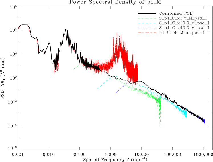
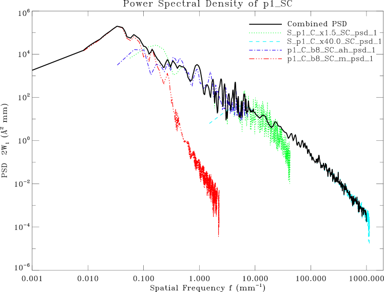
Figure 1: Surface PSD of Chandra mirror P1-M, the middle section of mirror P1.

Figure 2: Surface PSD of Chandra mirror P1-SC, the small end section of mirror P1.

5 MODEL SURFACES

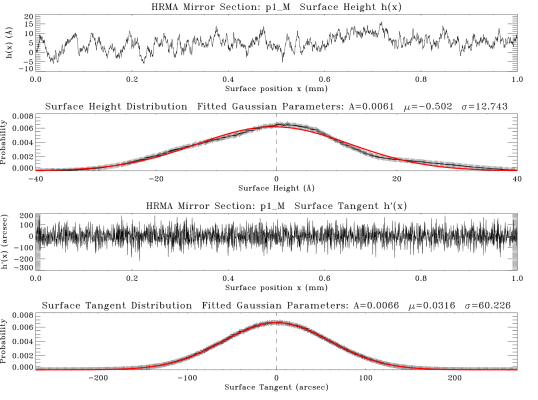
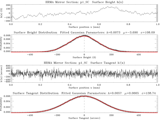
Figure 3: A model surface of mirror section P1-M, which covers 88% of the P1. The top panel shows the surface height deviation, $h(x)$, for a 1 mm section of the model surface; the second panel shows the deviation distribution of the entire surface; the third panel shows the surface tangent, $h^{\prime}(x)$, for the same section. The bottom panel shows the surface tangent distribution of the entire surface. Both distribution curves match closely with an ideal Gaussian (solid red curve).

Figure 4: A model surface mirror section P1-SC, which is the ‘worst” end-section of the P1 mirror.

A random rough surface can be described by its PSD. Most of the existing methods calculate the scattering from the surface PSD. However, our method calculates the scattering directly from the surface profile. Therefore, we first need to construct a model surface that is based on its PSD. From a random rough surface profile, we can derive a unique PSD. But from this unique PSD, we can not reconstruct the original surface, because the phase information was lost when deriving the PSD. However, we can construct any number of model surfaces with the same roughness as the original one from its PSD by assigning different random phase factors to the spectral components.

As mentioned in Section 3, for a 2-D surface, we can treat the two orthogonal dimensions separately and each as a 1-D surface. To construct a 1-D model surface with length $L$, we need to derive $N$ consecutive surface heights, $h_{i}=h(x_{i})$, with a fixed interval $\Delta x$ to cover the surface (i.e. $N\Delta x=L$, where $\Delta x$ is the spatial resolution of the model surface), and their surface tangents, $h^{\prime}_{i}=h^{\prime}(x_{i})$. Appendix A shows that $h_{i}$ and $h^{\prime}_{i}$ can be computed from the surface PSD using the following Fourier transforms:

$$h_{i} = \frac{1}{N}\sum^{N/2}_{j=-(N/2-1)}~{}H_{j}~{}e^{-\imath\frac{2\pi ij}{N}}$$ (6)

$$h^{\prime}_{i} = \frac{1}{N}\sum^{N/2}_{j=-(N/2-1)}~{}\left(-\imath 2\pi f_{j}~{}H_{j}\right)~{}e^{-\imath\frac{2\pi ij}{N}}$$ (7)

where $f_{j}$ is the surface spatial frequency; $H_{j}=N\sqrt{\frac{PSD(f_{j})~{}\Delta f}{2}}~{}e^{\imath\varphi_{j}}$, $\Delta f=1/N\Delta x$, $\varphi_{j}$ is the assigned random phase factor. Since both $h_{i}$ and $h^{\prime}_{i}$ are real, this requires $H_{-j}=H_{j}^{*}$, i.e. $PSD(f_{-j})=PSD(f_{j})$ and $\varphi_{-j}=-\varphi_{j}$.

To construct the model surfaces of HRMA, we choose $N=2^{21}$ and $\Delta x=0.0004$ mm. So $L=N\Delta x=838.86$ mm, and $\Delta f=1/N\Delta x=0.001192$ mm^-1. Figures 4 and 4 show one set of model surface sections P1-M and P1-SC, constructed using their PSDs (Fig. 2 and 2) with Eqs. (6) and (7).

Each HRMA mirror is a 2-D surface. For any given point on the surface, its two orthogonal dimensions are the one along the meridian and the one along the azimuth. The roughness along the meridian causes the in-plane scattering. The roughness along the azimuth causes the out-plane scattering. Depending on the polishing method, the roughness can be different in these two directions. For the HRMA, however, the metrology data did not show this difference. Therefore we treat these two dimensions as having the same roughness, i.e. the same PSD is used to construct the model surface profiles in both directions.

6 In-plane scattering from model surfaces

In this section, we derive the in-plane scattering formulae of plane incident waves from a model random rough surface. Details of the derivations can be found in Appendices B and C.

We assume the surfaces are sufficiently smooth so that: 1) there is no shadowing of one part of the surface by another; and 2) there is no reflection from one part of the surface to another, i.e. there are no multiple reflections by the same surface. For an incident plane wave with grazing angle $\alpha$, the first condition requires that the absolute values of all the surface tangents, $|h^{\prime}_{i}|$, are less than $\alpha$. The second condition requires $|h^{\prime}_{i}|$ less than $\alpha/2$ (when $h^{\prime}_{i}=-\alpha/2$, the reflected wave is parallel to the surface). The first condition is automatically satisfied when the second condition is met. So the surface roughness condition for applying this method is:

$$|h^{\prime}_{i}|<\frac{\alpha}{2}$$ (8)

This condition is easily satisfied for all 61 HRMA sections, as can be seen by comparing the tangent distributions in Figures 4 and 4 with the mean grazing angles of the four HRMA mirror pairs ($51.26^{\prime},41.27^{\prime},36.43^{\prime},27.08^{\prime}$).

The scattering formula is given by Eq. (74) in Appendix C.4 as the discrete Fourier transform of the field ${\bf E}_{i}$, on ${\bf x}$-axis, in flat surface $S_{0}$:

$$I(\theta_{j+q/p}) = \mathcal{A}\,\left(\frac{\Delta x\,sin(\alpha-\theta_{j+q/p})}{\lambda}\right)^{2}~{}\left|\sum^{N/2}_{i=-(N/2-1)}~{}\left({\bf E}_{i}e^{\imath\frac{2\pi iq/p}{N}}\right)~{}e^{\imath\frac{2\pi ij}{N}}\right|^{2}\hskip 14.45377pt(q=0,1,\ldots,p-1)$$ (9)

where the scattering field intensity $I$ is a function of the scattering angle $\theta_{j+q/p}$, which is the deviation from the specular reflection direction ($\theta>0$ is towards the surface, $\theta<0$ is aways from the surface); $\lambda$ is the wavelength; ${\bf E}_{i}$ is the field amplitude, after the reflection, at uniform grid $x_{i}$ on ${\bf x}$-axis, where the model surface was constructed. ${\bf E}_{i}$ is a function of the incident wave, the model surface height and tangent, and the local reflectivity. $\mathcal{A}$ is a normalization factor given by Eq (79). Again we choose $N=2^{21}$ to cover the entire length of the model surface.

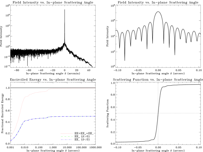
Figure 5: The in-plane scattering of 1.49 keV X-rays at 51.26^′ grazing incident angle from the model surface P1-M. The top-left panel shows the scattering field intensity $I$ versus the scattering angle $\theta$. The very sharp peak is at the specular direction $\theta=0$. The asymmetric scattering profile wrt to $\theta=0$ is clearly shown. The top-right panel is the same plot but zoomed into the core of the peak; it shows the Fraunhofer diffraction pattern due to the finite mirror length. The bottom-left panel shows the fractional Encircled Energy (EE) versus $\theta$, for both sides of the specular direction, and also their sum. The bottom-right panel shows the scattering function $\mathcal{S}$ versus $\theta$ in the same range as the top-right panel.

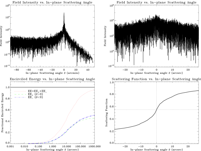
Figure 6: Out-plane scattering from model surface P1-SC, with the same description as Fig. 5. Since P1-SC is much rougher, it has much broader scattering profile than P1-M.

Figures 5 and 6 show the in-plane scattering results, using Eq (9), for 1.49 keV X-rays incident upon the mirror P1 at its mean grazing angle (51.26^′). The top two panels show the scattering intensity $I$ versus the scattering angle $\theta$. Positive $\theta$ is defined as the scattering towards the surface; negative $\theta$ is the scattering away from the surface. The sharp peak of specular reflection (top-left) and the Fraunhofer diffraction pattern (top-right) are shown as expected. The bottom two panels show the fractional Encircled Energies $EE_{+},EE_{-},EE$ and the scattering function $\mathcal{S}$, defined as:

$$EE_{+}(\theta) \equiv \frac{1}{\mathcal{E}_{s}}\int_{0}^{\theta}\,I(\theta_{j})\,d\theta_{j}~{}=~{}\frac{1}{\mathcal{R}\,\mathcal{E}_{i}}\int_{0}^{\theta}\,I(\theta_{j})\,d\theta_{j}$$ (10)

$$EE_{-}(\theta) \equiv \frac{1}{\mathcal{E}_{s}}\int_{-\theta}^{0}\,I(\theta_{j})\,d\theta_{j}~{}=~{}\frac{1}{\mathcal{R}\,\mathcal{E}_{i}}\int_{-\theta}^{0}\,I(\theta_{j})\,d\theta_{j}$$ (11)

$$EE(\theta) \equiv \frac{1}{\mathcal{E}_{s}}\int_{-\theta}^{\theta}\,I(\theta_{j})\,d\theta_{j}~{}=~{}\frac{1}{\mathcal{R}\,\mathcal{E}_{i}}\int_{-\theta}^{\theta}\,I(\theta_{j})\,d\theta_{j}$$ (12)

$$\mathcal{S}(\theta) \equiv \frac{1}{\mathcal{E}_{s}}\int_{-\pi+\alpha}^{\theta}\,I(\theta_{j})\,d\theta_{j}~{}=~{}\frac{1}{\mathcal{R}\,\mathcal{E}_{i}}\int_{-\pi+\alpha}^{\theta}\,I(\theta_{j})\,d\theta_{j}$$

where $\mathcal{E}_{i}$, $\mathcal{E}_{s}$ and $\mathcal{R}$ are the total incident and scattered energy, and the reflectivity of the rough surface as defined in Appendix C.5. The scattering function $\mathcal{S}$ is the integral of the scattering intensity $I$ over the angular space $\pi$ above x-axis. It is simply the probability function (in the domain of [0,1]) of the in-plane scattering angle $\theta$.

7 Out-plane scattering from model surfaces

When the scattering angle is small comparing to the incident grazing angle, the transverse scattering angle, i.e. the out-plane scattering, is smaller than the in-plane scattering angle by approximately a factor of the grazing angle. Therefore traditionally the transverse scattering was treated by simply multiplying the in-plane scattering by a factor of the grazing angle $\alpha$ in radians. This is a good approximation for small angle scatterings. However, since our method is not limited to small angle scatterings, the above approximation is no longer valid when the scattering angle approaches the grazing angle. In this section, we derive the exact equations for the transverse scattering. Details of the derivation can be found in Appendix D.

The out-plane scattering formula is given by the discrete Fourier transform of the field ${\bf E}_{i}$, on ${\bf y}$-axis, in flat surface $S_{0}$, as shown in Eq (105) in Appendix D.4:

$$J(\eta_{j+q/p}) = \mathcal{B}\,\left(\frac{\Delta y\,sin\,\alpha}{\lambda}\right)^{2}~{}\left|\sum^{N/2}_{i=-(N/2-1)}~{}\left({\bf E}_{i}e^{\imath\frac{2\pi iq/p}{N}}\right)~{}e^{\imath\frac{2\pi ij}{N}}\right|^{2}\hskip 21.68121pt(q=0,1,2,\ldots,p-1)$$ (14)

where the scattering intensity $J$ is a function of the transverse scattering angle $\eta_{j+q/p}$, which is the deviation from the specular reflection direction; $\lambda$ is the wavelength; ${\bf E}_{i}$ is the field amplitude, after the reflection, at uniform grid $y_{i}$ on ${\bf y}$-axis, where the model surface was constructed. ${\bf E}_{i}$ is a function of the incident wave, the model surface height and tangent, and the local reflectivity. $\mathcal{B}$ is a normalization factor given by Eq (110).

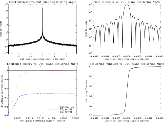
Figure 7: The out-plane scattering of 1.49 keV X-rays at 51.26^′ grazing incident angle from the model surface P1-M. The top-left panel shows the transverse scattering field intensity $J$ versus the scattering angle $\eta$. Due to the symmetric nature of the transverse scattering, the sign of $\eta$ can be defined in either direction of the ${\bf y}$-axis. The very sharp peak is at the specular direction $\eta=0$ (and $\theta=0$). The transverse scattering profile is symmetric wrt to $\eta=0$ as expected. The top-right panel is the same plot but zoomed into the core of the peak; it shows the Fraunhofer diffraction pattern due to the finite mirror length. The bottom-left panel shows the fractional Encircled Energy (EE) versus $\eta$, for both sides of the specular direction, and also their sum. The bottom-right panel shows the transverse scattering function $\mathcal{T}$ versus $\eta$ in the same range as the top-right panel. In all the panels except for the top-left, the scale of the X-axis is smaller than that in the same panel of Fig. 5 by a factor of the grazing angle (51.26^′ = 0.01491 rad).

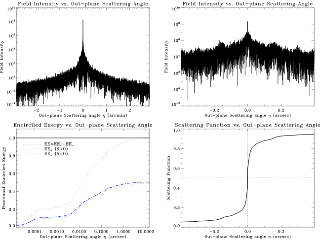
Figure 8: Out-plane scattering from model surface P1-SC, with the same description as Fig. 7. It has much broader scattering profile than P1-M.

Figures 7 and 8 show the out-plane scattering results, using Eq (14), for 1.49 keV X-rays incident upon the mirror P1 at its mean grazing angle (51.26^′). The top two panels show the transverse scattering intensity $J$ versus the scattering angle $\eta$. The sharp peak of specular reflection (top-left) and the Fraunhofer diffraction pattern (top-right) are shown as expected. The bottom two panels show the fractional Encircled Energies $EE_{+},EE_{-},EE$ and the transverse scattering function $\mathcal{T}$ defined as:

$$EE_{+}(\eta) \equiv \frac{1}{\mathcal{E}_{s}}\int_{0}^{\eta}\,J(\eta_{j})\,d\eta_{j}~{}=~{}\frac{1}{\mathcal{R}\,\mathcal{E}_{i}}\int_{0}^{\eta}\,J(\eta_{j})\,d\eta_{j}$$ (15)

$$EE_{-}(\eta) \equiv \frac{1}{\mathcal{E}_{s}}\int_{-\eta}^{0}\,J(\eta_{j})\,d\eta_{j}~{}=~{}\frac{1}{\mathcal{R}\,\mathcal{E}_{i}}\int_{-\eta}^{0}\,J(\eta_{j})\,d\eta_{j}$$ (16)

$$EE(\eta) \equiv \frac{1}{\mathcal{E}_{s}}\int_{-\eta}^{\eta}\,J(\eta_{j})\,d\eta_{j}~{}=~{}\frac{1}{\mathcal{R}\,\mathcal{E}_{i}}\int_{-\eta}^{\eta}\,J(\eta_{j})\,d\eta_{j}$$ (17)

$$\mathcal{T}(\eta) \equiv \frac{1}{\mathcal{E}_{s}}\int_{-\pi/2}^{\eta}\,J(\eta_{j})\,d\eta_{j}~{}=~{}\frac{1}{\mathcal{R}\,\mathcal{E}_{i}}\int_{-\pi/2}^{\eta}\,J(\eta_{j})\,d\eta_{j}$$

where $\mathcal{E}_{i}$, $\mathcal{E}_{s}$ and $\mathcal{R}$ are the total incident and scattered energy, and the reflectivity of the rough surface as defined in Appendix D.5. The scattering function $\mathcal{T}$ is the integral of the scattering intensity $J$ over the angular space $\pi$ above y-axis. It is simply the probability function (in the domain of [0,1]) of the out-plane scattering angle $\eta$.

Now let’s compare Fig. 7 of the out-plane scattering with Fig. 5 of the in-plane scattering, for the mirror section P1-M. The top-left panels show the scattering field intensity versus the scattering angle: the out-plane scattering is symmetric wrt to the specular direction; while the in-plane scattering is asymmetric. This difference is as expected due to the scattering geometry. The other three panels show the core of the intensity, encircled energy and scattering function versus the scattering angle, with the scale of the X-axis in Fig. 7 smaller than that of in Fig. 5 by a factor of the grazing angle (51.26^′ = 0.01491 rad). It is seen that these three panels are very similar to each other in the two figures. This indicates that, when the surface is sufficiently “smooth”, therefore the scattering angle is small, the out-plane scattering angle is approximately smaller than the in-plane scattering angle by a factor of the grazing angle, as shown in Appendix D.6.

Next let’s compare Fig. 8 with Fig. 6, for the mirror section P1-SC. The top-left panels still show the symmetric versus asymmetric profile of the out-plane and in-plane scattering. But, because the P1-SC section is much rougher and therefore scattering angle is larger, the other three panels look different, even the scale of the X-axis in Fig. 8 is still smaller than that of in Fig. 6 by a factor of 0.01491. This indicates that, when the surface is “rough” so that the scattering angles are large, the small angle approximation treatment for the out-plane scattering is no longer valid. An exact solution of of the out-plane scattering, independent of the in-plane scattering, is required for the general case.

8 General solution of scattering from random rough surfaces

With the in-plane and out-plane scattering formulae Eqs (9) and (14), and their scattering functions Eqs (6) and (7), the general solution of scattering from random rough surfaces can be obtained.

The solution can easily be applied in any raytrace or Monte Carlo simulations. For a monotonic plane wave with a fixed incident angle $\alpha$, if the surface is perfect, the plane wave is reflected in the specular direction, with the reflecting angle $\beta=\alpha$. If the surface is not perfect, then every ray is treated as a scattered ray, even in the specular direction.

First, two scattering tables are generated using the in-plane and out-plane scattering functions $\mathcal{S}(\theta)$ and $\mathcal{T}(\eta)$, for the given photon energy $\varepsilon$ and incident angle $\alpha$. Then for each ray, two independent uniform random numbers selected in the domain of [0,1] are used to find the in-plane and out-plane scattering angles $\theta$ and $\eta$ from the tabulated $\mathcal{S}(\theta)$ and $\mathcal{T}(\eta)$ (interpolation is needed in this process). Finally the reflected ray is deflected from its specular direction by $\theta$ (in-plane) and $\eta$ (out-plane), respectively. The result of this raytrace simulation yields a scattering pattern in a 2-D angular space for the given plane wave.

However, the above process is only good for one fixed energy and incident angle. For a real source with an energy spectrum and a range of incident angles (e.g. photons hit HRMA mirrors at slightly different angles on the same paraboloid or hyperboloid surface), the above process needs to be expanded to more general cases.

Each pair of scattering functions $\mathcal{S}(\theta)$ and $\mathcal{T}(\eta)$ are good only for a given photon energy $\varepsilon$ and incident angle $\alpha$. So theoretically, to cover an energy spectrum with a range of incident angles, many $\mathcal{S}$ and $\mathcal{T}$ are required on a 2-D grid of [$\varepsilon$, $\alpha$]. Obviously, this requires enormous amount of computation time and makes the calculation very slow and cumbersome. However, it can be shown that, to a very high degree of accuracy, for small variations of $\varepsilon$ and $\alpha$, $\mathcal{S}$ and $\mathcal{T}$ only depend on the product of $\varepsilon$ and $sin\alpha$, instead of depending on them separately. This fact greatly reduces the amount of computations. Instead of on 2-D, $\mathcal{S}$ and $\mathcal{T}$ only need to be generated on a 1-D grid of $\varepsilon sin\alpha$.

Define $\gamma\equiv\varepsilon sin\alpha$. Since

$$\lambda=\frac{c}{\nu}=\frac{hc}{\varepsilon}$$ (19)

where $c$ is the speed of light; $\nu$ is the photon frequency; $h$ is the Planck constant. The scattering intensity $I(\theta_{j})$ and $J(\eta_{j})$ (Eqs (9) and (14)) on the 1-D grid of $\gamma$ can be written as:

$$I_{\gamma}(\theta_{j+q/p}) = \mathcal{A}\,\left(\frac{\Delta x\,\varepsilon\,sin(\alpha-\theta_{j+q/p})}{hc}\right)^{2}~{}\left|\sum^{N/2}_{i=-(N/2-1)}~{}\left({\bf E}_{i_{in}}e^{\imath\frac{2\pi iq/p}{N}}\right)~{}e^{\imath\frac{2\pi ij}{N}}\right|^{2}\hskip 14.45377pt(q=0,1,\ldots,p-1)\hskip 14.45377pt$$ (20)

$$J_{\gamma}(\eta_{j+q/p}) = \mathcal{B}\,\left(\frac{\Delta y\,\varepsilon\,sin\,\alpha}{hc}\right)^{2}~{}\left|\sum^{N/2}_{i=-(N/2-1)}~{}\left({\bf E}_{i_{out}}e^{\imath\frac{2\pi iq/p}{N}}\right)~{}e^{\imath\frac{2\pi ij}{N}}\right|^{2}\hskip 57.81621pt(q=0,1,\ldots,p-1)\hskip 14.45377pt$$ (21)

where ${\bf E}_{i_{in}}$ and ${\bf E}_{i_{out}}$ are the field amplitudes uniformly distributed on ${\bf x}$ and ${\bf y}$-axis (with even spacing $\Delta x$ and $\Delta y$) in flat surface $S_{0}$, for in- and out-plane scatterings respectively. They are functions of local surface height, tangent, reflection coefficient, as well as the photon energy $\varepsilon$ and incident angle $\alpha$, as explicitly expressed in Eq (69) in Appendix C.3 and Eq (100) in Appendix D.3.

The scattering functions $\mathcal{S}(\theta)$ and $\mathcal{T}(\eta)$ (Eqs (6) and (7)) on the 1-D grid of $\gamma$ can be written as:

$$\mathcal{S}_{\gamma}(\theta) = \frac{1}{\mathcal{R}\,\mathcal{E}_{i}}\int_{-\pi+\alpha}^{\theta}\,I(\theta_{j})\,d\theta_{j}$$ (22)

$$= \frac{1}{\mathcal{R}_{in}\,N\varepsilon}\int_{-\pi+\alpha}^{\theta}\,I_{\gamma}(\theta_{j})\,d\theta_{j}$$

$$\mathcal{T}_{\gamma}(\eta) = \frac{1}{\mathcal{R}\,\mathcal{E}_{i}}\int_{-\pi/2}^{\eta}\,J(\eta_{j})\,d\eta_{j}$$ (23)

$$= \frac{1}{\mathcal{R}_{out}\,N\varepsilon}\int_{-\pi/2}^{\eta}\,J_{\gamma}(\eta_{j})\,d\eta_{j}$$

where $\mathcal{R}_{in}$ and $\mathcal{R}_{out}$ are the in- and out-plane reflectivities as defined by Eq (78) in Appendix C.5 and Eq (109) in Appendix D.5.

The general solution of scattering of plane wave in the photon energy range [$\varepsilon_{0},\varepsilon_{1}$], ($\varepsilon_{0}<\varepsilon_{1}$), and incident angle range [$\alpha_{0},\alpha_{1}$], ($\alpha_{0}<\alpha_{1}$), can be obtained in following steps:

1. Perform Fast Fourier Transform (FFT) to calculate the scattering intensities $I_{\gamma}(\theta_{j})$ and $J_{\gamma}(\eta_{j})$, using Eqs (20) and (21), on the 1-D grid in the domain of $\gamma\in[\varepsilon_{0}sin\alpha_{0},\varepsilon_{1}sin\alpha_{1}]$. A density of $\Delta\gamma/\gamma\approx 2\%$ is sufficient for accurate interpolations. (e.g. for $\frac{\varepsilon_{1}sin\alpha_{1}}{\varepsilon_{0}sin\alpha_{0}}-1\approx 0.2$, $\gamma$ assumes 11 values uniformly distributed in $[\varepsilon_{0}sin\alpha_{0},\varepsilon_{1}sin\alpha_{1}]$ is sufficient.

2. For each $\gamma$, calculate and tabulate the scattering functions $\mathcal{S}_{\gamma}(\theta)$ and $\mathcal{T}_{\gamma}(\eta)$, using Eqs (22) and (23). The resulting scattering tables can be read as the reverse functions of $\theta(\mathcal{S}_{\gamma})$ and $\eta(\mathcal{T}_{\gamma})$, with both $\mathcal{S}_{\gamma}$ and $\mathcal{T}_{\gamma}$ assume uniform grid of 100,000 points in the domain of [0,1] in order to achieve good angular resolutions.

3. For each incident ray with energy $\varepsilon$ and incident angle $\alpha$, use two independent uniform random numbers selected in the domain of [0,1] and interpolation to find its in-plane and out-plane scattering angles $\theta$ and $\eta$ from the scattering tables.

4. Finally, the ray is deflected from its specular direction by $\theta$ (in-plane) and $\eta$ (out-plane), respectively.

The above process yields a scattering pattern in the 2-D angular space for the plane wave with a finite range of photon energies and incident angles. This completes the general solution of wave scattering from random rough surfaces.

9 SUMMARY

The exact solution of wave scattering from random rough surfaces are derived. This solution provides a new method to solve the long standing problem of scattering from random rough surfaces in an accurate and more general way. This new method treats both the reflected wave and scattered wave together as coherent scattering, instead of treating them separately as coherent reflection and incoherent (diffuse) scattering. Table 3 compares different aspects of the scattering treatment between the traditional method and the this new method.

Table 3: Comparing Traditional Method with the New Method of scattering from Random Rough Surfaces

Aspect	Traditional Method	New Method
Scatter and reflection	treated separately as coherent	treated together as
	reflection and diffuse scattering	coherent scattering
Scattered rays	only some rays are treated as scattered	every ray is treated as scattered
Scattering angle	much smaller than the grazing angle	no restrictions
In-plane scattering	symmetric wrt specular direction	asymmetric wrt specular direction
Out-plane scattering	grazing angle times in-plane scattering	solved independently

The major advantage of this new method is that it is not limited by the small angle approximation and gives accurate solutions to in-plane and out-plane scatterings of any angular size. This made it generally applicable in many wave scattering problems. It is especially useful for X-ray scattering at grazing angles. This new method will be very useful for the future X-ray astronomy missions.

Appendix A Construction of Model Surfaces

A.1 Fourier Transform

The Continuous Fourier Transform equations are[[cf.]press]:

$$H(f) = \int^{\infty}_{-\infty}~{}h(x)~{}e^{\imath 2\pi xf}~{}dx\hskip 72.26999pt(forward)$$ (24)

$$h(x) = \int^{\infty}_{-\infty}~{}H(f)~{}e^{-\imath 2\pi xf}~{}df\hskip 65.04256pt(inverse)$$ (25)

Here if $h$ is a function of position, $x$, in mm, $H$ will be a function of spatial frequency, $f$, in mm^-1.

When there are $N$ consecutive sampled values at $x=x_{i}$ with the sampling interval $\Delta x$, we make the transform:

$$x \Rightarrow x_{i}\equiv i~{}\Delta x,~{}~{}~{}~{}~{}h(x)\Rightarrow h_{i}\equiv h(x_{i}),~{}~{}~{}~{}~{}~{}i=-(\frac{N}{2}-1),\ldots,-1,0,1,\ldots,\frac{N}{2}$$ (26)

$$f \Rightarrow f_{j}\equiv j~{}\Delta f,~{}~{}~{}~{}H(f)\Rightarrow H_{j}\equiv\frac{H(f_{j})}{\Delta x},~{}~{}~{}j=-(\frac{N}{2}-1),\ldots,-1,0,1,\ldots,\frac{N}{2}$$ (27)

where $\Delta x\Delta f=1/N$. We obtain the Discrete Fourier Transform equations:

$$H_{j} = \sum^{N/2}_{i=-(N/2-1)}~{}h_{i}~{}e^{\imath\frac{2\pi ij}{N}}\hskip 79.49744pt(forward)$$ (28)

$$h_{i} = \frac{1}{N}\sum^{N/2}_{j=-(N/2-1)}~{}H_{j}~{}e^{-\imath\frac{2\pi ij}{N}}\hskip 57.81621pt(inverse)$$ (29)

A.2 Surface Height

From Eq (4), we obtain:

$$PSD(f)~{}=~{}\frac{2}{L}~{}\left|\int_{-L/2}^{L/2}e^{\imath 2\pi xf}h(x)dx\right|^{2}~{}~{}~{}~{}\Longrightarrow~{}~{}~{}~{}\sqrt{\frac{PSD(f)~{}L}{2}}~{}=~{}\left|\int_{-L/2}^{L/2}e^{\imath 2\pi xf}h(x)dx\right|$$ (30)

Here $PSD(f)$ is a real continuous function of the spatial frequency $f$. We first need to convert Eq (30) to a discrete Fourier transform. Using the equations in A.1 and relation $L=N\Delta x=1/\Delta f$, we obtain:

$$|H_{j}|~{}=~{}\frac{|H(f_{j})|}{\Delta x}~{}=~{}\frac{1}{\Delta x}\sqrt{\frac{PSD(f_{j})~{}L}{2}}~{}=~{}N\sqrt{\frac{PSD(f_{j})~{}\Delta f}{2}}~{}=~{}\left|\sum^{N/2}_{i=-(N/2-1)}~{}h_{i}~{}e^{\imath\frac{2\pi ij}{N}}\right|$$ (31)

Therefore $H_{j}$ can be expressed as the forward Fourier transform of $h_{i}$ as

$$H_{j}~{}=~{}N\sqrt{\frac{PSD(f_{j})~{}\Delta f}{2}}e^{\imath\varphi_{j}}~{}=~{}\sum^{N/2}_{i=-(N/2-1)}~{}h_{i}~{}e^{\imath\frac{2\pi ij}{N}}$$ (32)

Hence the surface height, $h(x_{i})~{}=~{}h_{i}$, can be expressed as the inverse Fourier transform of $H_{j}$

$$h_{i}~{}=~{}\frac{1}{N}\sum^{N/2}_{j=-(N/2-1)}~{}H_{j}~{}e^{-\imath\frac{2\pi ij}{N}}~{}=~{}\frac{1}{N}\sum^{N/2}_{j=-(N/2-1)}~{}N\sqrt{\frac{PSD(f_{j})~{}\Delta f}{2}}e^{\imath\varphi_{j}}~{}e^{-\imath\frac{2\pi ij}{N}}$$ (33)

where $\varphi_{j}$ is a random phase factor. A set of surface heights, $h_{i}$, can be generated from a set of phase factor $\varphi_{j}$. Therefore for a given PSD, we can generate as many sets of surface map (of the same roughness) as we want by changing the random phase factor $\varphi_{j}$. Because $h_{i}$, the surface height, has to be real, this requires $H_{-j}=H_{j}^{*}$, i.e. $PSD(f_{-j})=PSD(f_{j})$ and $\varphi_{-j}=-\varphi_{j}$.

A.3 Surface Tangent

Since

$$h_{i}~{}=~{}\frac{1}{N}\sum^{N/2}_{j=-(N/2-1)}~{}H_{j}~{}e^{-\imath\frac{2\pi ij}{N}}~{}=~{}\frac{1}{N}\sum^{N/2}_{j=-(N/2-1)}~{}H_{j}~{}e^{-\imath 2\pi x_{i}f_{j}}$$ (34)

The surface tangent can be obtained by taking the derivative on both sides of Eq. (34) with respect to $x_{i}$:

$$h^{\prime}_{i}~{}=~{}\frac{1}{N}\sum^{N/2}_{j=-(N/2-1)}~{}\left(-\imath 2\pi f_{j}~{}H_{j}\right)~{}e^{-\imath 2\pi x_{i}f_{j}}~{}=~{}\frac{1}{N}\sum^{N/2}_{j=-(N/2-1)}~{}\left(-\imath 2\pi f_{j}~{}H_{j}\right)~{}e^{-\imath\frac{2\pi ij}{N}}$$ (35)

The surface tangent $h^{\prime}_{i}$ also has to be real. This condition is automatically satisfied because

$$-\imath 2\pi f_{-j}~{}H_{-j}~{}=~{}-\imath 2\pi(-f_{j})~{}H_{j}^{*}~{}=~{}\imath 2\pi f_{j}~{}H_{j}^{*}~{}=~{}(-\imath 2\pi f_{j}~{}H_{j})^{*}$$ (36)

Appendix B Kirchhoff Solution

The wave scattering from random rough surfaces is described by the Kirchhoff solution[beckmann] and its far-field approximation.

Figure 9: Wave scattering from a random rough surface. A flat surface $S_{0}$ with $z=0$ lies in the x-y plane (y-axis not shown). A rough surface $S$ has surface height $z=h(x,y)$, deviates from $S_{0}$. The z axis is normal to the x-y plane and points up. Incident and reflecting (or scattering) wave-vectors are shown as ${\bf k}_{1}$ and ${\bf k}_{2}$. Incident and reflecting grazing angles with respect to the surface $S_{0}$ are $\alpha$ and $\beta$. ${\bf r}_{0}$ is the observation point where the scattering is to be measured.

As shown in Figure 9, define:

• $S_{0}$ — 2-dimensional flat surface at $z=0$.

• $S$ — 2-dimensional rough surface, described by its surface height $z=h(x,y)$.

• ${\bf E}_{1}e^{\imath\mathbf{k_{1}\cdot r}}~{}=~{}{\bf E}_{1}e^{\imath(k_{1}x+k_{3}z)}$ — incident plane wave (in the incident plane, therefore $k_{2}=0$).

• ${\bf E}_{2}e^{\imath\mathbf{k_{2}\cdot r}}~{}=~{}{\bf E}_{2}e^{\imath(k_{x}x+k_{y}y+k_{z}z)}$ — reflected or scattered wave from the rough surface $S$.

• $\alpha$, $\beta$ — incident and reflecting grazing angles with respect to the surface $S_{0}$.

where ${\bf k}_{1}$ and ${\bf k}_{2}$ are the wave vectors of the incident and scattered waves, so ${\bf E}_{1}\cdot{\bf k}_{1}=0,~{}{\bf E}_{2}\cdot{\bf k}_{2}=0$, and

$$k~{}\equiv~{}\frac{2\pi}{\lambda} = |{\bf k}_{1}|~{}=~{}\sqrt{k_{1}^{2}+k_{3}^{2}}~{}=~{}|{\bf k}_{2}|~{}=~{}\sqrt{k_{x}^{2}+k_{y}^{2}+k_{z}^{2}}$$ (37)

A vector normal to the local surface on $S$ is given by:

$${\bf n}~{}=~{}-\nabla(h(x,y)-z)~{}=~{}-\frac{\partial h(x,y)}{\partial x}{\bf\hat{x}}-\frac{\partial h(x,y)}{\partial y}{\bf\hat{y}}+{\bf\hat{z}}$$ (38)

The field at an observation point ${\bf r}_{0}$ is given by the integration of contributions from the field ${\bf E}(s)e^{\imath(k_{1}x+k_{3}z)}$ on the surface $S$:

$${\bf E}({\bf r}_{0})=\frac{1}{\imath\lambda}\int_{S}\int ds\,{\bf E}(s)e^{\imath(k_{1}x+k_{3}z)}\,\frac{e^{\imath kr}}{r^{2}}\,(\hat{{\bf n}}\cdot{\bf r})=\frac{1}{\imath\lambda}\int\!\!\!\int dxdy\,{\bf E}(s)e^{\imath(k_{1}x+k_{3}h(x,y))}\,\frac{e^{\imath kr}}{r^{2}}\,({\bf n}\cdot{\bf r})$$ (39)

where $ds$ is an element of surface area; E(s) is given by the incident wave ${\bf E}_{1}$ multiplied by the suitable reflection coefficient; the vector ${\bf r}$ goes from the point of integration $(x,y,z)$ to the observation point $(x_{0},y_{0},z_{0})$, and $r=|{\bf r}|$; $\hat{{\bf n}}$ is a unit vector in the direction of ${\bf n}$, and $(\hat{{\bf n}}\cdot{\bf r})\,ds=({\bf n}\cdot{\bf r})\,dxdy$. Eq. (39) is known as the general Kirchhoff solution for the wave scattering.

Next we derive the far-field approximation of this solution. When the reflecting surface is near the origin of the coordinate system and the observation point is far from the origin, i.e. when $(x\ll x_{0},\,y\ll y_{0},\,z\ll z_{0})$, we have:

$${\bf k}_{2} = k_{x}{\bf\hat{x}}+k_{y}{\bf\hat{y}}+k_{z}{\bf\hat{z}}~{}=~{}k\frac{(x_{0}-x)}{|{\bf r}|}{\bf\hat{x}}+k\frac{(y_{0}-y)}{|{\bf r}|}{\bf\hat{y}}+k\frac{(z_{0}-z)}{|{\bf r}|}{\bf\hat{z}}~{}\approx~{}\frac{k}{r_{0}}(x_{0}{\bf\hat{x}}+y_{0}{\bf\hat{y}}+z_{0}{\bf\hat{z}})$$ (40)

$${\bf r} = (x_{0}-x){\bf\hat{x}}+(y_{0}-y){\bf\hat{y}}+(z_{0}-z){\bf\hat{z}}~{}\approx~{}x_{0}{\bf\hat{x}}+y_{0}{\bf\hat{y}}+z_{0}{\bf\hat{z}}~{}\approx~{}\frac{r_{0}}{k}\left(k_{x}{\bf\hat{x}}+k_{y}{\bf\hat{y}}+k_{z}{\bf\hat{z}}\right)$$ (41)

$$r = |{\bf r}|~{}=~{}\sqrt{(x_{0}-x)^{2}+(y_{0}-y)^{2}+(z_{0}-z)^{2}}~{}\approx~{}r_{0}-\frac{x_{0}}{r_{0}}x-\frac{y_{0}}{r_{0}}y-\frac{z_{0}}{r_{0}}z$$ (42)

where $r_{0}=|{\bf r}_{0}|=\sqrt{x_{0}^{2}+y_{0}^{2}+z_{0}^{2}}$. Keep the first order of $r$ in the phase factor and zeroth order elsewhere:

$${\bf n}\cdot{\bf r} \approx -\frac{r_{0}}{k}\left[k_{x}\frac{\partial h(x,y)}{\partial x}+k_{y}\frac{\partial h(x,y)}{\partial y}-k_{z}\right]$$ (43)

$$e^{\imath kr} \approx e^{\imath k(r_{0}-\frac{x_{0}}{r_{0}}x-\frac{y_{0}}{r_{0}}y-\frac{z_{0}}{r_{0}}z)}~{}\approx~{}e^{\imath kr_{0}}\,e^{-\imath(k_{x}x+k_{y}y+k_{z}h(x,y))}$$ (44)

Eq. (39) becomes:

$${\bf E}({\bf r}_{0}) \approx -\frac{1}{\imath\lambda}\int\!\!\!\int dxdy\,{\bf E}(s)e^{\imath(k_{1}x+k_{3}z)}\frac{e^{\imath kr_{0}}}{r_{0}^{2}}e^{-\imath(k_{x}x+k_{y}y+k_{z}z)}\frac{r_{0}}{k}\left[k_{x}\frac{\partial h(x,y)}{\partial x}+k_{y}\frac{\partial h(x,y)}{\partial y}-k_{z}\right]$$ (45)

$$= \frac{\imath e^{\imath kr_{0}}}{2\pi r_{0}}\int\!\!\!\int dxdy\,{\bf E}(s)~{}e^{\imath(k_{1}x+k_{3}h(x,y))}~{}e^{-\imath(k_{x}x+k_{y}y+k_{z}h(x,y))}\left[k_{x}\frac{\partial h(x,y)}{\partial x}+k_{y}\frac{\partial h(x,y)}{\partial y}-k_{z}\right]$$ (46)

$$= \frac{\imath e^{\imath kr_{0}}}{2\pi r_{0}}\int\!\!\!\int dxdy\,{\bf E}(s)e^{\imath[(k_{1}-k_{x})x-k_{y}y+(k_{3}-k_{z})h(x,y)]}\left[k_{x}\frac{\partial h(x,y)}{\partial x}+k_{y}\frac{\partial h(x,y)}{\partial y}-k_{z}\right]$$ (47)

This is the far-field approximation of the Kirchhoff solution for the wave scattering.

Appendix C In-plane Scattering formula

In this section, we derive the in-plane scattering formulae from the Kirchhoff solution for the constructed model surfaces.

C.1 Integral on 1-dimensional flat surface $S_{0}$

We first isolate the problem by reducing the Kirchhoff solution, Eq (45), to a 1-D integral on ${\bf x}$-axis, in flat surface $S_{0}$. Figure 10 shows the in-plane scattering geometry. Consider:

• For scattering in the incident (x-z) plane: $k_{y}=0$

• For 1-D surface in x direction, i.e. $h(x,y)$ only depends on $x$: $h(x,y)=h(x)$

Eqs. (46) and (47) become:

$${\bf E}({\bf r}_{0}) \approx \frac{\imath e^{\imath kr_{0}}}{2\pi}\int dx\,{\bf E}(s)~{}e^{\imath(k_{1}x+k_{3}h(x))}~{}e^{-\imath(k_{x}x+k_{z}h(x))}\left[k_{x}\frac{dh(x)}{dx}-k_{z}\right]$$ (48)

$$= \frac{\imath e^{\imath kr_{0}}}{2\pi}\int dx\,{\bf E}(s)~{}e^{\imath[(k_{1}-k_{x})x+(k_{3}-k_{z})h(x)]}\left[k_{x}\frac{dh(x)}{dx}-k_{z}\right]$$ (49)

here we have omitted a dimensionless factor $a=Y/r_{0}$, where $Y$ is the surface length along the y-axis; this factor will be absorbed later in an overall normalization factor $\mathcal{A}$.

Figure 10: The in-plane scattering geometry. The flat surface $S_{0}$ is located on the x axis. The z axis is normal to the surface $S_{0}$. The u-v axes form a coordinate system that is rotated clockwise from the x-z axes by $(\frac{\pi}{2}-\alpha)$, so the v axis is aligned with the specular reflection direction. An incident ray, ${\bf k}_{1}$, comes in from the left with a grazing angle $\alpha$; had it struck the surface $S_{0}$ at $x_{1}$, it would have been reflected parallel to the v axis as ${\bf k}_{20}$. However, it actually strikes the rough surface $S$ at $r_{i}(x_{i},z_{i})$, and is reflected at an angle $\beta$ as ${\bf k}_{2}$. The intersection of ${\bf k}_{2}$ with the surface $S_{0}$ is at $x_{r_{i}}$.

Figure 10 shows the scattering geometry. The incident ray, ${\bf k}_{1}$, strikes the rough surface $S$ at $r_{i}(x_{i},z_{i})$ and is reflected as ${\bf k}_{2}$, where $x_{i}$ is one of the $N$ positions of the constructed model surface (see Appendix A) and $z_{i}=h(x_{i})=h_{i}$. The reflected field at $r_{i}$ is

$${\bf E}(s)\,e^{\imath(k_{1}x_{i}+k_{3}z_{i})}~{}=~{}{\bf E}(r_{i})\,e^{\imath(k_{1}x_{i}+k_{3}z_{i})}~{}=~{}{\bf E}(x_{i},h_{i})\,e^{\imath(k_{1}x_{i}+k_{3}h_{i})}$$ (50)

For the integral (48), this is equivalent to have a field at $(x_{r_{i}},0)$, the intersection of the extension of ${\bf k}_{2}$ and x axis, on the surface $S_{0}$, described by:

$${\bf E}(x_{r_{i}},0)~{}=~{}{\bf E}(r_{i})\,e^{\imath(k_{1}x_{i}+k_{3}h_{i}-kh_{i}/sin\,\beta)}$$ (51)

where $kh_{i}/sin\,\beta$ is the phase delay between $(x_{i},h_{i})$ and $(x_{r_{i}},0)$. Let:

$${\bf E}(x_{r_{i}})~{}=~{}{\bf E}(x_{r_{i}},0)\,e^{-\imath k_{1}x_{r_{i}}}~{}=~{}{\bf E}(r_{i})\,e^{\imath(k_{1}x_{i}+k_{3}h_{i}-kh_{i}/sin\,\beta-k_{1}x_{r_{i}})}~{}=~{}{\bf E}(r_{i})\,e^{\imath\,\phi_{i}}$$ (52)

Substituting the reflected field ${\bf E}(s)\,e^{\imath(k_{1}x_{i}+k_{3}z_{i})}$ at $r_{i}$ with ${\bf E}(x_{r_{i}},0)$ at $(x_{r_{i}},0)$, the integral (48) can be written as

$${\bf E}({\bf r}_{0})~{}=~{}\frac{\imath e^{\imath kr_{0}}}{2\pi}\int dx\,{\bf E}(x)~{}e^{\imath(k_{1}x-k_{x}x-k_{z}h(x))}\left[k_{x}\frac{dh(x)}{dx}-k_{z}\right]$$ (53)

Now the integration boundary has changed from ${\bf E}(s)$ on the rough surface $S$ to ${\bf E}(x)$ on the flat surface $S_{0}$, so $h(x)=0$ and $\frac{dh(x)}{dx}=0$. Therefore Eq. (53) becomes:

$${\bf E}({\bf r}_{0})~{}=~{}{\bf E}(k_{x},k_{z})~{}=~{}\frac{\imath e^{\imath kr_{0}}}{2\pi}\int dx\,{\bf E}(x)~{}e^{\imath(k_{1}-k_{x})x}~{}(-k_{z})~{}=~{}-\frac{\imath k_{z}e^{\imath kr_{0}}}{2\pi}\int dx\,{\bf E}(x)~{}e^{\imath(k_{1}-k_{x})x}$$ (54)

here the reflected field ${\bf E}(x)$ are calculated at non-uniformly distributed, discrete points $x=x_{r_{i}}$. The position, $x_{r_{i}}$, and the phase, $\phi_{i}$, of the field ${\bf E}(x_{r_{i}})$ are:

$$x_{r_{i}} = x_{i}-\frac{h_{i}}{tan\,\beta}$$ (55)

$$\phi_{i} = k_{1}x_{i}+k_{3}h_{i}-\frac{kh_{i}}{sin\,\beta}-k_{1}x_{r_{i}}~{}=~{}k\left(cos\,\alpha x_{i}-sin\,\alpha h_{i}-\frac{h_{i}}{sin\,\beta}-cos\,\alpha\left(x_{i}-\frac{h_{i}}{tan\,\beta}\right)\right)$$ (56)

$$= -kh_{i}\left(sin\,\alpha+\frac{1}{sin\,\beta}-\frac{cos\,\alpha}{tan\,\beta}\right)~{}=~{}-k\,h_{i}\,\frac{1-cos(\alpha+\beta)}{sin\,\beta}~{}=~{}-2\,k\,h_{i}\,\frac{sin^{2}\frac{\alpha+\beta}{2}}{sin\,\beta}$$

where $k_{3}=-ksin\,\alpha$, because, by definition, the z axis points up; while $k_{3}$, the $z$ component of the incident ray, points down.

Thus for the field ${\bf E}(s)$ of each ray ${\bf k}_{1}$ at $r_{i}$, we can use its equivalent field ${\bf E}(x)$ at $x_{r_{i}}$ to do the integral ($x_{r_{i}}<x_{i}$ when $h_{i}>0$, $x_{r_{i}}>x_{i}$ when $h_{i}<0$).

C.2 Fourier transform with variable $\xi$

Define a coordinate system u-v that is rotated clockwise from the x-z axes by $(\frac{\pi}{2}-\alpha)$, so the v axis is aligned with the specular reflection direction (see Figure 10). Define the scattering angle, $\theta$, as the angle of deviation clockwise from the v axis, i.e. $\theta=\alpha-\beta$. Also define the variable $\xi\equiv\frac{k_{1}-k_{x}}{2\pi}$. Therefore:

$$k_{1} = k~{}cos\,\alpha,~{}~{}~{}k_{x}~{}=~{}k~{}cos\,\beta~{}=~{}k~{}cos(\alpha-\theta),~{}~{}~{}k_{z}~{}=~{}k~{}sin\,\beta~{}=~{}k~{}sin(\alpha-\theta)$$ (57)

$$2\pi\xi = k_{1}-k_{x}~{}=~{}k~{}cos\,\alpha-k~{}cos(\alpha-\theta)~{}=~{}-2~{}k~{}sin(\alpha-\frac{\theta}{2})~{}sin\,\frac{\theta}{2}$$ (58)

$$\theta = \alpha-cos^{-1}\left(cos\,\alpha-\frac{2\pi\xi}{k}\right)~{}=~{}\alpha-cos^{-1}\left(cos\,\alpha-\xi\lambda\right)$$ (59)

The scattering equation (54) becomes:

$${\bf E}({\bf r}_{0}) = {\bf E}(\xi(\theta))~{}=~{}-\frac{\imath k_{z}e^{\imath kr_{0}}}{2\pi}\int\,dx\,{\bf E}(x)\,e^{\imath 2\pi\xi x}$$ (60)

$$= -\frac{\imath e^{\imath kr_{0}}k~{}sin(\alpha-\theta)}{2\pi}\int\,dx\,{\bf E}(x)\,e^{\imath 2\pi\xi x}~{}=~{}-\frac{\imath e^{\imath kr_{0}}sin(\alpha-\theta)}{\lambda}\int\,dx\,{\bf E}(x)\,e^{\imath 2\pi\xi x}$$ (61)

Thus, the scattering field ${\bf E}(\xi)$ can be obtained from the Fourier transform integral of the field ${\bf E}(x)$ on the surface $S_{0}$. And it can be expressed as ${\bf E}(\theta)$ via Eq. (59).

C.3 Discrete Fourier transform at $x_{i}$

In practice, this integral is performed numerically using the Fast Fourier Transform (FFT) on $N$ uniformly distributed points $x_{i}$’s where we constructed the model surface. Therefore we need to convert the field ${\bf E}(x_{r_{i}})$ to the field ${\bf E}(x_{i})$. This can be simply done by multiplying ${\bf E}(x_{r_{i}})$ with two factors, $A_{i}$ and $B_{i}$:

$${\bf E}(x_{i})~{}=~{}A_{i}\,B_{i}\,{\bf E}(x_{r_{i}})~{}=~{}A_{i}\,B_{i}\,{\bf E}(x_{i}-\frac{h_{i}}{tan\,\beta})~{}=~{}A_{i}\,B_{i}\,{\bf E}(r_{i})\,e^{\imath\phi_{i}}$$ (62)

Where the factor $A_{i}$ is used to adjust the incident plane wave density due to the different surface height $h_{i}$’s at the uniform grid $x_{i}$’s; it is calculated by intercepting all the incident rays that strike on the surface $S$ at $(x_{i},h_{i})$’s with a coordinate, w, that is inside the incident plane and perpendicular to the direction of incidence. Let the intercepting points be $w_{i}$’s on the coordinate w. Then:

$$A_{i}~{}=~{}\frac{w_{i+1}-w_{i-1}}{2\,\Delta x\,sin\alpha}$$ (63)

The factor $B_{i}$ is used to adjust the outgoing ray density due to the redistribution of the reflected rays from the non-uniform grid $x_{r_{i}}$ to the uniform grid $x_{i}$. For example, when the point $x_{r_{i}}$ falls between the fixed grid points $x_{i-1}$ and $x_{i}$ ($x_{i}-x_{i-1}=\Delta x$), then

$$\frac{x_{i}-x_{r_{i}}}{\Delta x}~{}{\bf E}(x_{r_{i}}) {\rm is~{}added~{}to~{}field} {\bf E}(x_{i-1})$$ (64)

$$\frac{x_{r_{i}}-x_{i-1}}{\Delta x}~{}{\bf E}(x_{r_{i}}) {\rm is~{}added~{}to~{}field} {\bf E}(x_{i})$$ (65)

This process is done for each ray until all the fields are redistributed to the uniform grid $x_{i}$.

Having obtained the field ${\bf E}(x_{i})$ on uniform grid, $x_{i}$, we can rewrite the scattering equation (61) as the discrete Fourier transform (see Appendix A.1). Let:

$$x \Rightarrow x_{i}\equiv i~{}\Delta x,~{}~{}~{}~{}~{}{\bf E}(x)~{}\Rightarrow~{}{\bf E}_{i}\equiv{\bf E}(x_{i}),~{}~{}~{}~{}~{}~{}i=-(\frac{N}{2}-1),\ldots,-1,0,1,\ldots,\frac{N}{2}$$ (66)

$$\xi \Rightarrow \xi_{j}\equiv j~{}\Delta\xi,~{}~{}~{}~{}~{}{\bf E}(\xi)~{}\Rightarrow~{}{\bf E}_{j}\equiv\frac{{\bf E}(\xi_{j})}{\Delta x},~{}~{}~{}~{}~{}j=-(\frac{N}{2}-1),\ldots,-1,0,1,\ldots,\frac{N}{2}$$ (67)

where $\Delta x\Delta\xi=1/N$. The scattering equation (61) becomes:

$${\bf E}_{j} \equiv \frac{{\bf E}(\xi_{j})}{\Delta x}~{}=~{}-\frac{\imath e^{\imath kr_{0}}sin(\alpha-\theta_{j})}{\lambda}\sum^{N/2}_{i=-(N/2-1)}~{}{\bf E}_{i}~{}e^{\imath\frac{2\pi ij}{N}}$$ (68)

where

$${\bf E}_{i} = {\bf E}(x_{i})~{}=~{}A_{i}\,B_{i}\,{\bf E}(r_{i})\,e^{\imath\phi_{i}}~{}=~{}A_{i}\,B_{i}\,{\bf E}_{1}\,R(\alpha_{i})\,e^{\imath\phi_{i}}$$ (69)

where ${\bf E}_{1}$ is the incident plane wave; $R(\alpha_{i})$ is the reflection coefficient of ray $i$ with the local grazing angle, $\alpha_{i}$, on the rough surface $S$. Obviously:

$$\alpha_{i}=\alpha+tan^{-1}(h^{\prime}_{xi})$$ (70)

where $h^{\prime}_{xi}$ ($=dh/dx_{i}$) is the local surface tangent in the $\bf x$ direction on the model surface.

The scattering intensity, $I$, is given as a function of the scattering angle, $\theta$, by:

$$I(\theta_{j})~{}=~{}I(\xi(\theta_{j}))~{}\equiv~{}\mathcal{A}\,{\bf E}(\xi_{j})\,{\bf E}^{*}(\xi_{j})~{}=~{}\mathcal{A}\,\left(\frac{\Delta x\,sin(\alpha-\theta_{j})}{\lambda}\right)^{2}~{}\left|\sum^{N/2}_{i=-(N/2-1)}~{}{\bf E}_{i}~{}e^{\imath\frac{2\pi ij}{N}}\right|^{2}$$ (71)

where $\mathcal{A}$ is a normalization factor which we will derive in section C.5.

C.4 Scattering formula – the Fraunhofer diffraction pattern

With the Eq. (71), it seems that we can finally obtain the profile of scattering from the rough surface. However, this is not quite true, because of the discrete Fourier transform. The main disadvantage of the discrete Fourier transform is (what else?) “discrete”. Its shortcomings are displayed perfectly in this case. Eq. (71) is correct, but all of the points except the central peak ($\theta_{j}=0$) are calculated in the valleys of the Fraunhofer diffraction pattern at:

$$\theta_{j}~{}=~{}-\frac{j~{}\lambda}{N\,\Delta x\,sin\,\alpha}~{}=~{}-\frac{j~{}\lambda}{L\,sin\,\alpha},~{}~{}~{}~{}~{}j=\pm 1,\pm 2,\pm 3,\ldots$$ (72)

where $L$ is the surface length. In case of a perfect surface, Eq. (71) gives $I(\theta_{j})=0$ except for one point at $j=0$, and the correct diffraction pattern from the finite surface length is not obtained. To get the diffraction patterns at angles between $\theta_{j}$ and $\theta_{j+1}$, we divide $\theta_{j+1}-\theta_{j}$ into $p$ equal spaces. The diffraction pattern at $\theta_{j+q/p}(q<p)$ can be calculated as:

$$I(\theta_{j+q/p}) = \mathcal{A}\,\left(\frac{\Delta x\,sin(\alpha-\theta_{j+q/p})}{\lambda}\right)^{2}~{}\left|\sum^{N/2}_{i=-(N/2-1)}~{}{\bf E}_{i}~{}e^{\imath\frac{2\pi i(j+q/p)}{N}}\right|^{2}\hskip 21.68121pt(q=0,1,2,\ldots,p-1)$$ (73)

$$= \mathcal{A}\,\left(\frac{\Delta x\,sin(\alpha-\theta_{j+q/p})}{\lambda}\right)^{2}~{}\left|\sum^{N/2}_{i=-(N/2-1)}~{}\left({\bf E}_{i}e^{\imath\frac{2\pi iq/p}{N}}\right)~{}e^{\imath\frac{2\pi ij}{N}}\right|^{2}$$ (74)

So instead of one Fourier transform equation on ${\bf E}_{i}$, we need do $p$ Fourier transform equations on ${\bf E}_{i}\,e^{\imath\frac{2\pi iq/p}{N}}$. Usually, $p=16$ is sufficient to calculate very nice Fraunhofer diffraction patterns. Eq. (74) is the final scattering formula. It maps the field on the surface, $\bf E(x)$, to the field intensity of scattering, $I(\theta)$.

C.5 Normalization

Now let’s derive the normalization factor $\mathcal{A}$ introduced in Eq. (71). Let $\varepsilon$ be the energy carried by each of the $N$ incident rays of the plane wave ${\bf E}_{1}$. The total incident energy, $\mathcal{E}_{i}$, total reflected energy on the surface (before scattered away), $\mathcal{E}_{r}$, and the total scattered energy (includes all the energies – reflected and scattered away from the surface), $\mathcal{E}_{s}$, are:

$$\mathcal{E}_{i} = N\varepsilon$$ (75)

$$\mathcal{E}_{r} = \sum^{N/2}_{i=-(N/2-1)}\,|{\bf E}_{i}|^{2}~{}=~{}\varepsilon\sum^{N/2}_{i=-(N/2-1)}\,A_{i}^{2}\,B_{i}^{2}\,\left|R(\alpha_{i})\right|^{2}$$ (76)

$$\mathcal{E}_{s} = \int d\theta\,I(\theta)~{}=~{}\mathcal{A}\,\int d\xi\,|{\bf E}(\xi)|^{2}$$ (77)

Define the in-plane reflectivity of the rough surface as:

$$\mathcal{R} \equiv \frac{\mathcal{E}_{r}}{\mathcal{E}_{i}}~{}=~{}\frac{1}{N}\sum^{N/2}_{i=-(N/2-1)}\,A_{i}^{2}\,B_{i}^{2}\,\left|R(\alpha_{i})\right|^{2}$$ (78)

With this new method, every reflected ray is considered as the scattered ray, even it’s scattered in the specular direction. So the total reflected energy equals to the total scattered energy. Let $\mathcal{E}_{r}=\mathcal{E}_{s}$. We obtain:

$$\mathcal{A} = \frac{\varepsilon\sum^{N/2}_{i=-(N/2-1)}\,A_{i}^{2}\,B_{i}^{2}\,\left|R(\alpha_{i})\right|^{2}}{\int d\xi\,|{\bf E}(\xi)|^{2}}~{}=~{}\frac{\varepsilon N\mathcal{R}}{\int d\xi\,|{\bf E}(\xi)|^{2}}~{}=~{}\frac{\mathcal{E}_{i}\mathcal{R}}{\int d\xi\,|{\bf E}(\xi)|^{2}}$$ (79)

Appendix D Out-Plane Scattering formula

The out-plane (transverse) scattering is due to the surface roughness in the y direction, which is perpendicular to the incident plane.

D.1 Integral on 1-dimensional flat surface $S_{0}$

Now we isolate the problem by, again, reducing the Kirchhoff solution, Eq (45), to a 1-D integral in flat surface $S_{0}$, this time on y-axis. Figure 11 shows the out-plane scattering geometry. Consider:

• For scattering in the y-v plane (v is the vector of the specular reflection direction): $k_{x}=k_{1}$

• For 1-D surface in y direction, i.e. $h(x,y)$ only depends on $y$: $h(x,y)=h(y)$

Eqs. (46) and (47) become:

$${\bf E}({\bf r}_{0}) \approx \frac{\imath e^{\imath kr_{0}}}{2\pi}\int dy\,{\bf E}(s)~{}e^{\imath k_{3}h(y)}~{}e^{-\imath(k_{y}y+k_{z}h(y))}\left[k_{y}\frac{dh(y)}{dy}-k_{z}\right]$$ (80)

$$= \frac{\imath e^{\imath kr_{0}}}{2\pi}\int dy\,{\bf E}(s)~{}e^{\imath[-k_{y}y+(k_{3}-k_{z})h(y)]}\left[k_{y}\frac{\partial h(y)}{\partial y}-k_{z}\right]$$ (81)

here we have omitted a dimensionless factor $b=X/r_{0}$, where $X$ is the surface length along x-axis; this factor will be absorbed later in an overall normalization factor $\mathcal{B}$.

Figure 11: The out-plane scattering geometry. The 1-D flat surface $S_{0}$ is located on the y-axis. The v-axis is the specular direction (see Figure 10). The y-v plane is perpendicular to the incident plane. The incident ray ${\bf k}_{1}$, not shown, is behind the v-axis. Had it struck the surface $S_{0}$, it would have been reflected in the v direction. However, it actually strikes the rough surface $S$ at $r_{i}(y_{i},z_{i})$, and is reflected at an angle $\eta$ from the v direction as ${\bf k}_{2}$. The intersection of the extension of ${\bf k}_{2}$ with the surface $S_{0}$ is at $y_{r_{i}}$.

In Figure 11, the incident ray, ${\bf k}_{1}$, strikes the rough surface $S$ at $r_{i}(y_{i},z_{i})$ and is reflected as ${\bf k}_{2}$, where $y_{i}$ is one of the $N$ positions of the constructed model surface (see Appendix A) and $z_{i}=h(y_{i})=h_{i}$. The reflected field at $r_{i}$ is

$${\bf E}(s)\,e^{\imath k_{3}z_{i}}~{}=~{}{\bf E}(r_{i})\,e^{\imath k_{3}z_{i}}~{}=~{}{\bf E}(y_{i},h_{i})\,e^{\imath k_{3}h_{i}}$$ (82)

For the integral (80), this is equivalent to have a field at $(y_{r_{i}},0)$, the intersection of the extension of ${\bf k}_{2}$ and y-axis, on the surface $S_{0}$, described by:

$${\bf E}(y_{r_{i}},0)~{}=~{}{\bf E}(r_{i})\,e^{\imath[k_{3}h_{i}-kh_{i}/(sin\,\alpha\,cos\,\eta)]}$$ (83)

where $\eta$ is the out-plane scattering angle; $kh_{i}/(sin\,\alpha\,cos\,\eta)$ is the phase delay between $(y_{i},h_{i})$ and $(y_{r_{i}},0)$. Let:

$${\bf E}(y_{r_{i}})~{}=~{}{\bf E}(y_{r_{i}},0)\,e^{\imath kh_{i}/sin\,\alpha}~{}=~{}{\bf E}(r_{i})\,e^{\imath[k_{3}h_{i}-kh_{i}/(sin\,\alpha\,cos\,\eta)+kh_{i}/sin\,\alpha]}~{}=~{}{\bf E}(r_{i})\,e^{\imath\,\psi_{i}}$$ (84)

Substituting the reflected field ${\bf E}(s)\,e^{\imath k_{3}z_{i}}$ at $r_{i}$ with ${\bf E}(y_{r_{i}},0)$ at $(y_{r_{i}},0)$, the integral (80) can be written as

$${\bf E}({\bf r}_{0})~{}=~{}\frac{\imath e^{\imath kr_{0}}}{2\pi}\int dy\,{\bf E}(y)~{}e^{-\imath[kh(y)/sin\,\alpha+k_{y}y+k_{z}h(y)]}\left[k_{y}\frac{dh(y)}{dy}-k_{z}\right]$$ (85)

Now the integration boundary has changed from ${\bf E}(s)$ on the rough surface $S$ to ${\bf E}(y)$ on the flat surface $S_{0}$, so $h(y)=0$ and $\frac{dh(y)}{dy}=0$. Therefore Eq (85) becomes:

$${\bf E}({\bf r}_{0})~{}=~{}{\bf E}(k_{y},k_{z})~{}=~{}\frac{\imath e^{\imath kr_{0}}}{2\pi}\int dy\,{\bf E}(y)~{}e^{-\imath k_{y}y}~{}(-k_{z})~{}=~{}-\frac{\imath k_{z}e^{\imath kr_{0}}}{2\pi}\int dy\,{\bf E}(y)~{}e^{-\imath k_{y}y}$$ (86)

here the reflected field ${\bf E}(y)$ are calculated at non-uniformly distributed, discrete points $y=y_{r_{i}}$. The position, $y_{r_{i}}$, and the phase, $\psi_{i}$, of the field ${\bf E}(y_{r_{i}})$ are:

$$y_{r_{i}} = y_{i}-\frac{h_{i}~{}tan\,\eta}{sin\,\alpha}$$ (87)

$$\psi_{i} = k_{3}h_{i}-\frac{kh_{i}}{sin\,\alpha\,cos\,\eta}+\frac{kh_{i}}{sin\,\alpha}~{}=~{}-kh_{i}\left(sin\,\alpha+\frac{1}{sin\,\alpha\,cos\,\eta}-\frac{1}{sin\,\alpha}\right)$$ (88)

$$= -kh_{i}~{}\frac{sin^{2}\,\alpha\,cos\,\eta+1-cos\,\eta}{sin\,\alpha\,cos\,\eta}~{}=~{}-kh_{i}~{}\frac{1-cos^{2}\,\alpha\,cos\,\eta}{sin\,\alpha\,cos\,\eta}$$ (89)

where $k_{3}=-ksin\,\alpha$, because, by definition, the z-axis points up; while $k_{3}$, the $z$ component of the incident ray, points down.

Thus for the field ${\bf E}(s)$ of each ray ${\bf k}_{1}$ at $r_{i}$, we can use its equivalent field ${\bf E}(y)$ at $y_{r_{i}}$ to do the integral.

D.2 Fourier transform with variable $\zeta$

Define $\zeta\equiv-k_{y}/2\pi$.

Since

$$k_{y} = k~{}sin\,\eta~{}=~{}-2\pi\zeta$$ (90)

Therefore

$$\eta = sin^{-1}\frac{k_{y}}{k}~{}=~{}-sin^{-1}\frac{2\pi\zeta}{k}~{}=~{}-sin^{-1}(\zeta\lambda)$$ (91)

The scattering equation (86) becomes:

$${\bf E}({\bf r}_{0})~{}=~{}{\bf E}(\zeta(\eta)) = -\frac{\imath k_{z}e^{\imath kr_{0}}}{2\pi}\int\,dy\,{\bf E}(y)\,e^{\imath 2\pi\zeta y}$$ (92)

$$= -\frac{\imath e^{\imath kr_{0}}k~{}sin\,\alpha}{2\pi}\int\,dy\,{\bf E}(y)\,e^{\imath 2\pi\zeta y}~{}=~{}-\frac{\imath e^{\imath kr_{0}}sin\,\alpha}{\lambda}\int\,dy\,{\bf E}(y)\,e^{\imath 2\pi\zeta y}$$ (93)

Thus, the scattering field ${\bf E}(\zeta)$ can be obtained from the Fourier transform integral of the field ${\bf E}(y)$ on the surface $S_{0}$. And it can be expressed as ${\bf E}(\eta)$ via Eq (91).

D.3 Discrete Fourier transform at $y_{i}$

In practice, this integral is performed numerically using the Fast Fourier Transform (FFT) on $N$ uniformly distributed points $y_{i}$’s where we constructed the model surface. Therefore we need to convert the field ${\bf E}(y_{r_{i}})$ to the field ${\bf E}(y_{i})$. This can be done by multiplying ${\bf E}(y_{r_{i}})$ with a factor $C_{i}$:

$${\bf E}(y_{i})~{}=~{}C_{i}\,{\bf E}(y_{r_{i}})~{}=~{}C_{i}\,{\bf E}(y_{i}-\frac{h_{i}~{}tan\,\eta}{sin\,\alpha})~{}=~{}C_{i}\,{\bf E}(r_{i})\,e^{\imath\psi_{i}}$$ (94)

where the factor $C_{i}$ is used to adjust the outgoing ray density due to the redistribution of the reflected rays from the non-uniform grid $y_{r_{i}}$ to the uniform grid $y_{i}$. For example, when the point $y_{r_{i}}$ falls between the fixed grid points $y_{i-1}$ and $y_{i}$ ($y_{i}-y_{i-1}=\Delta y$), then

$$\frac{y_{i}-y_{r_{i}}}{\Delta y}~{}{\bf E}(y_{r_{i}}) {\rm is~{}added~{}to~{}field} {\bf E}(y_{i-1})$$ (95)

$$\frac{y_{r_{i}}-y_{i-1}}{\Delta y}~{}{\bf E}(y_{r_{i}}) {\rm is~{}added~{}to~{}field} {\bf E}(y_{i})$$ (96)

This process is done for each ray until all the fields are redistributed to the uniform grid $y_{i}$.

Having obtained the field ${\bf E}(y_{i})$ on the uniform grid, $y_{i}$, we can rewrite the scattering equation (93) as the discrete Fourier transform (see Appendix A.1). Let:

$$y \Rightarrow y_{i}\equiv i~{}\Delta y,~{}~{}~{}~{}~{}{\bf E}(y)~{}\Rightarrow~{}{\bf E}_{i}\equiv{\bf E}(y_{i}),~{}~{}~{}~{}~{}~{}i=-(\frac{N}{2}-1),\ldots,-1,0,1,\ldots,\frac{N}{2}$$ (97)

$$\zeta \Rightarrow \zeta_{j}\equiv j~{}\Delta\zeta,~{}~{}~{}~{}~{}{\bf E}(\zeta)~{}\Rightarrow~{}{\bf E}_{j}\equiv\frac{{\bf E}(\zeta_{j})}{\Delta y},~{}~{}~{}~{}~{}j=-(\frac{N}{2}-1),\ldots,-1,0,1,\ldots,\frac{N}{2}$$ (98)

where $\Delta y\Delta\zeta=1/N$. The scattering equation (93) becomes:

$${\bf E}_{j} \equiv \frac{{\bf E}(\zeta_{j})}{\Delta y}~{}=~{}-\frac{\imath e^{\imath kr_{0}}sin\,\alpha}{\lambda}\sum^{N/2}_{i=-(N/2-1)}~{}{\bf E}_{i}~{}e^{\imath\frac{2\pi ij}{N}}$$ (99)

where

$${\bf E}_{i} = {\bf E}(y_{i})~{}=~{}C_{i}\,{\bf E}(r_{i})\,e^{\imath\psi_{i}}~{}=~{}C_{i}\,{\bf E}_{1}\,R(\alpha_{i})\,e^{\imath\psi_{i}}$$ (100)

where ${\bf E}_{1}$ is the incident plane wave; $R(\alpha_{i})$ is the reflection coefficient of ray $i$ with the local grazing angle, $\alpha_{i}$, on the rough surface $S$. It can be shown:

$$\alpha_{i}=sin^{-1}[sin\,\alpha\,cos\,(tan^{-1}(h^{\prime}_{yi}))]$$ (101)

where $h^{\prime}_{yi}$ ($=dh/dy_{i}$) is the local surface tangent in the $\bf y$ direction on the model surface.

The scattering intensity, $J$, can be expressed by the Fourier transform of field amplitude ${\bf E}_{i}$, as a function of the scattering angle, $\eta$:

$$J(\eta_{j})~{}=~{}J(\zeta(\eta_{j}))~{}\equiv~{}\mathcal{B}\,{\bf E}(\zeta_{j})\,{\bf E}^{*}(\zeta_{j})~{}=~{}\mathcal{B}\,\left(\frac{\Delta y\,sin\,\alpha}{\lambda}\right)^{2}~{}\left|\sum^{N/2}_{i=-(N/2-1)}~{}{\bf E}_{i}~{}e^{\imath\frac{2\pi ij}{N}}\right|^{2}$$ (102)

where $\mathcal{B}$ is a normalization factor which we will derive in section D.5.

D.4 Out-plane Scattering formula – the Fraunhofer diffraction pattern

For the same reason as described in Appendix C.4, the discrete Fourier transform causes the Eq (102) to compute all the points except the central peak ($\eta_{j}=0$) in the valleys of the Fraunhofer diffraction pattern at:

$$\eta_{j}~{}=~{}-\frac{j~{}\lambda}{N\,\Delta y}~{}=~{}-\frac{j~{}\lambda}{L},~{}~{}~{}~{}~{}j=\pm 1,\pm 2,\pm 3,\ldots$$ (103)

where $L$ is the surface length. In case of a perfect surface, Eq (102) gives $J(\eta_{j})=0$ except for one point at $j=0$, and the correct diffraction pattern from the finite surface length is not obtained. To get the diffraction patterns at angles between $\eta_{j}$ and $\eta_{j+1}$, we divide $\eta_{j+1}-\eta_{j}$ into $p$ equal spaces. The diffraction pattern at $\eta_{j+q/p}(q<p)$ can be calculated as:

$$J(\eta_{j+q/p}) = \mathcal{B}\,\left(\frac{\Delta y\,sin\,\alpha}{\lambda}\right)^{2}~{}\left|\sum^{N/2}_{i=-(N/2-1)}~{}{\bf E}_{i}~{}e^{\imath\frac{2\pi i(j+q/p)}{N}}\right|^{2}\hskip 21.68121pt(q=0,1,2,\ldots,p-1)$$ (104)

$$= \mathcal{B}\,\left(\frac{\Delta y\,sin\,\alpha}{\lambda}\right)^{2}~{}\left|\sum^{N/2}_{i=-(N/2-1)}~{}\left({\bf E}_{i}e^{\imath\frac{2\pi iq/p}{N}}\right)~{}e^{\imath\frac{2\pi ij}{N}}\right|^{2}$$ (105)

So instead of one Fourier transform on ${\bf E}_{i}$, we need to do $p$ Fourier transforms on ${\bf E}_{i}\,e^{\imath\frac{2\pi iq/p}{N}}$. Usually, $p=16$ is sufficient to calculate very nice Fraunhofer diffraction patterns. Eq (105) is the final transverse scattering formula. It maps the field from the surface, $\bf E(y)$, to the field intensity of scattering, $J(\eta)$.

D.5 Normalization

Now let’s derive the normalization factor $\mathcal{B}$ introduced in Eq (102). Let $\varepsilon$ be the energy carried by each of the $N$ incident rays of the plane wave ${\bf E}_{1}$. The total incident energy, $\mathcal{E}_{i}$, total reflected energy on the surface (before scattered away), $\mathcal{E}_{r}$, and the total scattered energy (includes all the energies – reflected and scattered away from the surface), $\mathcal{E}_{s}$, are:

$$\mathcal{E}_{i} = N\varepsilon$$ (106)

$$\mathcal{E}_{r} = \sum^{N/2}_{i=-(N/2-1)}\,|{\bf E}_{i}|^{2}~{}=~{}\varepsilon\sum^{N/2}_{i=-(N/2-1)}\,C_{i}^{2}\,\left|R(\alpha_{i})\right|^{2}$$ (107)

$$\mathcal{E}_{s} = \int d\eta\,J(\eta)~{}=~{}\mathcal{B}\,\int d\zeta\,|{\bf E}(\zeta)|^{2}$$ (108)

Define the reflectivity of the rough surface as:

$$\mathcal{R} \equiv \frac{\mathcal{E}_{r}}{\mathcal{E}_{i}}~{}=~{}\frac{1}{N}\sum^{N/2}_{i=-(N/2-1)}\,C_{i}^{2}\,\left|R(\alpha_{i})\right|^{2}$$ (109)

With this new method, every reflected ray is considered as the scattered ray, even it’s scattered in the specular direction. So the total reflected energy equals to the total scattered energy. Let $\mathcal{E}_{r}=\mathcal{E}_{s}$. We obtain:

$$\mathcal{B} = \frac{\varepsilon\sum^{N/2}_{i=-(N/2-1)}\,C_{i}^{2}\,\left|R(\alpha_{i})\right|^{2}}{\int d\zeta\,|{\bf E}(\zeta)|^{2}}~{}=~{}\frac{\varepsilon N\mathcal{R}}{\int d\zeta\,|{\bf E}(\zeta)|^{2}}~{}=~{}\frac{\mathcal{E}_{i}\mathcal{R}}{\int d\zeta\,|{\bf E}(\zeta)|^{2}}$$ (110)

D.6 Small Angle Approximation

Eq (92) is the exact solution of the out-plane scattering. Now it’s easy to prove its small angle approximation. Comparing Eq (92) with Eq (60) of the in-plane scattering equation, we found that the only difference is $\zeta$ instead of $\xi$ in the Fourier transformation. Consider:

$$\zeta\sim\xi \Longrightarrow -k_{y}\sim k_{1}-k_{x}$$ (111)

But (see Appendix C.2)

$$k_{1}-k_{x} = k~{}cos\,\alpha-k~{}cos(\alpha-\theta)~{}=~{}-2~{}k~{}sin(\alpha-\frac{\theta}{2})~{}sin\,\frac{\theta}{2}$$ (112)

$$-k_{y} = -k~{}sin\,\eta$$ (113)

For $\theta\ll\alpha$ and $\eta\ll\alpha$:

$$k_{1}-k_{x}~{}\approx~{}-k~{}\alpha\theta$$ (114)

$$-k_{y}~{}\approx~{}-k~{}\eta$$ (115)

Therefore, for scattering angles much smaller than the grazing angle:

$$\eta\sim\alpha\theta$$ (116)

This proves: When the scattering angles are much smaller than the grazing angle, the out-plane scattering angle ($\eta$) is smaller than the in-plane scattering angle ($\theta$) by a factor of the grazing angle ($\alpha$).

When $\theta\not\ll\alpha$ and/or $\eta\not\ll\alpha$, a general solution of the out-plane scattering, Eq (105), is needed.