A Hybrid-Monte-Carlo study of monolayer graphene with partially screened
Coulomb interactions at finite spin density

Abstract

We report on Hybrid-Monte-Carlo simulations at finite spin density of the $\pi$-band electrons in monolayer graphene with realistic inter-electron interactions. Unlike simulations at finite charge-carrier density, these are not affected by a fermion-sign problem. Our results are in qualitative agreement with an interaction-induced warping of the Fermi contours, and a reduction of the bandwidth as observed in angle resolved photoemission spectroscopy experiments on charge-doped graphene systems. Furthermore, we find evidence that the neck-disrupting Lifshitz transition, which occurs when the Fermi level traverses the van Hove singularity (VHS), becomes a true quantum phase transition due to interactions. This is in-line with an instability of the VHS towards the formation of electronic ordered phases, which has been predicted by a variety of different theoretical approaches.

I Introduction

Already the nearest-neighbor hexagonal tight-binding model Wallace:1947an qualitatively captures many of the interesting features of monolayer graphene, such as the existence of massless electronic excitations near the corners of the first Brillouin zone (K-points) with a linear dispersion relation for the low-energy excitations around those Dirac points Gusynin:2007ix . In the electronic bands one also finds saddle points, located at the M-points, which are characterized by a vanishing group velocity. These separate the low energy region, described by an effective Dirac theory, from a region where electronic quasi-particles behave like a regular Fermi liquid with a parabolic dispersion relation centered around the $\Gamma$-points. See Fig. 1 for an illustration of the valence and conduction bands of the nearest-neighbor tight-binding theory.

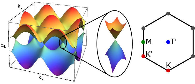
Figure 1: Left: Electronic band structure of the nearest-neighbor tight-binding theory of graphene. Dirac cones around the K-points are enlarged. Right: The first Brillouin zone and terminology for special points therein.

When the Fermi level is shifted across the saddle points by a chemical potential, a change of the topology of the Fermi surface (which is one-dimensional for a 2D crystal) takes place. The distinct circular Fermi (isofrequency) lines surrounding the Dirac points are deformed into triangles when the saddle point is approached, meet to form one large connected region and then break up again into circles around the $\Gamma$-points (see Fig. 2). This is known as neck-disrupting Lifshitz transition Lifshitz:1960su .

The Lifshitz transition is not a true phase transition in the thermodynamic sense (as it is purely topological and not associated with any type of spontaneous symmetry breaking i.e. formation of an ordered phase), but exhibits features commonly associated with such: singularities in free energy and susceptibility at zero temperature with the chemical potential as the control parameter. Unlike phase transitions these singularities are logarithmic (in two dimensions) and not due to interactions but to the vanishing group velocity of electronic excitations at the saddle points which leads to a logarithmic divergence in the density of states (DOS) with increasing surface area of the graphene sheet. This is known as a van Hove singularity (VHS) VanHove:1953kkj and can be observed in a pure form, for instance, in microwave photonic crystals with a Dirac spectrum as macroscopic models for the non-interacting graphene band structure Dietz:2013sga ; Dietz:2016aj and fullerenes with an Atiyah-Singer index theorem Dietz:2015cna .

The fate of the VHS of monolayer graphene in the presence of many-body interactions is a topic of active research. Since interactions are strongly enhanced by the divergent DOS, it is generally believed that the VHS is unstable towards formation of electronic ordered phases. This would imply that the Lifshitz transition becomes a true phase transition in a realistic description of the interacting system at sufficiently low temperatures. It is known that superconductivity can arise from purely repulsive interactions through the Kohn-Luttinger mechanism Kohn:1965ss . Furthermore, it is known that VHSs exist close to the Fermi level in most high-$T_{c}$ superconducting cuprates, so it has long been discussed whether they produce superconducting instabilities generically (known as the “van Hove scenario” Markiewicz:1997zh ). This scenario was also proposed for doped graphene Bostwick:2010as . An exciting possibility specific to graphene furthermore is the emergence of an anomalous time-reversal symmetry violating chiral d-wave superconducting phase from electron-electron repulsion close to the VHS Gonzalez:2008hn ; Chubukov:2012as ; PhysRevB.86.020507 ; Kagan:2014gf ; Schaffer:2014sd ; Loethman:2014gg ; Wang:2012as .

The theoretical perspective is not unambiguous, however. The underlying reason is that several competing channels exist for interaction-driven instabilities at the VHS, and that a subtle interplay of different mechanisms (nesting of the Fermi surface and deviations thereof, relative interaction strengths of couplings at different distances, accounting for electron-phonon interactions etc.) can tilt the balance towards one phase or another. Aside from d-wave superconductivity different formalisms have, for example, predicted superconductivity with pairing in a channel of f-wave symmetry Gonzalez:2013op , spin-density wave (SDW) phases Makogon:2011da , a Pomeranchuk instability Valenzuela:2008fa ; Lamas:2009cv or a Kekulé superconducting pattern Faye:2016xx . And this is by no means an exhaustive list.

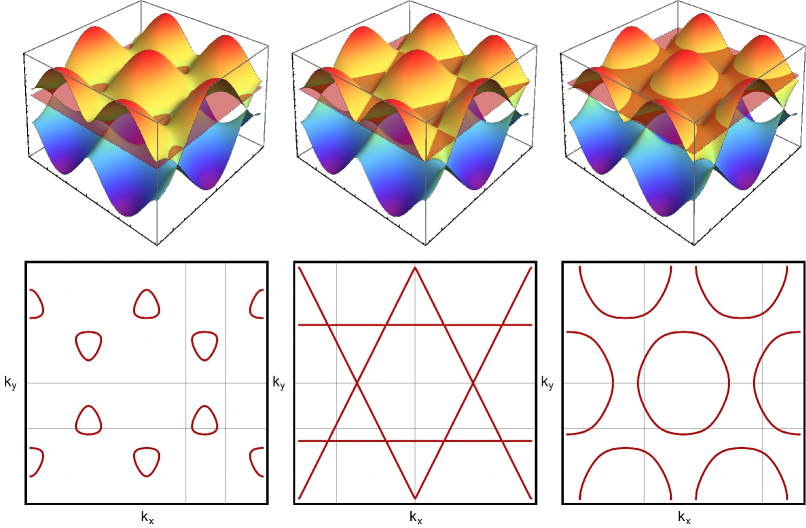
Figure 2: Topology of the Fermi lines (intersection lines with horizontal planes) for Fermi levels below (left), exactly at (middle) and above (right) the saddle points.

On the experimental side, by now there exist several techniques to shift the Fermi level of graphene to the van Hove singularity: The VHS can be probed in systems where gold nanoclusters are intercalated between monolayer graphene and epitaxal graphene Cranney:2010ad , by chemical doping McChesney:2007uh ; Bostwick:2010as , by gating Novoselov:2005df ; Zhang:2005ff ; Efetov:2010sb or in “twisted graphene” Li:2010sd (stacked graphene layers with a rotation angle). Furthermore the valence and conduction bands of graphene can be precisely mapped using angle resolved photoemission spectroscopy (ARPES). Such experiments show clear evidence for a reshaping of the graphene bands by many-body interactions Bostwick200763 and for a warping of the Fermi surface, leading to an extended, not pointlike, van Hove singularity (EVHS) characterized by the flatness of the bands, i.e. lack of energy dispersion, along one direction Bostwick:2010as . ARPES experiments on many different doped graphene systems have also shown bandwidth renormalizations with deviations of several $100$ meV from single-particle band models Ulstrup:2016ha and a massive enhancement of the electron-phonon coupling at the VHS McChesney:2007uh . Unambiguously distinguishing different electronic phases close to the VHS however is an open experimental challenge.

In this work, results of Hybrid-Monte-Carlo (HMC) simulations of the interacting tight-binding theory of graphene are presented. These simulations were carried out at finite chemical potential for spin rather than charge density, as induced by a spin-staggered chemical potential. Although the effects of the two are substantially different, both kinds of chemical potential can be used to tune Fermi levels across the entire range of the $\pi$-bands, including the VHS. The only difference, however substantial, is that the spin-staggered chemical potential shifts the Fermi levels of the two spin orientations in opposite directions corresponding to the pure Zeeman splitting of an in-plane magnetic field Aleiner:2007va .

Technically this modification is necessary to avoid the fermion-sign problem which otherwise arises from the complex phase of the fermion determinant in the charge-doped system, and which causes importance sampling to break down. The system with spin-staggered chemical potential may be viewed as the so-called “phase-quenched” version (defined by the modulus of the fermion determinant in the measure) of graphene at finite charge density. Because the two spin components of the $\pi$-band electrons in graphene correspond to two different fermion flavors, this is entirely analogous to simulating two-flavor QCD at finite isospin density with pion condensation rather than finite baryon density in the form of self-bound nuclear matter which is equally impossible due to a strong sign problem. The phases are clearly distinct but many important questions and genuine finite-density effects in lattice simulations can be addressed at finite isospin density as well.

The particular questions addressed here are about the genuine effects of inter-electron interactions on the VHS and the Lifshitz transition in graphene. Our main focus thereby is the behavior of susceptibilities to identify signatures of instabilities and phase transitions. To directly study the interaction-driven instabilities that might occur in the charge-doped systems described above would require us to measure the particle-hole susceptibility at finite charge density which is however not possible due to the sign problem. We therefore simulate at finite spin density and measure the susceptibility corresponding to ferromagnetic spin-density fluctuations instead which does not have this problem. In the non-interacting limit the two agree, and either one may be used to characterize the electronic Lifshitz transition. Because the spin-staggered chemical potential used here could at least in principle be realized in experiment as well, by sufficiently strong in-plane magnetic fields, our study might also become relevant in its own right in the future.

We chose a realistic microscopic inter-electron interaction potential which accounts for screening by electrons in the $\sigma$-bands Wehling:2011df . A range of different system sizes and temperatures were considered (these are temperatures of the electron gas only, as our simulations presently do not account for phonons). Furthermore, the inter-electron interaction potential was rescaled to different magnitudes, ranging from zero to the full interaction strength of suspended graphene.

The purpose of this work is two-fold: First we wish to assess whether the effects of interactions on the VHS at finite spin density can at least qualitatively be compared with the observations from ARPES data at finite charge density. To this end, we study the reshaping of the $\pi$-bands of the interacting system (with respect to a “flattening” scenario). Secondly, we want to exemplify how the logarithmic divergence of a susceptibility at the VHS in the $T\to 0$ limit can change to a critical scaling law at non-zero $T_{c}$ in the presence of inter-electron interactions, as this would signal the existence of an electronic ordered state close to the VHS and indicate that the Lifshitz transition becomes a true quantum phase transition (with $\mu$ as a control parameter) below this $T_{c}$. Identifying the precise nature of the ordered phase will of course depend on the choice of chemical potential and is thus beyond the scope of this work, however.

This paper is structured as follows: In the following chapter we discuss the behavior of the particle-hole susceptibility in the non-interacting tight-binding theory with temperature and system size where it agrees with that of the ferromagnetic spin-density fluctuations. Exact results for the non-interacting system will serve as a baseline for our studies of the effects of inter-electron interactions. As the HMC method necessitates the introduction of a non-zero temperature of the electron gas (due to the introduction of a Euclidean time dimension which must be of finite extent) and of finite system size, the derivation accounts for both. Furthermore, we derive the leading temperature dependence at the VHS, of the divergent peak height of the susceptibility, in the infinite volume limit. In Chapter III.1 the Hybrid-Monte-Carlo simulation of the interacting theory is introduced, with emphasis on the fermion-sign problem which arises at finite chemical potential for charge-carrier density. We derive expressions for the ferromagnetic and antiferromagnetic spin-density susceptibilities expressed in terms of the inverse fermion matrix. In Chapter IV results of the HMC calculations are presented. These include detailed studies of the temperature and interaction-dependent behavior of the ferromagnetic susceptibility with particular emphasis on the fate of the VHS. Preliminary results concerning the possibility of spin-density wave order from the corresponding antiferromagnetic susceptibility are also presented. We then provide our summary and conclusions in Chapter V.

II Particle-hole susceptibility and Lifshitz transition

II.1 Non-interacting tight-binding theory

As mentioned in the introduction, in the nearest-neighbor tight-binding description of the $\pi$-bands in graphene, due to particle-hole symmetry the particle-hole susceptibility is independent of the sign of the chemical potential $\mu$. Because this is true independently for both spin components, there is thus no distinction between the susceptibilities for charge and spin fluctuations in the non-interacting case, and both equally reflect the Lifshitz transition at finite charge or spin density. The chemical potential $\mu$ this section can therefore be used for either one interchangeably.

In order to understand the relation between the VHS in the electronic quasi-particle DOS $\rho(\omega)$, the Thomas-Fermi susceptibility $\chi$ and the properties of the neck-disrupting electronic Lifshitz transition, one best starts from the particle-hole polarization function $\Pi(\omega,\vec{p};\mu,T)$ at temperature $T$ and chemical potential $\mu$ for charge-carrier density (with $\mu=0$ at half filling), excitation frequency $\omega$ and momentum $\vec{p}$.

The particle-hole polarization function determines the charge-density correlations corresponding to the diagonal time component of the polarization tensor in QED. Using the imaginary-time formalism and subsequent analytic continuation with the appropriate boundary conditions for retarded Green’s functions, at one-loop one arrives at the expression,

$$\Pi(\omega,\vec{p};\mu,T)= -\int_{\mathrm{BZ}}\frac{d^{2}k}{(2\pi)^{2}}\sum_{s,s^{\prime}=\pm 1}$$ (1)

$$\hskip-28.45274pt\frac{g_{\sigma}}{2}\bigg{(}1+ss^{\prime}\frac{{\rm Re}\,\big{(}\phi^{*}_{\vec{k}}\,\phi_{\vec{k}+\vec{p}}\big{)}}{|\phi_{\vec{k}}||\phi_{\vec{k}+\vec{p}}|}\bigg{)}$$

$$\times\frac{n_{f}\big{(}\beta(s^{\prime}\epsilon_{\vec{k}+\vec{p}}-\mu)\big{)}-n_{f}\big{(}\beta(s\epsilon_{\vec{k}}-\mu)\big{)}}{s^{\prime}\epsilon_{\vec{k}+\vec{p}}-s\epsilon_{\vec{k}}-\omega-i\epsilon}\,,$$

where $g_{\sigma}=2$ here for the spin degeneracy, $\phi_{\vec{k}}=\sum_{n}e^{i\vec{k}\vec{\delta}_{n}}$ is the structure factor with nearest-neighbor vectors $\vec{\delta}_{n}$, $n=1,2,3$ on the hexagonal lattice, and single-particle energies $\epsilon_{\vec{k}}=\kappa|\phi_{\vec{k}}|$ (where $\kappa$ is the hopping parameter) in Fermi-Dirac distributions $n_{f}(x)=1/(e^{x}+1)$ at $\beta=1/T$.

The particle-hole polarization or Lindhard function $\Pi$ is a sum of terms describing particle-hole excitations within the same band for $s^{\prime}=s$ (intraband), and terms describing interband excitations for $s^{\prime}=-s$. The complete one-loop expressions for intraband and interband transitions have been computed from Eq. (1) in closed analytic form in Refs. Stauber:2010mn ; Dietz:2013sga .

The imaginary parts of $\Pi$ vanish in the limit $\omega\to 0$ which describes static Lindhard screening. In a subsequent long-wavelength limit $\vec{p}\to 0$, to which only interband excitations contribute, one obtains the usual Thomas-Fermi susceptibility,

$$\chi(\mu)=A_{c}\,\lim_{\vec{p}\rightarrow 0}\,\lim_{\omega\rightarrow 0}\Pi(\omega,\vec{p};\mu,T)\,,$$ (2)

here normalized per unit cell of area $A_{c}=3\sqrt{3}a^{2}/2$ with nearest-neighbor distance $a\approx 1.42\text{\AA}$ for the carbon atoms in graphene. It is straightforwardly calculated as

$$\chi(\mu)= \frac{g_{\sigma}A_{c}}{4T}\int_{\mathrm{BZ}}\frac{d^{2}k}{(2\pi)^{2}}$$ (3)

$$\times\left[\text{sech}^{2}\left(\frac{\epsilon_{\vec{k}}-\mu}{2T}\right)+\text{sech}^{2}\left(\frac{\epsilon_{\vec{k}}+\mu}{2T}\right)\right]~{}.$$

With the present normalization, the zero-temperature limit of $\chi(\mu)$ then in turn agrees with the density of states per unit cell $\rho(\epsilon)$ at the Fermi level $\epsilon=\mu$, i.e.

$$\lim_{T\to 0}\,\chi(\mu)=g_{\sigma}A_{c}\int_{\mathrm{BZ}}\frac{d^{2}k}{(2\pi)^{2}}\,\delta(\epsilon_{\vec{k}}-|\mu|)\equiv\rho(\mu)~{}.$$ (4)

Fig. 3 demonstrates explicitly how the integrand in (3) encodes the effect of temperature on the susceptibility. The sharp Fermi lines which were shown in the lower row of Fig. 2 are smeared out, since a spread of different energy levels may now be excited. The allowed range becomes narrower as temperature is lowered and concentrates on the Fermi level with $\chi$ approaching the DOS there, for $T\to 0$, cf. Eq. (4).

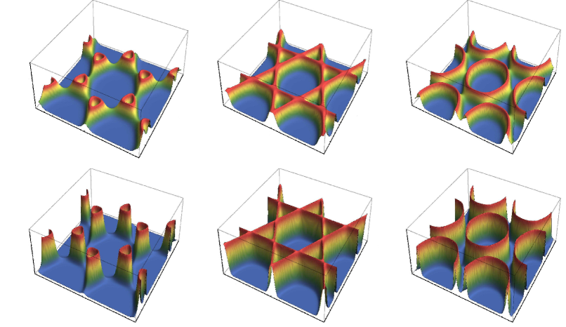
Figure 3: Integrand of Eq. (3) for values of $\mu$ below (right), at (middle) and above (left) the van Hove singularity; from the top to the bottom row the temperature has been lowered by a factor $1/2$ (from $T=\kappa/2$ to $\kappa/4$).

The density of states was first derived for transverse vibrations of a hexagonal lattice by Hobson and Nierenberg in 1953 Hobson:1953df . They found logarithmic divergences near the saddles of the energy bands, i.e., the van Hove singularities, as well as the zeros now identified with the Dirac points. From the corresponding analytical expression of the hexagonal tight-binding model given in CastroNeto:2009zz , one readily obtains for the fermionic system at finite charge-carrier density, with a Fermi energy near one of the van Hove singularities at $\mu=\pm\kappa$,

$$\rho(\mu)=\frac{3g_{\sigma}}{2\pi^{2}\kappa}\Big{\{}-\frac{1}{2}\ln\Big{(}\frac{|\mu|}{\kappa}-1\Big{)}^{2}+2\ln 2+\mathcal{O}\Big{(}\frac{|\mu|}{\kappa}-1\Big{)}\Big{\}}\,.$$ (5)

The correspondingly diverging zero-temperature susceptibility $\chi$ is due to the infinite degeneracy of ground states of the two-dimensional fermionic system when the Fermi level passes through the van Hove singularity. In the thermodynamic sense this can be considered as a zero temperature transition with control parameter $|\mu|$. To illustrate this one introduces the reduced Fermi-energy parameter $z=(|\mu|-\kappa)/\kappa$ to rewrite (5),

$$\chi(z)=\frac{3g_{\sigma}}{2\pi^{2}\kappa}\Big{(}-\ln|z|+2\ln 2+\mathcal{O}(z)\Big{)}\,.$$ (6)

Unlike the cases of first or second order phase transitions, the susceptibility does not diverge with a power law but logarithmically. This is a manifestation of the neck-disrupting electronic Lifshitz transition in two dimensions Lifshitz:1960su ; Blanter1994 . There is no obvious change in symmetry, the transition is only due to the topology change of the Fermi surface. The singular part of the corresponding thermodynamic grand potential is non-zero on both sides of the transition. The original argument is simple, one expands the single-particle energy around a saddle point at $\kappa$ in suitable coordinates,

$$\epsilon_{\vec{k}}=\kappa+\frac{k_{x}^{2}}{2m_{1}}-\frac{k_{y}^{2}}{2m_{2}}\,,$$ (7)

which gives in Eq. (4) a singular contribution

$$\rho_{s}(z)=-\frac{g_{\sigma}A_{c}}{2\pi^{2}}\,\sqrt{m_{1}m_{2}}\,\ln|z|\,.$$ (8)

For the nearest-neighbor tight-binding model on the hexagonal lattice, one verifies that $\sqrt{m_{1}m_{2}}=1/(\kappa A_{c})$ so that $\rho_{s}(z)=-g_{\sigma}/(2\pi^{2}\kappa)\ln|z|$. With a factor of 3 for the three $M$ points per Brillouin zone this agrees with the leading behavior of the zero-temperature susceptibility in Eq. (6) as it should. One integration over $\kappa z$ then yields the number of states in an interval around the saddle, a second one the corresponding contribution to the grand potential $\Omega$ per unit cell which hence acquires a corresponding singularity Blanter1994

$$\Omega_{\mathrm{sing}}=\frac{3g_{\sigma}\kappa}{2\pi^{2}}\,\frac{z^{2}}{2}\ln|z|\,.$$ (9)

It is symmetric around $z=0$. There is thus no order parameter in the usual sense, but one may discuss this transition in terms of a change in the approximate symmetries of the low-energy excitation spectrum with some analogy in excited-state quantum phase transitions Dietz:2013sga .

At any rate, the logarithmic singularity of the electronic Lifshitz transition in the grand potential is restricted to strictly zero temperature. To see this explicitly, we first use the density of states to express the finite-temperature susceptibility in the following form,

$$\chi(\mu)= \frac{1}{4T}\int_{0}^{3\kappa}d\epsilon\,\rho(\epsilon)\,$$

$$\times\left[\text{sech}^{2}\left(\frac{\epsilon-\mu}{2T}\right)+\text{sech}^{2}\left(\frac{\epsilon+\mu}{2T}\right)\right]~{}.$$ (10)

Assuming $\mu>0$ for now, we may drop the second term in the brackets for sufficiently low temperatures, and extend the limits of integration to $\pm\infty$. For the susceptibility maximum at $\mu=\kappa$ we can furthermore approximate $\rho(\epsilon)$ by the expansion in Eq. (5) in the region of support of the integrand around $\epsilon=\kappa$ to obtain,

$$\chi_{\mathrm{max}}=\frac{3g_{\sigma}}{2\pi^{2}\kappa}\Big{\{}-\ln{\big{(}{\pi T}/{\kappa}\big{)}}+\gamma_{E}+3\ln 2+\mathcal{O}(T)\Big{\}}$$ (11)

where $\gamma_{E}$ is the Euler-Mascheroni constant. The maximum of the susceptibility of the electronic Lifshitz transition is finite at finite $T$.

In this way, the logarithmic divergence in the DOS at the VHS is reflected in the Thomas-Fermi susceptibility $\chi(\mu)$. At low but finite temperatures $\chi(\mu)$ peaks when the Fermi level crosses the VHS (for $\mu=\kappa$ in the non-interacting system). The peak height grows logarithmically as temperature is lowered. Its divergence in the zero-temperature limit is a manifestation of the neck-disrupting electronic Lifshitz transition with its logarithmic singularity in the chemical potential as the corresponding control parameter.

So much for the non-interacting and infinite system. Before we discuss finite volume effects and interactions, we can speculate how a reshaping of the saddle points in the single-particle band structure by interactions might qualitatively affect the Lifshitz transition. If we assume a non-Fermi liquid behavior near the saddles for example of the form

$$\epsilon_{\vec{k}}=\epsilon_{0}+\kappa\big{(}c_{1}(k_{x}a)^{\alpha}-c_{2}(k_{y}a)^{\alpha}\big{)}\,,$$ (12)

instead of (7), where we had $\sqrt{c_{1}c_{2}}=3\sqrt{3}/4$, $\epsilon_{0}=\kappa$ and $\alpha=2$ for the non-interacting tight-binding model, we now obtain analogously,

$$\rho_{s}(z)\propto\kappa^{-1}|z|^{-\gamma}\,,\;\;\mbox{with}\;\;\gamma=1-\frac{2}{\alpha}\,.$$ (13)

In Eq. (II.1) this for $\mu=\epsilon_{0}$ then readily yields

$$\chi_{\mathrm{max}}\propto\frac{1}{\kappa}\,\Big{(}\frac{\kappa}{T}\Big{)}^{\gamma}\,,$$ (14)

replacing Eq. (11) for $\gamma\not=0$. We can see that, e.g. for $\alpha=4$ in single-particle energies near the saddles (12), the logarithmic divergence of Eq. (11) turns into a square root divergence of the susceptibility maximum for $T\to 0$ with $\gamma=1/2$. Whereas the limit of a completely flat single-particle energy band with $\alpha\to\infty$ would correspond to $\gamma=1$ and hence $\chi_{\mathrm{max}}\propto 1/T$.

We conclude this section by reiterating that for vanishing two-body interactions, $\chi(\mu)$ is blind to a change of sign. And this is true for each of the spin orientations separately. We will use opposite signs of $\mu$ for the two spin orientations in our simulations below to avoid a fermion-sign problem. While this then corresponds to a Zeeman splitting, as caused by an in-plane magnetic field for example, rather than a change of the charge-carrier density away from half filling, the tight-binding results are unaffected by such a sign change. We may therefore thus use $\chi(\mu)$ with unlike-sign chemical potentials for the two spin states, analogous to isospin chemical potential in Quantum Chromodynamics (QCD), to detect deviations from the pure tight-binding theory in our Hybrid-Monte-Carlo (HMC) simulations, where it can be readily obtained (discussed in Sec. III.3).

To make the comparison between the Lifshitz transition in the non-interacting system and the results from HMC simulations with interactions as direct as possible, in the next subsection we first derive semi-analytic expression for $\chi(\mu)$ in the tight-binding model on finite lattices with the same boundary conditions that we use in the simulations.

II.2 Finite lattices

In our HMC simulations we study graphene sheets of finite surface area, with periodic boundary conditions along the primitive vectors $\vec{a}_{1,2}=\frac{a}{2}(\sqrt{3},\pm 3)$ (where $a\approx 1.42\text{\AA}$ is the inter-atomic distance on the hexagonal lattice) spanning one of the triangular sub-lattices (“Born-von Karman boundary conditions”). We simulate symmetric lattices, with $N$ unit cells along each axis. To take finite size into account, Eq. (3) is rewritten as a sum over the allowed momentum states, which are given by the Laue condition $e^{i\vec{k}\vec{R}}=1$, where $\vec{R}=n\vec{a}_{1}+m\vec{a}_{2}$ with $n,m\in[1,\cdots,N]$. The momentum states are

$$\vec{k}=\frac{n}{N}\vec{b}_{1}+\frac{m}{N}\vec{b}_{2}~{},$$ (15)

where $\vec{b}_{1,2}=\frac{2\pi}{3a}(\sqrt{3},\pm 1)$ are the the base vectors of the reciprocal lattice. The integral measure $d^{2}k$ turns into a finite surface element $(\Delta k)^{2}=|\vec{b}_{1}\times\vec{b}_{2}|/N^{2}=A_{\mathrm{BZ}}/N^{2}$, where $A_{\mathrm{BZ}}=(2\pi)^{2}/A_{c}$ is the area of the first Brillouin zone, and the integral in Eq. (3) for the susceptibility of a finite sheet becomes,

$$\chi(\mu)=\frac{g_{\sigma}}{4TN^{2}}\sum_{n,m} \left[\text{sech}^{2}\left(\frac{\epsilon_{mn}-\mu}{2T}\right)\right.$$

$$\hskip 28.45274pt\left.+\,\text{sech}^{2}\left(\frac{\epsilon_{mn}+\mu}{2T}\right)\right]~{}.$$ (16)

Here $\epsilon_{mn}$ is the dispersion relation, evaluated at the points defined by Eq. (15):

$$\epsilon_{mn}=\kappa\left\{3+4\cos{\left(\pi\frac{n+m}{N}\right)}\cos{\left(\pi\frac{n-m}{N}\right)}\right.$$

$$\left.+2\cos{\left(2\pi\frac{n+m}{N}\right)}\right\}^{\frac{1}{2}}~{}.$$ (17)

Eq. (II.2) is of a form which can be compared directly to the simulations. The sums cannot be carried out analytically, but are straightforward to evaluate numerically.

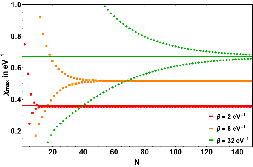
Figure 4: Finite-size scaling of the susceptibility peak at different temperatures ($\beta=1/T$) from Eq. (II.2); the horizontal lines indicate the leading-order prediction from Eq. (11), the slight deviations of the infinite volume limit from this prediction for $\beta=2$ eV^-1 are due to $\mathcal{O}(T)$ corrections.

Of course there is no divergence of the particle-hole susceptibility in a finite volume, not even at zero temperature. The spectrum is discrete and the total number of states is finite, so the density of states cannot diverge either. In Ref. Dietz:2013sga it was shown, however, that the finite-size scaling of the susceptibility maximum at $T=0$ is logarithmic likewise, namely

$$\chi_{\mathrm{max}}=\frac{3g_{\sigma}}{2\pi^{2}\kappa}\,\Big{(}\ln N_{c}-2\ln\pi+1+{\cal O}(1/N_{c})\Big{)}\,,$$ (18)

where $N_{c}=N^{2}$ is the number of unit cells. Since our simulations are carried out at finite temperature, it is clear that we cannot observe this behavior directly because it is valid only at strictly zero temperature. The extension of the analytic expressions to finite volume and finite temperature is not so straightforward, however, and cannot be done analytically.

Therefore, we use the implicit representation of $\chi(\mu)$ for a finite sheet at temperature $T$ in Eq. (II.2) and compute the sums numerically. The results of $\chi$ at $\mu=\kappa$ are shown for various lattice sizes and temperatures in Fig. 4. In general, for any finite temperature, $\chi(\mu=\kappa,N)$ for $N\to\infty$ approaches a flat asymptote $\propto\ln(\beta\kappa)$ which in turn increases with $\beta=1/T$ according to Eq. (11). It is the temperature dependence of these asymptotic values which follows Eq. (11). Convergence to the infinite volume limit becomes slower for decreasing temperatures as the asymptotic value increases.

Fig. 4 shows a strong influence of the parity of the lattice, where odd lattices approach the $N\to\infty$ limit from below and even lattices from above. For a fixed lattice size, the peak height either diverges (for even lattices) or goes to zero (for odd lattices) as $T\to 0$. This difference arises from the fact that the sums in Eq. (II.2) only contain momentum modes which hit the M-points exactly when $N$ is even. For even $N$, points on the lines with $\text{sech}^{2}((\epsilon_{mn}-\mu)/2T)=1$ contribute with diverging weight $\propto 1/T$ to the sum (cf. Fig. 3), while for odd $N$ there are no such points but only points that cluster around these lines when the system becomes large.

III Inter-electron interactions

III.1 Simulation setup

The present work implements Hybrid-Monte-Carlo simulations of the interacting tight-binding theory on the hexagonal graphene lattice, based on a formalism developed by Brower et al. Brower:2012zd ; Brower:2012ze , which goes beyond the low-energy approximation (studied extensively in the past Drut:2008rg ; Drut:2009gg ; Drut:2009rf ; Drut:2010ff ; Drut:2011fd ; Hands:2008dg ; Armour:2009vj ; Armour:2011ff ; Buividovich:2012uk ; Giedt:2011df ) and is thus able to capture the full band structure beyond the Dirac cones. The HMC method on the graphene lattice is by now well established, and has been successfully applied in conclusive studies of the antiferromagnetic phase transition Buividovich:2012nx ; Ulybyshev:2013swa ; Smith:2013pxa ; Smith:2014tha ; Smith:2014vta as well as in ongoing studies of the phase diagram of an extended fermionic Hubbard model on the hexagonal graphene lattice Buividovich:2016tgo . Numerous other topics were also addressed with HMC, such as the optical conductivity of graphene Boyda:2016emg , the effect of hydrogen adatoms Ulybyshev:2015opa ; Buividovich:2017sju or the single quasi-particle spectrum of carbon nanotubes Luu:2015gpl .

We have written about our setup in great detail in the past (see ref. Smith:2014tha for a step-by-step derivation) and will only provide a summary here. In particular, we focus on the additional challenges which arise when introducing a chemical potential (i.e. the fermion-sign problem) and discuss our workaround solution (a spin-dependent sign flip). To be clear: This work does not attempt to solve the sign-problem, but rather studies a modified Hamiltonian which is free of such a problem. To assess to what degree the physics is changed by this modification is part of the motivation for this work.

The starting point is the interacting tight-binding Hamiltonian in second-quantized form

$$H= \sum_{\langle x,y\rangle}(-\kappa)(a_{x}^{\dagger}a_{y}+b_{x}^{\dagger}b_{y}+\textrm{h.c.})$$

$$+\sum_{x,y}\,q_{x}V_{xy}q_{y}+\sum_{x}m_{s}(a_{x}^{\dagger}a_{x}+b_{x}^{\dagger}b_{x})~{}.$$ (19)

The chemical potential is absent at this stage and will be introduced later. The first sum in Eq. (19) runs over pairs of nearest neighbors only (with a hopping parameter $\kappa=2.7$ eV), so we neglect higher order hoppings. The other sums run over all sites (including both sublattices) of the $2D$ hexagonal lattice. Here $a_{x}^{\dagger},a_{x}$ denote creation/annihilation operators for electrons in the $\pi$-bands with spin $+1/2$ in the $z$-direction (perpendicular to the graphene sheet) and $b_{x}^{\dagger},b_{x}$ are analogous operators for holes (“anti-particles”) with spin $-1/2$. The hopping term also contains a sublattice dependent sign-flip for the $b_{x}^{\dagger},b_{x}$ operators Smith:2014tha .

We have also added in Eq. (19) a staggered mass term $m_{s}=(-1)^{s}\,m$ with a sublattice $s=0,1$ dependent sign to regulate the low-lying eigenvalues of the Hamiltonian, as is customary in lattice-QCD simulations. While simulations at exactly zero mass are possible in principle Buividovich:2016tgo (unlike lattice QCD there appear to be no topological obstructions to simulating at exactly zero mass here), a finite mass term has numerical advantages, and it only affects the low-lying excitations around the Dirac points which are not the primary focus of our present study. In fact, our investigation of the Lifshitz transition turns out to be rather insensitive to this mass term as one might expect, based on the band structure of the non-interacting system, as long as $m_{s}\ll\kappa$. Moreover, a spin and sublattice-staggered mass term of this form also serves as an external field for sublattice-symmetry breaking by spin-density wave formation. So derivatives with respect to $m_{s}$ may be used to detect an instability of the ground state towards SDW order.

The operator $q_{x}=a_{x}^{\dagger}a_{x}-b_{x}^{\dagger}b_{x}$ represents physical charge. Interactions are taken to be instantaneous, which is true to good approximation since $v_{F}\ll c$, where $v_{F}$ is the Fermi velocity of the electrons. One of the great advantages of the instantaneous Hamiltonian in Eq. (19) (compared to implementing the photon as an Abelian gauge field on link variables) is that any positive-definite matrix can be chosen for $V_{xy}$, leaving a great freedom to choose a realistic two-body potential to describe microscopic interactions. In particular, it is possible to implement deviations from pure Coulomb-type interactions due to screening from $\sigma$-band and other localized electrons.

In this work, we choose a two-body potential which accounts for precisely this screening as obtained from calculations within a constrained random-phase approximation (cRPA) by Wehling et al. in Ref. Wehling:2011df . Therein exact values were obtained for the on-site $U_{00}$, nearest-neighbor $U_{01}$, next-nearest-neighbor $U_{02}$, and third-nearest-neighbor $U_{03}$ interaction parameters, and a momentum dependent phenomenological dielectric screening formula derived, based on a thin-film model, which can be used to interpolate to an unscreened Coulomb tail at long distances. Here we use the “partially screened Coulomb potential” of Ref. Smith:2014tha which combines both results via a parametrization based on a distance dependent Debye mass $m_{D}$. The matrix elements $V_{xy}$ are then filled using

$$V(r)=\left\{\begin{array}[]{lr}U_{00},U_{01},U_{02},U_{03}&,\;r\leq 2a\\[2.0pt] e^{2}\left(c\,\displaystyle\frac{\exp(-m_{D}r)}{a(r/a)^{\gamma}}+m_{0}\right)&,\;r>2a\end{array}\right.$$ (20)

where $a$ is the nearest-neighbor distance as before, and $m_{D}$, $m_{0}$, $c$ and $\gamma$ are piecewise constant chosen such that $m_{D},m_{0}\to 0$ and $c,\gamma\to 1$ for $r\gg a$. For the precise values of these parameters we refer to the tables in Smith:2014tha . The resulting interaction potential is shown in comparison to the unscreened Coulomb potential in Fig. 5.

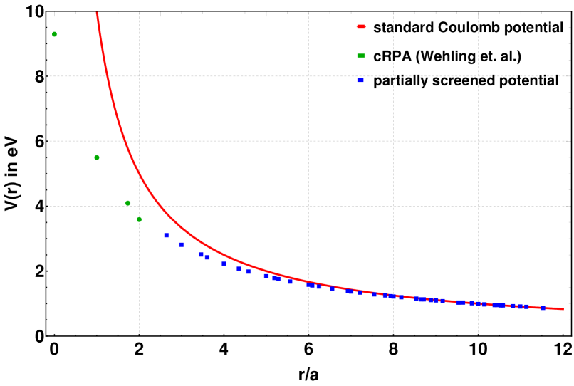
Figure 5: Comparison of the standard Coulomb potential (red) with the partially screened potential given by Eq. (20). The first four points are exact cRPA results of Ref. Wehling:2011df (green), while the remaining ones are obtained from the interpolation based on the thin-film model from the same reference (blue).

We note in passing that there is still some theoretical uncertainty concerning the screening effects generated by the $\sigma$-band electrons at short distances (for a detailed discussion, see Ref. Tang:2015as ). For the purpose of our present study, this is of minor importance because our main conclusions should be insensitive to small variations of the short-range interaction parameters. Larger variations of these parameters on the other hand can lead to very rich phase diagrams including topological insulating phases Raghu:2008a . A detailed study of competing order from HMC simulations of the extended Hubbard model on the hexagonal lattice with varying on-site and nearest-neighbor couplings currently in progress Buividovich:2016tgo .

To proceed, one derives a functional-integral formulation of the grand-canonical partition function $Z={\rm Tr}\,e^{-\beta H}$, in which the ladder-operators are replaced by Grassman valued fermionic field variables, by factorizing $e^{-\beta H}$ into $N_{t}$ terms (taken to be “slices” in Euclidean time) and inserting complete sets of fermionic coherent states. Formally, $N_{t}$ must be taken to infinity to obtain an exact result, but for numerical simulations $N_{t}$ is a finite number. This implies a discretization error of order O($\delta^{2}$), where $\delta=\beta/N_{t}$. The final result is

$$Z =\int\prod_{t=0}^{N_{t}-1}\left[\prod_{x}d\psi^{*}_{x,t}\,d\psi_{x,t}\,d\eta^{*}_{x,t}\,d\eta_{x,t}\right]\exp\Big{\{}-\delta\Big{[}\frac{1}{2}\sum_{x,y}Q_{x,t+1,t}V_{xy}Q_{y,t+1,t}$$

$$-\sum_{\langle x,y\rangle}\kappa(\psi_{x,t+1}^{*}\psi_{y,t}+\psi_{y,t+1}^{*}\psi_{x,t}+\eta_{y,t+1}^{*}\eta_{x,t}+\eta_{x,t+1}^{*}\eta_{y,t})+\sum_{x}m_{s}(\psi_{x,t+1}^{*}\psi_{x,t}+\eta_{x,t+1}^{*}\eta_{x,t})$$

$$+\frac{1}{2}\sum_{x}V_{xx}(\psi_{x,t+1}^{*}\psi_{x,t}+\eta_{x,t+1}^{*}\eta_{x,t})\Big{]}-\sum_{x}\big{[}\psi^{*}_{x,t+1}(\psi_{x,t+1}-\psi_{x,t})+\eta^{*}_{x,t+1}(\eta_{x,t+1}-\eta_{x,t})\big{]}\Big{\}}~{}.$$ (21)

Here we have used the notation $Q_{x,t,t^{\prime}}=\psi_{x,t}^{*}\psi_{x,t^{\prime}}-\eta_{x,t}^{*}\eta_{x,t^{\prime}}$.

One would now like to integrate out the fermionic fields to obtain an expression containing only determinants of a fermionic matrix $M$, which can then be sampled stochastically. This is prevented by fourth powers of the fields, appearing in the interaction term $\sim q_{x}V_{xy}q_{y}$. These can be removed by a Hubbard-Stratonovich transformation

$$\exp\big{\{} -\frac{\delta}{2}\sum_{x,y}q_{x}V_{xy}q_{y}\big{\}}\propto\int\big{[}\prod_{x}\phi_{x}\big{]}\,$$

$$\times\exp\big{\{}-\frac{\delta}{2}\sum_{x,y}\phi_{x}V_{xy}^{-1}\phi_{y}-i\,\delta\sum_{x}\phi_{x}q_{x}\big{\}}~{},$$ (22)

at the expense of introducing an additional dynamical scalar field $\phi$ (“Hubbard field”). The resulting expression contains only quadratic powers, so Gaussian integration can be carried out, which yields

$$Z=\int\big{[} \prod_{x,t}\phi_{x,t}\big{]}\ \,\det\big{[}M(\phi)M^{\dagger}(\phi)\big{]}$$

$$\times\exp\big{\{}-\frac{\delta}{2}\sum_{t=0}^{N_{t}-1}\sum_{x,y}\phi_{x,t}V_{xy}^{-1}\phi_{y,t}\big{\}}~{},$$ (23)

A subtlety here is that, if the Hubbard-Stratonovich transformation (22) is naively applied to Eq. (21), the determinant of the fermion matrix is a high-degree polynomial of the non-compact field $\phi$ whose numerical evaluation is plagued by uncontrollable rounding errors. It is therefore advantageous to use an alternative fermion discretization with a coupling to a compact Hubbard field Brower:2012zd ; Ulybyshev:2013swa ; Smith:2014tha . Its derivation is slightly more involved but straightforward, essentially based on applying the Hubbard-Stratonovich transformation before introducing the fermionic coherent states. The matrix elements are then computed using the identity

$$\langle\xi|\,e^{\sum_{x,y}a_{x}^{\dagger}A_{xy}a_{y}}\,|\xi^{\prime}\rangle=\exp\left(\sum_{x,y}\xi^{*}_{x}\left(e^{A}\right)_{xy}\xi^{\prime}_{y}\right)~{},$$ (24)

which holds for arbitrary matrices $A$. Here, $A$ is a diagonal matrix with elements $A_{xx}=\pm i\delta\,\phi_{x}$. The differences are of subleading order $\delta^{2}$ in the time discretization. Hence both are equivalent at the order $\delta$ and share the same continuum limit. It is this modified version of the fermion matrix $M(\phi)$, with the compact Hubbard field, which is used for numerically stablility in our simulations. Its matrix elements are given by (for details, see Ref. Smith:2014tha ):

$$M_{(x,t)(y,t^{\prime})}(\phi)=\delta_{xy}(\delta_{tt^{\prime}}-e^{-i\frac{\beta}{N_{t}}\phi_{x,t}}\delta_{t-1,t^{\prime}})$$

$$\quad-\kappa\frac{\beta}{N_{t}}\sum\limits_{n}\delta_{y,x+\vec{\delta}_{n}}\delta_{t-1,t^{\prime}}+m_{s}\frac{\beta}{N_{t}}\delta_{xy}\delta_{t-1,t^{\prime}}~{}.$$ (25)

The matrix contains terms corresponding to the different contributions from the tight-binding Hamiltonian and a covariant derivative in Euclidean time, in which the Hubbard field enters in form of a gauge connection where $\phi$ acts as an electrostatic potential.

Both $M$ and $M^{\dagger}$ appear in Eq. (23) due to the two spin orientations entering as independent degrees of freedom into the Hamiltonian (we are essentially treating spin-up and spin-down states as different particle flavors). The resulting expression is suitable for simulation via HMC at half filling ($\mu=0$), as the integrand may be interpreted as a weight function for the Hubbard field $\phi$.

III.2 Hybrid-Monte-Carlo and the fermion-sign problem

The HMC method (originally developed for strongly interacting fermionic quantum field theories Duane:1987de ) consists in essence of creating a distribution of field configurations representative of the thermal equilibrium, by evolving the $\phi$ field in computer time $\tau$ through a fictitious deterministic dynamical process, governed by a conserved classical Hamiltonian defined in the higher dimensional space spanned by real Euclidean space-time and $\tau$. Quantum fluctuations enter in the form of stochastic refreshments of the canonical momentum $\pi$ associated with the Hubbard field $\phi$. As a symplectic integrator must be used to solve Hamilton’s equations for $\phi$ and $\pi$, an additional error arises from the finite step-size of this integrator, which is subsequently corrected by a Metropolis accept/reject step. HMC is thus an exact algorithm (see Ref. Smith:2014tha for further details).

HMC is a form of importance sampling, i.e. a method of approximating the functional integral by probabilistically generating points in configuration space which are clustered in the regions that contribute most to the integral. A crucial criterion for its applicability is the existence of a real and positive-definite measure for the dynamical fields, which may then be interpreted as a probability density. This is true here only because the phases of $M$ and $M^{\dagger}$ cancel exactly in Eq. (23). As we will see, this no longer holds at non-zero charge density.

To generate finite charge-carrier density, one would have to add a corresponding chemical potential $\mu$, replacing the Hamiltonian in Eq. (19) by

$$H\to H-\mu\sum_{x}q_{x}=H-\mu\sum_{x}(a_{x}^{\dagger}a_{x}-b_{x}^{\dagger}b_{x})\,.$$ (26)

At the level of the partition function, this leads to the modification

$$Z(\mu)=\int\prod_{t=0}^{N_{t}-1}\left[\prod_{x}d\psi^{*}_{x,t}\,d\psi_{x,t}\,d\eta^{*}_{x,t}\,d\eta_{x,t}\right]$$

$$~{}\times\exp\Big{\{}\left(\ldots\right)+\frac{\beta\mu}{N_{t}}\sum_{x}(\psi_{x,t+1}^{*}\psi_{x,t}-\eta_{x,t+1}^{*}\eta_{x,t})\Big{\}}~{}.$$ (27)

After integrating out the fermion fields, one obtains a modified version of Eq. (23)

$$Z= \int\big{[}\prod_{x,t}\phi_{x,t}\big{]}\ \,\det\big{[}M(\phi,\mu)\widetilde{M}(\phi,\mu)\big{]}$$

$$\times\exp\big{\{}-\frac{\delta}{2}\sum_{t=0}^{N_{t}-1}\sum_{x,y}\phi_{x,t}V_{xy}^{-1}\phi_{y,t}\big{\}}~{},$$ (28)

where

$$M(\phi,\mu)_{(x,t)(y,t^{\prime})}= M(\phi,0)_{(x,t)(y,t^{\prime})}-\mu\frac{\beta}{N_{t}}\delta_{xy}\delta_{t-1,t^{\prime}}~{},$$

$$\widetilde{M}(\phi,\mu)_{(x,t)(y,t^{\prime})}= M^{\dagger}(\phi,0)_{(x,t)(y,t^{\prime})}+\mu\frac{\beta}{N_{t}}\delta_{xy}\delta_{t-1,t^{\prime}}$$

$$= M^{\dagger}(\phi,-\mu)_{(x,t)(y,t^{\prime})}~{}.$$ (29)

There is no cancellation of phases in Eq. (28), thus importance sampling breaks down, as we no longer can interpret the integrand as the weight of a given microstate in the ensemble. This is at the root of the fermion-sign problem. Whether it is a hard problem or not depends on the expectation value of the phase of the determinant in the “phase-quenched” theory defined by the modulus of the fermion determinant in the measure, i.e. writing

$$Z= \int\big{[}\prod_{x,t}\phi_{x,t}\big{]}\ \,\big{|}\det M(\phi,\mu)\big{|}^{2}\,\frac{\det\widetilde{M}(\phi,\mu)}{\det\widetilde{M}(\phi,-\mu)}$$

$$\times\exp\big{\{}-\frac{\delta}{2}\sum_{t=0}^{N_{t}-1}\sum_{x,y}\phi_{x,t}V_{xy}^{-1}\phi_{y,t}\big{\}}~{},$$ (30)

we consider the complex ratio of determinants with opposite-sign chemical potentials as an observable in the phase-quenched theory with partition function $Z_{\mathrm{pq}}$ and

$$\frac{Z(\mu)}{Z_{\mathrm{pq}}(\mu)}\,=\,\Big{\langle}\frac{\det\widetilde{M}(\phi,\mu)}{\det\widetilde{M}(\phi,-\mu)}\Big{\rangle}_{\mathrm{pq}}\,.$$ (31)

Obviously this ratio is unity at half filling (i.e. for $\mu\to 0$) and at vanishing interaction strength for all $\mu$, because the non-interacting tight-binding theory is blind to the sign of $\mu$ for each spin component individually.

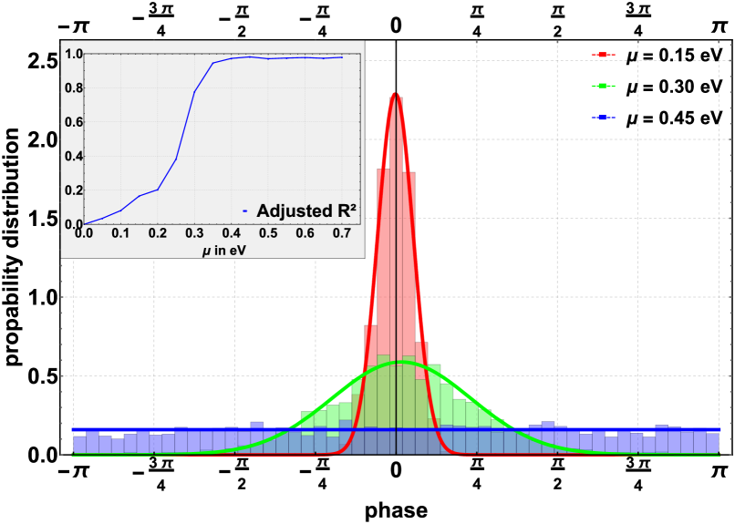
Figure 6: Histograms of the phase of $\det\widetilde{M}(\phi,\mu)/\det\widetilde{M}(\phi,-\mu)$ obtained from a $6\times 6$ lattice at $\beta=2\textrm{ eV}^{-1}$ for different $\mu$, at $10\,\%$ of the interaction strength of suspended graphene. The results are modelled with gaussian ($\mu=0.15\textrm{ eV}^{-1}$ and $0.30\textrm{ eV}^{-1}$) and uniform ($\mu=0.45\textrm{ eV}^{-1}$) distributions respectively. The inlay shows the adjusted $\textrm{R}^{2}$ for fitting a constant to the data at a range of different $\mu$. For $\mu\gtrsim 0.4\textrm{ eV}$ the numerical datais well described by a uniform distribution, indicating a hard sign problem.

To exemplify that the signal is indeed lost quickly, however, when the chemical potential for charge-carrier density is tuned away from half filling in the interacting theory, we have measured the modulus and the complex phase of the ratio of determinants in Eq. (31) on a $6\times 6$ lattice, at $\beta=2\,\textrm{eV}^{-1}$ and $10\,\%$ of the interaction strength of suspended graphene. This method of “reweighting” therefore certainly fails near the van Hove singularity, already at rather moderate interaction strengths. Fig. 6 shows histograms of the phase for different values of $\mu$ together with fit-model curves. As a measure for the signal-to-noise ratio we have used the adjusted $R^{2}$ associated with attempting to model the histograms with a uniform distribution (this quantity is $0$ for a strictly non-linear relation between the data and the fitted curve and $1$ for a perfect linear dependence). As one can see in the figure, the adjusted $R^{2}$ of the constant fit shows a rather rapid crossover and approaches values close to $1$ at $\mu\approx 0.4\textrm{eV}$ which indicates that the signal is lost in the noise already on the $6\times 6$ lattice. The effect will be further enhanced with increasing lattice sizes. Note that the modulus of the ratio of determinants is not unity here eihter. In fact, it also decreases with $\mu$. As usual, however, it is the phase fluctuations that are primarily responsible for the loss of signal due to cancellations.

The underlying physical reason for a non-polynomially hard signal-to-noise-ratio problem typically is that the overlap of phase-quenched and full ensembles tends to zero exponentially because of a complete decoupling of the corresponding Hilbert spaces in the infinite-volume limit when the two ensembles correspond to excitations above different finite-density ground states (here charge-carrier versus spin density). An exponential error reduction might be possible with generalized density-of-states methods Langfeld:2012ah which work beautifully in spin systems Langfeld:2014nta and heavy-dense QCD Garron:2016noc but have yet to be applied to strongly interacting theories with dynamical fermions.

Dense fermionic theories with a sign problem are a very active field of research and we cannot cover the vast body of literature here. There is no general solution, however.

Sometimes cluster algorithms Chandrasekharan:1999cm or extensions thereof that exploit cancellations of field configurations Huffman:2013mla help. On the other hand, when they do, there also appears to be an underlying Majorana positivity Li:2015a ; Wei:2016a ; Li:2016a and the theory therefore really is sign-problem free as in the case of the anti-unitary symmetries such as time-reversal invariance with Kramers degeneracy discussed below.

Sometimes it is possible to simulate dual theories with worm algorithms Prokofev:2001ddj ; Mercado:2013ola . Deformation of the originally real configuration space into a complex domain can help by either sampling Lefschetz thimbles of constant phase Mukherjee:2014hsa , reducing the sign problem to that of the residual phases, or more generally, field manifolds with a milder sign problem obtained from holomorphic gradient flow Alexandru:2016ejd . Doubling the number of degrees of freedom by complexification one can also try a complex version of stochastic quantization, i.e. by simulating the corresponding Complex Langevin process Sexty:2014dxa .

While all these techniques have their difficulties and are actively being further developed, in the mean time we follow a different strategy here. This is to simulate a sign-problem free variant of the original theory with standard Monte-Carlo techniques and study genuine finite-density effects where importance sampling is possible. Such variants could be theories with anti-unitary symmetries such as two-color QCD, with two instead of the usual three colors Boz:2015ppa ; Holicki:2017psk , or $G_{2}$-QCD, with the exceptional Lie group $G_{2}$ replacing the $SU(3)$ gauge group of QCD Maas:2012wr ; Wellegehausen:2015iea .

The arguably simplest variant is the phase-quenched theory itself, however. In two-flavor QCD this amounts to simulating at finite isospin density Detmold:2012wc ; Brandt:2016zdy . Here it corresponds to introducing a chemical potential for finite spin density, like a pure Zeeman term from an in-plane magnetic field, rather than one for finite charge-carrier density, as mentioned above. To this end we add a chemical potential $\mu_{\sigma}=(-1)^{\sigma}\mu$ with a spin $\sigma=0,1$ (for up/down) dependent sign, i.e. instead of (26) we use the replacement

$$H\to H-\mu\sum_{x}(a_{x}^{\dagger}a_{x}+b_{x}^{\dagger}b_{x})~{}.$$ (32)

Compared to (26), the sign of the term $\sim b_{x}^{\dagger}b_{x}$ has been flipped. This leads to a modification of the spin-down determinant in Eq. (29), such that

$$\widetilde{M}(\phi,\mu_{\sigma})_{(x,t)(y,t^{\prime})}= M^{\dagger}(\phi,0)_{(x,t)(y,t^{\prime})}-\mu\frac{\beta}{N_{t}}\delta_{xy}\delta_{t-1,t^{\prime}}$$

$$= M^{\dagger}(\phi,\mu)_{(x,t)(y,t^{\prime})}~{}.$$ (33)

Cancellation of the phases in the partition function is thus restored; $\mu_{\sigma}$ shifts the Fermi surfaces for electron-like and hole-like excitations in opposite directions. As the nearest-neighbor tight-banding bands are symmetric under exchange of particle-like and hole-like states individually for each spin, the Lifshitz transition in the non-interacting theory is in fact blind to this change of sign. As a result, $\mu_{\sigma}$ induces a Zeeman-splitting but without the phase factors from a Peierls substitution in the hopping term. It therefore describes graphene coupled to an in-plane magnetic field Aleiner:2007va . In the following we will omit the spin-index. It is implied that $\mu$ is spin staggered from now on, i.e. corresponding to $\mu_{\sigma}=(-1)^{\sigma}\mu$ as in Eq. (32).

III.3 Observables

Expectation values of physical operators in the thermal ensemble are expressed in the path-integral formalism as

$$\langle O\rangle=\frac{1}{Z}\int D\phi\,O(\phi)\,\text{det}\left(MM^{\dagger}\right)e^{-S(\phi)}~{}.$$ (34)

Their representation in the space of field variables can be obtained from derivatives of the partition function with respect to corresponding source terms. We are interested in the particle-hole susceptibility (2), which up to a factor of $\beta=1/T$ agrees with the number susceptibility (per unit cell). Hence it is given by

$$\chi(\mu) =-\frac{1}{N_{c}}\,\left(\frac{d^{2}\Phi}{d\mu^{2}}\right)$$ (35)

$$=\frac{1}{N_{c}\beta}\left[\frac{1}{Z}\frac{d^{2}Z}{d\mu^{2}}-\frac{1}{Z^{2}}\left(\frac{dZ}{d\mu}\right)^{2}\right]~{},$$

where $\Phi=-T\ln{Z}$ is the grand-canonical potential and $N_{c}=N^{2}$ is the number of unit cells. Using the path-integral representation of $Z$, we can express $\chi(\mu)$ in terms of the fermion matrix $M(\phi)$, since

$$\frac{1}{Z}\frac{d^{n}Z}{d\mu^{n}}=\frac{1}{Z}\int D\phi\left[\frac{d^{n}}{d\mu^{n}}\text{det}\left(MM^{\dagger}\right)\right]e^{-S(\phi)}~{}.$$ (36)

Calculating the derivatives for $n=1,2$ we obtain

$$\frac{d}{d\mu}\text{det}\left(MM^{\dagger}\right)=2\,\text{det}\,\left(MM^{\dagger}\right)\,\text{ReTr}\,\left(M^{-1}\frac{dM}{d\mu}\right)$$ (37)

and

$$\frac{d^{2}}{d\mu^{2}}\text{det} \left(MM^{\dagger}\right)=4\,\text{det}\left(MM^{\dagger}\right)\left\{\left[\text{ReTr}\,\left(M^{-1}\frac{dM}{d\mu}\right)\right]^{2}\right.$$

$$\left.\quad\quad\quad-\frac{1}{2}\,\text{ReTr}\,\left(M^{-1}\frac{dM}{d\mu}M^{-1}\frac{dM}{d\mu}\right)\right\}.$$ (38)

Using these relations we can write the spin-staggered particle-hole susceptibility as $\chi=\chi_{\textrm{con}}+\chi_{\textrm{dis}}$, with

$$\chi_{\textrm{con}}(\mu)= \frac{-2}{N_{c}\beta}\left\langle\text{ReTr}\,\left(M^{-1}\frac{dM}{d\mu}M^{-1}\frac{dM}{d\mu}\right)\right\rangle$$

$$\chi_{\textrm{dis}}(\mu)= \frac{4}{N_{c}\beta}\left\{\left\langle\left[\text{ReTr}\,\left(M^{-1}\frac{dM}{d\mu}\right)\right]^{2}\right\rangle\right.$$

$$\left.-\left\langle\text{ReTr}\,\left(M^{-1}\frac{dM}{d\mu}\right)\right\rangle^{2}\right\}~{},$$ (39)

where $\chi_{\textrm{con/dis}}$ denote the connected and disconnected contributions respectively. The brackets on the right-hand sides of Eqs. (39) are understood as averages over a representative set of field configurations. The traces can be evaluated with noisy estimators.

A susceptibility $\chi^{\textrm{sdw}}$ corresponding to the fluctuations of the antiferromagnetic spin-density wave order parameter computed at half filling in Ref. Buividovich:2016tgo can be obtained in complete analogy to the above, replacing all derivatives with respect to $\mu$ by derivatives with respect to the sublattice-staggered mass $m_{s}=(-1)^{s}\,m$ in Eq. (19). The resulting expressions are then of precisely the same form as Eqs. (39), with the replacement $\mu\to m$,

$$\chi_{\textrm{con}}^{\textrm{sdw}}(\mu)= \frac{-2}{N_{c}\beta}\left\langle\text{ReTr}\,\left(M^{-1}\frac{dM}{dm}M^{-1}\frac{dM}{dm}\right)\right\rangle$$

$$\chi_{\textrm{dis}}^{\textrm{sdw}}(\mu)= \frac{4}{N_{c}\beta}\left\{\left\langle\left[\text{ReTr}\,\left(M^{-1}\frac{dM}{dm}\right)\right]^{2}\right\rangle\right.$$

$$\left.-\left\langle\text{ReTr}\,\left(M^{-1}\frac{dM}{dm}\right)\right\rangle^{2}\right\}~{}.$$ (40)

IV Results

In this chapter we first present our results for the susceptibility $\chi(\mu)$ of ferromagnetic spin-density fluctuations, i.e. the spin-staggered particle-hole susceptibility, from Hybrid-Monte-Carlo simulations of the interacting tight-binding theory at finite spin-density and temperature. Only in the last subsection we briefly come back to the spin-density dependence of the antiferromagnetic SDW susceptibility $\chi^{\textrm{sdw}}$ as well.

All results were obtained from hexagonal lattices of finite size with periodic Born-von Kármán boundary conditions, with an equal number of unit cells in each principal direction. We chose a sublattice and spin-staggered mass $m_{s}$ of magnitude $m=0.5\textrm{ eV}$, an inter-atomic spacing of $a=1.42\text{ \AA}$ and a hopping parameter of $\kappa=2.7\textrm{ eV}$. We furthermore use the partially screened Coulomb potential discussed in detail in Section III.1 and Ref. Smith:2014tha .

The rescaled effective interaction strength $\alpha_{\textrm{eff}}$ is defined in the following as $\alpha_{\textrm{eff}}=\lambda\cdot\alpha_{\textrm{graphene}}$ with $\alpha_{\textrm{graphene}}=\frac{e^{2}}{\hbar v_{F}}\approx 2.2$ ($\lambda$ thus acts as a global rescaling factor which changes each element of the interaction matrix in the same way, i.e. $V_{xy}\to\lambda V_{xy}$). Interactions were rescaled to different magnitudes in the range $\lambda=[0,1]$ (spanning the range from no interactions to suspended graphene, i.e. without any substrate induced dielectric screening).

For each set of parameters presented in the following, measurements were done in thermal equilibrium on at least 300 independent configurations of the Hubbard field. Integrator stepsizes were tuned such that the Metropolis acceptance rate was always above $70\%$. All error bars were calculated taking possible autocorrelations into account, using the binning method and standard error propagation where appropriate. For calculation of observables all traces are estimated with 500 gaussian noise vectors.

IV.1 Influence of the Euclidean-time discretization

As HMC simulations are carried out at finite discretization $\delta$ of the Euclidean time axis (which is related to the temperature through the relation $\beta=\delta N_{t}$, where $N_{t}$ is the number of time-slices), exact quantitative results can be only obtained by $\delta\to 0$ extrapolation. As it would be computationally prohibitively expensive to simulate for a suitable range of $\delta$ values with each set of physical parameters (in particular when temperatures are low, system sizes are large or interactions are strong) we carry out such an extrapolation only for a few exemplary cases. This will help to develop an understanding of the systematics of the discretization errors in order to assess whether simulations with a fixed discretization can provide reliable results at reasonable cost, in particular for the low temperatures which are required to detect deviations from the logarithmic divergence of $\chi(\mu=\kappa)$. Such is the purpose of this section.

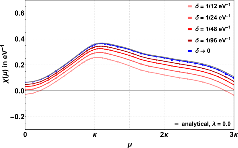
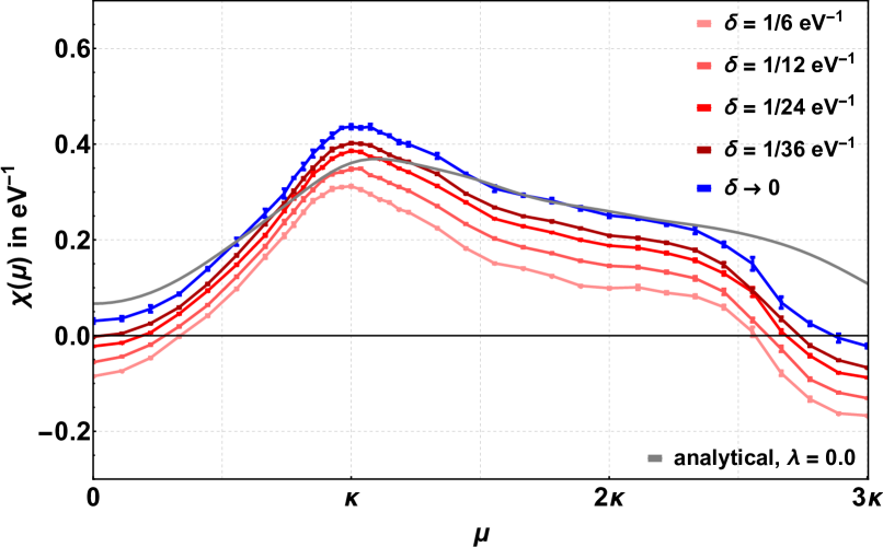
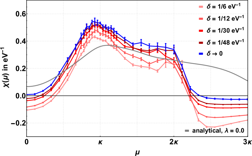
Figure 7: $\chi(\mu)$ for $\lambda=0.0$ (top), $\lambda=0.4$ (middle) and $\lambda=1.0$ (bottom) at $\beta=2\textrm{ eV}^{-1}$, $N=12$. Different discretizations are shown as well as pointwise quadratic $\delta\rightarrow 0$ extrapolations (blue). The semi-analytic $\lambda=0.0$ result obtained from Eq. (II.2) is shown for comparison in all plots (gray).

Fig. 7 (top) shows the trivial case of $\chi(\mu)$ at vanishing two-body interactions, corresponding to a Hubbard field $\phi$ which is set to zero on all lattice sites. The inversions of the fermion matrix in Eqs. (39) are straightforward to carry out in this case and no molecular dynamics trajectories are in fact needed at all. Furthermore, the disconnected part of $\chi(\mu)$ vanishes exactly in this case, as the expectation value $\langle{\rm ReTr}\,(\ldots)^{2}\rangle$ factorizes. The different curves represent calculations for different values of $\delta$, on an $N=12$ lattice at $\beta=2\textrm{ eV}^{-1}$ (from Fig. 4 we know that finite-size effects can be neglected for this choice), together with a point-by-point $\delta\to 0$ extrapolation using quadratic polynomials. As we expect, the extrapolated points agree well with the semi-analytic calculation from Eq. (II.2), with small deviations only arising from the uncertainty associated with the fitting procedure. We also see that the main effect of finite $\delta$ is a shift to lower and in some areas negative values. Fortunately, the shift is nearly constant over the entire range of $\mu$. A similar behaviour can be seen when interactions are switched on. Figs. 7 (middle and bottom) again show results from the $N=12$ lattice at $\beta=2\textrm{ eV}^{-1}$ (for $N_{t}$ between 12 and 96) but with non-zero interaction strengths corresponding to $\lambda=0.4$ and $\lambda=1.0$ respectively. For comparison, as a first indication of the effects of interactions, we also show the non-interacting limit in these figures. In order to illustrate the origin of the discretization errors in the interacting case, in Figs. 8 we also display $\chi_{\textrm{con}}(\mu)$ (top) and $\chi_{\textrm{dis}}(\mu)$ separately for $\lambda=1.0$. What is striking is that the disconnected part seems to depend only very weakly on $\delta$, while the connected part displays the familiar shift. This is a fortunate situation, as it is $\chi_{\textrm{dis}}$ which is expected to show the characteristic scaling indicative of a true thermodynamic phase transition.

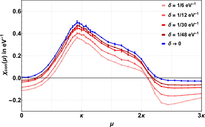
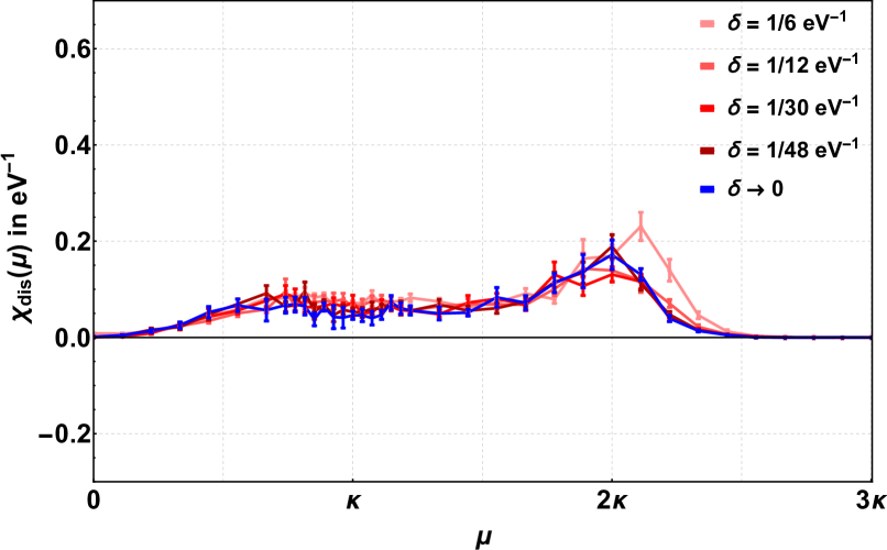
Figure 8: $\chi_{\textrm{con}}(\mu)$ (top) and $\chi_{\textrm{dis}}(\mu)$ (bottom) for $\lambda=1.0$ at $\beta=2\textrm{ eV}^{-1}$, $N=12$ for different discretizations (red) and their pointwise quadratic $\delta\rightarrow 0$ extrapolations (blue).

Our main conclusion here is that we have good justification to assume that the effect of interactions can be studied qualitatively rather well for fixed $\delta$. Nevertheless, we present a set of fully extrapolated results for $\beta=2\textrm{ eV}^{-1}$ in the following section. Results for lower temperatures will then be presented for fixed $\delta$.

IV.2 Influence of inter-electron interactions

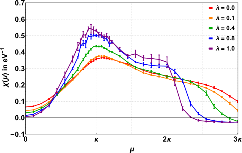
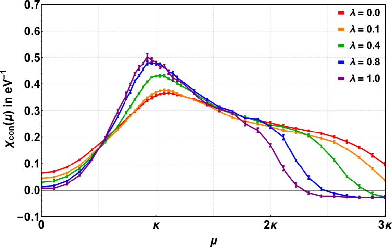
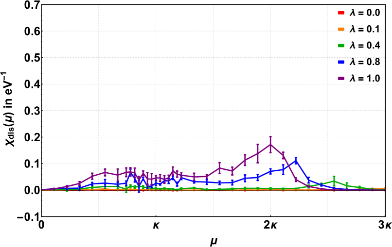
Figure 9: $\chi(\mu)$ (top), $\chi_{\textrm{con}}(\mu)$ (middle) and $\chi_{\textrm{dis}}(\mu)$ (bottom) for $\beta=2\textrm{ eV}^{-1}$, $N=12$ at different interaction strengths. All displayed points are quadratic $\delta\rightarrow 0$ extrapolations from simulations at non-zero $\delta$.

To demonstrate the effects of inter-electron interactions we have carried out the same $\delta\to 0$ extrapolations for $\beta=2\textrm{ eV}^{-1}$ , $N=12$, and $\lambda\in\left\{0.1,0.4,0.8,1.0\right\}$. As before, $\delta$ values where chosen from the set $\delta\in\left\{\frac{1}{6},\frac{1}{12},\frac{1}{18},\frac{1}{24},\frac{1}{30},\frac{1}{36},\frac{1}{48}\right\}\textrm{eV}^{-1}$ (corresponding to $N_{t}$’s between $12$ and $96$), and second order polynomials were used in all cases (the full set of $\delta$ values was only used for the cases $\lambda=0.8/1.0$). In Figs. 9 we have collected the extrapolated results for the various interaction strengths, showing the full susceptibility (top), the connected (middle) and disconnected (bottom) parts respectively. We observe that with increasing interaction strength the peak of the full susceptibility at the VHS becomes more and more pronounced. This is due to both, a corresponding rise in the connected part at the VHS and an additional contribution from the disconnected part (which is clearly non-zero for the interacting system). The peak position as well as the upper end of the conduction band are shifted towards smaller values of $\mu$. Note that we cannot disentangle the squeezing of the $\pi$-bandwidth from interactions and doping here. The combined effect certainly increases with increasing interaction strength which is qualitatively in line with experimental observations Ulstrup:2016ha . Additionally, we observe that the thermodynamically interesting disconnected part $\chi_{\textrm{dis}}$ of the susceptibility develops a second peak close to the upper end of the band (corresponding to the $\Gamma$ point) which is thus a purely interaction-driven effect.

From Figs. 9 (top and middle) it also appears that the connected part $\chi_{\textrm{con}}(\mu)$ is slightly negative at large values of $\mu$. This is clearly unphysical. We attribute it to a residual systematic error associated with the $\delta\to 0$ continuum extrapolations. We have checked that with quadratic polynomial fits the negative offset shrinks as additional points with smaller $\delta$ are included.

IV.3 Influence of temperature

This section focuses on the effect of electronic temperature (as no phonons are included, the temperature of the lattice atoms is zero by definition). All results presented in the present section were obtained for $\lambda=1$. Figs. 10 show results for $\chi(\mu)$ (top), $\chi_{\textrm{con}}(\mu)$ (middle) and $\chi_{\textrm{dis}}(\mu)$ (bottom) respectively over the entire range of the conduction bands for different temperatures. Proper lattice sizes for each temperature were chosen such that finite size effects play no role (we first estimated the necessary lattice sizes from Fig. 4, and subsequently verified the stability of the results under further increase of $N$ for individual points). All results were obtained with $\delta=1/6~{}\textrm{eV}^{-1}$, which leads to a rather large negative shift of the entire curves. Nevertheless, a clear signal can be seen for an increase of $\chi(\mu)$, not only at the VHS, but at the upper end of the band as well. What is even more striking is that from a comparison of Figs. 10 (middle and bottom) it is clear that these increases are driven mainly by the disconnected parts here, which are once more unaffected by negative offsets from the Euclidean time discretization as observed in Sec. IV.1 already.

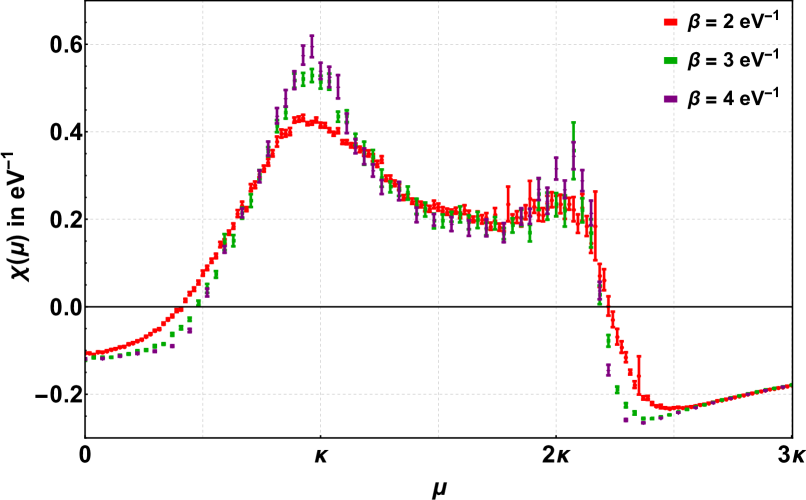
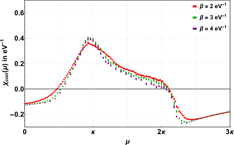
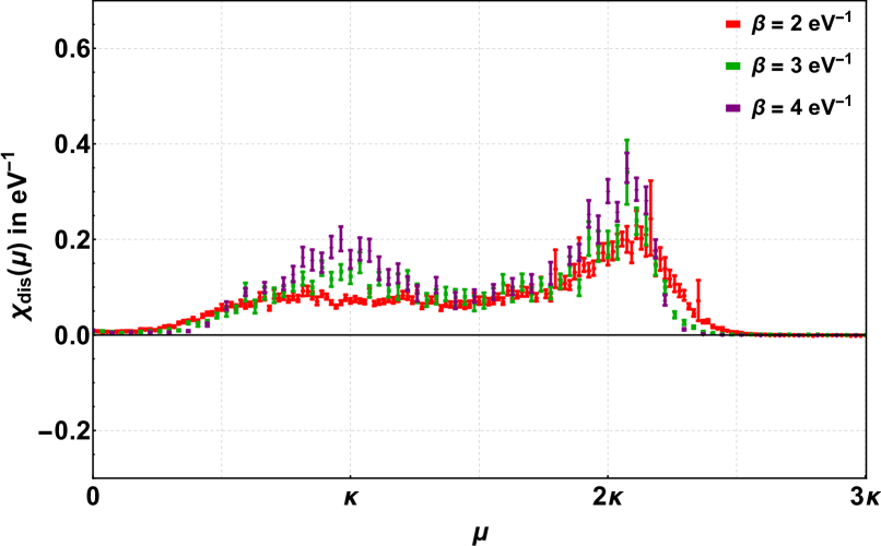
Figure 10: Temperature dependence of $\chi(\mu)$ (top), $\chi_{\textrm{con}}(\mu)$ (middle) and $\chi_{\textrm{dis}}(\mu)$ (bottom). Lattice sizes scale linearly with $\beta$, such that the displayed curves correspond to $N=12,18,24$ respectively; with $\delta=1/6~{}\textrm{eV}^{-1}$ and $\lambda=1$ for all cases.

To detect deviations from the temperature driven logarithmic divergence characteristic of the neck-disrupting Lifshitz transition and described by Eq. (11), we simulate lattices with $\delta=1/6~{}\textrm{eV}^{-1}$ in the range $\beta=1.0\ldots 6\textrm{ eV}^{-1}$ in steps of $\Delta\beta=0.5\textrm{ eV}^{-1}$. For these simulations we focused on the immediate vicinity of the VHS (the position of which does not depend strongly on temperature), generating several points in a small interval around it and using parabolic fits to identify the peak-positions and heights of $\chi/\chi_{\textrm{con}}/\chi_{\textrm{dis}}$. Obtaining a proper infinite-size limit becomes increasingly problematic for lower temperatures. In particular for $\beta=5.0\textrm{ eV}^{-1}$ and larger this turned out to be too expensive to carry out in a brute-force way. Based on the observation that the approach $N\to\infty$ depends on the lattice parity, i.e. whether its linear extend $N$ is even or odd, see Fig. 4 and the discussion thereof, we have thus devised a method to improve convergence: Since even lattices overestimate the infinite-size limit of $\chi_{\textrm{max}}$ and odd lattices underestimate it, we may expect faster convergence for average values of two subsequent lattices of different parity. We have verified that this is indeed so with $\beta=4.0\textrm{ eV}^{-1}$ and $4.5\textrm{ eV}^{-1}$, for which we compare the average values from the $N=12$ and $13$ lattices with the converged large $N$ results in Fig. 11. We then apply this averaging method for $\beta=5.0\textrm{ eV}^{-1}$, $5.5\textrm{ eV}^{-1}$ and $6\textrm{ eV}^{-1}$ where we have no brute-force results in the infinite-size limit. We expect this method to break down close to a true thermodynamic phase transition, as the usual finite-size scaling relations would then apply, but for the $\beta$ values up to $5.5\textrm{ eV}^{-1}$ successive average values from $N=11,12$ and $11,12$ lattices still have converged with good accuracy.

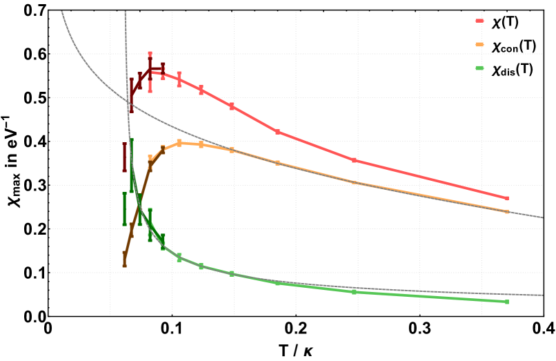
Figure 11: Temperature dependence of $\chi_{\textrm{max}}$ in the range $\beta=1.0,\ldots 6.0\textrm{ eV}^{-1}$. The lighter dots are from single lattices in the infinite volume limit, the darker dots of matching colors are obtained from average values of subsequent even and odd lattices. The dotted lines are fits using Eq. (42) for $\chi_{\textrm{con}}^{\textrm{max}}$ and Eq. (43) for $\chi_{\textrm{dis}}^{\textrm{max}}$ in appropriate ranges (see text).

Fig. 11 shows the temperature dependence of the resulting infinite-size estimates for the peak heights of $\chi/\chi_{\textrm{con}}/\chi_{\textrm{dis}}$ obtained in this way. We have identified a range of $\beta=1/T$ between $1.0$ eV^-1 and $3.0$ eV^-1 as the one over which a fit of the form

$$f_{1}(T)=a\ln\left(\frac{\kappa}{T}\right)+b+c\,\frac{T}{\kappa}$$ (41)

to the full susceptibility is possible (it breaks down if one attempts to include lower temperatures). More interestingly, however, the same fit to the connected part of the susceptibility alone is consistent with $a=3/(\pi^{2}\kappa)$ for $\beta\leq 2.5$ eV^-1 as predicted for the Lifshitz transition in the non-interacting system from Eq. (11), despite the fact that we have simulated at full interaction strength $\lambda=1$ here. A two-parameter fit to the form

$$\kappa\,\chi_{\textrm{con}}^{\textrm{max}}=\frac{3}{\pi^{2}}\ln\left(\frac{\kappa}{T}\right)+b+c\,\frac{T}{\kappa}$$ (42)

is included in Fig. 11, yielding $b=0.519(3)$ and, for the leading ${\cal O}(T)$ corrections in Eq. (11), $c=-0.472(8)$ (a three-parameter fit to the form in Eq. (41) produces $\kappa a=0.307(32)$, i.e. a central value in $1\%$ agreement with $\kappa a\!=\!3/\pi^{2}$). The result for $b$ is furthermore quite close (within 13%) to the constant in Eq. (11) as well, with a discrepancy that is within the expected offset from the discretization $\delta=1/6$ eV^-1 here. We may conclude that for the larger temperatures, where the logarithmic scaling of the peak height is observed, the behavior of the connected susceptibility basically fully agrees with that of the non-interacting tight-binding model in Eq. (11).

At temperatures below $T\sim 0.15\,\kappa$ this contribution from the electronic Lifshitz transition, which we have successfully isolated in $\chi_{\textrm{con}}$, suddenly drops in the interacting theory, however. This is contrasted by a rapid increase of the peak height of the disconnected susceptibility $\chi_{\textrm{dis}}$ here, which vanishes in the non-interacting limit. While $\chi_{\textrm{dis}}$ is negligible at high temperatures, it becomes the dominant contribution to the susceptibility at $T\sim 0.07\,\kappa$. In fact, we find that for $\beta\geq 2.5\textrm{ eV}^{-1}$ (corresponding to $T\leq 0.15\,\kappa$), $\chi_{\textrm{dis}}^{\textrm{max}}$ is well described by the model

$$f_{2}(T)=k\left|\frac{T-T_{c}}{T_{c}}\right|^{-\gamma}~{},$$ (43)

resulting in the following fit parameters:

$\beta_{c}~{}[\textrm{eV}^{-1}]$	$T_{c}~{}[\kappa]$	$\gamma~{}$	$k~{}[\textrm{eV}^{-1}]$
6.1(5)	$0.060(5)$	$0.52(6)$	$0.12(1)$

The emerging peak in $\chi^{\textrm{max}}_{\textrm{dis}}(T)$ around $\beta\approx 6$ eV^-1 is thus consistent with a powerlaw divergence indicative of a thermodynamic phase transition at non-zero $T_{c}$. Despite our efforts to produce reliable estimates for the infinite-size limits, we must expect, however, that there are still residual finite-size effects in the points closest to $T_{c}$, especially in the case of a continuous transition with a diverging correlation length. Nevertheless, the case for a powerlaw divergence at a finite temperature seems rather compelling here. All attempts to model $\chi_{\textrm{dis}}^{\textrm{max}}(T)$ using a logarithmic increase as in Eq. (41) were certainly unsuccessful, so that our conclusion seems qualitatively robust and significant.

The two most important observations are: (a) we observe good evidence of a finite transition temperature $T_{c}>0$ from the behavior of the disconnected susceptibility as an indication of the proximity to a thermodynamic phase transition as temperatures approach this $T_{c}\approx 0.06\,\kappa$ from above. (b) While the scaling exponent $\gamma\approx 0.5$ might also be interpreted as an indication of a reshaping of the saddle points in the single-particle band structure by the inter-electron interactions according to Eq. (12) with an exponent $\alpha\approx 4$ as discussed in Sec. II.1, because of the non-zero $T_{c}$ it does not have this simple description in terms of independent quasi-particles with modified single-particle energies, however. Rather, it resembles critical behavior in the vicinity of a second-order phase transition. This is in line with our observation that here it arises in the disconnected susceptibility as mentioned above.

IV.4 Antiferromagnetic spin-density wave susceptibility

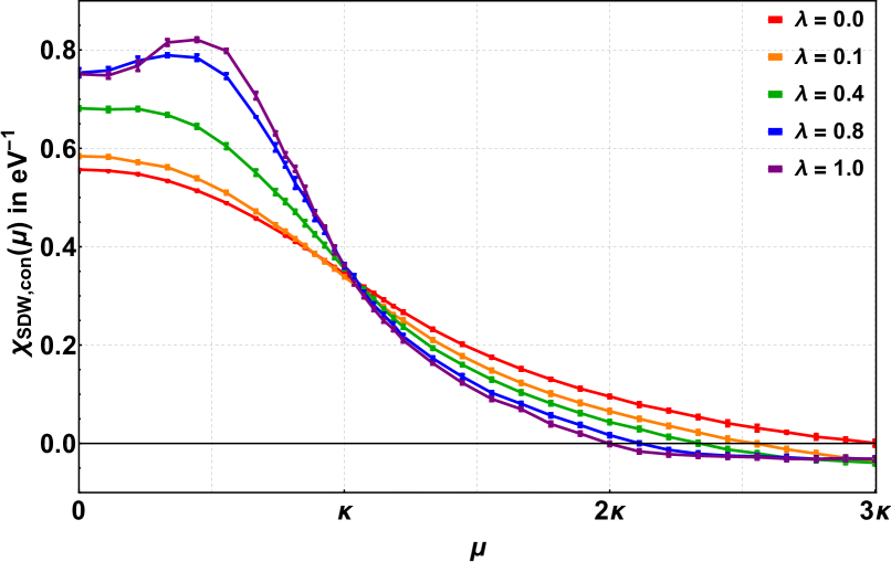
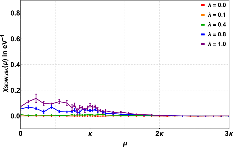
Figure 12: $\chi^{\textrm{sdw}}_{\textrm{con}}(\mu)$ (top) and $\chi^{\textrm{sdw}}_{\textrm{dis}}(\mu)$ (bottom) for $\beta=2\textrm{ eV}^{-1}$, $N=12$ at different interaction strengths. All displayed points are quadratic $\delta\rightarrow 0$ extrapolations from simulations at non-zero $\delta$.

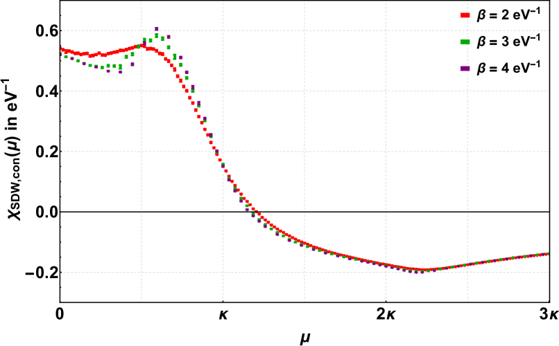
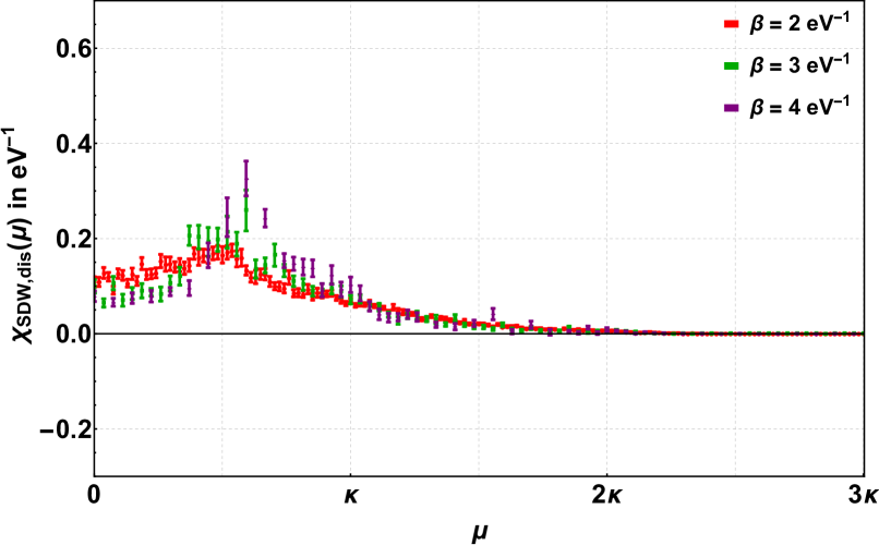
Figure 13: Temperature dependence of $\chi^{\textrm{sdw}}_{\textrm{con}}(\mu)$ (top) and $\chi^{\textrm{sdw}}_{\textrm{dis}}(\mu)$ (bottom) for $\delta=1/6~{}\textrm{eV}^{-1}$ and $\lambda=1$. Lattice sizes scale linearly with $\beta$, such that the displayed curves correspond to $N=12,18,24$ respectively.

As explained in Sec. III.1 we have used here for purely computational reasons a sublattice $s$ and spin-staggered mass $m_{s}=(-1)^{s}\,m$ in order to regulate the low-lying eigenvalues of the fermion matrix near half filling. This has the effect of introducing a small gap around the Dirac points in the single-particle energy bands by triggering an antiferromagnetic order in the ground state. For the interaction strengths $0\leq\lambda\leq 1$ considered here, this order will disappear in the limit $m\to 0$ because suspended graphene with $\lambda=1$ remains in the semimetal phase, which has been established experimentally Elias:2011 as well as in our present HMC simulation setup Ulybyshev:2013swa ; Smith:2014tha .

Nevertheless, we have also measured the corresponding susceptibility $\chi^{\textrm{sdw}}(\mu)$ for the antiferromagnetic spin-density fluctuations here. While we expect no singularity at half filling, we were particularly interested in its behavior at finite $\mu$ in our present study. With the same splitting into connected and disconnected contributions, cf. Eqs. (40), our main observations are the following: The systematics for discretization errors are completely analogous to what was discussed above (a shift of the connected part which is nearly independent of $\mu$ and almost no effect on the disconnected part). As above, in Figs. 12 we again first show the continuum extrapolated results at high temperature $\beta=2$ eV^-1 where this is still affordable. We observe an increase of $\chi^{\textrm{sdw}}(\mu=0)$ at half filling with increasing interaction strength as expected. However, in addition to this, a peak appears to form at finite $\mu$ for the larger values of $\lambda$, mainly in $\chi^{\textrm{sdw}}_{\textrm{con}}$ but to some extend also visible in $\chi^{\textrm{sdw}}_{\textrm{dis}}$ which again vanishes in the non-interacting system of course.

This peak occurs about half way between $\mu=0$ and the VHS in the vicinity of $\mu=\kappa$. When the temperature is lowered, however, it it appears to move towards the VHS while getting more and more pronounced. This is demonstrated with the ensembles at finite discretization $\delta=1/6$ eV^-1 but lower temperatures and maximal interaction strength $\lambda=1$ in Figs. 13. As before, there is no negative offset from the Euclidean-time discretization in the disconnected susceptibility which shows the increasingly sharp peak structure at the lower temperatures particularly well. Whether the peaks observed in the disconnected susceptibilities of ferromagnetic and antiferromagnetic spin-density fluctuations eventually merge and perhaps reflect the same thermodynamic phase transition when approaching $T_{c}$ certainly deserves to be further studied in the future.

V Summary and Conclusions

We have set out to study the effects of inter-electron interactions on the electronic Lifshitz transition in graphene. This neck-disrupting Lifshitz transition occurs when the Fermi-level traverses the van Hove singularity at the M-points in the bandstructure of graphene. To elucidate the effects of interactions we have first discussed in detail how the Lifshitz transition is reflected in the particle-hole susceptibility of the non-interacting system, where it is due to a logarithmic singularity of the density of states. In particular we have demonstrated how this singularity translates into a logarithmic growth of the susceptibility maximum, when viewed as a function of the chemical potential, with decreasing temperature and increasing system size.

The detailed analytical knowledge of the behavior of the particle-hole susceptibility in the non-interacting system, where it agrees with the ferromagnetic spin susceptibility, allowed us to isolate the same Lifshitz behavior also in presence of strong inter-electron interactions where it would otherwise have swamped any signs of thermodynamic singularities indicative of true phase transitions.

To search for such signs we have simulated the $\pi$-band electrons in monolayer with partially screened Coulomb interactions, combining realistic short-distance couplings with long-range Coulomb tails, using Hybrid-Monte-Carlo. This requires a chemical potential with a spin-dependent sign to circumvent the fermion-sign problem, however. We were therefore led to compare the ferromagnetic spin susceptibility with that of the non-interacting system. Despite this modification our results qualitatively resemble some of the experimental results at finite charge-carrier density. An increase of its peak-height due to interactions is in-line with the existence of an extended van Hove singularity (EVHS) as observed in ARPES experiments Bostwick:2010as . Likewise, we observe band structure renormalization (narrowing of the widths of the $\pi$-bands) due to interactions and doping Ulstrup:2016ha here as well. A possibly interesting new feature of our results is a second peak in the spin susceptibility $\chi(\mu)$ which arises near the upper end of the band. Whether this is due to some form of condensation of quasi-particle pairs near the $\Gamma$-points, which might happen because the Fermi levels of the different spin-components were shifted in opposite directions, remains to be further studied.

The electronic Lifshitz transition itself is reflected in the connected part of the susceptibility $\chi_{\textrm{con}}(\mu)$ which diverges logarithmically in the $T\to 0$ limit when $\mu$ is at the van Hove singularity. In the non-interacting system, $\chi(\mu)=\chi_{\textrm{con}}(\mu)$ and $\chi_{\textrm{dis}}(\mu)=0$. With interactions, on the other hand one has $\chi(\mu)=\chi_{\textrm{con}}(\mu)+\chi_{\textrm{dis}}(\mu)$. Interestingly, however, for higher temperatures where $\chi_{\textrm{dis}}(\mu)$ is comparatively small, the behavior of $\chi_{\textrm{con}}(\mu)$ remains precisely the same as in the non-interacting case. The electronic Lifshitz transition is entirely encoded in $\chi_{\textrm{con}}(\mu)$. Upon its subtraction from the full susceptibility one is left with $\chi_{\textrm{dis}}(\mu)$ which is moreover expected to be the relevant part in search for a thermodynamic singularity reflecting a phase transition.

In fact, our simulations provide evidence of such a thermodynamic singularity, our results are consistent with a power-law divergence of $\chi_{\textrm{dis}}$ at an electron temperature of about $T_{c}\approx 0.16\textrm{ eV}\approx 0.06\,\kappa$, which suggests that the Lifshitz transition is replaced in the interacting theory by a true quantum phase transition below $T_{c}$, and hence for $T\to 0$ with $\mu$ as the control parameter. Without identifying and isolating the Lifshitz behavior in $\chi_{\textrm{con}}(\mu)$ it would not have been possible to observe this with our present computational resources (we have already invested several hundreds of thousands of GPU hours in this project). The thermodynamic singularity is basically not visible in our present data for the full susceptibility although it will eventually dominate, sufficiently close to $T_{c}$, of course.

There are a number of possible directions for future work on the VHS. The most straightforward albeit expensive extension would be an analysis of the critical scaling close to $T_{c}$. Furthermore, of direct practical interest would be a comparison of susceptibilities associated with different types of ordered phases such as that of the antiferromagnetic spin-density wave order parameter studied as a first example at the end of the last section, or superconducting phases (e.g. chiral superconductivity Chubukov:2012as ). It should in principle be possible to identify the dominant instability of the VHS and a corresponding pairing channel.

Since the relevance of electron-phonon couplings at the VHS was demonstrated experimentally McChesney:2007uh , a quantitatively exact result should only be expected when phonons are accounted for. Furthermore, as was demonstrated e.g. in Ref. PhysRevB.86.020507 , deviations from exact Fermi-surface nesting have a profound impact on the competition between ordered phases. This implies that for a realistic description the inclusion of higher order hoppings, which suffer from a fermion-sign problem, will be necessary. For this reason, and due to the obvious fact that finite spin and charge-carrier densities have different ground states, there is a solid motivation for efforts towards dealing with the sign problem. As the Hubbard field introduced in this work has a much simpler structure than a non-Abelian gauge theory, it is conceivable that some of the more recent developments Langfeld:2014nta ; Huffman:2013mla ; Mukherjee:2014hsa ; Alexandru:2016ejd mentioned in Sec. III.2 will turn out to be useful in this context.

References

- (1) P. R. Wallace, Phys. Rev. 71 (1947), 622–634.
- (2) V. P. Gusynin, S. G. Sharapov and J. P. Carbotte, Int. J. Mod. Phys. B 21, 4611 (2007) [arXiv:0706.3016].
- (3) I. Lifshitz, Sov. Phys. JETP 11, 1130 (1960).
- (4) L. van Hove, Phys. Rev. 89, 1189 (1953).
- (5) B. Dietz, F. Iachello, M. Miski-Oglu, N. Pietralla, A. Richter, L. von Smekal, and J. Wambach, Phys. Rev. B 88, 104101 (2013) [arXiv:1304.4764].
- (6) B. Dietz, T. Klaus, M. Miski-Oglu, A. Richter, M. Wunderle, and C. Bouazza, Phys. Rev. Lett. 116, 023901 (2016) [arXiv:1512.05069].
- (7) B. Dietz, T. Klaus, M. Miski-Oglu, A. Richter, M. Bischoff, L. von Smekal and J. Wambach, Phys. Rev. Lett. 115, 026801 (2015) [arXiv:1503.04077].
- (8) W. Kohn and J. M. Luttinger, Phys. Rev. Lett., 15, 524 (1965).
- (9) R. S. Markiewicz, J. Phys. Chem. Solids, 58, 8, 1179 (1997).
- (10) J. L. McChesney, A. Bostwick, T. Ohta, T. Seyller, K. Horn, J. González and E. Rotenberg, Phys. Rev. Lett., 104, 136803 (2010).
- (11) W.S. Wang, Y.Y. Xiang, Q.H. Wang, F. Wang, F. Yang, and D.H. Lee, Phys. Rev. B. 85, 035414 (2012) [arXiv:1109.3884].
- (12) J. González, Phys. Rev. B 78, 205431 ̵͑(2008͒).
- (13) R. Nandkishore, L. S. Levitov, A. V. Chubukov, Nature Physics 8, 158–163 (2012).
- (14) M. L. Kiesel, C. Platt, W. Hanke, D. A. Abanin and R. Thomale, Phys. Rev. B, 86, 020507 (2012).
- (15) M. Yu. Kagan, V. V. Val’kov, V. A. Mitskan and M .M. Korovushkin, Solid State Communications, 188, 61-66 (2014).
- (16) A. M. Black-Schaffer and C. Honerkamp, J. Phys.: Condens. Matter 26, 423201 (2014).
- (17) T. Löthman and A. M. Black-Schaffer, Phys. Rev. B 90, 224504 (2014).
- (18) J. González, Phys. Rev. B 88, 125434 (2013).
- (19) D. Makogon, R. van Gelderen, R. Rold ̵́an and C. M. Smith, Phys. Rev. B, 84, 125404 (2011).
- (20) B. Valenzuela and M. A. H. Vozmediano, New J. Phys. 10, 113009 (2008).
- (21) C. A. Lamas, D. C. Cabra and N. Grandi, Phys. Rev. B 80, 075108 (2009).
- (22) J. P. L. Faye, M. N. Diarra and D. Sénéchal, Phys. Rev. B, 93, 155149 (2016).
- (23) M. Cranney, F. Vonau, P. B. Pillai, E. Denys, D. Aubel, M. M. D. Souza, C. Bena, and L. Simon, Europhys. Lett. 91, 66004 (2010).
- (24) J. L. McChesney, A. Bostwick, T. Ohta, K. V. Emtsev, T. Seyller, K. Horn, E. Rotenberg, arXiv:0705.3264.
- (25) K. S. Novoselov et al., Nature 438, 197 (2005) [arXiv:cond-mat/0509330].
- (26) Y. Zhang, Y. W. Tan, H. L. Stormer and P. Kim, Nature 438, 201 (2005).
- (27) D. K. Efetov, K. Philip, Phys. Rev. Lett. 105, 256805 (2010).
- (28) G. Li, A. Luican, J. M. B. Lopes dos Santos, A. H. Castro Neto, A. Reina, J. Kong and E. Y. Andrei, Nature Physics 6, 109 - 113 (2010).
- (29) A. Bostwick, T. Ohta, J. L. McChesney, T. Seyller, K. Horn and E. Rotenber, Solid State Communications, 143, 63-71 (2007).
- (30) V. Yu. Irkin, A. A. Katanin, and M. I. Katsnelson Phys. Rev. Lett. 89, 076401 (2002) [arXiv:cond-mat/0110516].
- (31) S. Ulstrup, M. Schüler, M. Bianchi, F. Fromm, C. Raidel, T. Seyller, T. Wehling and P. Hofmann, Phys. Rev. B, 94, 081403 (2016).
- (32) I. L. Aleiner, D. E. Kharzeev and A. M. Tsvelik, Phys. Rev. B 76, 195415 (2007) [arXiv:0708.0394].
- (33) T. O. Wehling et al., Phys. Rev. Lett. 106, 236805 (2011) [arXiv:1101.4007].
- (34) T. Stauber, Phys. Rev. B 82, 201404(R) (2010).
- (35) J. P. Hobson and W. A. Nierenberg, Phys. Rev. 89, 662 (1953).
- (36) A. H. Castro Neto et al., Rev. Mod. Phys. 81, 109 (2009).
- (37) Y. .M. Blanter, A. V. Pantsulaya and A. A. Varlamov, Phys. Rept. 245, 159 (1994).
- (38) R. Brower, C. Rebbi and D. Schaich, PoS LATTICE 2011, 056 (2012) [arXiv:1204.5424].
- (39) R. Brower, C. Rebbi and D. Schaich, arXiv:1101.5131.
- (40) J. E. Drut and T. A. Lähde, Phys. Rev. Lett. 102, 026802 (2009) [arXiv:0807.0834].
- (41) J. E. Drut and T. A. Lähde, Phys. Rev. B 79, 165425 (2009) [arXiv:0901.0584].
- (42) J. E. Drut and T. A. Lähde, Phys. Rev. B 79, 241405 (2009) [arXiv:0905.1320].
- (43) J. E. Drut, T. A. Lähde, and L. Suoranta, arXiv:1002.1273.
- (44) J. E. Drut and T. A. Lähde, PoS LATTICE 2011, 074 (2011) [arXiv:1111.0929].
- (45) S. Hands and C. Strouthos, Phys. Rev. B 78, 165423 (2008) [arXiv:0806.4877].
- (46) W. Armour, S. Hands and C. Strouthos, Phys. Rev. B 81, 125105 (2010) [arXiv:0910.5646].
- (47) W. Armour, S. Hands, and C. Strouthos, Phys. Rev. B 84 , 075123 (2011), [arXiv:1105.1043].
- (48) P. V. Buividovich, E. V. Luschevskaya, O. V. Pavlovsky, M. I. Polikarpov and M. V. Ulybyshev, Phys. Rev. B 86, 045107 (2012) [arXiv:1204.0921].
- (49) J. Giedt, A. Skinner, and S. Nayak, Phys. Rev. B 83, 045420 (2011) [arXiv:0911.4316].
- (50) P. V. Buividovich and M. I. Polikarpov, Phys. Rev. B 86, 245117 (2012) [arXiv:1206.0619].
- (51) M. V. Ulybyshev, P. V. Buividovich, M. I. Katsnelson and M. I. Polikarpov, Phys. Rev. Lett. 111, 056801 (2013) [arXiv:1304.3660].
- (52) D. Smith and L. von Smekal, PoS LATTICE 2013, 048 (2013) [arXiv:1311.1130].
- (53) D. Smith and L. von Smekal, Phys. Rev. B 89, 195429 (2014) [arXiv:1403.3620].
- (54) D. Smith, M. Körner and L. von Smekal, PoS LATTICE 2014, 055 (2014) [arXiv:1410.7601].
- (55) P. Buividovich, D. Smith, M. Ulybyshev and L. von Smekal, PoS LATTICE 2016, 244 (2016) [arXiv:1610.09855].
- (56) D. L. Boyda, V. V. Braguta, M. I. Katsnelson and M. V. Ulybyshev, Phys. Rev. B 94, 8, 085421 (2016) [arXiv:1601.05315].
- (57) M. V. Ulybyshev and M. I. Katsnelson, Phys. Rev. Lett. 114, 24, 246801 (2015) [arXiv:1502.01184].
- (58) P. Buividovich, D. Smith, M. Ulybyshev and L. von Smekal, arXiv:1703.05743.
- (59) T. Luu and T. A. Lähde, Phys. Rev. B 93, 15, 155106 (2016) [arXiv:1511.04918].
- (60) H.K. Tang, E. Laksono, J.N.B. Rodrigues, P. Sengupta, F.F. Assaad, S. Adam, Phys. Rev. Lett. 115, 186602 (2015).
- (61) S. Raghu, X.-L. Qi, C. Honerkamp, and Shou-Cheng Zhang Phys. Rev. Lett. 100, 156401 (2008).
- (62) S. Duane, A. D. Kennedy, B. J. Pendleton and D. Roweth, Phys. Lett. B 195, 216 (1987).
- (63) K. Langfeld, B. Lucini and A. Rago, Phys. Rev. Lett. 109, 111601 (2012) [arXiv:1204.3243].
- (64) K. Langfeld and B. Lucini, Phys. Rev. D 90, 094502 (2014) [arXiv:1404.7187].
- (65) N. Garron and K. Langfeld, Eur. Phys. J. C 76, no. 10, 569 (2016) [arXiv:1605.02709].
- (66) S. Chandrasekharan and U. J. Wiese, Phys. Rev. Lett. 83, 3116 (1999) [arXiv:cond-mat/9902128].
- (67) E. F. Huffman and S. Chandrasekharan, Phys. Rev. B 89, 111101 (2014) [arXiv:1311.0034].
- (68) Z.-X. Li, Y.-F. Jiang and H. Yao, Phys. Rev. B 91, 241117(R) (2015).
- (69) Z. C. Wei, C. Wu, Y. Li, S. Zhang, and T. Xiang Phys. Rev. Lett. 116, 250601 (2016).
- (70) Z.-X. Li, Y.-F. Jiang and H. Yao, Phys. Rev. Lett. 117, 267002 (2016).
- (71) N. Prokof’ev and B. Svistunov, Phys. Rev. Lett. 87, 160601 (2001).
- (72) Y. Delgado Mercado, C. Gattringer and A. Schmidt, Phys. Rev. Lett. 111, 141601 (2013) [arXiv:1307.6120].
- (73) A. Mukherjee and M. Cristoforetti, Phys. Rev. B 90, 035134 (2014) [arXiv:1403.5680].
- (74) A. Alexandru, G. Basar, P. F. Bedaque, G. W. Ridgway and N. C. Warrington, Phys. Rev. D 95, 014502 (2017) [arXiv:1609.01730].
- (75) D. Sexty, PoS LATTICE 2014, 016 (2014) [arXiv:1410.8813].
- (76) T. Boz, P. Giudice, S. Hands, J. I. Skullerud and A. G. Williams, AIP Conf. Proc. 1701, 060019 (2016) [arXiv:1502.01219].
- (77) L. Holicki, J. Wilhelm, D. Smith, B. Wellegehausen and L. von Smekal, LATTICE 2016, 052 (2017) [arXiv:1701.04664].
- (78) A. Maas, L. von Smekal, B. Wellegehausen and A. Wipf, Phys. Rev. D 86, 111901 (2012) [arXiv:1203.5653].
- (79) B. H. Wellegehausen and L. von Smekal, PoS LATTICE 2014, 177 (2015) [arXiv:1501.06706].
- (80) W. Detmold, K. Orginos and Z. Shi, Phys. Rev. D 86, 054507 (2012) [arXiv:1205.4224].
- (81) B. B. Brandt and G. Endrodi, PoS LATTICE 2016, 039 (2016) [arXiv:1611.06758].
- (82) D. C. Elias et al., Nature Physics 7, 701 - 704 (2011).