Introduction to Flavour Physics and $CP$ Violation

Abstract

These lecture notes provide an introduction to the theoretical concepts of flavour physics and $CP$ violation, based on a series of lectures given at the ESHEP 2016 summer school. In the first lecture we review the basics of flavour and $CP$ violation in the Standard Model. The second lecture is dedicated to the phenomenology of $K$ and $B$ meson decays, where we focus on a few representative observables. In the third lecture we give an introduction to flavour physics beyond the Standard Model, both within the framework of Minimal Flavour Violation and beyond.

Introduction

Flavour physics and $CP$ violation have played a central role in the development of the Standard Model (SM). It was the underlying $SU(3)$ flavour symmetry of mesons and baryons that lead Gell-Mann to the introduction of up, down, and strange quarks as the fundamental constituents of hadronic matter [GellMann:1964nj]. The charm quark was predicted prior to its discovery as an explanation for the smallness of the $K_{L}\to\mu^{+}\mu^{-}$ decay rate [Glashow:1970gm]. It was then realized that, in order to account for the observed $CP$ violation in neutral kaon mixing, a third generation of quarks was needed [Kobayashi:1973fv]. Furthermore, the heaviness of the top quark was predicted from the size of $CP$ violation in $K^{0}-\bar{K}^{0}$ mixing and of the neutral $B$ meson oscillations prior to its discovery [Buras:1993wr].

Subsequently, the role of flavour physics has shifted from the discovery of the building blocks of the SM to the measurement of its parameters. The majority of the SM parameters is related to the flavour sector and can thus be determined in flavour violating decays. With increasing experimental and theoretical accuracy, their determination has by now reached an impressive precision.

Having at hand a good understanding of the SM flavour sector, the measurement of flavour and $CP$-violating processes can be used to put constraints on models of New Physics (NP). Due to the strong suppression of flavour violation in the SM, very high energy scales can be probed in this way, well beyond the reach of direct searches for new particles in high energy collisions at the Large Hadron Collider (LHC) (see [Buras:2013ooa] for a recent review). NP around the TeV scale is therefore required to have a highly non-trivial flavour structure.

The present lecture notes provide a summary of a series of three lectures given at the European School for High Energy Physics (ESHEP) 2016 in Skeikampen, Norway. The topic of these lectures is restricted to quark flavour physics. Flavour in the charged lepton and neutrino sector has been covered by Gabriela Barenboim [Barenboim:2016ili]. In lecture 0.1 we introduce the quark Yukawa couplings and the Cabibbo-Kobayashi-Maskawa (CKM) matrix as the basic ingredients of flavour and $CP$ violation in the SM. We then discuss the physics of flavour changing neutral currents and review their description in terms of an effective Hamiltonian and the path from quark level flavour transitions to the decays of mesons. Lecture 0.2 is devoted to the phenomenology of flavour and $CP$-violating decays of kaons and $B$ mesons. Rather than providing an exhaustive overview, we focus on a number of particularly interesting benchmark processes, like neutral meson mixings, rare $K$ meson decays, and the recently observed anomalies in $B$ meson decays based on semileptonic $b\to s$ transitions. In lecture 0.3 we turn our attention to flavour physics beyond the SM. After reviewing the generic constraints on the scale of NP from flavour and $CP$-violating decays, we discuss two well-known suppression mechanisms for the size of new flavour violating interactions. We motivate the concept of Minimal Flavour Violation (MFV) from the flavour symmetries of the SM. As an alternative to MFV, we also discuss how models with partially composite fermions can explain the observed flavour hierarchies in the SM, and at the same time suppress flavour changing neutral currents to an acceptable level.

A large number of excellent lecture notes on the physics of flavour and $CP$ violation can be found on the arXiv. As a few representative examples, let me recommend especially the lectures by Gino Isidori [Isidori:2013ez], Yuval Grossmann [Grossman:2010gw], and Andrzej j. Buras [Buras:2005xt]. An extensive pedagogical introduction into the technicalities of the theory of flavour physics can be found in [Buras:1998raa].

0.1 Flavour Physics in the Standard Model

0.1.1 Quark Yukawa Couplings and the CKM Matrix

In nature, all fundamental matter fields – quarks, charged leptons, and neutrinos – come in three copies, the so-called flavours. They can be collected in three fermion generations, with increasing masses, but otherwise identical quantum numbers. The subject of flavour physics is the description of interactions between the various flavours, with the goal to unravel the underlying dynamics of flavour symmetry breaking.

In the SM, the left-handed quarks are arranged in doublets of the $SU(2)_{L}$ weak interactions:

$$Q_{j}=\pmatrix{u}_{L}\\ d_{L},\pmatrix{c}_{L}\\ s_{L},\pmatrix{t}_{L}\\ b_{L}\,,$$ (1)

while the right-handed quarks are introduced as $SU(2)_{L}$ singlets:

$$U_{j}=u_{R},c_{R},t_{R}\qquad D_{j}=d_{R},s_{R},b_{R}\,.$$ (2)

The quarks’ couplings to the gluons, weak gauge bosons $W^{\pm}$ and $Z$, and the photon are described by the kinetic term in the Lagrangian

$$\mathcal{L}_{\text}{fermion}=\sum_{j=1}^{3}\bar{Q}_{j}i\slashed D_{Q}Q_{j}+\bar{U}_{j}i\slashed D_{U}U_{j}+\bar{D}_{J}i\slashed D_{D}D_{j}\vspace{-3mm}\,,$$ (3)

with the covariant derivatives

$$D_{Q,\mu} = \partial_{\mu}+ig_{s}T^{a}G^{a}_{\mu}+ig\tau^{a}W^{a}_{\mu}+ig^{\prime}Q^{Y}_{Q}B_{\mu}\,,$$ (4)

$$D_{U,\mu} = \partial_{\mu}+ig_{s}T^{a}G^{a}_{\mu}\hskip 51.21504pt+ig^{\prime}Q^{Y}_{U}B_{\mu}\,,$$ (5)

$$D_{D,\mu} = \partial_{\mu}+ig_{s}T^{a}G^{a}_{\mu}\hskip 51.21504pt+ig^{\prime}Q^{Y}_{D}B_{\mu}\,,$$ (6)

and the hypercharges assigned as $Q^{Y}_{Q}=1/6$, $Q^{Y}_{U}=2/3$, $Q^{Y}_{D}=-1/3$. $T^{a}(a=1,\dots,8)$ and $\tau^{a}(a=1,2,3)$ are the generators of $SU(3)_{c}$ and $SU(2)_{L}$, respectively, and the index $j$ runs over the three generations of quark fields. It is evident that the gauge couplings are universal for all three generations.

Flavour non-universality, on the other hand, is introduced by the quark Yukawa couplings to the Higgs field, responsible for the generation of non-zero quark masses:

$$\mathcal{L}_{\text}{Yuk}=\sum_{i,j=1}^{3}(-Y_{U,ij}\bar{Q}_{Li}\tilde{H}U_{Rj}-Y_{D,ij}\bar{Q}_{Li}HD_{Rj}+h.c.)\,,$$ (7)

where $h.c.$ abbreviates the hermitian conjugate term. The subscripts $i,j$ are generation indices, and the dual field $\tilde{H}$ is given as $\tilde{H}=\epsilon H^{*}=(H^{0*},-H^{-})^{T}$. Replacing the Higgs field $H$ by its vacuum expectation value $\langle H\rangle=(0,v)^{T}$, we obtain the quark mass terms

$$\sum_{i,j=1}^{3}(-m_{U,ij}\bar{u}_{Li}u_{Rj}-m_{D,ij}\bar{d}_{Li}d_{Rj}+h.c.)\,,$$ (8)

with the quark mass matrices given by $m_{U,D}=vY_{U,D}$.

The quark mass matrices $m_{U}$ amd $m_{D}$ are $3\times 3$ complex matrices in flavour space with a priori arbitrary entries. They can be diagonalized by making appropriate bi-unitary field redefinitions:

$$u_{L}=\hat{U}_{L}u_{L}^{m}\,,\qquad u_{R}=\hat{U}_{R}u_{R}^{m}\,,\qquad d_{L}=\hat{D}_{L}d_{L}^{m}\,,\qquad d_{R}=\hat{D}_{R}d_{R}^{m}\,,$$ (9)

with the superscript ^m denoting quarks in their mass eigenstate basis.

Is the SM Lagrangian invariant under these transformations? Unitary transformations of the right-handed quark sector are indeed unphysical, as they drop out from the rest of the Lagrangian. However, $u_{Li}$ and $d_{Li}$ form the $SU(2)_{L}$ doublets $Q_{i}$ (with $i=1,2,3$). Their kinetic term gives rise to the interaction

$$\frac{g}{\sqrt{2}}\bar{u}_{Li}\gamma_{\mu}W^{\mu+}d_{Li}\,.$$ (10)

Transformation of eq:Wint to the mass eigenstate basis yields

$$\frac{g}{\sqrt{2}}\bar{u}_{Li}\hat{U}_{L,ij}^{\dagger}\hat{D}_{L,jk}\gamma_{\mu}W^{\mu+}d_{Lk}\,.$$ (11)

We conclude that the combination

$$\hat{V}_{\text}{CKM}=\hat{U}_{L}^{\dagger}\hat{D}_{L}$$ (12)

is physical, it is called the CKM matrix [Cabibbo:1963yz, Kobayashi:1973fv]. It describes the misalignment between left-handed up- and down-type quark mass eigenstates, which leads to flavour violating charged current interactions, mediated by the $W^{\pm}$ bosons. It is convenient to label the elements of $\hat{V}_{\text}{CKM}$ by the quark flavours involved in the respective charged current interaction:

$$\hat{V}_{\text}{CKM}=\pmatrix{V}_{ud}&V_{us}V_{ub}\\ V_{cd}V_{cs}V_{cb}\\ V_{td}V_{ts}V_{tb}\,.$$ (13)

For example, the element $V_{ub}$ appears in the coupling of a bottom and an up quark to the $W$ boson.

0.1.2 Standard Parametrization of the CKM Matrix

Let us now determine the number of physical parameters in the CKM matrix. Being a unitary $3\times 3$ matrix, it can be parametrized by three mixing angles and six complex phases in general. However, five of these phases are unphysical, as they can be absorbed as unobservable parameters into the up-type and down-type quarks, respectively. Note that an overall phase rotation of all quarks does not affect the CKM matrix. We are then left with three mixing angles $\theta_{12}$, $\theta_{23}$, $\theta_{13}$ and one complex phase $\delta$ as the physical parameters of the CKM matrix. Introducing the short-hand notation $s_{ij}=\sin\theta_{ij}$ and $c_{ij}=\cos\theta_{ij}$, the standard parametrization of the CKM matrix reads [Chau:1984fp]

$$\hat{V}_{\text}{CKM}=\pmatrix{c}_{12}c_{13}&s_{12}c_{13}s_{13}e^{-i\delta}\\ -s_{12}c_{23}-c_{12}s_{23}s_{13}e^{i\delta}c_{12}c_{23}-s_{12}s_{23}s_{13}e^{i\delta}s_{23}c_{13}\\ s_{12}s_{23}-c_{12}c_{23}s_{13}e^{i\delta}-c_{12}s_{23}-s_{12}c_{23}s_{13}e^{i\delta}c_{23}c_{13}\,.$$ (14)

Note that this parametrization is recommended by the Particle Data Group (PDG) [Olive:2016xmw].

Alternatively, the number of independent flavour parameters in the SM can also be determined from symmetry principles. Ignoring the Yukawa couplings, the SM quark sector has a global

$$G_{\text}{flavour}=U(3)_{Q}\times U(3)_{U}\times U(3)_{D}$$ (15)

flavour symmetry. The quark Yukawa couplings $Y_{U}$, $Y_{D}$ explicitly break $G_{\text}{flavour}$, leaving only a single $U(1)$ factor unbroken, that corresponds to the overall phase of the quark fields. This $U(1)$ symmetry is associated to baryon number conservation, which is an accidental symmetry of the SM. We can use this symmetry breaking pattern to count the number of flavour parameters.

We start from the Yukawa couplings $Y_{U}$ and $Y_{D}$. A priori, these are arbitrary complex $3\times 3$ matrices, hence they bring in nine real parameters and nine complex phases each. However, not all of these $18+18$ parameters are physical. In fact, each of the broken generators of the flavour symmetry group $G_{\text}{flavour}$ corresponds to an unphysical parameter in the Lagrangian which can be removed by making appropriate field redefinitions. A $3\times 3$ unitary matrix contains three real parameters and six complex phases. The three $U(3)$ factors in $G_{\text}{flavour}$ therefore carry nine real parameters and 18 phases. All but one of them, namely the phase corresponding to the unbroken overall $U(1)$, correspond to unphysical parameters that can be removed from $Y_{U}$ and $Y_{D}$. We are then left with a total of nine real parameters in the quark flavour sector and one physical complex phase. The nine real parameters are the quark masses $m_{u},m_{d},m_{c},m_{s},m_{t},m_{b}$ and the three mixing angles $\theta_{12},\theta_{13},\theta_{23}$ of the CKM matrix, and the phase is simply the CKM phase $\delta$.

Experimentally, it has been found that the CKM matrix exhibits a rather strong hierarchy, with [Olive:2016xmw]

$$s_{12}\sim 0.2\,,\qquad s_{23}\sim 0.04\,,\qquad s_{13}\sim 4\cdot 10^{-3}\,.$$ (16)

The CKM matrix hence is close to the unit matrix, with hierarchical off-diagonal elements. Flavour changing transitions are therefore strongly suppressed in the SM. Similarly, also the quark masses are found to follow a hierarchical pattern, spanning five orders of magnitude in size. The lack of a more fundamental theory explaining the origin of this structure is referred to as the flavour hierarchy problem of the SM.

0.1.3 $CP$ violation in the SM

We have seen above that the angles $\theta_{ij}$ of the CKM matrix parametrize the amount of flavour mixing between the quarks of the generations $i$ and $j$. The amount of flavour violation in the SM is therefore quantified by the values of the CKM mixing angles. But what is the physical meaning of the presence of a complex phase $\delta$?

In order to understand this, let us consider two discrete transformations:

• the parity transformation

  $$P:\psi(r,t)\to\gamma^{0}\psi(-r,t)$$ (17)

  which transforms left-handed fermion fields into right-handed ones and vice versa, and

• the charge conjugation

  $$C:\psi\to i(\bar{\psi}\gamma^{0}\gamma^{2})^{T}$$ (18)

  which transforms left(right)-handed quarks into left(right)-handed antiquarks.

It is evident from equations eq:Lfermion–eq:DDmu that the weak interactions violate both $C$ and $P$, as they treat left- and right-handed quarks differently.

But what about the combination of both transformations, $CP$? A $CP$ transformation connects left-handed quarks to right-handed antiquarks. It is easy to convince oneself that the neutral current interactions mediated by gluons, the photon and the $Z$ boson are indeed invariant under $CP$. Let us then look at the charged current interactions mediated by the $W^{\pm}$ bosons:

$$\mathcal{L}_{c.c.} = \frac{g}{\sqrt{2}}V_{ik}\bar{u}_{Li}\gamma_{\mu}W^{\mu+}d_{Lk}+h.c.$$ (19)

$$= \frac{g}{\sqrt{2}}V_{ik}\bar{u}_{Li}\gamma_{\mu}W^{\mu+}d_{Lk}+\frac{g}{\sqrt{2}}V_{ik}^{*}\bar{d}_{Lk}\gamma_{\mu}W^{\mu-}u_{Li}$$

$$\xrightarrow{CP} \frac{g}{\sqrt{2}}V_{ik}\bar{d}_{Lk}\gamma_{\mu}W^{\mu-}u_{Li}+\frac{g}{\sqrt{2}}V_{ik}^{*}\bar{u}_{Li}\gamma_{\mu}W^{\mu+}d_{Lk}$$

$$= \frac{g}{\sqrt{2}}V_{ik}^{*}\bar{u}_{Li}\gamma_{\mu}W^{\mu+}d_{Lk}+h.c.$$

We see that $CP$ conjugation replaces the CKM element $V_{ik}$ by its complex conjugate. Hence, the $CP$ symmetry is violated in the SM by the presence of a non-vanishing complex phase $\delta\neq 0$ in the CKM matrix.

It is important to note, however, that the phase $\delta$ is not a physical parameter, as, by means of the aforementioned rephasing of quark fields, it can be shifted to different elements of the CKM matrix. A parametrization-independent and therefore physical measure of $CP$ violation is instead given by the Jarlskog invariant [Jarlskog:1985ht, Jarlskog:1985cw]

$$J_{CP}=\text{Im}(V_{us}V_{cb}V_{ub}^{*}V_{cs}^{*})\,.$$ (20)

Experimentally, the Jarlskog invariant is found to be $J_{CP}\simeq 3\cdot 10^{-5}$.

0.1.4 Flavour Changing Neutral Currents

We have seen above that flavour changing charged currents are present at the tree level in the SM, with the size of the interactions governed by the off-diagonal elements of the CKM matrix. Flavour changing neutral currents (FCNCs), on the other hand, are absent at the tree level in the SM. In order to see this, let us have a closer look at the $Z$ boson coupling to left-handed down-type quarks, as an illustrative example. Transforming the coupling of the quark flavour eigenstates $d_{Lj}$ into a coupling of the quark mass eigenstates $d_{Li}^{m}$, we find

$$\mathcal{L}_{\text}{n.c} \ni g_{Z}(d_{L})\,\bar{d}_{Lj}\gamma_{\mu}Z^{\mu}d_{Lj}$$ (21)

$$= g_{Z}(d_{L})\,\bar{d}_{Li}^{m}(\hat{D}_{L}^{\dagger})_{ij}\gamma_{\mu}Z^{\mu}(\hat{D}_{L})_{jk}d_{Lk}^{m}$$

$$= g_{Z}(d_{L})\,\bar{d}_{Li}^{m}\gamma_{\mu}Z^{\mu}\delta_{ik}d_{Lk}^{m}\,,$$

where

$$g_{Z}(d_{L})=\frac{g}{\cos\theta_{W}}\left(-\frac{1}{2}+\frac{1}{3}\sin^{2}\theta_{W}\right)$$ (22)

is the $Z$ boson coupling to left-handed down-type quarks. We can see that due to the unitarity of the flavour rotation matrix $\hat{D}_{L}$, the coupling remains flavour diagonal and flavour universal. The same argument holds for all neutral gauge boson couplings in the SM.

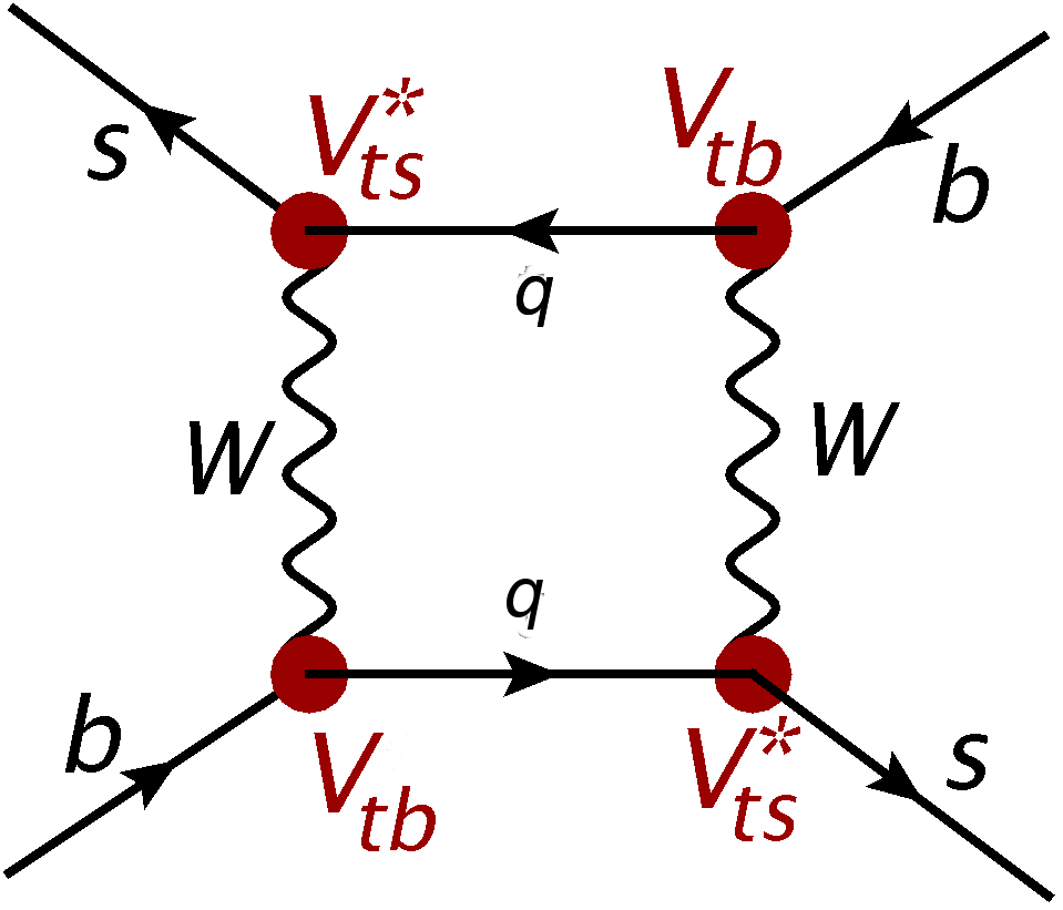
Figure 1: One loop diagram for $B_{s}-\bar{B}_{s}$ mixing in the SM.

FCNCs are however generated in the SM by loop diagrams with internal $W^{\pm}$ bosons. As an example, figure 1 shows the one loop diagram that generates the leading contribution to neutral $B_{s}$ meson mixing. The mixing amplitude generated by this contribution is schematically given by

$$\mathcal{M}\propto\sum_{i,j=u,c,t}V_{is}^{*}V_{ib}V_{js}^{*}V_{jb}F(x_{i},x_{j})\,.$$ (23)

Here, $F(x_{i},x_{j})$ is the relevant one loop function, with $x_{i}=(m_{i}/M_{W})^{2}$, and the double sum runs over the internal quark flavours. Using the CKM unitarity

$$\sum_{i=u,c,t}V_{is}^{*}V_{ib}=0\,,$$ (24)

setting $m_{u}=0$ and neglecting contributions proportional to $V_{cs}^{*}V_{cb}\ll V_{ts}^{*}V_{tb}$, this can be simplified to

$$\mathcal{M}\propto(V_{ts}^{*}V_{tb})^{2}S_{0}(x_{t})\,,$$ (25)

with

$$S_{0}(x_{t})=F(x_{t},x_{t})-2F(0,x_{t})+F(0,0)\,.$$ (26)

We can see that, indeed, FCNCs are generated by loop processes in the SM. However they are suppressed not only by the smallness of the off-diagonal CKM elements, but also by the so-called GIM mechanism [Glashow:1970gm]: All contributions that are independent of the masses of the quarks running in the loop are cancelled by the unitarity of the CKM matrix, and only the differences of mass-dependent terms survive. While above we have seen the GIM mechanism at work for one loop contributions, it in fact holds to all orders.

0.1.5 The Unitarity Triangle

The hierarchical structure of the CKM matrix can be used to derive an alternative parametrization, which turns out to be very useful for estimating the size of flavour violating transitions. In the Wolfenstein parametrization [Wolfenstein:1983yz]

$$\hat{V}_{\text}{CKM}=\pmatrix{1}-\frac{\lambda^{2}}{2}&\lambda A\lambda^{3}(\rho-i\eta)\\ -\lambda 1-\frac{\lambda^{2}}{2}A\lambda^{2}\\ A\lambda^{3}(1-\rho-i\eta)-A\lambda^{2}1+\mathcal{O}(\lambda^{4})\,,$$ (27)

$\lambda=|V_{us}|\sim 0.2$ is the only small parameter, while $A$, $\rho$, and $\eta$ are $\mathcal{O}(1)$. It is therefore convenient to estimate the size of flavour violating decays by making an expansion in powers of $\lambda$. The accuracy of this expansion can be improved by changing the parameters of the Wolfenstein parametrization to [Buras:1994ec, Schmidtler:1991tv]

$$\lambda\,,\qquad A\,,\qquad\bar{\rho}=\left(1-\frac{\lambda^{2}}{2}\right)\rho\,,\qquad\bar{\eta}=\left(1-\frac{\lambda^{2}}{2}\right)\eta\,.$$ (28)

As discussed before, the CKM matrix is a unitary matrix, and not all of its elements are independent parameters. Various relations hold among them, which can be tested experimentally. One of the most popular ones,

$$V_{ud}V_{ub}^{*}+V_{cd}V_{cb}^{*}+V_{td}V_{tb}^{*}=0\,,$$ (29)

can be displayed as a triangle in the complex plane, the so-called unitarity triangle (UT) [Jarlskog:1988ii]. With the base of the UT normalized to unity, the apex is simply given by $(\bar{\rho},\bar{\eta})$. The sides $R_{b}$ and $R_{t}$, as shown in figure 2, are given by

$$R_{b} = \left|\frac{V_{ud}V_{ub}^{*}}{V_{cd}V_{cb}^{*}}\right|=\left(1-\frac{\lambda^{2}}{2}\right)\frac{1}{\lambda}\frac{|V_{ub}|}{|V_{cb}|}\,,$$ (30)

$$R_{t} = \left|\frac{V_{td}V_{tb}^{*}}{V_{cd}V_{cb}^{*}}\right|=\frac{1}{\lambda}\frac{|V_{td}|}{|V_{cb}|}\,.$$ (31)

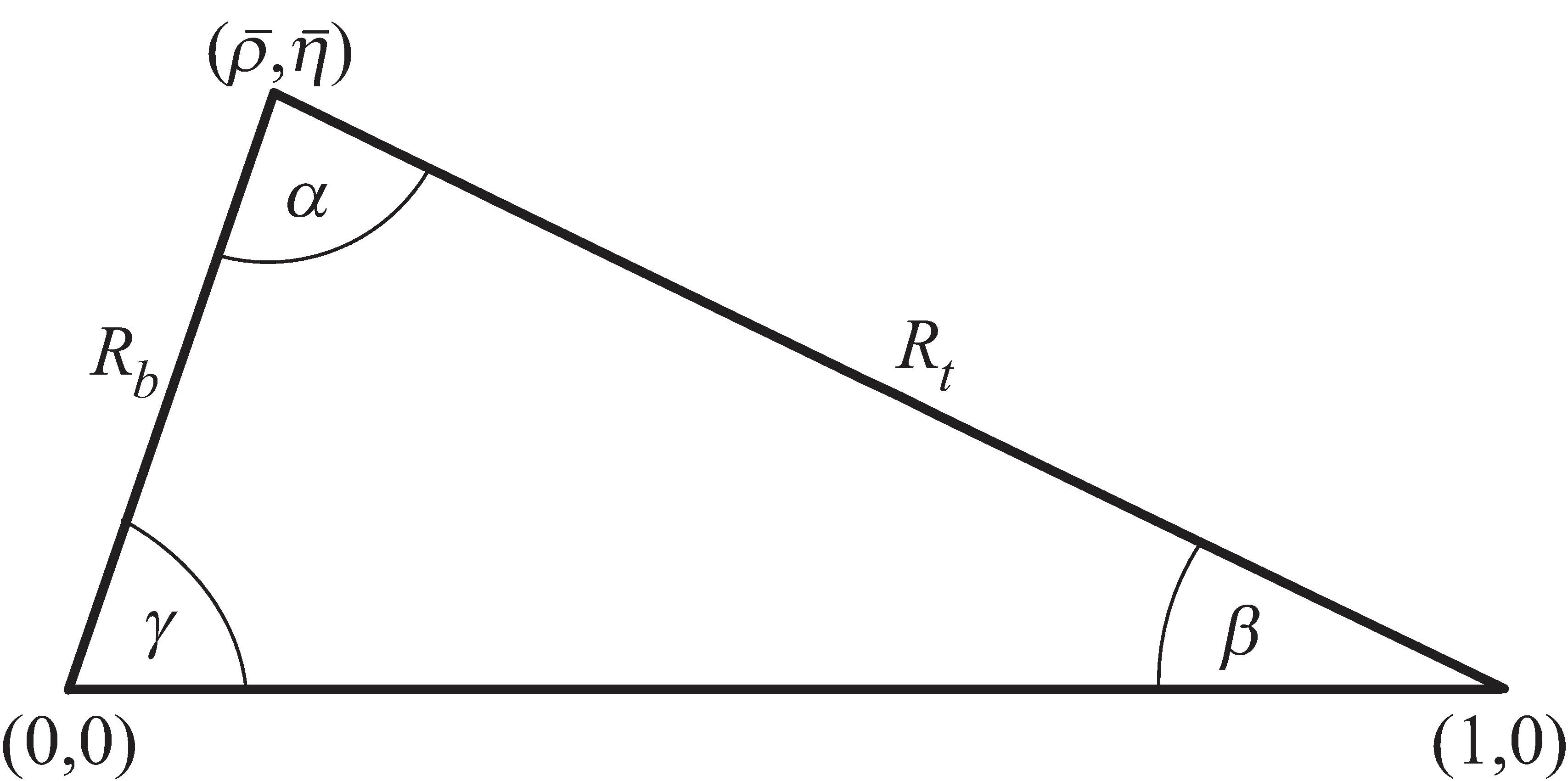
Figure 2: Unitarity triangle.

For the UT angles, two notations are commonly used in the literature. They are related to each other as follows:

$$\alpha\equiv\phi_{2}\,,\qquad\beta\equiv\phi_{1}\,,\qquad\gamma\equiv\phi_{3}\,.$$ (32)

The UT can be determined experimentally from various measurements of flavour violating decays of $K$ and $B$ mesons. A special role in this determination is played by the length of the side $R_{b}$ and the angle $\gamma$: Being sensitive to the absolute values and $CP$-violating phases of the elements $V_{ub}$ and $V_{cb}$, they can be determined from $B$ decays governed by tree level charged current interactions. It is therefore a good approximation to assume that NP contributions to these measurements are negligible. The measurement of $|V_{ub}|$, $|V_{cb}|$ and $\gamma=\arg(-V_{ud}V_{ub}^{*}/V_{cd}V_{cb}^{*})$ then leaves us with the reference unitarity triangle [Grossman:1997dd], which determines the CKM matrix independently of potential NP contributions to rare flavour violating decays.

The length of the side $R_{t}$ and the angle $\beta$, on the other hand, depend on CKM elements involving the top quark. Hence, they can only be measured in loop-induced flavour changing neutral current (FCNC) processes. Due to their strong suppression in the SM, these observables are sensitive to NP contributions. A model-independent determination of the CKM matrix using these quantities is therefore not possible. NP contributions to the loop induced processes used in the determination of the UT

The strategy to hunt for NP contributions to flavour violating observables is then as follows. First, the CKM matrix and the UT have to be determined from tree level charged current decays as accurately as possible. As this determination is independent of potential NP contributions, the result can be used as input for precise SM predictions of rare, loop-induced FCNC processes. These predictions are then to be compared with the data, which – in case of a discrepancy – would yield an unambiguous sign of a NP contribution to the decay in question. Clearly, in order to be able to claim a NP discovery in flavour violating observables, a solid understanding of the SM contribution and its uncertainties is mandatory.

0.1.6 The effective Hamiltonian

An important theoretical complication arises in the study of quark flavour violating decays. Due to the confinement of QCD at low energies, quarks do not appear as free particles in nature, but are bound in hadrons. Therefore, not only the weak interactions leading to flavour violation, as discussed above, have to be well understood, but also the strong dynamics describing the bound states of QCD. The latter interactions, taking place at the typical hadronic energy scales of a few hundred MeV to a few GeV, are non-perturbative and hence, with our current methods, cannot be calculated analytically.

A convenient theoretical tool to handle these various contributions from processes ar different energy scales is provided by the operator product expansion [Wilson:1969zs]. In this framework, effective flavour violating operators are obtained from integrating out the heavy electroweak (EW) gauge bosons $W^{\pm}$ and $Z$ and the top quark at the EW scale, and then connecting these operators with the low energy QCD interactions responsible for hadronic interactions. The latter are comprised in matrix elements of the effective operators, involving the initial and final state mesons of the decay in question. These matrix elements, being governed by non-perturbative interactions, cannot be calculated analytically, but have to evaluated using non-perturbative methods like lattice QCD or QCD sum rules (see e. g. [Lellouch:2011qw] and [Radyushkin:1998du] for pedagogical introductions) , unless it is possible to extract them from the data.

To summarize, in order to arrive at a theoretical description of flavour violating meson decays, the following five steps have to be taken:

1. Calculation of the weak interaction process governing the underlying flavour violating quark decay.

2. Construction of the low energy effective Hamiltonian by integrating out the heavy degrees of freedom (i. e. $W^{\pm}$, $Z$, $t$).

3. Renormalization group running from the scale $\mu\sim M_{W}$ of weak interactions to the hadronic scale $\mu\sim\text{GeV}$.

4. Collection of non-perturbative effects in QCD matrix elements involving initial and final state mesons.

5. Evaluation of matrix elements using non-perturbative methods (lattice QCD, QCD sum rules etc.) or extraction from data.

To better understand how this is done in practice, let us have a look at two simple examples. First we consider the semileptonic charged current decay $B\to\pi\ell\nu$ from which the CKM element $|V_{ub}|$ can be obtained. Then we sketch the SM prediction for neutral $B_{s}$ meson mixing.

Semileptonic charged currents: $B\to\pi\ell\nu$

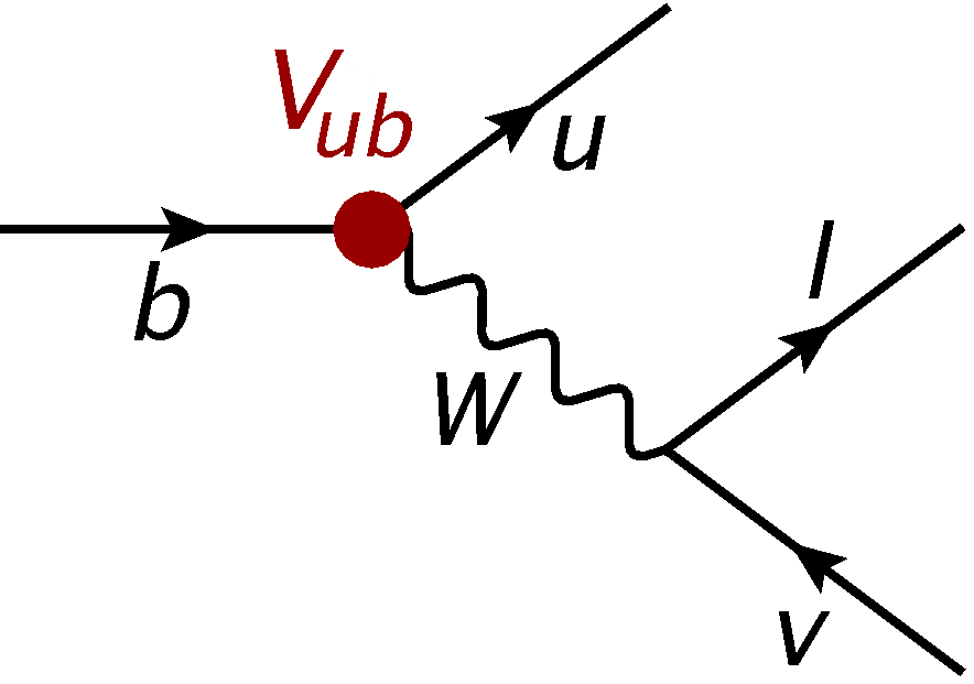
Figure 3: Tree level diagram mediating the $b\to u\ell\nu$ decay.

The element $|V_{ub}|$ can be determined from the semileptonic charged current transition $b\to u\ell\nu$, occurring at the tree level in the SM. Evaluating the relevant Feynman diagram shown in figure 3, we find

$$\mathcal{M}=\frac{g}{\sqrt{2}}V_{ub}(\bar{u}\gamma^{\mu}P_{L}b)\frac{g_{\mu\nu}}{p^{2}-M_{W}^{2}}\frac{g}{\sqrt{2}}(\bar{\ell}\gamma^{\nu}P_{L}\nu)\,.$$ (33)

Neglecting the momentum transfer $p^{2}\ll M_{W}^{2}$ in the $W$ propagator, and using the short hand notation $2(\bar{f}\gamma^{\mu}P_{L}f^{\prime})=(\bar{f}f^{\prime})_{V-A}$, $\mathcal{M}$ simplifies to

$$\mathcal{M}=-\frac{g^{2}}{2M_{W}^{2}}V_{ub}(\bar{u}b)_{V-A}(\bar{\ell}\nu)_{V-A}\,.$$ (34)

Introducing the well-known Fermi constant

$$\frac{G_{F}}{\sqrt{2}}=\frac{g^{2}}{8M_{W}^{2}}\,,$$ (35)

we obtain the tree level effective Hamiltonian

$$\mathcal{H}_{\text}{eff}=\frac{4G_{F}}{\sqrt{2}}V_{ub}(\bar{u}b)_{V-A}(\bar{\ell}\nu)_{V-A}+h.c.\,.$$ (36)

In order to obtain an accurate expression for the $B\to\pi\ell\nu$ decay, the known QCD corrections have to be taken into account, including the renormalization group running from the weak scale, where the $W$ boson is integrated out, to the $B$ meson scale. The non-perturbative QCD effects describing the $B\to\pi$ transition generated by the effective Hamiltonian $\mathcal{H}_{\text}{eff}$ are collected in the matrix element

$$\langle\pi|(\bar{b}u)_{V-A}|B\rangle\,,$$ (37)

which has been calculated by lattice QCD.

From the measurement of the $B^{0}\to\pi^{-}\ell^{+}\nu$ branching ratio, one can then extract the value [Lattice:2015tia] (see also [Dalgic:2006dt, Flynn:2015mha])

$$|V_{ub}|=(3.72\pm 0.16)\cdot 10^{-3}\,.$$ (38)

Note again that as the $B^{0}\to\pi^{-}\ell^{+}\nu$ is generated at the tree level in the SM, NP contributions are expected to be negligible. Therefore the determination of $|V_{ub}|$ in eq:Vub holds model-independently. In a similar way, also $|V_{us}|$, $|V_{cb}|$ and the UT angle $\gamma$ can be determined from tree level decays, independently of NP in flavour violating decays.

$B_{s}-\bar{B}_{s}$ mixing

As discussed in section 0.1.4, neutral $B_{s}$ meson mixing in the SM is driven by the one loop box diagram in figure 1. We have seen that due to the GIM mechanism and the hierarchical structure of the CKM matrix, only the mass-dependent part of the top quark contribution is relevant. Including a factor $\eta_{B}=0.55\pm 0.01$ [Buras:1990fn, Urban:1997gw] that comprises perturbative QCD corrections and the renormalization group evolution down to the $B$ meson scale, the effective Hamiltonian can be written as

$$\mathcal{H}_{\text}{eff}=\frac{G_{F}^{2}}{16\pi^{2}}M_{W}^{2}\eta_{B}(V_{tb}^{*}V_{ts})^{2}S_{0}(x_{t})(\bar{b}s)_{V-A}(\bar{b}s)_{V-A}+h.c.\,,$$ (39)

with the one loop function $S_{0}(x_{t})$ given by

$$S_{0}(x_{t})=\frac{4x_{t}-11x_{t}^{2}+x_{t}^{3}}{4(1-x_{t})^{2}}-\frac{3x_{t}^{3}\ln x_{t}}{2(1-x_{t})^{3}}\,.$$ (40)

Sandwiching $\mathcal{H}_{\text}{eff}$ between the initial and final state mesons, we obtain the mixing matrix element

$$M_{12}=\frac{1}{2m_{B_{s}}}\left\langle\bar{B}_{s}\left|\mathcal{H}_{\text}{eff}\right|B_{s}\right\rangle^{*}\,.$$ (41)

Again, the hadronic matrix element $\left\langle\bar{B}_{s}\left|(\bar{b}s)_{V-A}(\bar{b}s)_{V-A}\right|B_{s}\right\rangle$ comprises the low-energy QCD dynamics of the mesonic process. It has been calculated by lattice QCD with an impressive precision.

Using the CKM matrix determined from tree level decays, the SM predictions for $B_{s}-\bar{B}_{s}$ mixing observables, like the mass difference $\Delta M_{s}$ and the $CP$-violating phase $\phi_{s}$ can then be compared with the data. This comparison yields a good agreement of the measured values with their SM predictions, leaving only little room for NP contributions. In lecture 0.3 we will have a closer look at the constraints on NP models from flavour violating observables.

0.2 Phenomenology of $K$ and $B$ Meson Decays

0.2.1 Theory of Neutral Kaon Mixing

In the first lecture, we have briefly sketched the theoretical description of $B_{s}-\bar{B}_{s}$ mixing in the SM, paying particular attention to specific details like the GIM mechanism and the construction of the effective Hamiltonian. In this section, we aim at a more thorough derivation of neutral meson mixing. While we focus on the case of kaon mixing in what follows, a generalization to neutral $B$ and $D$ mesons is straightforward.

Two neutral pseudoscalar $K$ mesons exist, the $|K^{0}\rangle=|d\bar{s}\rangle$ and the $|\bar{K}^{0}\rangle=|s\bar{d}\rangle$. They are each other’s antiparticles and transform under $CP$ as

$$CP|K^{0}\rangle=-|\bar{K}^{0}\rangle\,,\qquad CP|\bar{K}^{0}\rangle=-|K^{0}\rangle\,.$$ (42)

As we can deduce from section 0.1.4, $K^{0}$ and $\bar{K}^{0}$ can mix by one loop box diagrams in the SM. The time evolution of the $K^{0}-\bar{K}^{0}$ system is therefore described by the two-component Schrödinger equation

$$i\frac{d\psi(t)}{dt}=\hat{H}\psi(t)\,,\qquad\psi(t)=\pmatrix{K}^{0}(t)\\ \bar{K}^{0}(t)$$ (43)

with the $2\times 2$ Hamiltonian

$$\hat{H}=\hat{M}-i\frac{\hat{\Gamma}}{2}=\pmatrix{M}_{11}&M_{12}\\ M_{21}M_{22}-\frac{i}{2}\pmatrix{\Gamma}_{11}&\Gamma_{12}\\ \Gamma_{21}\Gamma_{22}\,.$$ (44)

Here, $\hat{M}$ is the dispersive part of the Hamiltonian, and $\hat{\Gamma}$ is the absorptive part. Since both $\hat{M}$ and $\hat{\Gamma}$ are hermitian, we have

$$M_{21}=M_{12}^{*}\,,\qquad\Gamma_{21}=\Gamma_{12}^{*}\,.$$ (45)

In addition, $CPT$ invariance implies

$$M_{11}=M_{22}\equiv M\,,\qquad\Gamma_{11}=\Gamma_{22}\equiv\Gamma\,,$$ (46)

so that the Hamiltonian simplifies to

$$\hat{H}=\pmatrix{M}-\frac{i}{2}\Gamma&M_{12}-\frac{i}{2}\Gamma_{12}\\ M^{*}_{12}-\frac{i}{2}\Gamma_{12}^{*}M-\frac{i}{2}\Gamma$$ (47)

Diagonalizing $\hat{H}$, we obtain the mass eigenstates

$$K_{L,S}=\frac{(1+\bar{\varepsilon})K^{0}\pm(1-\bar{\varepsilon})\bar{K}^{0}}{\sqrt{2(1+|\bar{\varepsilon}|^{2})}}\,,$$ (48)

where $L$ and $S$ stand for ‘long’ and ‘short’, respectively, and refer to the different lifetimes of the two states. The parameter $\bar{\varepsilon}$ is defined through

$$\frac{1-\bar{\varepsilon}}{1+\varepsilon}=\sqrt{\frac{M^{*}_{12}-\frac{i}{2}\Gamma_{12}^{*}}{M_{12}-\frac{i}{2}\Gamma_{12}}}=\frac{\Delta M-\frac{i}{2}\Delta\Gamma}{2M_{12}-i\Gamma_{12}}\,.$$ (49)

Experimentally $\bar{\varepsilon}$ is found to be of the order $\mathcal{O}(10^{-3})$. Therefore the mass difference $\Delta M$ and the width difference $\Delta\Gamma$ are well approximated by the simple expressions

$$\Delta M=M_{L}-M_{S}=2\,\text{Re}M_{12}\,,\qquad\Delta\Gamma=\Gamma_{L}-\Gamma_{S}=2\,\text{Re}\Gamma_{12}\,.$$ (50)

0.2.2 $CP$ Violation in the Neutral Kaon Sector

As we have seen before, $K^{0}$ and $\bar{K}^{0}$ transform into each other under $CP$ conjugation. The CP eigenstates are therefore given by

$$K_{1}=\frac{1}{\sqrt{2}}(K^{0}-\bar{K}^{0})\,,\qquad K_{2}=\frac{1}{\sqrt{2}}(K^{0}+\bar{K}^{0})\,.$$ (51)

$K_{1}$ is even under $CP$ conjugation, while $K_{2}$ is $CP$-odd. Comparing the $CP$ eigenstates in eq:K-CP to the mass eigenstates in eq:K-mass, it becomes clear that the mass eigenstates $K_{L,S}$ are not pure $CP$ eigenstates. Instead they contain a small admixture of the state with opposite $CP$ parity:

$$K_{S}=\frac{K_{1}+\bar{\varepsilon}K_{2}}{\sqrt{1+|\bar{\varepsilon}|^{2}}}\,,\qquad K_{L}=\frac{K_{2}+\bar{\varepsilon}K_{1}}{\sqrt{1+|\bar{\varepsilon}|^{2}}}\,.$$ (52)

This mixture of states with opposite $CP$ parities implies that the $CP$ symmetry is violated in neutral kaon mixing.

The two mass eigenstates, $K_{L}$ and $K_{S}$ are found experimentally to have very different lifetimes [Olive:2016xmw]:

$$\tau(K_{S})\sim 90\,\text{ps}\,,\qquad\tau(K_{L})\sim 5\cdot 10^{3}\,\text{ps}\,.$$ (53)

The explanation can be found in the $CP$ properties of the two states: $K_{S}$ is basically the $CP$-even state $K_{1}$, with a small $CP$-odd admixture. $K_{L}$, on the other hand, is approximately the $CP$-odd state $K_{2}$, with a small $CP$-even admixture. Now if $CP$ is conserved in the decay of neutral kaons, then the $CP$-even state $K_{1}$ will decay into two pions, forming a $CP$-even final state. $K_{2}$, however, has to decay into a $CP$-odd final state, which contains three pions. As the three pion final state is phase space suppressed with respect to the two pion final state, the $K_{1}$ decay rate is much faster, so that its lifetime is much shorter than the one of $K_{2}$. The observed lifetime difference suggests that indeed $CP$ is, at least approximately, conserved and $\bar{\varepsilon}$ is small.

In 1964, the decay $K_{L}\to\pi^{+}\pi^{-}$ has been observed [Christenson:1964fg], yielding the first experimental confirmation that $CP$ symmetry is violated. In 1980, the Nobel Prize has been awarded to Cronin and Fitch for this discovery.

The mere discovery of the $K_{L}\to\pi^{+}\pi^{-}$ decay however does not tell us where the observed $CP$ violation originates from. $CP$ can either be violated in the neutral kaon mixing, if the mass eigenstates $K_{L,S}$ are not CP eigenstates. Or $CP$ can be violated in the decay – in that case the $CP$-odd state $K_{2}$ can decay into a $CP$-even two pion final state. Last but not least, in general, $CP$ can also be violated in the interference of mixing and decay amplitudes.

How can we distinguish whether $CP$ is violated in the mixing (also called indirect $CP$ violation) or in the decay process (direct $CP$ violation)? The key idea is that the amount of direct $CP$ violation depends on the decay channel, but indirect $CP$ violation does not.

Hence, to disentangle the two types of $CP$ violation, we study the following set of $K\to\pi\pi$ decay modes:

$$K_{L}\to\pi^{0}\pi^{0}\,,\qquad K_{L}\to\pi^{+}\pi^{-}\,,$$ (54)

$$K_{S}\to\pi^{0}\pi^{0}\,,\qquad K_{S}\to\pi^{+}\pi^{-}\,.$$ (55)

As the charged and neutral pions form an isospin triplet, the two pion final state can have either isospin $I=0$ or $I=2$. The decay amplitudes into charged and neutral pions can therefore be writen as

$$A(K^{0}\to\pi^{+}\pi^{-}) = \sqrt{\frac{2}{3}}A_{0}e^{i\delta_{0}}+\sqrt{\frac{1}{3}}A_{2}e^{i\delta_{2}}\,,$$ (56)

$$A(K^{0}\to\pi^{0}\pi^{0}) = \sqrt{\frac{2}{3}}A_{0}e^{i\delta_{0}}-2\sqrt{\frac{1}{3}}A_{2}e^{i\delta_{2}}\,.$$ (57)

Here, $A_{0}$ and $A_{2}$ parametrize the decay amplitudes in the $I=0$ and $I=2$ final states, respectively. The ‘strong phases’ $\delta_{0}$ and $\delta_{2}$ do not change sign under $CP$ conjugation.

Defining then the ratios

$$\eta_{00}=\frac{A(K_{L}\to\pi^{0}\pi^{0})}{A(K_{S}\to\pi^{0}\pi^{0})}\,,\qquad\eta_{+-}=\frac{A(K_{L}\to\pi^{+}\pi^{-})}{A(K_{S}\to\pi^{+}\pi^{-})}\,,$$ (58)

it is possible to disentangle $CP$ violation in neutral kaon mixing, parametrized by $\varepsilon$, from direct $CP$ violation in the $K\to\pi\pi$ decays, parametrized by $\varepsilon^{\prime}$. One can show that

$$\varepsilon\simeq\frac{1}{3}\left(\eta_{00}+2\eta_{+-}\right)\,,\qquad\text{Re}\left(\frac{\varepsilon^{\prime}}{\varepsilon}\right)\simeq\frac{1}{6}\left(1-\left|\frac{\eta_{+-}}{\eta_{00}}\right|^{2}\right)\,.$$ (59)

0.2.3 Status of $\varepsilon$ and $\varepsilon^{\prime}$

Both $|\varepsilon|$ and Re$(\varepsilon^{\prime}/\varepsilon)$ have been measured with high precision, with the results [Olive:2016xmw]

$$|\varepsilon| = (2.228\pm 0.011)\cdot 10^{-3}\,,$$ (60)

$$\text{Re}(\varepsilon^{\prime}/\varepsilon) = (16.6\pm 2.3)\cdot 10^{-4}\,.$$ (61)

In the SM, $CP$ violation in the kaon sector is strongly suppressed. As the presence of three quark generations is needed for $CP$ violation, both $\varepsilon$ and $\varepsilon^{\prime}$ are generated by top quark contributions. The effect is therefore proportional to the combination of CKM elements

$$\text{Im}(V_{ts}^{*}V_{td})\simeq\mathcal{O}(10^{-4})\,.$$ (62)

$CP$ violation in the kaon sector is thus strongly suppressed in the SM. In the presence of NP, however, this strong CKM suppression can be absent, depending on the flavour structure of the model. $CP$-violating observables in the kaon sector therefore have an outstanding sensitivity to NP contributions.

For the parameter $\varepsilon$ a simple yet precise formula can be derived:

$$\varepsilon=\frac{\kappa_{\varepsilon}e^{i\varphi_{\varepsilon}}}{\sqrt{2}\Delta M_{K}}\text{Im}M_{12}\,.$$ (63)

Here, the mass splitting $\Delta M_{K}=(0.5292\pm 0.0009)\cdot 10^{-2}\,\text{ps}^{-1}$ and the phase $\varphi_{\varepsilon}=43.51^{\circ}$ have been measured precisely [Olive:2016xmw]. The parameter $\kappa_{\varepsilon}$ comprises corrections from long-distance dynamics, and has been estimated to be $\kappa_{\varepsilon}=0.94\pm 0.02$ [Buras:2008nn, Buras:2010pza].

The off-diagonal element $M_{12}$ of the mixing amplitude is, as discussed above, generated by box diagrams in the SM. While its real part receives sizeable long-distance contributions, the $CP$-violating imaginary part is driven by short distance dynamics and therefore under good theoretical control. Including the known higher oder perturbative corrections and the non-perturbative parameter $\hat{B}_{K}$ obtained from lattice QCD calculations, one finds [Brod:2011ty]

$$|\varepsilon|_{\text}{SM}=(1.90\pm 0.26)\cdot 10^{-3}\,,$$ (64)

which is a bit lower albeit still consistent with the data.

Due to its strong suppression in the SM, $\varepsilon$ is very sensitive to potential NP contributions. The good agreement of the measured value with its SM prediction therefore results in strong constraints on the NP entering $K^{0}-\bar{K}^{0}$ mixing. We will return to this topic in more detail in the third lecture.

The ratio $\varepsilon^{\prime}/\varepsilon$ has recently received a lot of attention. While its measured value in eq:epe-exp has been available since the late 1990s, until recently no reliable SM prediction was available. The situation changed when the first lattice QCD calculations of the relevant $K\to\pi\pi$ hadronic matrix elements became available. The result reads [Bai:2015nea]

$$B_{6}^{(1/2)}=0.57\pm 0.19\,,\qquad B_{8}^{(3/2)}=0.76\pm 0.05\,.$$ (65)

While this result, in particular the one for $B_{6}^{(1/2)}$, still carries sizeable uncertainties, it is interesting to note its consistency with the bound

$$B_{6}^{(1/2)}<B_{8}^{(3/2)}<1\,,$$ (66)

that has recently been derived using large $N_{c}$ counting and the dual QCD approach [Buras:2015xba, Buras:2016fys].

The result for the hadronic matrix elements in eq:B6B8 can then be plugged into the simple phenomenological expression for $\varepsilon^{\prime}/\varepsilon$ in the SM [Buras:2003zz, Buras:2015yba]:

$$\text{Re}(\varepsilon^{\prime}/\varepsilon)_{\text}{SM}=\frac{\text{Im}(V_{ts}^{*}V_{td})}{1.4\cdot 10^{-4}}\cdot 10^{-4}\cdot\Big{(}{-3.6+21.4B_{6}^{(1/2)}}+{1.2-10.4B_{8}^{(3/2)}}\Big{)}\,,$$ (67)

which has been derived using the calculation of perturbative QCD contributions at next-to-leading order (NLO).

The first two terms in the brackets of eq:epe-phen stem from the $I=0$ amplitude which is dominantly generated by QCD penguin contributions. The last two terms, on the other hand, originate in the $I=2$ amplitude, caused mainly by EW penguin contributions. The numerical values of these contributions, together with the result for the hadronic matrix elements, leads to a large cancellation between the $I=0$ and $I=2$ contributions to $\text{Re}(\varepsilon^{\prime}/\varepsilon)_{\text}{SM}$. Due to this cancellation, a precise knowledge of the hadronic matrix elements $B_{6}^{(1/2)}$ and $B_{8}^{(3/2)}$ is of utmost importance for an accurate prediction of $\text{Re}(\varepsilon^{\prime}/\varepsilon)$ in the SM. Using the result in eq:B6B8, one finds [Buras:2015yba]

$$\text{Re}(\varepsilon^{\prime}/\varepsilon)_{\text}{SM}=(1.4\pm 4.6)\cdot 10^{-4}\,.$$ (68)

This prediction is significantly lower than the measured value in eq:epe-exp, revealing a $2.9\sigma$ tension. A consistent result has been obtained in [Kitahara:2016nld]. It is interesting to note that the central value in eq:epe-SM is much lower than the long-standing result in [Pallante:2001he], although consistent due to the large uncertainties in the latter analysis. We are looking forward to future improved lattice QCD calculations by several groups which will clarify the present situation and hopefully strengthen the indicated hint for NP.

Having at hand only a single lattice result for the hadronic matrix elements in question, it would clearly be premature to claim the presence of NP in $\varepsilon^{\prime}/\varepsilon$. The observed tension, however, is intriguing. Due to its strong suppression in the SM, the ratio $\varepsilon^{\prime}/\varepsilon$ is extremely sensitive to NP contributions. It is therefore conceivable that NP would first be observed in this observable, even if other flavour data measured so far show little or no discrepancy with their SM predictions.

Following the recent progress on the theoretical understanding of $\varepsilon^{\prime}/\varepsilon$, this observable has been revisited in the context of various NP models [Blanke:2015wba, Buras:2015yca, Buras:2015jaq, Buras:2015kwd, Buras:2016dxz, Tanimoto:2016yfy, Kitahara:2016otd, Bobeth:2016llm]. It turns out that several extensions of the SM can significantly enhance $\varepsilon^{\prime}/\varepsilon$ and thereby reconcile the theory prediction with the data. In addition, many NP scenarios predict simultaneous large deviations from the SM prediction of the rare decay $K_{L}\to\pi^{0}\nu\bar{\nu}$, with the sign of the latter effect depending on the structure of the model.

0.2.4 Rare $K$ Decays

Rare and $CP$-violating kaon decays, like the aforementioned decay $K_{L}\to\pi^{0}\nu\bar{\nu}$, offer a unique opportunity to look for NP. These decays, mediated by $s\to d$ FCNC transitions at the quark level, are strongly suppressed in the SM by the hierarchical structure of the CKM matrix and the GIM mechanism. Consequently, large NP effects are possible even if the NP mass scale is much beyond the TeV scale. Of particular interest are the decay modes $K^{+}\to\pi^{+}\nu\bar{\nu}$ and $K_{L}\to\pi^{0}\nu\bar{\nu}$, as they are not only strongly suppressed in the SM but also theoretically extremely clean. Therefore, an outstanding NP sensitivity is provided by these decays. In fact, it has been shown within a simplified model analysis that a flavour violating $Z^{\prime}$ gauge boson can lead to large effects in the $K\to\pi\nu\bar{\nu}$ decays even if its mass is in the $10^{3}$ TeV range [Buras:2014zga].

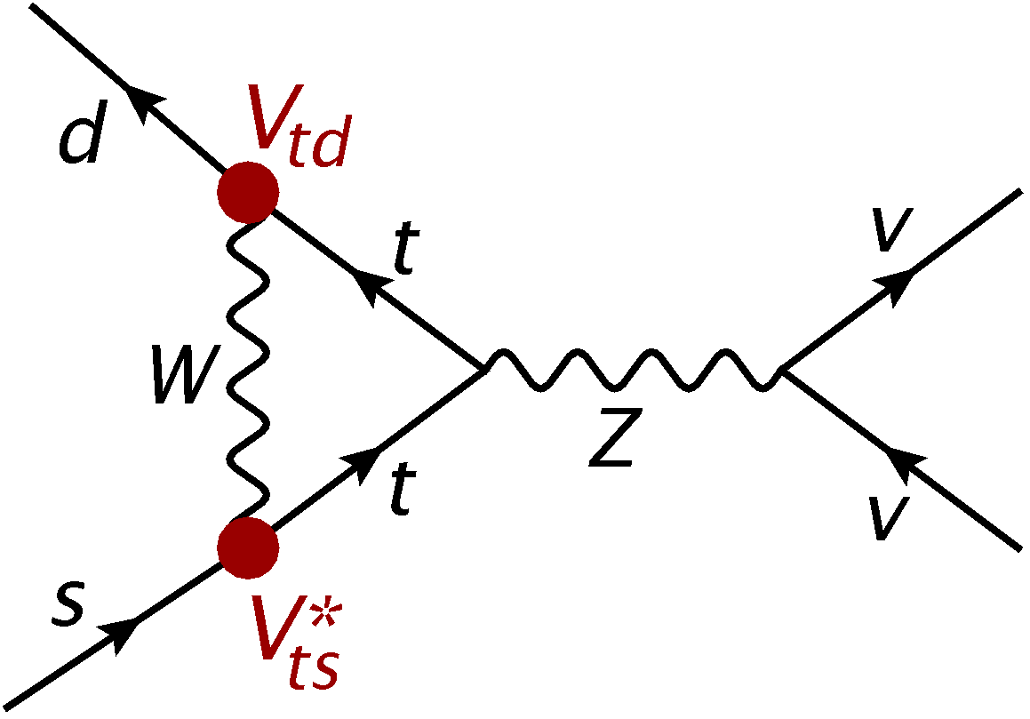
Figure 4: $Z$-penguin diagram contributing to $K\to\pi\nu\bar{\nu}$ in the SM.

In the SM, the $K\to\pi\nu\bar{\nu}$ decays are governed by $Z$-penguin and box diagrams like the ones shown in figure 4. The effective Hamiltonian reads [Buchalla:1995vs]

$$\mathcal{H}_{\text}{eff}=\frac{G_{F}}{\sqrt{2}}\frac{\alpha}{2\pi\sin^{2}\theta_{W}}\sum_{\ell=e,\mu,\tau}\left(V_{cs}^{*}V_{cd}X^{\ell}_{\text}{NNL}(x_{c})+V_{ts}^{*}V_{td}X(x_{t})\right)(\bar{s}d)_{V-A}(\bar{\nu}_{\ell}\nu_{\ell})_{V-A}\,.$$ (69)

The first term in the brackets corresponds to the charm quark contribution which is known to NNLO in QCD [Buras:2005gr, Buras:2006gb] and NLO in the EW theory [Brod:2008ss]. It is relevant only for the $CP$-conserving decay $K^{+}\to\pi^{+}\nu\bar{\nu}$. The second term stems from the top quark contribution which affects both the $CP$-conserving mode $K^{+}\to\pi^{+}\nu\bar{\nu}$ and the $CP$-violating mode $K_{L}\to\pi^{0}\nu\bar{\nu}$.

The relevant $\langle\pi|(\bar{s}d)_{V-A}|K\rangle$ matrix elements can be extracted from the data on $K^{+}\to\pi^{0}e^{+}\nu$ with high precision, making use of isospin symmetry. The main uncertainties is the SM prediction for the $K\to\pi\nu\bar{\nu}$ branching ratios therefore stem from the determination of the relevant CKM elements. Of particular importance is the value of $|V_{cb}|$ and, for $K_{L}\to\pi^{0}\nu\bar{\nu}$, the UT angle $\gamma$. The current SM prediction for the two branching ratios is [Buras:2015qea]

$$\mathcal{B}(K^{+}\to\pi^{+}\nu\bar{\nu}) = (8.4\pm 1.0)\cdot 10^{-11}\,,$$ (70)

$$\mathcal{B}(K_{L}\to\pi^{0}\nu\bar{\nu}) = (3.4\pm 0.6)\cdot 10^{-11}\,.$$ (71)

A big experimental effort to measure these decays is currently underway at the NA62 experiment [Rinella:2014wfa] at CERN and the KOTO experiment [Yamanaka:2012yma] at J-PARC in Japan.

NP contributions to $\mathcal{H}_{\text}{eff}$ in eq:Heff-kpnn can be parametrized model-independently by replacing the SM top-loop funcion $X(x_{t})$ by a general complex function [Buras:2004ub]

$$X\equiv|X|e^{i\theta_{X}}\,.$$ (72)

NP in the $K\to\pi\nu\bar{\nu}$ system can therefore be described by two independent parameters $|X|$ and $\theta_{X}$. Measuring both $\mathcal{B}(K^{+}\to\pi^{+}\nu\bar{\nu})$ and $\mathcal{B}(K_{L}\to\pi^{0}\nu\bar{\nu})$ determines both parameters, and observing

$$|X|\neq X(x_{t})\qquad\text{and/or}\qquad\theta_{X}\neq 0$$ (73)

would be an unambiguous sign of NP.

Determining both $|X|$ and $\theta_{X}$ not only provides a clean test of the SM, but in case of a non-vanishing NP contribution also allows to draw conclusions about the structure of NP contributions to neutral kaon mixing [Blanke:2009pq]. The reason is quite simple to understand. If the effective flavour changing $s\to d$ transition is, as in the SM, purely left-handed, then the same NP structure is responsible for $K^{0}-\bar{K}^{0}$ mixing and for the $K\to\pi\nu\bar{\nu}$ decays. In particular, the same $CP$-violating phase $\theta_{K}$ enters, only mutliplied by a factor of two for $K^{0}-\bar{K}^{0}$ mixing. The constraint on NP from $\Delta M_{K}$ is much weaker than the one from $\varepsilon$, so that any NP contribution to $K^{0}-\bar{K}^{0}$ mixing must be predominantly real: $2\theta_{K}\simeq 0,\pi$. The phase $\theta_{K}$ measured in the $K\to\pi\nu\bar{\nu}$ decays is then restricted to the values

$$\theta_{K}\simeq 0,\frac{\pi}{2},\pi,\frac{3\pi}{2}\,.$$ (74)

In the plane showing the branching ratios $\mathcal{B}(K^{+}\to\pi^{+}\nu\bar{\nu})$ and $\mathcal{B}(K_{L}\to\pi^{0}\nu\bar{\nu})$, these values for $\theta_{K}$ correspond to two straight lines: a horizontal one, where $\mathcal{B}(K_{L}\to\pi^{0}\nu\bar{\nu})$ remains SM-like as the NP contribution is $CP$-conserving, and a slanted one which is parallel to the model-independent Grossman-Nir bound [Grossman:1997sk]. This pattern is depicted by the green lines in figure 5. If on the other hand, both left- and right-handed FCNCs are induced by NP, then neutral kaon mixing will usually be dominated by the so-called “left-right” effective operators containing both chiralities. In that case the correlation with the $K\to\pi\nu\bar{\nu}$ decays is lost, and no correlation between $\mathcal{B}(K^{+}\to\pi^{+}\nu\bar{\nu})$ and $\mathcal{B}(K_{L}\to\pi^{0}\nu\bar{\nu})$ arises. The full range for the two branching ratios, shown in red in figure 5, is then possible.

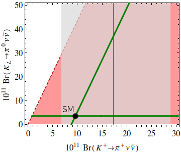
Figure 5: Model-distinguishing correlation between $\mathcal{B}(K^{+}\to\pi^{+}\nu\bar{\nu})$ and $\mathcal{B}(K_{L}\to\pi^{0}\nu\bar{\nu})$ [Blanke:2009pq].

The discussed correlation between $\mathcal{B}(K^{+}\to\pi^{+}\nu\bar{\nu})$ and $\mathcal{B}(K_{L}\to\pi^{0}\nu\bar{\nu})$ has indeed been found in a number of NP models with purely left-handed FCNC transitions [Blanke:2006eb, Buras:2012dp, Buras:2012jb, Blanke:2015wba, Crivellin:2017gks].

0.2.5 Quick Summary of Kaon Physics

Before moving on to $B$ physics and in particular to a recent set of anomalies, let us recapitulate the unique role of kaon physics. Kaon decays have played an important role in constructing the SM, and they offfer unique opportunities to test its extensions.

The past. In order to account for the smallness of the $K_{L}\to\mu^{+}\mu^{-}$ branching ratio, a fourth quark, the charm quark, has been predicted prior to its direct discovery. Also $CP$ violation has first been observed in the kaon system, by measuring a non-zero $K_{L}\to\pi\pi$ decay width. The necessity for a third quark generation had thus been established.

The present. Currently, the $CP$-violating parameter $\epsilon$ places one of the most stringent constraints on physics beyond the SM, in particular if a non-trivial flavour structure is involved. In addition, the recent lattice calculations of the hadronic matrix elements entering $\varepsilon^{\prime}/\varepsilon$ seem to hint for a tension between the SM prediction and the data.

The future. If future more precise predictions of $\varepsilon^{\prime}/\varepsilon$ confirm this tension, the road will be paved towards spectacular NP discoveries in rare $K$ decays. A special role is played by the $K\to\pi\nu\bar{\nu}$ decays, as thanks to their theoretical cleanliness they offer an extremely sensitive probe of NP.

0.2.6 $B$ Physics

Historically, kaon physics has been the main player in the field of flavour physics. More recently however, $B$ meson physics has gained significant importance. After the first observation of $B_{d}-\bar{B}_{d}$ oscillations, in the 1990s the two $B$-factories BaBar and Belle were build to precisely measure the properties of $B$ mesons and their decays. The $B$-factories delivered a large number of highly relevant results, including the discovery and precise measurement of $CP$ violation in $B_{d}-\bar{B}_{d}$ oscillations, and measurements of semileptonic $B$ decays relevant for the extraction of the CKM elements $|V_{ub}|$ and $|V_{cb}|$. Further significant improvements on the physics results of the $B$-factories, as well as measurements of a number of so far undetected rare $B$ meson decays, can be expected from the second generation $B$-factory Belle II. First Belle II physics results should become available within a couple of years from now.

A blind spot in the programme of the $B$-factories, however, is the physics of $B_{s}$ mesons. Due to their larger mass, they are not produced in the decay of the $\Upsilon(4S)$ resonance, which the $B$-factories rely on. Consequently, hadron colliders like the Tevatron and the LHC have an advantage here. Indeed, $B_{s}-\bar{B}_{s}$ oscillations have first been observed by the CDF experiment at Fermilab in 2006 [Abulencia:2006ze], and later confirmed by LHCb [Aaij:2011qx]. The latter experiment also provides the most stringent constraint on $CP$ violation in $B_{s}-\bar{B}_{s}$ mixing [Aaij:2014zsa].

LHCb and, to some extend, also CMS and ATLAS have also yielded important data on a number of rare $B$ and $B_{s}$ meson decays, like $B\to K^{(*)}\mu^{+}\mu^{-}$ and $B_{s}\to\mu^{+}\mu^{-}$. For the latter, a combination of LHCb and CMS data lead to its discovery, with a branching ratio measurement in decent agreement with the SM prediction. The data on the $B\to K^{(*)}\mu^{+}\mu^{-}$ decays, on the other hand, leaves us with some intriguing anomalies to be discussed in what follows.

0.2.7 Recent Anomalies in $b\to s$ Transitions

The aforementioned decays $B\to K\mu^{+}\mu^{-}$, $B\to K\mu^{+}\mu^{-}$, and $B_{s}\to\mu^{+}\mu^{-}$ are all governed by the quark level transition $\bar{b}\to\bar{s}\mu^{+}\mu^{-}$. In order to understand the physics behind the observed anomalies, we start by writing down the relevant effective Hamiltonian [Buchalla:1995vs]

$$\mathcal{H}_{\text}{eff}=-\frac{4G_{F}}{\sqrt{2}}V_{tb}V_{ts}^{*}\frac{e^{2}}{16\pi^{2}}\sum_{i}(C_{i}{\cal O}_{i}+C^{\prime}_{i}{\cal O}^{\prime}_{i})+h.c.\,.$$ (75)

In the SM, only the unprimed Wilson coefficients $C_{i}$, corresponding to left-handed FCNC transitions, are relevant, due to the left-handedness of the flavour violating weak interactions. NP contributions, on the other hand, can have either chirality. The operators most sensitive to NP are the dipole operators

$$\mathcal{O}^{(\prime)}_{7}=\frac{m_{b}}{e}(\bar{s}\sigma_{\mu\nu}P_{R(L)}b)F^{\mu\nu}$$ (76)

and the four fermion operators

$$\mathcal{O}^{(\prime)}_{9} = (\bar{s}\gamma_{\mu}P_{L(R)}b)(\bar{\mu}\gamma^{\mu}\mu)\,,$$ (77)

$$\mathcal{O}^{(\prime)}_{10} = (\bar{s}\gamma_{\mu}P_{L(R)}b)(\bar{\mu}\gamma^{\mu}\gamma_{5}\mu)\,,$$ (78)

that are not affected by tree-level contributions in the SM.

The dipole operators $\mathcal{O}^{(\prime)}_{7}$ are constrained by the well-measured $B\to X_{s}\gamma$ transition, whose branching ratio is in good agreement with the SM prediction. The four-fermion operators $\mathcal{O}^{(\prime)}_{10}$ mediate the decay $B_{s}\to\mu^{+}\mu^{-}$. While the data do not show a significant deviation from the SM prediction in this case, the experimental uncertainties are still sizeable, allowing for a relevant NP contribution to their Wilson coefficients $C^{(\prime)}_{10}$. The scalar and pseudoscalar four-fermion operators, on the other hand, are strongly constrained by the $B_{s}\to\mu^{+}\mu^{-}$ branching ratio measurement. We therefore neglect them in this discussion.

The observation that different decays and observables are sensitive to different Wilson coefficients in the effective Hamiltonian eq:Heff-bs is crucial for the theoretical interpretation of the data. Of particular interest is the decay $B\to K^{*}\mu^{+}\mu^{-}$, where $K^{*}$ further decays into a kaon and a pion. The four-body final state can be described in terms of three angles and the invariant mass sqaure of the muon pair, $q^{2}=(p_{\mu^{+}}+p_{\mu^{-}})^{2}$. The differential decay rates can then be decomposed into a sum of contributions with specific angular dependence. We note that different parametrizations have been proposed in the literature, with the goal to minimize the theoretical uncertainties in the observables in question [Altmannshofer:2008dz, Egede:2009te, Descotes-Genon:2013vna].

In one parametrization, a set of ‘optimized’ observables has been derived with the goal to cancel the $B\to K^{*}$ form factor dependence at leading order [Descotes-Genon:2013vna]. One of these observables which has attracted a lot of attention over the past few years is $P^{\prime}_{5}$. A few years ago, the LHCb collaboration reported an anomaly in the low $q^{2}$ region in this observable, which is by now established at the $3.4\sigma$ level [Aaij:2015oid]. Also more recent data from ATLAS [ATLAS:2017dlm] and Belle [Wehle:2016yoi] hint in the same direction, albeit with much smaller significance. The recent measurement of $P^{\prime}_{5}$ by CMS [CMS-PAS-BPH-15-008], on the other hand, is consistent with the SM.

While the physical meaning of $P^{\prime}_{5}$ can be understood in terms of the transversity amplitudes depending on the spin of the muon pair, its interpretation is not very intuitive and we do not go into the details here. Further information can for example be found in [Descotes-Genon:2015uva]. In what follows we focus instead on possible interpretations of the observed anomaly.

Global fits of the Wilson coefficients in the effective Hamiltonian eq:Heff-bs reveal that a sizeable non-standard contribution to $C_{9}$ is required to solve the $P^{\prime}_{5}$ anomaly [Capdevila:2016fhq, Beaujean:2015gba, Altmannshofer:2017fio]. Interestingly, at the same time also other, smaller tensions in the data are softened, such as the $B^{+}\to K^{+}\mu^{+}\mu^{-}$ and $B_{s}\to\phi\mu^{+}\mu^{-}$ branching ratios. Further, if the NP is aussmed to contribute only to the muon channel, i. e. to violate lepton flavour universality, also the $R_{K}$ anomaly can be explained. Here, $R_{K}$ is defined as the ratio of $B^{+}\to K^{+}\mu^{+}\mu^{-}$ and $B^{+}\to K^{+}e^{+}e^{-}$ branching ratios,

$$R_{K}=\frac{\mathcal{B}(B^{+}\to K^{+}\mu^{+}\mu^{-})}{\mathcal{B}(B^{+}\to K^{+}e^{+}e^{-})}\,.$$ (79)

The LHCb measurement of $R_{K}$ [Aaij:2014ora] in the low $q^{2}$ region is 2.6 standard deviations below the very accurate SM prediction $R_{K}\simeq 1$ [Hiller:2003js]. Similar hints for a violation of lepton flavour universality have recently also been found in the $B\to K^{*}\ell^{+}\ell^{-}$ ($\ell=\mu,e$) decays [Wehle:2016yoi, Bifani:2017].

The question is now how to interpret this result theoretically. Given the loop suppression of FCNCs in the SM, it is conceivable that the shift in $C_{9}$ is induced by NP. Popular and well-motivated NP models, such as supersymmetric theories or models with partial compositeness, can, however, not account for this deviation [Altmannshofer:2013foa]. It is however possible to induce a large contribution to $C_{9}$ in phenomenologically viable NP models: two known examples are models with a flavour violating $Z^{\prime}$ gauge boson [Gauld:2013qba, Buras:2013qja, Altmannshofer:2014cfa, Chiang:2016qov, Crivellin:2016ejn], and leptoquark scenarios [Hiller:2014yaa, Bauer:2015knc, Fajfer:2015ycq]. Interestingly the latter can also adress the tension in $B\to D^{(*)}\tau\nu$ data.

Before claiming the presence of NP in $b\to s\mu^{+}\mu^{-}$ transitions, it is however necessary to investigate the SM prediction for potentially underestimated theoretical uncertainties, see [Jager:2014rwa, Altmannshofer:2017fio, Capdevila:2017ert] for recent discussions. The main theoretical uncertainties lie, on the one hand, in the $B\to K^{*}$ form factors that describe the hadronic physics of the $B\to K^{*}$ transition in the factorization limit. On the other hand, sizeable uncertainties stem from non-factorizable corrections that arise at $\mathcal{O}(\Lambda_{\text}{QCD}/m_{b})$.

The hadronic form factors can be computed at large $q^{2}$ by lattice QCD, and at low $q^{2}$ by light-cone sum rule techniques. Their extrapolation yields consistent results, so that the form factors are unlikely the source of the observed anomaly. Systematic improvements of the form factor calculations can be expected over the coming years, further reducing the associated uncertainties.

The non-factorizable corrections, however, are difficult to assess theoretically, and the associated uncertainties can only be estimated. The dominant contributions arise from long-distance charm loops coupling to photons and, in turn, the final state muon pair. In the effective Hamiltonian description of eq:Heff-bs, these contributions would mimic a NP contribution to the operator $\mathcal{O}_{9}$, due to the vector coupling of the photon.

There are however two crucial differences that can distinguish non-factorizable corrections from NP contributions to $C_{9}$. First, as the photon couples universally to all lepton flavours, a lepton flavour non-universal signal would be a clear sign of NP. If the violation of lepton flavour universality is confirmed by future data, and analogous ratios in other channels show the same pattern, then we would have an unambiguous sign of NP in semileptonic $b\to s$ transitions. Second, NP contributions are in general independent of the dimuon momentum $q^{2}$, while non-factorizable charm loop contributions are expected to be enhanced near the $c\bar{c}$ threshold. While the current data are consistent with a $q^{2}$-independent $C_{9}$, future more accurate measurements could reveal a $q^{2}$-dependence of the required new contribution, hence clearly disfavouring the NP interpretation.

We have thus seen that even though the understanding of the observed $P^{\prime}_{5}$ anomaly is currently limitied by theoretical uncertainties, future more accurate experimental data will provide a significant contribution to its resolution.

0.3 Flavour Physics beyond the Standard Model

0.3.1 The SM Flavour Problem

As we have seen in lecture 0.1, flavour violation in the SM is generated by the Yukawa couplings, generating the fermion masses and flavour mixings. Most of the free parameters of the SM are related to the flavour sector, calling for a more fundamental theory that explains their origin. Moreover, the SM flavour sector is found experimentally to obey a very hierarchical pattern, with quark masses spanning five orders of magnitude, and a CKM mixing matrix close to the unit matrix. This structure seems to suggest the presence of an approximate flavour symmetry in the fundamental theory of flavour.

Experimentally, the SM quark flavour sector has been well tested by precise measurements of a large number of flavour violating $K$, $B$, and $D$ meson decays. Despite a few anomalies, overall the SM with its simple CKM picture of flavour violation has been extremely successful at describing the data. Consequently, as we will see in section 0.3.2, strong constraints on the scale of NP with generic flavour violating interactions can be derived. NP at the TeV scale must then have a very non-generic flavour structure, with an efficient suppression of FCNC transitions. The most widely known and employed example is the concept of Minimal Flavour Violation (MFV), which we discuss in section LABEL:sec:MFV. However it is also possible to avoid dangerously large FCNCs without imposing MFV. Different flavour symmetries and symmetry breaking patterns can be employed. A complementary approach to flavour is provided by models with partially composite fermions, where the observed flavour structure has a dynamical origin. We will briefly review this idea in section LABEL:sec:comp.

0.3.2 Constraints on the Scale of New Physics

In the SM, FCNC processes receive various strong suppression factors that make them highly sensitive to NP contributions. Firstly, as FCNC couplings are generated only at the loop level, they are suppressed by a loop factor $g^{2}/(16\pi)^{2}$, where $g$ is the weak $SU(2)_{L}$ coupling constant. The GIM mechanism further reduces the size of FCNC transitions, in particular in the kaon system. FCNC transitions in the $K$, $B_{d}$ and $B_{s}$ systems, respectively, are then governed by the following CKM factors:

$$\underbrace{V_{ts}^{*}V_{td}}_{K\text{system}}\sim 5\cdot 10^{-4}\,,\qquad\underbrace{V_{tb}^{*}V_{td}}_{B_{d}\text{system}}\sim 10^{-2}\,,\qquad\underbrace{V_{tb}^{*}V_{ts}}_{B_{s}\text{system}}\sim 4\cdot 10^{-2}\,.$$ (80)

We observe that the CKM hierarchy yields the strongest suppression in the kaon system, while $b\to d$ and in particular $b\to s$ transitions are much less rare. Lastly, due to the left-handedness of weak interactions, FCNC processes in the SM are purely left-handed. As we will see below, the purely left-handed effective operators are much less affected by renormalization group effects than the left-right ones that are generated in many NP models.

All of these suppression mechanisms can in principle be circumvented by NP, so that FCNC transitions provide an excellent sensitivity to NP even much beyond the TeV scale. To explore the NP reach of flavour physics in a model-independent way, it is useful to study it in terms of the effective field theory language. In this framework, the renormalizable SM Lagrangian is extended by including all higher-dimensional effective operators that are consistent with the gauge symmetries of the SM:

$$\mathcal{L}_{\text}{EFT}=\mathcal{L}_{\text}{SM}+\sum_{i}\frac{C_{i}}{\Lambda}\mathcal{O}^{\text}{dim5}_{i}+\sum_{i}\frac{C_{i}}{\Lambda^{2}}\mathcal{O}^{\text}{dim6}_{i}+\cdots\,.$$ (81)

The SM then constitutes the low energy limit valid at energy scales much below $\Lambda$, where the higher-dimensional operator contributions are irrelevant. The scale $\Lambda$ is the cut-off scale of the effective theory. It generally arises from integrating out new particles with masses $M\sim\mathcal{O}(\Lambda)$. Hence, at energy scales above $\Lambda$ it has to be replaced by the full theory in which the new particles are physical degrees of freedom.

The only operator of dimension five in eq:LEFT is the Weinberg operator [Weinberg:1979sa] that is relevant for the generation of neutrino masses. For details, see the lectures of Gabriela Barenboim [Barenboim:2016ili]. The leading operators mediating FCNCs arise at dimension six and are therefore suppressed by two powers of the inverse of the cut-off scale $\Lambda$.

In a general NP scenario, FCNC transitions are not related to the CKM matrix and the respective CKM suppression factors in eq:CKMsup are absent. We can instead parametrize the strength of flavour violating transitions by a parameter $\delta$ that can in general depend on the meson system in question. Then the operators contributing to neutral meson mixings ($\Delta F=2$) are proportional to $\delta^{2}$, while the operators contributing to rare decays like $K\to\pi\nu\bar{\nu}$ violate flavour only by one unit ($\Delta F=1$) and are therefore proportional to $\delta$. Hence if flavour violation is suppressed in the NP sector, i. e. $\delta\ll 1$, then rare decays are in general more sensitive to the contributions from NP than $\Delta F=2$ observables. If, on the other hand, FCNC effects are suppressed by a large NP scale, $\Lambda\gg M_{W}$ and $\delta\sim\mathcal{O}(1)$, then $\Delta F=2$ observables are typically more sensitive to NP effects than $\Delta F=1$ ones. The sensitivity to large NP scales increases with increasing flavour violation $\delta$ in the NP sector, and for sizeable values of $\delta$ extends far beyond the reach of the LHC.

To investigate the NP reach of flavour physics, specifically of $\Delta F=2$ transitions, more explicitly, let us consider the general dimension six effective Hamiltonian:

$$\mathcal{H}_{\text}{eff}^{\Delta F=2}=\frac{1}{\Lambda^{2}}\left[\sum_{i=1}^{5}C_{i}\mathcal{O}_{i}+\sum_{i+1}^{3}\tilde{C}_{i}\tilde{\mathcal{O}}_{i}\right]\,.$$ (82)

Here, the four fermion operators mediating $B_{d,s}-\bar{B}_{d,s}$ mixing are defined as ($q=d,s$)