Deep Q-learning from Demonstrations

Abstract

Deep reinforcement learning (RL) has achieved several high profile successes in difficult decision-making problems. However, these algorithms typically require a huge amount of data before they reach reasonable performance. In fact, their performance during learning can be extremely poor. This may be acceptable for a simulator, but it severely limits the applicability of deep RL to many real-world tasks, where the agent must learn in the real environment. In this paper we study a setting where the agent may access data from previous control of the system. We present an algorithm, Deep Q-learning from Demonstrations (DQfD), that leverages small sets of demonstration data to massively accelerate the learning process even from relatively small amounts of demonstration data and is able to automatically assess the necessary ratio of demonstration data while learning thanks to a prioritized replay mechanism. DQfD works by combining temporal difference updates with supervised classification of the demonstrator’s actions. We show that DQfD has better initial performance than Prioritized Dueling Double Deep Q-Networks (PDD DQN) as it starts with better scores on the first million steps on 41 of 42 games and on average it takes PDD DQN 83 million steps to catch up to DQfD’s performance. DQfD learns to out-perform the best demonstration given in 14 of 42 games. In addition, DQfD leverages human demonstrations to achieve state-of-the-art results for 11 games. Finally, we show that DQfD performs better than three related algorithms for incorporating demonstration data into DQN.

Introduction

Over the past few years, there have been a number of successes in learning policies for sequential decision-making problems and control. Notable examples include deep model-free Q-learning for general Atari game-playing (?), end-to-end policy search for control of robot motors (?), model predictive control with embeddings (?), and strategic policies that combined with search led to defeating a top human expert at the game of Go (?). An important part of the success of these approaches has been to leverage the recent contributions to scalability and performance of deep learning (?). The approach taken in (?) builds a data set of previous experience using batch RL to train large convolutional neural networks in a supervised fashion from this data. By sampling from this data set rather than from current experience, the correlation in values from state distribution bias is mitigated, leading to good (in many cases, super-human) control policies.

It still remains difficult to apply these algorithms to real world settings such as data centers, autonomous vehicles (?), helicopters (?), or recommendation systems (?). Typically these algorithms learn good control policies only after many millions of steps of very poor performance in simulation. This situation is acceptable when there is a perfectly accurate simulator; however, many real world problems do not come with such a simulator. Instead, in these situations, the agent must learn in the real domain with real consequences for its actions, which requires that the agent have good on-line performance from the start of learning. While accurate simulators are difficult to find, most of these problems have data of the system operating under a previous controller (either human or machine) that performs reasonably well. In this work, we make use of this demonstration data to pre-train the agent so that it can perform well in the task from the start of learning, and then continue improving from its own self-generated data. Enabling learning in this framework opens up the possibility of applying RL to many real world problems where demonstration data is common but accurate simulators do not exist.

We propose a new deep reinforcement learning algorithm, Deep Q-learning from Demonstrations (DQfD), which leverages even very small amounts of demonstration data to massively accelerate learning. DQfD initially pre-trains solely on the demonstration data using a combination of temporal difference (TD) and supervised losses. The supervised loss enables the algorithm to learn to imitate the demonstrator while the TD loss enables it to learn a self-consistent value function from which it can continue learning with RL. After pre-training, the agent starts interacting with the domain with its learned policy. The agent updates its network with a mix of demonstration and self-generated data. In practice, choosing the ratio between demonstration and self-generated data while learning is critical to improve the performance of the algorithm. One of our contributions is to use a prioritized replay mechanism (?) to automatically control this ratio. DQfD out-performs pure reinforcement learning using Prioritized Dueling Double DQN (PDD DQN) (?; ?; ?) in 41 of 42 games on the first million steps, and on average it takes 83 million steps for PDD DQN to catch up to DQfD. In addition, DQfD out-performs pure imitation learning in mean score on 39 of 42 games and out-performs the best demonstration given in 14 of 42 games. DQfD leverages the human demonstrations to learn state-of-the-art policies on 11 of 42 games. Finally, we show that DQfD performs better than three related algorithms for incorporating demonstration data into DQN.

Background

We adopt the standard Markov Decision Process (MDP) formalism for this work (?). An MDP is defined by a tuple $\left<S,A,R,T,\gamma\right>$, which consists of a set of states $S$, a set of actions $A$, a reward function $R(s,a)$, a transition function $T(s,a,s^{\prime})=P(s^{\prime}|s,a)$, and a discount factor $\gamma$. In each state $s\in S$, the agent takes an action $a\in A$. Upon taking this action, the agent receives a reward $R(s,a)$ and reaches a new state $s^{\prime}$, determined from the probability distribution $P(s^{\prime}|s,a)$. A policy $\pi$ specifies for each state which action the agent will take. The goal of the agent is to find the policy $\pi$ mapping states to actions that maximizes the expected discounted total reward over the agent’s lifetime. The value $Q^{\pi}(s,a)$ of a given state-action pair $(s,a)$ is an estimate of the expected future reward that can be obtained from $(s,a)$ when following policy $\pi$. The optimal value function $Q^{*}(s,a)$ provides maximal values in all states and is determined by solving the Bellman equation:

$$Q^{*}(s,a)={\mathbb{E}}\left[R(s,a)+\gamma\sum_{s^{\prime}}P(s^{\prime}|s,a)\max_{a^{\prime}}Q^{*}(s^{\prime},a^{\prime})\right].$$ (1)

The optimal policy $\pi$ is then $\pi(s)=\operatornamewithlimits{argmax}_{a\in A}Q^{*}(s,a).$ DQN (?) approximates the value function $Q(s,a)$ with a deep neural network that outputs a set of action values $Q(s,\cdot;\theta)$ for a given state input $s$, where $\theta$ are the parameters of the network. There are two key components of DQN that make this work. First, it uses a separate target network that is copied every $\tau$ steps from the regular network so that the target Q-values are more stable. Second, the agent adds all of its experiences to a replay buffer $\mathcal{D}^{replay}$, which is then sampled uniformly to perform updates on the network.

The double Q-learning update (?) uses the current network to calculate the argmax over next state values and the target network for the value of that action. The double DQN loss is $J_{DQ}(Q)=\left(R(s,a)+\gamma Q(s_{t+1},a^{\max}_{t+1};\theta^{\prime})-Q(s,a;\theta)\right)^{2}$, where $\theta^{\prime}$ are the parameters of the target network, and $a^{\max}_{t+1}=\operatornamewithlimits{argmax}_{a}Q(s_{t+1},a;\theta)$. Separating the value functions used for these two variables reduces the upward bias that is created with regular Q-learning updates.

Prioritized experience replay (?) modifies the DQN agent to sample more important transitions from its replay buffer more frequently. The probability of sampling a particular transition $i$ is proportional to its priority, $P(i)=\frac{p_{i}^{\alpha}}{\sum_{k}p_{k}^{\alpha}}$, where the priority $p_{i}=\left|\delta_{i}\right|+\epsilon$, and $\delta_{i}$ is the last TD error calculated for this transition and $\epsilon$ is a small positive constant to ensure all transitions are sampled with some probability. To account for the change in the distribution, updates to the network are weighted with importance sampling weights, $w_{i}=(\frac{1}{N}\cdot\frac{1}{P(i)})^{\beta}$, where $N$ is the size of the replay buffer and $\beta$ controls the amount of importance sampling with no importance sampling when $\beta=0$ and full importance sampling when $\beta=1$. $\beta$ is annealed linearly from $\beta_{0}$ to $1$.

Related Work

Imitation learning is primarily concerned with matching the performance of the demonstrator. One popular algorithm, DAGGER (?), iteratively produces new policies based on polling the expert policy outside its original state space, showing that this leads to no-regret over validation data in the online learning sense. DAGGER requires the expert to be available during training to provide additional feedback to the agent. In addition, it does not combine imitation with reinforcement learning, meaning it can never learn to improve beyond the expert as DQfD can.

Deeply AggreVaTeD (?) extends DAGGER to work with deep neural networks and continuous action spaces. Not only does it require an always available expert like DAGGER does, the expert must provide a value function in addition to actions. Similar to DAGGER, Deeply AggreVaTeD only does imitation learning and cannot learn to improve upon the expert.

Another popular paradigm is to setup a zero-sum game where the learner chooses a policy and the adversary chooses a reward function (?; ?; ?). Demonstrations have also been used for inverse optimal control in high-dimensional, continuous robotic control problems (?). However, these approaches only do imitation learning and do not allow for learning from task rewards.

Recently, demonstration data has been shown to help in difficult exploration problems in RL (?). There has also been recent interest in this combined imitation and RL problem. For example, the HAT algorithm transfers knowledge directly from human policies (?). Follow-ups to this work showed how expert advice or demonstrations can be used to shape rewards in the RL problem (?; ?). A different approach is to shape the policy that is used to sample experience (?), or to use policy iteration from demonstrations (?; ?).

Our algorithm works in a scenario where rewards are given by the environment used by the demonstrator. This framework was appropriately called Reinforcement Learning with Expert Demonstrations (RLED) in (?) and is also evaluated in (?; ?). Our setup is similar to (?) in that we combine TD and classification losses in a batch algorithm in a model-free setting; ours differs in that our agent is pre-trained on the demonstration data initially and the batch of self-generated data grows over time and is used as experience replay to train deep Q-networks. In addition, a prioritized replay mechanism is used to balance the amount of demonstration data in each mini-batch. (?) present interesting results showing that adding a TD loss to the supervised classification loss improves imitation learning even when there are no rewards.

Another work that is similarly motivated to ours is (?). This work is focused on real world learning on robots, and thus is also concerned with on-line performance. Similar to our work, they pre-train the agent with demonstration data before letting it interact with the task. However, they do not use supervised learning to pre-train their algorithm, and are only able to find one case where pre-training helps learning on Cart-Pole.

In one-shot imitation learning (?), the agent is provided with an entire demonstration as input in addition to the current state. The demonstration specifies the goal state that is wanted, but from different initial conditions. The agent is trained with target actions from more demonstrations. This setup also uses demonstrations, but requires a distribution of tasks with different initial conditions and goal states, and the agent can never learn to improve upon the demonstrations.

AlphaGo (?) takes a similar approach to our work in pre-training from demonstration data before interacting with the real task. AlphaGo first trains a policy network from a dataset of 30 million expert actions, using supervised learning to predict the actions taken by experts. It then uses this as a starting point to apply policy gradient updates during self-play, combined with planning rollouts. Here, we do not have a model available for planning, so we focus on the model-free Q-learning case.

Human Experience Replay (HER) (?) is an algorithm in which the agent samples from a replay buffer that is mixed between agent and demonstration data, similar to our approach. Gains were only slightly better than a random agent, and were surpassed by their alternative approach, Human Checkpoint Replay, which requires the ability to set the state of the environment. While their algorithm is similar in that it samples from both datasets, it does not pre-train the agent or use a supervised loss. Our results show higher scores over a larger variety of games, without requiring full access to the environment. Replay Buffer Spiking (RBS) (?) is another similar approach where the DQN agent’s replay buffer is initialized with demonstration data, but they do not pre-train the agent for good initial performance or keep the demonstration data permanently.

The work that most closely relates to ours is a workshop paper presenting Accelerated DQN with Expert Trajectories (ADET) (?). They are also combining TD and classification losses in a deep Q-learning setup. They use a trained DQN agent to generate their demonstration data, which on most games is better than human data. It also guarantees that the policy used by the demonstrator can be represented by the apprenticeship agent as they are both using the same state input and network architecture. They use a cross-entropy classification loss rather than the large margin loss DQfD uses and they do not pre-train the agent to perform well from its first interactions with the environment.

Deep Q-Learning from Demonstrations

In many real-world settings of reinforcement learning, we have access to data of the system being operated by its previous controller, but we do not have access to an accurate simulator of the system. Therefore, we want the agent to learn as much as possible from the demonstration data before running on the real system. The goal of the pre-training phase is to learn to imitate the demonstrator with a value function that satisfies the Bellman equation so that it can be updated with TD updates once the agent starts interacting with the environment. During this pre-training phase, the agent samples mini-batches from the demonstration data and updates the network by applying four losses: the 1-step double Q-learning loss, an n-step double Q-learning loss, a supervised large margin classification loss, and an L2 regularization loss on the network weights and biases. The supervised loss is used for classification of the demonstrator’s actions, while the Q-learning loss ensures that the network satisfies the Bellman equation and can be used as a starting point for TD learning.

The supervised loss is critical for the pre-training to have any effect. Since the demonstration data is necessarily covering a narrow part of the state space and not taking all possible actions, many state-actions have never been taken and have no data to ground them to realistic values. If we were to pre-train the network with only Q-learning updates towards the max value of the next state, the network would update towards the highest of these ungrounded variables and the network would propagate these values throughout the Q function. We add a large margin classification loss (?):

$$J_{E}(Q)=\max_{a\in A}[Q(s,a)+l(a_{E},a)]-Q(s,a_{E})$$ (2)

where $a_{E}$ is the action the expert demonstrator took in state $s$ and $l(a_{E},a)$ is a margin function that is $0$ when $a=a_{E}$ and positive otherwise. This loss forces the values of the other actions to be at least a margin lower than the value of the demonstrator’s action. Adding this loss grounds the values of the unseen actions to reasonable values, and makes the greedy policy induced by the value function imitate the demonstrator. If the algorithm pre-trained with only this supervised loss, there would be nothing constraining the values between consecutive states and the Q-network would not satisfy the Bellman equation, which is required to improve the policy on-line with TD learning.

Adding n-step returns (with $n=10$) helps propagate the values of the expert’s trajectory to all the earlier states, leading to better pre-training. The n-step return is:

$$r_{t}+{\gamma}r_{t+1}+...+\gamma^{n-1}r_{t+n-1}+max_{a}\gamma^{n}Q(s_{t+n},a),$$ (3)

which we calculate using the forward view, similar to A3C (?).

We also add an L2 regularization loss applied to the weights and biases of the network to help prevent it from over-fitting on the relatively small demonstration dataset. The overall loss used to update the network is a combination of all four losses:

$$J(Q)=J_{DQ}(Q)+{\lambda_{1}}J_{n}(Q)+{\lambda_{2}}J_{E}(Q)+{\lambda_{3}}J_{L2}(Q).$$ (4)

The $\lambda$ parameters control the weighting between the losses. We examine removing some of these losses in Section Results.

Once the pre-training phase is complete, the agent starts acting on the system, collecting self-generated data, and adding it to its replay buffer $\mathcal{D}^{replay}$. Data is added to the replay buffer until it is full, and then the agent starts over-writing old data in that buffer. However, the agent never over-writes the demonstration data. For proportional prioritized sampling, different small positive constants, $\epsilon_{a}$ and $\epsilon_{d}$, are added to the priorities of the agent and demonstration transitions to control the relative sampling of demonstration versus agent data. All the losses are applied to the demonstration data in both phases, while the supervised loss is not applied to self-generated data ($\lambda_{2}=0$).

Overall, Deep Q-learning from Demonstration (DQfD) differs from PDD DQN in six key ways:

• Demonstration data: DQfD is given a set of demonstration data, which it retains in its replay buffer permanently.

• Pre-training: DQfD initially trains solely on the demonstration data before starting any interaction with the environment.

• Supervised losses: In addition to TD losses, a large margin supervised loss is applied that pushes the value of the demonstrator’s actions above the other action values (?).

• L2 Regularization losses: The algorithm also adds L2 regularization losses on the network weights to prevent over-fitting on the demonstration data.

• N-step TD losses: The agent updates its Q-network with targets from a mix of 1-step and n-step returns.

• Demonstration priority bonus: The priorities of demonstration transitions are given a bonus of $\epsilon_{d}$, to boost the frequency that they are sampled.

Pseudo-code is sketched in Algorithm 1. The behavior policy $\pi^{\epsilon Q_{\theta}}$ is $\epsilon$-greedy with respect to $Q_{\theta}$.

Algorithm 1 Deep Q-learning from Demonstrations.

1:  Inputs: $\mathcal{D}^{replay}$: initialized with demonstration data set, $\theta$: weights for initial behavior network (random), $\theta^{\prime}$: weights for target network (random), $\tau$: frequency at which to update target net, $k$: number of pre-training gradient updates

2:  for steps $t\in\{1,2,\ldots k\}$ do

3:     Sample a mini-batch of $n$ transitions from $\mathcal{D}^{replay}$ with prioritization

4:     Calculate loss $J(Q)$ using target network

5:     Perform a gradient descent step to update $\theta$

6:     if $t~{}\mathbf{mod}~{}\tau=0$ then $\theta^{\prime}\leftarrow\theta$ end if

7:  end for

8:  for steps $t\in\{1,2,\ldots\}$ do

9:     Sample action from behavior policy $a\sim\pi^{\epsilon Q_{\theta}}$

10:     Play action $a$ and observe $(s^{\prime},r)$.

11:     Store $(s,a,r,s^{\prime})$ into $\mathcal{D}^{replay}$, overwriting oldest self-generated transition if over capacity

12:     Sample a mini-batch of $n$ transitions from $\mathcal{D}^{replay}$ with prioritization

13:     Calculate loss $J(Q)$ using target network

14:     Perform a gradient descent step to update $\theta$

15:     if $t~{}\mathbf{mod}~{}\tau=0$ then $\theta^{\prime}\leftarrow\theta$ end if

16:     $s\leftarrow s^{\prime}$

17:  end for

Experimental Setup

We evaluated DQfD on the Arcade Learning Environment (ALE) (?). ALE is a set of Atari games that are a standard benchmark for DQN and contains many games on which humans still perform better than the best learning agents. The agent plays the Atari games from a down-sampled 84x84 image of the game screen that has been converted to greyscale, and the agent stacks four of these frames together as its state. The agent must output one of 18 possible actions for each game. The agent applies a discount factor of 0.99 and all of its actions are repeated for four Atari frames. Each episode is initialized with up to 30 no-op actions to provide random starting positions. The scores reported are the scores in the Atari game, regardless of how the agent is representing reward internally.

For all of our experiments, we evaluated three different algorithms, each averaged across four trials:

• Full DQfD algorithm with human demonstrations

• PDD DQN learning without any demonstration data

• Supervised imitation from demonstration data without any environment interaction

We performed informal parameter tuning for all the algorithms on six Atari games and then used the same parameters for the entire set of games. The parameters used for the algorithms are shown in the appendix. Our coarse search over prioritization and n-step return parameters led to the same best parameters for DQfD and PDD DQN. PDD DQN differs from DQfD because it does not have demonstration data, pre-training, supervised losses, or regularization losses. We included n-step returns in PDD DQN to provide a better baseline for comparison between DQfD and PDD DQN. All three algorithms use the dueling state-advantage convolutional network architecture (?).

For the supervised imitation comparison, we performed supervised classification of the demonstrator’s actions using a cross-entropy loss, with the same network architecture and L2 regularization used by DQfD. The imitation algorithm did not use any TD loss. Imitation learning only learns from the pre-training and not from any additional interactions.

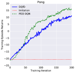
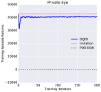
We ran experiments on a randomly selected subset of 42 Atari games. We had a human player play each game between three and twelve times. Each episode was played either until the game terminated or for 20 minutes. During game play, we logged the agent’s state, actions, rewards, and terminations. The human demonstrations range from 5,574 to 75,472 transitions per game. DQfD learns from a very small dataset compared to other similar work, as AlphaGo (?) learns from 30 million human transitions, and DQN (?) learns from over 200 million frames. DQfD’s smaller demonstration dataset makes it more difficult to learn a good representation without over-fitting. The demonstration scores for each game are shown in a table in the Appendix. Our human demonstrator is much better than PDD DQN on some games (e.g. Private Eye, Pitfall), but much worse than PDD DQN on many games (e.g. Breakout, Pong).

We found that in many of the games where the human player is better than DQN, it was due to DQN being trained with all rewards clipped to 1. For example, in Private Eye, DQN has no reason to select actions that reward 25,000 versus actions that reward 10. To make the reward function used by the human demonstrator and the agent more consistent, we used unclipped rewards and converted the rewards using a log scale: $r_{agent}=sign(r)\cdot log(1+\left|r\right|)$. This transformation keeps the rewards over a reasonable scale for the neural network to learn, while conveying important information about the relative scale of individual rewards. These adapted rewards are used internally by the all the algorithms in our experiments. Results are still reported using actual game scores as is typically done in the Atari literature (?).

Results

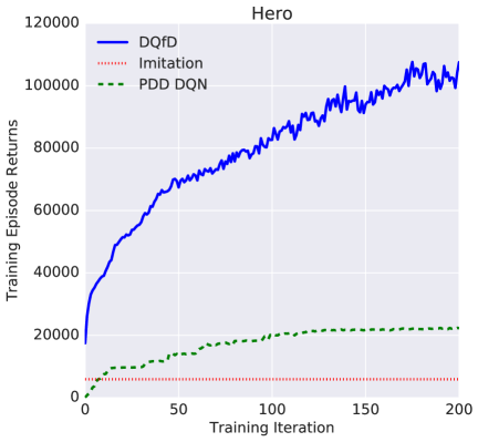
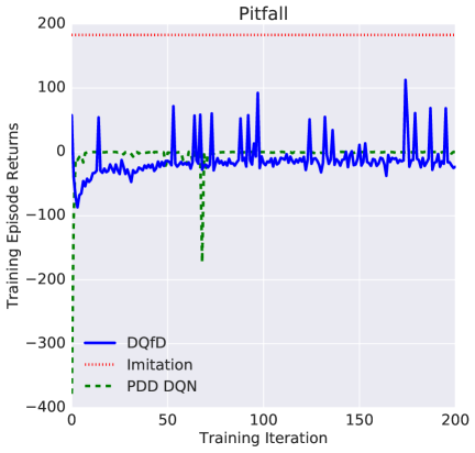
First, we show learning curves in Figure 1 for three games: Hero, Pitfall, and Road Runner. On Hero and Pitfall, the human demonstrations enable DQfD to achieve a score higher than any previously published result. Videos for both games are available at https://www.youtube.com/watch?v=JR6wmLaYuu4. On Hero, DQfD achieves a higher score than any of the human demonstrations as well as any previously published result. Pitfall may be the most difficult Atari game, as it has very sparse positive rewards and dense negative rewards. No previous approach achieved any positive rewards on this game, while DQfD’s best score on this game averaged over a 3 million step period is $394.0$.

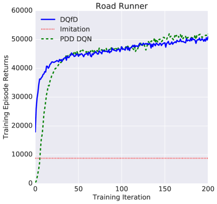
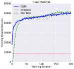
On Road Runner, agents typically learn super-human policies with a score exploit that differs greatly from human play. Our demonstrations are only human and have a maximum score of 20,200. Road Runner is the game with the smallest set of human demonstrations (only 5,574 transitions). Despite these factors, DQfD still achieves a higher score than PDD DQN for the first 36 million steps and matches PDD DQN’s performance after that.

Figure 1: On-line scores of the algorithms on the games of Hero, Pitfall, and Road Runner. On Hero and Pitfall, DQfD leverages the human demonstrations to achieve a higher score than any previously published result. The last plot shows how much more frequently the demonstration data was sampled than if data were sampled uniformly, for five different games.

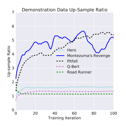
The right subplot in Figure 1 shows the ratio of how often the demonstration data was sampled versus how much it would be sampled with uniform sampling. For the most difficult games like Pitfall and Montezuma’s Revenge, the demonstration data is sampled more frequently over time. For most other games, the ratio converges to a near constant level, which differs for each game.

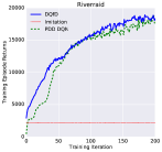
In real world tasks, the agent must perform well from its very first action and must learn quickly. DQfD performed better than PDD DQN on the first million steps on 41 of 42 games. In addition, on 31 games, DQfD starts out with higher performance than pure imitation learning, as the addition of the TD loss helps the agent generalize the demonstration data better. On average, PDD DQN does not surpass the performance of DQfD until 83 million steps into the task and never surpasses it in mean scores.

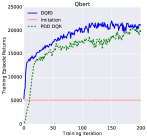
In addition to boosting initial performance, DQfD is able to leverage the human demonstrations to learn better policies on the most difficult Atari games. We compared DQfD’s scores over 200 million steps with that of other deep reinforcement learning approaches: DQN, Double DQN, Prioritized DQN, Dueling DQN, PopArt, DQN+CTS, and DQN+PixelCNN (?; ?; ?; ?; ?; ?). We took the best 3 million step window averaged over 4 seeds for the DQfD scores. DQfD achieves better scores than these algorithms on 11 of 42 games, shown in Table 1. Note that we do not compare with A3C (?) or Reactor (?) as the only published results are for human starts, and we do not compare with UNREAL (?) as they select the best hyper-parameters per game. Despite this fact, DQfD still out-performs the best UNREAL results on 10 games. DQN with count-based exploration (?) is designed for and achieves the best results on the most difficult exploration games. On the six sparse reward, hard exploration games both algorithms were run on, DQfD learns better policies on four of six games.

Game	DQfD	Prev. Best	Algorithm
Alien	4745.9	4461.4	Dueling DQN (?)
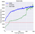
Asteroids	3796.4	2869.3	PopArt (?)
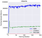
Atlantis	920213.9	395762.0	Prior. Dueling DQN (?)
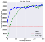
Battle Zone	41971.7	37150.0	Dueling DQN (?)
Gravitar	1693.2	859.1	DQN+PixelCNN (?)
Hero	105929.4	23037.7	Prioritized DQN (?)
Montezuma Revenge	4739.6	3705.5	DQN+CTS (?)
Pitfall	50.8	0.0	Prior. Dueling DQN (?)
Private Eye	40908.2	15806.5	DQN+PixelCNN (?)
Q-Bert	21792.7	19220.3	Dueling DQN (?)
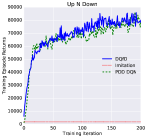
Up N Down	82555.0	44939.6	Dueling DQN (?)

Table 1: Scores for the 11 games where DQfD achieves higher scores than any previously published deep RL result using random no-op starts. Previous results take the best agent at its best iteration and evaluate it for 100 episodes. DQfD scores are the best 3 million step window averaged over four seeds, which is 508 episodes on average.

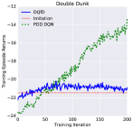
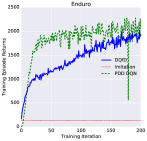
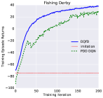
DQfD out-performs the worst demonstration episode it was given on in 29 of 42 games and it learns to play better than the best demonstration episode in 14 of the games: Amidar, Atlantis, Boxing, Breakout, Crazy Climber, Defender, Enduro, Fishing Derby, Hero, James Bond, Kung Fu Master, Pong, Road Runner, and Up N Down. In comparison, pure imitation learning is worse than the demonstrator’s performance in every game.

Figure 2: The left plots show on-line rewards of DQfD with some losses removed on the games of Montezuma’s Revenge and Q-Bert. Removing either loss degrades the performance of the algorithm. The right plots compare DQfD with three algorithms from the related work section. The other approaches do not perform as well as DQfD, particularly on Montezuma’s Revenge.

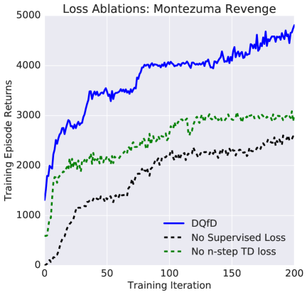
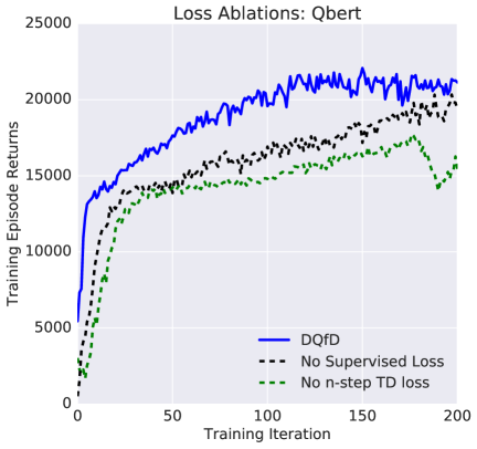
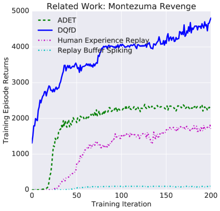
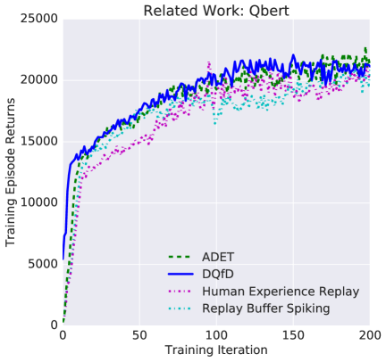
Figure 2 shows comparisons of DQfD with $\lambda_{1}$ and $\lambda_{2}$ set to 0, on two games where DQfD achieved state-of-the-art results: Montezuma’s Revenge and Q-Bert. As expected, pre-training without any supervised loss results in a network trained towards ungrounded Q-learning targets and the agent starts with much lower performance and is slower to improve. Removing the n-step TD loss has nearly as large an impact on initial performance, as the n-step TD loss greatly helps in learning from the limited demonstration dataset.

The right subplots in Figure 2 compare DQfD with three related algorithms for leveraging demonstration data in DQN:

• Replay Buffer Spiking (RBS) (?)

• Human Experience Replay (HER) (?)

• Accelerated DQN with Expert Trajectories (ADET) (?)

RBS is simply PDD DQN with the replay buffer initially full of demonstration data. HER keeps the demonstration data and mixes demonstration and agent data in each mini-batch. ADET is essentially DQfD with the large margin supervised loss replaced with a cross-entropy loss. The results show that all three of these approaches are worse than DQfD in both games. Having a supervised loss is critical to good performance, as both DQfD and ADET perform much better than the other two algorithms. All the algorithms use the exact same demonstration data used for DQfD. We included the prioritized replay mechanism and the n-step returns in all of these algorithms to make them as strong a comparison as possible.

Discussion

The learning framework that we have presented in this paper is one that is very common in real world problems such as controlling data centers, autonomous vehicles (?), or recommendation systems (?). In these problems, typically there is no accurate simulator available, and learning must be performed on the real system with real consequences. However, there is often data available of the system being operated by a previous controller. We have presented a new algorithm called DQfD that takes advantage of this data to accelerate learning on the real system. It first pre-trains solely on demonstration data, using a combination of 1-step TD, n-step TD, supervised, and regularization losses so that it has a reasonable policy that is a good starting point for learning in the task. Once it starts interacting with the task, it continues learning by sampling from both its self-generated data as well as the demonstration data. The ratio of both types of data in each mini-batch is automatically controlled by a prioritized-replay mechanism.

We have shown that DQfD gets a large boost in initial performance compared to PDD DQN. DQfD has better performance on the first million steps than PDD DQN on 41 of 42 Atari games, and on average it takes DQN 82 million steps to match DQfD’s performance. On most real world tasks, an agent may never get hundreds of millions of steps from which to learn. We also showed that DQfD out-performs three other algorithms for leveraging demonstration data in RL. The fact that DQfD out-performs all these algorithms makes it clear that it is the better choice for any real-world application of RL where this type of demonstration data is available.

In addition to its early performance boost, DQfD is able to leverage the human demonstrations to achieve state-of-the-art results on 11 Atari games. Many of these games are the hardest exploration games (i.e. Montezuma’s Revenge, Pitfall, Private Eye) where the demonstration data can be used in place of smarter exploration. This result enables the deployment of RL to problems where more intelligent exploration would otherwise be required.

DQfD achieves these results despite having a very small amount of demonstration data (5,574 to 75,472 transitions per game) that can be easily generated in just a few minutes of gameplay. DQN and DQfD receive three orders of magnitude more interaction data for RL than demonstration data. DQfD demonstrates the gains that can be achieved by adding just a small amount of demonstration data with the right algorithm. As the related work comparison shows, naively adding (e.g. only pre-training or filling the replay buffer) this small amount of data to a pure deep RL algorithm does not provide similar benefit and can sometimes be detrimental.

These results may seem obvious given that DQfD has access to privileged data, but the rewards and demonstrations are mathematically dissimilar training signals, and naive approaches to combining them can have disastrous results. Simply doing supervised learning on the human demonstrations is not successful, while DQfD learns to out-perform the best demonstration in 14 of 42 games. DQfD also out-performs three prior algorithms for incorporating demonstration data into DQN. We argue that the combination of all four losses during pre-training is critical for the agent to learn a coherent representation that is not destroyed by the switch in training signals after pre-training. Even after pre-training, the agent must continue using the expert data. In particular, the right sub-figure of Figure 1 shows that the ratio of expert data needed (selected by prioritized replay) grows during the interaction phase for the most difficult exploration games, where the demonstration data becomes more useful as the agent reaches new screens in the game. RBS shows an example where just having the demonstration data initially is not enough to provide good performance.

Learning from human demonstrations is particularly difficult. In most games, imitation learning is unable to perfectly classify the demonstrator’s actions even on the demonstration dataset. Humans may play the games in a way that differs greatly from a policy that an agent would learn, and may be using information that is not available in the agent’s state representation. In future work, we plan to measure these differences between demonstration and agent data to inform approaches that derive more value from the demonstrations. Another future direction is to apply these concepts to domains with continuous actions, where the classification loss becomes a regression loss.

Supplementary Material

Here are the parameters used for the three algorithms. DQfD used all of these parameters, while the other two algorithms only used the applicable parameters.

• Pre-training steps $k=750,000$ mini-batch updates.

• N-Step Return weight $\lambda_{1}=1.0$

• Supervised loss weight $\lambda_{2}=1.0$.

• L2 regularization weight $\lambda_{3}=10^{-5}$.

• Expert margin $l(a_{E},a)whena\neq a_{E}=0.8$.

• $\epsilon$-greedy exploration with $\epsilon=0.01$, same used by Double DQN (?).

• Prioritized replay exponent $\alpha=0.4$.

• Prioritized replay constants $\epsilon_{a}=0.001$, $\epsilon_{d}=1.0$.

• Prioritized replay importance sampling exponent $\beta_{0}=0.6$ as in (?).

• N-step returns with $n=10$.

• Target network update period $\tau=10,000$ as in  (?)

Figure 3: On-line rewards of the three algorithms on the 42 Atari games, averaged over 4 trials. Each episode is started with up to 30 radom no-op actions. Scores are from the Atari game, regardless of the internal representation of reward used by the agent.

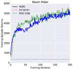
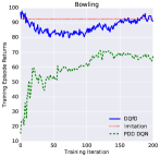
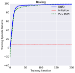
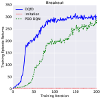
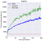
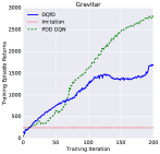
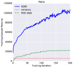
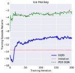
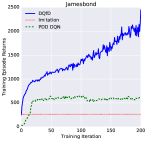
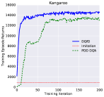
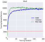
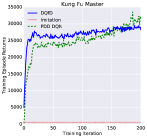
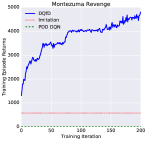
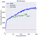
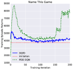
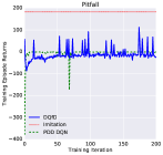
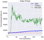
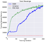
Game	Worst Demo	Best Demo	Number	Number	DQfD	PDD DQN	Imitation
	Score	Score	Transitions	Episodes	Mean Score	Mean Score	Mean Score
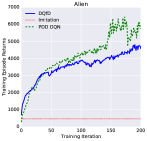
Alien	9690	29160	19133	5	4737.5	6197.1	473.9
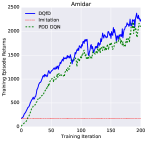
Amidar	1353	2341	16790	5	2325.0	2140.4	175.0
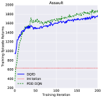
Assault	1168	2274	13224	5	1755.7	1880.9	634.4
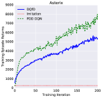
Asterix	4500	18100	9525	5	5493.6	7566.2	279.9
Asteroids	14170	18100	22801	5	3796.4	3917.6	1267.3
Atlantis	10300	22400	17516	12	920213.9	303374.8	12736.6
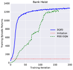
Bank Heist	900	7465	32389	7	1280.2	1240.8	95.2
Battle Zone	35000	60000	9075	5	41708.2	41993.7	14402.4
Beam Rider	12594	19844	38665	4	5173.3	5401.4	365.9
Bowling	89	149	9991	5	97.0	71.0	92.6
Boxing	0	15	8438	5	99.1	99.3	7.8
Breakout	17	79	10475	9	308.1	275.0	3.5
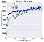
Chopper Command	4700	11300	7710	5	6993.1	6973.8	2485.7
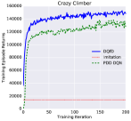
Crazy Climber	30600	61600	18937	5	151909.5	136828.2	14051.0
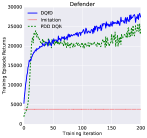
Defender	5150	18700	6421	5	27951.5	24558.8	3819.1
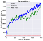
Demon Attack	1800	6190	17409	5	3848.8	3511.6	147.5
Double Dunk	-22	-14	11855	5	-20.4	-14.3	-21.4
Enduro	383	803	42058	5	1929.8	2199.6	134.8
Fishing Derby	-10	20	6388	4	38.4	28.6	-74.4
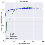
Freeway	30	32	10239	5	31.4	31.9	22.7
Gopher	2500	22520	38632	5	7810.3	12003.4	1142.6
Gravitar	2950	13400	15377	5	1685.1	2796.1	248.0
Hero	35155	99320	32907	5	105929.4	22290.1	5903.3
Ice Hockey	-4	1	17585	5	-9.6	-2.0	-13.5
James Bond	400	650	9050	5	2095.0	639.6	262.1
Kangaroo	12400	36300	20984	5	14681.5	13567.3	917.3
Krull	8040	13730	32581	5	9825.3	10344.4	2216.6
Kung Fu Master	8300	25920	12989	5	29132.0	32212.3	556.7
Montezuma’s Revenge	32300	34900	17949	5	4638.4	0.1	576.3
Ms Pacman	31781	55021	21896	3	4695.7	3684.2	692.4
Name This Game	11350	19380	43571	5	5188.3	8716.8	3745.3
Pitfall	3662	47821	35347	5	57.3	0.0	182.8
Pong	-12	0	17719	3	10.7	16.7	-20.4
Private Eye	70375	74456	10899	5	42457.2	154.3	43047.8
Q-Bert	80700	99450	75472	5	21792.7	20693.7	5133.8
River Raid	17240	39710	46233	5	18735.4	18810.0	2148.5
Road Runner	8400	20200	5574	5	50199.6	51688.4	8794.9
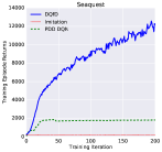
Seaquest	56510	101120	57453	7	12361.6	1862.5	195.6
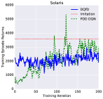
Solaris	2840	17840	28552	6	2616.8	4157.0	3589.6
Up N Down	6580	16080	10421	4	82555.0	82138.5	1816.7
Video Pinball	8409	32420	10051	5	19123.1	101339.6	10655.5
Yars’ Revenge	48361	83523	21334	4	61575.7	63484.4	4225.8

Table 2: Best and worst human demonstration scores, the number of trials and transitions collected, and average score for each algorithm on the best 3 million step window, averaged over four seeds.

References

- [Abbeel et al. 2007] Abbeel, P.; Coates, A.; Quigley, M.; and Ng, A. Y. 2007. An application of reinforcement learning to aerobatic helicopter flight. In Advances in Neural Information Processing Systems (NIPS).
- [Bellemare et al. 2013] Bellemare, M. G.; Naddaf, Y.; Veness, J.; and Bowling, M. 2013. The arcade learning environment: An evaluation platform for general agents. Journal of Artifificial Intelligence Research (JAIR) 47:253–279.
- [Brys et al. 2015] Brys, T.; Harutyunyan, A.; Suay, H.; Chernova, S.; Taylor, M.; and Nowé, A. 2015. Reinforcement learning from demonstration through shaping. In International Joint Conference on Artificial Intelligence (IJCAI).
- [Cederborg et al. 2015] Cederborg, T.; Grover, I.; Isbell, C.; and Thomaz, A. 2015. Policy shaping with human teachers. In International Joint Conference on Artificial Intelligence (IJCAI 2015).
- [Chemali and Lezaric 2015] Chemali, J., and Lezaric, A. 2015. Direct policy iteration from demonstrations. In International Joint Conference on Artificial Intelligence (IJCAI).
- [Duan et al. 2017] Duan, Y.; Andrychowicz, M.; Stadie, B. C.; Ho, J.; Schneider, J.; Sutskever, I.; Abbeel, P.; and Zaremba, W. 2017. One-shot imitation learning. CoRR abs/1703.07326.
- [Finn, Levine, and Abbeel 2016] Finn, C.; Levine, S.; and Abbeel, P. 2016. Guided cost learning: Deep inverse optimal control via policy optimization. In International Conference on Machine Learing (ICML).
- [Gruslys et al. 2017] Gruslys, A.; Gheshlaghi Azar, M.; Bellemare, M. G.; and Munos, R. 2017. The Reactor: A Sample-Efficient Actor-Critic Architecture. ArXiv e-prints.
- [Hester and Stone 2013] Hester, T., and Stone, P. 2013. TEXPLORE: Real-time sample-efficient reinforcement learning for robots. Machine Learning 90(3).
- [Ho and Ermon 2016] Ho, J., and Ermon, S. 2016. Generative adversarial imitation learning. In Advances in Neural Information Processing Systems (NIPS).
- [Hosu and Rebedea 2016] Hosu, I.-A., and Rebedea, T. 2016. Playing atari games with deep reinforcement learning and human checkpoint replay. In ECAI Workshop on Evaluating General Purpose AI.
- [Jaderberg et al. 2016] Jaderberg, M.; Mnih, V.; Czarnecki, W. M.; Schaul, T.; Leibo, J. Z.; Silver, D.; and Kavukcuoglu, K. 2016. Reinforcement learning with unsupervised auxiliary tasks. CoRR abs/1611.05397.
- [Kim et al. 2013] Kim, B.; Farahmand, A.; Pineau, J.; and Precup, D. 2013. Learning from limited demonstrations. In Advances in Neural Information Processing Systems (NIPS).
- [Lakshminarayanan, Ozair, and Bengio 2016] Lakshminarayanan, A. S.; Ozair, S.; and Bengio, Y. 2016. Reinforcement learning with few expert demonstrations. In NIPS Workshop on Deep Learning for Action and Interaction.
- [LeCun, Bengio, and Hinton 2015] LeCun, Y.; Bengio, Y.; and Hinton, G. 2015. Deep learning. Nature 521(7553):436–444.
- [Levine et al. 2016] Levine, S.; Finn, C.; Darrell, T.; and Abbeel, P. 2016. End-to-end training of deep visuomotor policies. Journal of Machine Learning (JMLR) 17:1–40.
- [Lipton et al. 2016] Lipton, Z. C.; Gao, J.; Li, L.; Li, X.; Ahmed, F.; and Deng, L. 2016. Efficient exploration for dialog policy learning with deep BBQ network & replay buffer spiking. CoRR abs/1608.05081.
- [Mnih et al. 2015] Mnih, V.; Kavukcuoglu, K.; Silver, D.; Rusu, A. A.; Veness, J.; Bellemare, M. G.; Graves, A.; Riedmiller, M.; Fidjeland, A. K.; Ostrovski, G.; Petersen, S.; Beattie, C.; Sadik, A.; Antonoglou, I.; King, H.; Kumaran, D.; Wierstra, D.; Legg, S.; and Hassabis, D. 2015. Human-level control through deep reinforcement learning. Nature 518(7540):529–533.
- [Mnih et al. 2016] Mnih, V.; Badia, A. P.; Mirza, M.; Graves, A.; Lillicrap, T.; Harley, T.; Silver, D.; and Kavukcuoglu, K. 2016. Asynchronous methods for deep reinforcement learning. In International Conference on Machine Learning, 1928–1937.
- [Ostrovski et al. 2017] Ostrovski, G.; Bellemare, M. G.; van den Oord, A.; and Munos, R. 2017. Count-based exploration with neural density models. CoRR abs/1703.01310.
- [Piot, Geist, and Pietquin 2014a] Piot, B.; Geist, M.; and Pietquin, O. 2014a. Boosted bellman residual minimization handling expert demonstrations. In European Conference on Machine Learning (ECML).
- [Piot, Geist, and Pietquin 2014b] Piot, B.; Geist, M.; and Pietquin, O. 2014b. Boosted and Reward-regularized Classification for Apprenticeship Learning. In International Conference on Autonomous Agents and Multiagent Systems (AAMAS).
- [Ross, Gordon, and Bagnell 2011] Ross, S.; Gordon, G. J.; and Bagnell, J. A. 2011. A reduction of imitation learning and structured prediction to no-regret online learning. In International Conference on Artificial Intelligence and Statistics (AISTATS).
- [Schaal 1996] Schaal, S. 1996. Learning from demonstration. In Advances in Neural Information Processing Systems (NIPS).
- [Schaul et al. 2016] Schaul, T.; Quan, J.; Antonoglou, I.; and Silver, D. 2016. Prioritized experience replay. In Proceedings of the International Conference on Learning Representations, volume abs/1511.05952.
- [Shani, Heckerman, and Brafman 2005] Shani, G.; Heckerman, D.; and Brafman, R. I. 2005. An mdp-based recommender system. Journal of Machine Learning Research 6:1265–1295.
- [Silver et al. 2016] Silver, D.; Huang, A.; Maddison, C. J.; Guez, A.; Sifre, L.; van den Driessche, G.; Schrittwieser, J.; Antonoglou, I.; Panneershelvam, V.; Lanctot, M.; Dieleman, S.; Grewe, D.; Nham, J.; Kalchbrenner, N.; Sutskever, I.; Lillicrap, T.; Leach, M.; Kavukcuoglu, K.; Graepel, T.; and Hassabis, D. 2016. Mastering the game of Go with deep neural networks and tree search. Nature 529:484––489.
- [Suay et al. 2016] Suay, H. B.; Brys, T.; Taylor, M. E.; and Chernova, S. 2016. Learning from demonstration for shaping through inverse reinforcement learning. In International Conference on Autonomous Agents and Multiagent Systems (AAMAS).
- [Subramanian, Jr., and Thomaz 2016] Subramanian, K.; Jr., C. L. I.; and Thomaz, A. 2016. Exploration from demonstration for interactive reinforcement learning. In International Conference on Autonomous Agents and Multiagent Systems (AAMAS).
- [Sun et al. 2017] Sun, W.; Venkatraman, A.; Gordon, G. J.; Boots, B.; and Bagnell, J. A. 2017. Deeply aggrevated: Differentiable imitation learning for sequential prediction. CoRR abs/1703.01030.
- [Sutton and Barto 1998] Sutton, R. S., and Barto, A. G. 1998. Introduction to reinforcement learning. MIT Press.
- [Syed and Schapire 2007] Syed, U., and Schapire, R. E. 2007. A game-theoretic approach to apprenticeship learning. In Advances in Neural Information Processing Systems (NIPS).
- [Syed, Bowling, and Schapire 2008] Syed, U.; Bowling, M.; and Schapire, R. E. 2008. Apprenticeship learning using linear programming. In International Conference on Machine Learning (ICML).
- [Taylor, Suay, and Chernova 2011] Taylor, M.; Suay, H.; and Chernova, S. 2011. Integrating reinforcement learning with human demonstrations of varying ability. In International Conference on Autonomous Agents and Multiagent Systems (AAMAS).
- [van Hasselt et al. 2016] van Hasselt, H. P.; Guez, A.; Hessel, M.; Mnih, V.; and Silver, D. 2016. Learning values across many orders of magnitude. In Advances in Neural Information Processing Systems (NIPS).
- [van Hasselt, Guez, and Silver 2016] van Hasselt, H.; Guez, A.; and Silver, D. 2016. Deep reinforcement learning with double Q-learning. In AAAI Conference on Artificial Intelligence (AAAI).
- [Wang et al. 2016] Wang, Z.; Schaul, T.; Hessel, M.; van Hasselt, H.; Lanctot, M.; and de Freitas, N. 2016. Dueling network architectures for deep reinforcement learning. In International Conference on Machine Learning (ICML).
- [Watter et al. 2015] Watter, M.; Springenberg, J. T.; Boedecker, J.; and Riedmiller, M. A. 2015. Embed to control: A locally linear latent dynamics model for control from raw images. In Advances in Neural Information Processing (NIPS).