Determination of the density and temperature dependence of the shear viscosity of a unitary Fermi gas based on hydrodynamic flow

Abstract

We determine the shear viscosity of the ultracold Fermi gas at unitarity in the normal phase using hydrodynamic expansion data. The analysis is based on a generalized fluid dynamic framework which ensures a smooth transition between the fluid dynamic core of the cloud and the ballistic corona. We use expansion data taken by Joseph et al. Joseph:2014 and measurements of the equation of state by Ku et al. Ku:2011 . We find that the shear viscosity to particle density ratio just above the critical temperature is $\left.\eta/n\right|_{T_{c}}=0.41\pm 0.11$. We also obtain evidence that the shear viscosity to entropy density ratio has a minimum slightly above $T_{c}$ with $\left.\eta/s\right|_{\it min}=0.50\pm 0.10$.

Introduction: The dilute Fermi gas at unitarity is a very attractive physical system for studying the transport properties of strongly correlated quantum fluids Schafer:2009dj ; Adams:2012th ; Schaefer:2014awa . From a theoretical point of view the unitary Fermi gas is a parameter-free, scale invariant, and intrinsically quantum mechanical many-body system. A lot of interest has centered on the question of how close the viscosity to entropy density ratio of this system comes to the proposed string theory bound $\eta/s=\hbar/(4\pi k_{B})$ Kovtun:2004de . Experimentally, the unitary Fermi gas can be realized in dilute atomic gases using Feshbach resonances Bloch:2007 ; Giorgini:2008 . The experimental control provided by Feshbach resonances implies that we can study the transition from the strongly correlated unitary Fermi gas to weakly coupled Bose and Fermi gases.

In this work we focus on the problem of extracting the shear viscosity of the unitary Fermi gas from experiments with trapped ultracold gases Kinast:2004b ; Schafer:2007pr ; Turlapov:2007 ; Bruun:2007 ; Cao:2010wa ; Elliott:2013b ; Joseph:2014 ; Elliott:2013 ; Brewer:2015hua . Our main interest is in the low temperature regime, where the density dependence of the shear viscosity is relevant, and the minimum of $\eta/s$ is likely to be achieved. There are two main types of experiments that are relevant to this problem. The first class involves measuring the damping rate of collective excitations, and the second focuses on the expansion of the cloud after removing the trapping potential. From a theoretical perspective the damping experiments would appear to be more attractive, because even a very small viscosity leads to a clear signature in the exponential decay of the collective mode. In practice, however, the expansion experiments take place in a cleaner environment and have achieved greater accuracy. In an expansion experiment what is observed is the time evolution of the aspect ratio of the cloud. Hydrodynamic pressure gradients accelerate the cloud along the short direction, so that the aspect ratio increases as a function of time. Viscosity counteracts the pressure gradients, and slows the growth of the aspect ratio. These flow experiments are very similar to elliptic flow experiments in relativistic heavy ion physics Ackermann:2000tr ; Adler:2003kt ; Aamodt:2010pa .

The main difficulty in analyzing these experiments is that the viscosity $\eta(n,T)$ is a local quantity that varies with the density $n$ and temperature $T$ of the cloud, while the observed aspect ratio is a global property of the trapped gas. This means that the dependence of the data on initial cloud energy, particle number, and expansion time has to be unfolded to determine $\eta(n,T)$. An even more significant problem is that the viscosity is a parameter that appears in the fluid dynamic description of the cloud. However, fluid dynamics breaks down in the dilute, dissipative corona of the gas.

We have recently made significant progress in dealing with the physics of the dilute corona. We have introduced a new method, anisotropic fluid dynamics Bluhm:2015raa ; Florkowski:2010 ; Martinez:2010sc , that takes into account the effects of non-hydrodynamic modes. These modes quickly relax in the dense part of the cloud so that Navier-Stokes fluid dynamics is recovered. In the dilute corona non-hydrodynamic modes ensure a smooth transition to a free-streaming, ballistic expansion. We have checked numerically that anisotropic fluid dynamics reproduces the Navier-Stokes equation in the dense limit Bluhm:2015raa as well as numerical solutions of the Boltzmann equation in the dilute regime Pantel:2014jfa ; Bluhm:2015bzi . We have also shown that the anisotropic fluid dynamics, combined with the kinetic theory prediction for the shear viscosity $\eta=15/(32\sqrt{\pi})(mT)^{3/2}$ Bruun:2005 , reproduces the high temperature expansion data obtained in Cao:2010wa . Note that here and in the remainder of the paper we set $\hbar$ and $k_{B}$ equal to unity.

In this work we extend our studies to lower temperature. For this purpose we fit the expansion data to a systematic expansion of the viscosity in powers of the density. We show that the data clearly demand that the shear viscosity has non-trivial density dependence. We also show that the density dependence in the normal phase is quite smooth, and that the existing data place strong constraints on $\eta/n$ near $T_{c}$. This study requires several refinements of our previous work. We extend the fluid dynamic analysis to three dimensional systems with no axial symmetry. We include an accurate parametrization of the measured equation of state, and a more general functional form of the shear viscosity.

Anisotropic fluid dynamics: In this section we briefly summarize the anisotropic fluid dynamics method Bluhm:2015raa . The fluid dynamical variables that characterize a non-relativistic fluid in the normal phase are the mass density $\rho$, the momentum density $\vec{\pi}=\rho\vec{u}$, and the energy density ${\cal E}$. The equations of motion follow from the conservation laws

$$D_{0}\rho = -\rho\,\vec{\nabla}\cdot\vec{u}\,,$$ (1)

$$D_{0}u_{i} = -\frac{1}{\rho}\,\nabla_{j}\left(\delta_{ij}P+\delta\Pi_{ij}\right)\,,$$ (2)

$$D_{0}\epsilon = -\frac{1}{\rho}\,\nabla_{i}\left(u_{i}P+\delta\jmath^{\cal E}_{i}\right)\,.$$ (3)

Here, we defined the comoving time derivative $D_{0}=\partial_{0}+\vec{u}\cdot\vec{\nabla}$, the energy per mass $\epsilon={\cal E}/\rho$, and the pressure $P$. We also introduce the energy density in the rest frame of the fluid, ${\cal E}^{0}={\cal E}-\frac{1}{2}\rho\vec{u}^{\,2}$. In order for the equations to close we have to provide an equation of state $P=P({\cal E}^{0},\rho)$, and constitutive equations for the dissipative stresses $\delta\Pi_{ij}$ and the dissipative energy current $\delta\jmath^{\cal E}_{i}$. For the unitary Fermi gas scale invariance implies that $P=\frac{2}{3}{\cal E}^{0}$.

In the Navier-Stokes approximation the dissipative stresses are expanded to first order in gradients of the thermodynamic variables. We get $\delta\Pi_{ij}=-\eta\sigma_{ij}$ with

$$\sigma_{ij}=\nabla_{i}u_{j}+\nabla_{j}u_{i}-\frac{2}{3}\delta_{ij}\vec{\nabla}\cdot\vec{u}$$ (4)

and $\delta\jmath^{\cal E}_{i}=u_{j}\delta\Pi_{ij}$. Scale invariance implies that the bulk viscosity vanishes. We have also used the fact that in expansion experiments the effects of heat conduction are of higher order in the gradient expansion. This is related to the fact that the initial temperature is constant, and that the expansion of an ideal gas preserves the isothermal nature of the temperature profile Schafer:2010dv .

In anisotropic fluid dynamics we treat the components of the dissipative stress tensor as independent fluid dynamical variables. The symmetries of the trap imply that the stresses are diagonal. We define anisotropic components of the pressure, $P_{a}$ for $a=1,2,3$, and define

$$\delta\Pi_{ij}={\rm diag}(\Delta P_{1},\Delta P_{2},\Delta P_{3}),$$ (5)

where $\Delta P_{a}=P_{a}-P$. We also define anisotropic components of the energy density ${\cal E}_{a}$ such that ${\cal E}=\sum_{a}{\cal E}_{a}$. The anisotropic components of the energy per mass satisfy the equation of motion Bluhm:2015raa

$$D_{0}\epsilon_{a}=-\frac{1}{\rho}\nabla_{i}\left[\delta_{ia}u_{i}P+(\delta\jmath^{\cal E}_{a})_{i}\right]-\frac{P}{2\eta\rho}\,\Delta P_{a}\,,$$ (6)

where $\epsilon_{a}={\cal E}_{a}/\rho$ and $(\delta\jmath^{\cal E}_{a})_{i}=\delta_{ia}u_{j}\delta\Pi_{ij}$. The anisotropic pressure is related to the anisotropic energy density by an equation of state. In the case of a scale invariant fluid we have $P_{a}({\cal E}^{0}_{a})=2\,{\cal E}^{0}_{a}$ with ${\cal E}^{0}_{a}={\cal E}_{a}-\frac{1}{2}\rho u_{a}^{2}$. Then $P=\frac{1}{3}\sum_{a}P_{a}$ satisfies the isotropic equation of state, and equ. (6) gives the isotropic equation of energy conservation equ. (3) when summed over $a$. In our previous work we have described a three dimensional fluid dynamics code that solves equ. (1)-(3) and equ. (6) Schafer:2010dv ; Bluhm:2015raa . This code is based on the PPM scheme of Colella and Woodward Colella:1984 ; Blondin:1993 .

We have shown that in the limit of small viscosity, $\eta(\vec{\nabla}\cdot\vec{u})\ll P$, the anisotropic pressure terms relax to the viscous stress tensor in Navier Stokes theory, $\Delta P_{a}=-\eta\sigma_{aa}$. We observe that in the opposite limit, that of very large viscosity, equ. (6) becomes a conservation law. This conservation law ensures that anisotropic fluid dynamics reproduces the free streaming limit. Finally, we have checked that anisotropic fluid dynamics provides a very accurate representation of numerical solutions of the Boltzmann equation in the limit that two-body scattering dominates Bluhm:2015bzi .

In general the viscosity is a function of density and temperature. In the unitary limit scale invariance implies that $\eta(n,T)=(mT)^{3/2}f(n\lambda^{3})$, where $\lambda=[(2\pi)/(mT)]^{1/2}$ is the de Broglie wave length. In this work we will expand the function $f(x)$ in powers of the diluteness of the gas

$$\eta(n,T)=\eta_{0}(mT)^{3/2}\left\{1+\eta_{2}\left(n\lambda^{3}\right)+\eta_{3}\left(n\lambda^{3}\right)^{2}+\ldots\right\}\,.$$ (7)

We note that the leading term is purely a function of temperature, the first correction is solely a function of density, and higher order terms depend on increasing powers of the density. In general this expansion is not expected to be useful near $T_{c}$, but we will show that terms that scale as $(n\lambda^{3})^{2}$ and higher are surprisingly small.

Experimental parameters: We will analyze the expansion data reported in Joseph:2014 . This work represents the most complete set of elliptic flow measurements for the unitary Fermi gas over a wide range of temperatures currently available. The gas is released from a harmonic trap $V_{\it ext}=\frac{1}{2}m\omega_{i}^{2}x_{i}^{2}$ with trap frequencies $(\omega_{x},\omega_{y},\omega_{z})=(2\pi)(2210,830,64.3)$ Hz. After the optical trap is turned off there is a residual magnetic bowl characterized by $\omega_{\it mag}=2\pi\cdot 21.5\,{\it Hz}$. The total energy per particle of the gas varies between $E/(NE_{F})=(0.56-1.91)$. Here, $N$ is the number of particles and $E_{F}\equiv(3N)^{1/3}\bar{\omega}$, where $\bar{\omega}$ is the geometric mean of the trap frequencies. The energy and temperature of the cloud are extracted using absorption images and an equation of state ${\cal E}^{0}(n,T)$. We describe a parametrization of the equation of state measured by the MIT group Ku:2011 in the Appendix. Based on this equation of state we find that the critical energy where superfluidity occurs at the center of the trap is $E/(NE_{F})=0.70$. In the high temperature limit many relations simplify. For example, the total cloud energy is given by $E=3NT$. We will characterize the initial temperature using the dimensionless ratio $T/T_{F}$, where $T_{F}=E_{F}$.

Figure 1: Aspect ratio $A_{R}=\sigma_{x}/\sigma_{y}$ at $t^{*}=1.2\,{\it msec}$ as a function of the energy $E/(NE_{F})$ of the cloud. Data (gray points) compared to hydrodynamic fits based on the equation of state of a free gas. The solid red line corresponds to the shear viscosity $\eta=\eta_{0}(mT)^{3/2}$ predicted by kinetic theory, and the dashed and dotted line show the $\pm 25\%$ and $\pm 50\%$ range in $\eta_{0}$. The thick green line is the best fit to the high energy data, corresponding to $\eta_{0}=0.301$.

Figure 2: Aspect ratio $A_{R}=\sigma_{x}/\sigma_{y}$ at $t^{*}=1.2\,{\it msec}$ as a function of the energy $E/(NE_{F})$ of the cloud. Data (gray points) compared to hydrodynamic fits based on the measured equation of state. The red short-dashed line shows the high temperature fit, the blue dashed line includes density corrections, and the green solid line contains a density squared term.

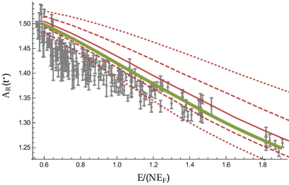
Scaling of the aspect ratio with the initial energy: Expansion experiments measure the time evolution of the aspect ratio $A_{R}(t)$ for different initial energies and particle numbers. The experiment of Joseph et al. Joseph:2014 focuses on the ratio $\sigma_{x}/\sigma_{y}$, which reaches its asymptotic behavior more quickly than $\sigma_{x}/\sigma_{z}$ or $\sigma_{y}/\sigma_{z}$. The radii $\sigma_{i}$ are determined from a Gaussian fit to two-dimensional absorption images. As noted in Pantel:2014jfa it is important to follow this definition when analyzing the data using transport theory. In particular, there is a significant difference between the ratio of rms radii, $\sqrt{\langle x^{2}\rangle}/\sqrt{\langle y^{2}\rangle}$, and the ratio of Gaussian fit radii, $\sigma_{x}/\sigma_{y}$. This is the case even if the initial density distribution is a Gaussian.

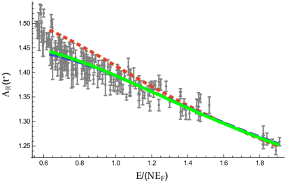
Joseph et al. observed that the main information about the density and temperature dependence of $\eta(n,T)$ is not carried by the time dependence of $A_{R}(t)$ for fixed initial energy, but by the dependence of $A_{R}(t^{*})$ at a fixed time $t^{*}$ on the initial energy. In Fig. 1 we show $A_{R}(t^{*})=\sigma_{x}/\sigma_{y}$ as a function of $E/(NE_{F})$ at $t^{*}=1.2\,{\it msec}$. Note that the plot covers a fairly narrow range in $A_{R}$. Individual data points are more accurate than previously published data, which spanned a much larger range in aspect ratio.

A difficulty in interpreting the results is that the data points correspond to a range of particle numbers. The data are clustered around a mean $\bar{N}=1.94\cdot 10^{5}$, and the variance in $N^{1/3}$, which is relevant to the effective viscosity, is about 7%. We show all the data points on the same plot, but when performing hydrodynamic fits we use the correct number of particles for each individual data point.

Figure 1 shows a fit to the data based on the high temperature theory only. This means that we use the free gas equation of state, and only the first coefficient, $\eta_{0}$, in the virial expansion of the shear viscosity. The best fit to the high temperature data gives $\eta_{0}=0.301$ which is somewhat higher than the value $\eta_{0}=0.264$ predicted by kinetic theory. The best fit value shifts slightly if the full equation of state is used, but the shape of $A_{R}(t^{*})$ as a function of $E/(NE_{F})$ does not change. We observe that the data at lower energy clearly demand a more complicated functional form of the shear viscosity.

Figure 3: In this figure we show the reconstructed ratio $\eta/n$ as a function of $T/T_{F}^{\it loc}$ for a homogeneous gas. The local Fermi temperature is defined as $T_{F}^{\it loc}=k_{F}^{2}/(2m)$ where $k_{F}$ is defined via the density of the gas, $n=k_{F}^{3}/(3\pi^{2})$. The red line shows the density expansion together with the error band described in the text. The curves terminate at $T_{c}$. The gray dots show the reconstruction obtained in Joseph:2014 , and the dashed line shows the $T$-matrix calculation of Enss et al. Enss:2010qh .

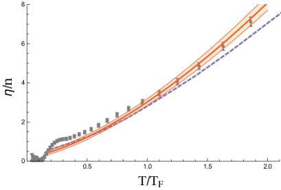
Figure 2 shows a fit to the data above the superfluid transition based on the full equation of state and an expansion of the shear viscosity up to second order in density. The best fit is

$$\eta_{0}=0.265\pm 0.02\,,\hskip 28.45274pt\eta_{2}=0.060\pm 0.02\,,$$ (8)

and $\eta_{3}=-(2\pm 8)\cdot 10^{-4}$. We observe that the $n^{2}$ coefficient is consistent with zero within error bars. We also find that the fit is stable with respect to including higher order terms in $n$. The $\chi^{2}/N_{\it dof}$ of the fit is of order unity, indicating that this simple model provides a very good representation of all the data in the entire regime above the superfluid phase transition. We note that $\eta_{0}$ agrees to better than 1% with the kinetic theory prediction $\eta_{0}=0.264$.

Figure 4: Same as Fig. 3, zooming in on the low temperature regime. Our analysis (red band) is compared to the results (gray points) obtained in Joseph:2014 , the $T$-matrix calculation (dashed line) of Enss et al. Enss:2010qh , and the lattice calculation (green band) of Wlazlowski et al. Wlazlowski:2013owa .

Conclusions: Our determination of $\eta/n$ for the homogeneous Fermi gas is shown in Figs. 3 and 4. The result is shown as a function of $T/T_{F}^{\it loc}$, where $T_{F}^{\it loc}=k_{F}^{2}/(2m)$ is the local Fermi temperature of the gas. The best fit to the data, shown as the thick red line in Fig. 3, is

$$\eta/n=2.773\,x^{3/2}+0.251-0.0013\,x^{-3/2}\,,$$ (9)

where $x=T/T_{F}^{\it loc}$. The coefficients in equ. (9) are given by the central values of $\eta_{0},\eta_{1},\eta_{2}$ normalized by the density $n$. The local Fermi momentum $k_{F}$ is defined in terms of the density of the gas, $n=k_{F}^{3}/(3\pi^{2})$. We show the reconstruction for temperatures above the critical temperature $T_{c}=0.167(13)T_{F}^{\it loc}$ Ku:2011 . We find that the value of the viscosity at $T_{c}$ is $\eta/n|_{T_{c}}=0.41\pm 0.11$. We have not attempted to reconstruct the shear viscosity below $T_{c}$, since a proper treatment of this regime requires superfluid hydrodynamics.

Figure 5: Low temperature behavior of the shear viscosity to entropy density ratio $\eta/s$ as a function of $T/T_{F}^{\it loc}$. Our analysis (red band) is compared to the high and low temperature predictions from kinetic theory, see Bruun:2005 ; Rupak:2007vp .

For comparison the gray data points show the reconstructed values of $\eta/n$ obtained in the experimental work of Joseph et al. Joseph:2014 . These results are based on the same expansion data, but involve a number of assumptions . The main assumption is that there is a critical radius $R^{\it crit}_{i}$ so that the atomic cloud inside this radius can be described as a viscous fluid, and the particles outside the radius are a non-interacting gas. The critical radius is assumed to be a constant fraction of the cloud size. The overall constant is adjusted to reproduce the expected behavior of the high temperature viscosity, $\eta\sim\eta_{0}(mT)^{3/2}$. This implies that the agreement of the data points with kinetic theory for large $T/T_{F}^{\it loc}$ is not a result, but an input. In contrast, the agreement of our reconstruction with kinetic theory is a non-trivial result. There is some discrepancy between the two reconstructions in the regime $T=(0.2-1.0)T_{F}^{\it loc}$. In this regime our result for $\eta/n$ is systematically lower. This makes sense if one assumes that as the temperature is lowered and the viscosity drops the effective fluid radius increases. This implies that assuming a constant radius of the fluid core leads to an overestimate of the viscosity. It is interesting that directly at $T_{c}$ the two reconstructions agree.

We also show the $T$-matrix calculation of Enss et al. Enss:2010qh , which agrees quite well with our reconstructed viscosity near $T_{c}$. It will be interesting to study the physical consequences of this result, for example possible implications for quasi-particle models. We also show the lattice calculation of Wlazlowski et al. Wlazlowski:2013owa . The calculation does not match the shape of our reconstruction, and has a substantially smaller $\left.\eta/n\right|_{T_{c}}$.

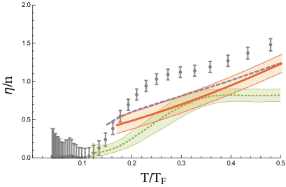
Finally, Fig. 5 shows the ratio of shear viscosity to entropy density, based on our reconstruction of $\eta/n$ and the measurement of $s/n$ by the MIT group Ku:2011 . The result is compared to high and low temperature predictions for $\eta/s$ in kinetic theory Bruun:2005 ; Rupak:2007vp . We find a shallow minimum of $\left.\eta/s\right|_{\it min}=0.50\pm 0.10$ slightly above $T_{c}$. The minimum is related to the fact that the entropy per particle drops siginificantly as $T_{c}$ is approached from above, whereas no structure is seen in $\eta/n$. We note that at present we can only weakly exclude (at about 1$\sigma$) a minimum in $\eta/s$ at or below $T_{c}$. A minimum in $\eta/s$ above $T_{c}$ was predicted in Zwerger:2016xma , but is in tension with the Monte Carlo data in Wlazlowski:2013owa .

Acknowledgments: This work was supported in parts by the US Department of Energy grant DE-FG02-03ER41260. The work of M. Bluhm is funded by the European Union’s Horizon 2020 research and innovation program under the Marie Skłodowska Curie grant agreement No 665778 via the National Science Center, Poland, under grant Polonez UMO-2016/21/P/ST2/04035. We would like to thank James Joseph and John Thomas for many useful discussions, and for providing us with the data in Joseph:2014 . We thank Martin Zwierlein for providing us with the data in Ku:2011 .

Appendix A Choice of units and scaling with the number of particles

The fluid dynamic analysis employs a set of dimensionless variables. The time scale for the expansion is set by the inverse geometric mean of the trap frequencies, $t_{0}={\bar{\omega}}^{-1}=3.24534\cdot 10^{-4}\,{\it sec}$, and a dimensionless time variable is given by $\bar{t}=t/t_{0}$. We will also use dimensionless frequency variables $\tilde{\omega}_{i}=\omega_{i}/\bar{\omega}$. In the present case $(\tilde{\omega}_{x},\tilde{\omega}_{y},\tilde{\omega}_{z})=(4.506,1.692,0.131)$. The unit of distance is

$$x_{0}=\left[\frac{2}{3}\frac{(3N)^{1/3}}{m\bar{\omega}}\right]^{1/2}\,.$$ (10)

For a typical number of atoms, $N=2\cdot 10^{5}$, this is $x_{0}=13.8\,\mu{\it m}$. The unit of density is $n_{0}=x_{0}^{-3}$, the unit of temperature is $T_{0}=m\bar{\omega}^{2}x_{0}^{2}$, and the unit of pressure is $P_{0}=n_{0}T_{0}=m\bar{\omega}^{2}x_{0}^{-1}$. The unit of viscosity is $\eta_{0}=m\bar{\omega}/x_{0}$. We can construct dimensionless variables by considering appropriate ratios. The dimensionless temperature is $\bar{T}=T/T_{0}$. In the case of densities we also normalize by the density $n^{B}$ of a Boltzmann gas at the center of the trap. We have $\bar{n}=n/n^{\it B}(0)$, $\bar{P}=(P/P_{0})(n_{0}/n^{\it B}(0))$ and $\bar{\eta}=(\eta/\eta_{0})(n_{0}/n^{\it B}(0))$ with

$$\frac{n^{\it B}(0)}{n_{0}}=\frac{N}{(3\pi)^{3/2}}\left(\frac{T_{F}}{T}\right)^{3/2}\,.$$ (11)

These rescalings preserve simple relations such as the equation of state of a free gas $P=nT$, which becomes $\bar{P}=\bar{n}\bar{T}$. In scaled variables the initial condition in the high temperature limit takes a very simple form. We have

$$\bar{n}(\bar{x})=\exp[-(\tilde{\omega}_{i}^{2}\bar{x}_{i}^{2})/(2\bar{T})],$$ (12)

which is independent of the number of particles $N$. Initial density and pressure profiles that follow from the full equation of state are discussed in Sec. B below. The exact profiles are also independent of $N$.

The dependence on the number of particles enters through viscous corrections. The density expansion of the viscosity can be written as

$$\eta=\alpha_{T}(mT)^{3/2}+\alpha_{n}n+\alpha_{n^{2}}n^{2}(mT)^{-3/2}+\ldots,$$ (13)

where the coefficients $\alpha_{i}$ are related to $\eta_{i}$ by

$$\alpha_{T} = \eta_{0}\,,$$ (14)

$$\alpha_{n} = (2\pi)^{3/2}\eta_{0}\eta_{2}\,,$$ (15)

$$\alpha_{n^{2}} = (2\pi)^{3}\eta_{0}\eta_{3}\,.$$ (16)

In dimensionless variables we write $\bar{\eta}=\bar{\alpha}_{T}\bar{T}^{3/2}+\bar{\alpha}_{n}\bar{n}+\bar{\alpha}_{n^{2}}\bar{T}^{-3/2}\bar{n}^{2}+\ldots$, where

$$\bar{\alpha}_{T} = \frac{4\pi^{3/2}\alpha_{T}}{3(3N)^{1/3}}\left(\frac{3T}{T_{F}}\right)^{3/2}\,,$$ (17)

$$\bar{\alpha}_{n} = \frac{3\alpha_{n}}{2(3N)^{1/3}}\,,$$ (18)

$$\bar{\alpha}_{n^{2}} = \frac{27\alpha_{n^{2}}}{16\pi^{3/2}(3N)^{1/3}}\left(\frac{T_{F}}{3T}\right)^{3/2}\,.$$ (19)

We observe that at fixed $T/T_{F}$ all terms in the density expansion of the viscosity scale as $N^{-1/3}$. This makes it relatively easy to analyze data taken at different values of $N$.

In the manuscript we provide a simple fit to the viscosity which is of the form $\eta/n=a_{0}x^{3/2}+a_{1}+a_{2}x^{-3/2}$, where $x=T/T_{F}^{\it loc}$ with $T_{F}^{\it loc}=k_{F}^{2}/(2m)$ and $n=k_{F}^{3}/(3\pi^{2})$. This result is useful for comparing the fluid dynamic fits with theoretical and numerical results in the literature. The coefficients $a_{i}$ are given by

$$a_{0} = \alpha_{T}\,\frac{3\pi^{2}}{2^{3/2}}\,,$$ (20)

$$a_{1} = \alpha_{n}\,,$$ (21)

$$a_{2} = \alpha_{n^{2}}\,\frac{2^{3/2}}{3\pi^{2}}\,.$$ (22)

Appendix B Equation of state

Figure 6: Ratio of the full pressure over the pressure of a free gas, as a function of inverse fugacity, from Fig. 4 of Ku:2011 . The points show the data points, and the line is the fit function discussed in the text. The dashed line shows a fit to the data of Nascimbene et al. Nascimbene:2009 . The critical point corresponds to $\zeta\simeq 0.08$.

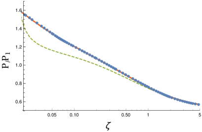
The high temperature analysis in Bluhm:2015bzi was based on the non-interacting equation of state $P=nT$. In order to perform a reliable determination of $\eta(n,T)$ at lower temperature we need to use a realistic equation of state. It is interesting to note that the viscous fluid dynamics evolution does not make use of $P(n,T)$, it only uses the exact relation $P=\frac{2}{3}{\cal E}$. However, the equation of state is needed to convert the experimentally measured quantity $E/(NE_{F})$ to an initial temperature $T/T_{F}$, and to determine the initial density and pressure profile $n(x,0)$, $P(x,0)$. The equation of state is also needed to determine the local temperature that enters into the shear viscosity $\eta(n,T)$.

In the following we will discuss a simple parametrization of the equation of state measured by the MIT group Ku:2011 . The method we have used is described in Appendix A of Schafer:2010dv , where it was used to parameterize the equation of state published by Nascimbene et al. Nascimbene:2009 . A similar fit was also employed in Romatschke:2012sf . We write the pressure as

$$P(\zeta)=h(\zeta)P_{1}(\zeta),\hskip 14.22636ptP_{1}(\zeta)=-T\lambda^{-3}{\it Li}_{5/2}(-\zeta^{-1})\,,$$ (23)

where $\zeta=\exp(-\mu/T)$ is the inverse fugacity, $P_{1}$ is the pressure of a single component non-interacting Fermi gas, $\lambda=[(2\pi)/(mT)]^{1/2}$ is the thermal de Broglie wave length, and ${\it Li}_{p}$ is the Polylogarithm of order $p$. We also define

$$f(\zeta)=-h(\zeta){\it Li}_{5/2}(-\zeta^{-1})\,.$$ (24)

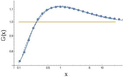
Numerical data for $h(\zeta)$ are shown in Fig. 6. The data are well fit by

$$\frac{h(\zeta)}{2}=\frac{\zeta^{2}+c_{1}\zeta+c_{2}}{\zeta^{2}+c_{3}\zeta+c_{4}}$$ (25)

with

$$c_{1}=1.32109, c_{2}=0.026341,$$ (26)

$$c_{3}=0.541993, c_{4}=0.005660.$$

If we expand the function $h(\zeta)$ we get $h(\zeta)/2\simeq 1+0.779/\zeta$, consistent with the theoretical value for the second virial coefficient, $b_{2}=1/\sqrt{2}\simeq 0.71$.

Figure 7: Relation between the energy of the trapped gas $E/(NE_{F})$ and the temperature of the cloud $T/T_{F}$. The data points are computed using a parameterization of the MIT equation of state Ku:2011 , and the dashed line shows the high temperature limit $E/(NE_{F})=3(T/T_{F})$.

The equation of state determines solutions of the equation of hydrostatic equilibrium, $\vec{\nabla}P=-n\vec{\nabla}V_{\it ext}$. The Gibbs-Duhem relation $dP=nd\mu$ implies that solutions are of the form $n(x)=n(\mu(x),T)$ where $n(\mu,T)$ is the equilibrium density and $\mu(x)=\mu_{0}-V_{\it ext}(x)$. The density of the homogeneous gas is given by $n(\mu,T)=\lambda^{-3}g(\zeta)$ with

$$g(\zeta)=-{\it Li}_{3/2}(-\zeta^{-1})h(\zeta)+\zeta{\it Li}_{5/2}(-\zeta^{-1})h^{\prime}(\zeta)\,.$$ (27)

In dimensionless variables the solution to the hydrostatic equation is

$$\bar{n}(\bar{x}) = 3\left(\frac{T}{T_{F}}\right)^{3}g\left(\zeta_{0}\exp\left(\frac{\tilde{\omega}_{i}^{2}\bar{x}_{i}^{2}}{2\bar{T}}\right)\right)\,,$$ (28)

$$\bar{P}(\bar{x}) = \frac{9}{2}\left(\frac{T}{T_{F}}\right)^{4}f\left(\zeta_{0}\exp\left(\frac{\tilde{\omega}_{i}^{2}\bar{x}_{i}^{2}}{2\bar{T}}\right)\right)\,,$$ (29)

where $\bar{T}=3T/(2T_{F})$. For a given $T/T_{F}$ the inverse fugacity $\zeta_{0}$ at the center of the trap is determined by the condition

$$\frac{3}{(2\pi)^{3/2}}\left(\frac{T}{T_{F}}\right)^{3}\int d^{3}x\,g\left(\zeta_{0}\exp\left(\frac{x^{2}}{2}\right)\right)\equiv 1\,.$$ (30)

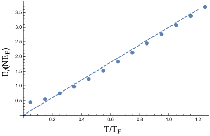
This equation has to be solved numerically. In the high temperature limit $\zeta_{0}=6(T/T_{F})^{3}$. The experiments do not measure $T/T_{F}$, but only the total energy $E/(NE_{F})$. We can compute the energy using the virial theorem. We get

$$\frac{E}{NE_{F}}=\left(\frac{T}{T_{F}}\right)\frac{\int d^{3}x\,x^{2}g\left(\zeta_{0}\exp\left(\frac{x^{2}}{2}\right)\right)}{\int d^{3}x\,g\left(\zeta_{0}\exp\left(\frac{x^{2}}{2}\right)\right)}\,.$$ (31)

In the high temperature limit $E/(NE_{F})=3(T/T_{F})$. We can use equ. (30) and (31) to compute both $T/T_{F}$ and $\zeta$ at the trap center as a function of $E/(NE_{F})$. Note that these relations do not explicitly depend on $N$, but the units of distance, density, and pressure implicitly depend on the number of particles. Figure 7 shows $E/(NE_{F})$ as a function of $T/T_{F}$. We observe that even though the full energy density and pressure differ significantly from that of a free gas, the relation between $E$ and $T$ of a trapped interacting gas is close to that of a trapped free gas, except at very low temperature. As an example we consider the case $E/(NE_{F})=1.49$. We find

$$\left(\frac{T}{T_{F}}\right)_{\it full}=0.538,\hskip 8.5359pt\left(\frac{T}{T_{F}}\right)_{\it free}=0.496,\hskip 8.5359pt\zeta_{0}=1.154.$$ (32)

The corresponding density and pressure profiles are shown in Fig. 8. We compare to the density and pressure of a free Boltzmann and Fermi gas at the same $E/(NE_{F})$.

Figure 8: Initial density $\bar{n}(\bar{x})$ and pressure $\bar{P}(\bar{x})$ of a trapped gas at $E/(NE_{F})=1.49$. The full line shows the result for the MIT equation of state, the dotted line is the Boltzmann limit, and the dashed line is a free Fermi gas. The distance is given in units of $\tilde{\omega}_{x}^{-1}x_{0}$, and the density is in units of the central density of a free Boltzmann gas.

Figure 9: Temperature correction factor $G(x)$. The points and the solid line show the function $G(x)$ computed from the parametrization of $h(\zeta)$ given in the text. The dashed line is the fit in equ. (39).

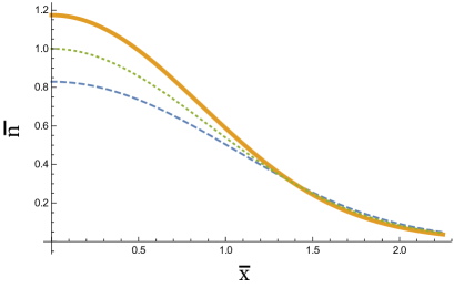
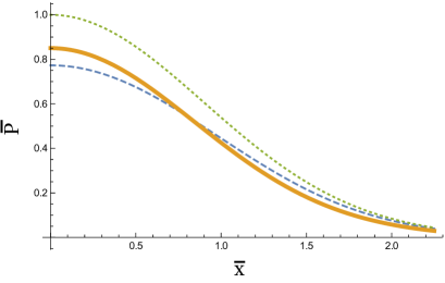
Below we will compare the hydrodynamic evolution initialized with the free Boltzmann gas to that initialized with the correct density and pressure profile of an interacting gas. One complication is that for a free Boltzmann gas the temperature is given by $P/n$, whereas for the full equation of state the temperature is a more complicated function of $P$ and $n$. In particular, for the profiles shown in Fig. 8 the ratio $P/n$ is not spatially constant.

Figure 10: This figure shows the time evolution of the aspect ratio $\sigma_{x}/\sigma_{y}$ (extracted from a Gaussian fit) for $E/(NE_{F})=1.49$. The green dots show a hydrodynamic simulation with Gaussian (free Boltzmann gas) initial conditions, and the red dots are obtained using the initial conditions shown in Fig. 8. The solid line takes into account the exact equation of state in computing the temperature dependence of the shear viscosity. The gray data points are measurements for $E/(NE_{F})=1.49$ from Joseph et al.

In order to determine the temperature we follow the method suggested in Appendix A of Schafer:2010dv . Consider the function

$$F(\zeta)=\frac{2f(\zeta)^{3/2}}{g(\zeta)^{5/2}}.$$ (33)

From equ. (23) and (27) we know that this function is proportional to $P^{3/2}/n^{5/2}$. The fugacity can then be computed using the inverse function $F^{-1}(x)$. We have

$$\zeta=F^{-1}\left(\frac{2}{(2\pi)^{3/2}}\frac{(mP)^{3/2}}{n^{5/2}}\right).$$ (34)

From the fugacity we can compute the temperature

$$T=\frac{g(\zeta)}{f(\zeta)}\,\frac{P}{n}\,.$$ (35)

In dimensionless units, this result can be written as

$$\bar{T}=G(x)\frac{\bar{P}}{\bar{n}}\,,$$ (36)

where we have defined the correction factor

$$G(x)=\frac{g(F^{-1}(x))}{f(F^{-1}(x))}\,,$$ (37)

and the variable

$$x=\frac{16}{9}\left(\frac{3}{2}\frac{T}{T_{F}}\right)^{3/2}\frac{\bar{P}^{3/2}}{\bar{n}^{5/2}}\,.$$ (38)

Here $T/T_{F}$ is the initial temperature of the trap. This quantity enters through the overall normalization of the density. The function $G(x)$ is fixed once $h(\zeta)$ has been determined. However, since the definition of $G(x)$ involves inverse functions it has to be computed numerically. In practice, we have parametrized $G(x)$ in analogy with $h(\zeta)$,

$$G(x)=\frac{1+d_{1}/x+d_{2}/x^{2}}{1+d_{3}/x+d_{4}/x^{2}}\,.$$ (39)

We find

$$d_{1}=1.8052, d_{2}=-0.0022,$$ (40)

$$d_{3}=1.3668, d_{4}=0.1179.$$

The function $G(x)$ together with the fit in equ. (39) is shown in Fig. 9. Note that this parameterization is restricted to the regime $T\mathrel{\hbox to0.0pt{\lower 4.0pt\hbox{\hskip 1.0pt$\sim$}\hss}\raise 1.0pt\hbox{$>$}}T_{c}$.

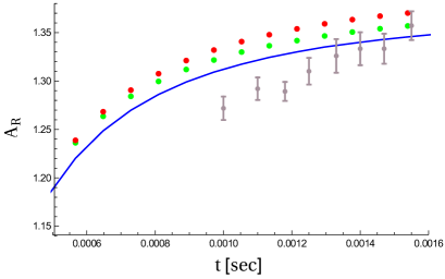
Finally, we can study the effect of the equation of state on the anisotropic expansion. Figure 10 shows the case $E/(NE_{F})=1.49$. The green dots show the aspect ratio computed using initial conditions obtained from the free equation of state, and the red dots show the result for the initial conditions shown in Fig. 8. The red dots are computed using $\eta\sim T^{3/2}$ with $T=P/n$, and the solid line is computed using the full equation of state, including the correction factor $G(x)$. For comparison, we also show a set of aspect ratio measurements from Joseph:2014 . No attempt was made to fit the data by adjusting $\eta_{0}$. We observe that the initial state has a significant effect on the time evolution. This effect is more than compensated by the effect of using the correct temperature $T=T(P,n)$.

References

- (1) J. A. Joseph, E. Elliott, J. E. Thomas, “Shear viscosity of a universal Fermi gas near the superfluid phase transition,” Phys. Rev. Lett. 115, 020401 (2015) [arXiv:1410.4835 [cond-mat.quant-gas]].
- (2) M. J. H. Ku, A. T. Sommer, L. W. Cheuk, and M. W. Zwierlein, “Revealing the Superfluid Lambda Transition in the Universal Thermodynamics of a Unitary Fermi Gas,” Science 335, 563 (2012) [arXiv:1110.3309 [cond-mat.quant-gas]].
- (3) T. Schäfer and D. Teaney, “Nearly Perfect Fluidity: From Cold Atomic Gases to Hot Quark Gluon Plasmas,” Rept. Prog. Phys. 72, 126001 (2009) [arXiv:0904.3107 [hep-ph]].
- (4) A. Adams, L. D. Carr, T. Schäfer, P. Steinberg and J. E. Thomas, “Strongly Correlated Quantum Fluids: Ultracold Quantum Gases, Quantum Chromodynamic Plasmas, and Holographic Duality,” New J. Phys. 14, 115009 (2012) [arXiv:1205.5180 [hep-th]].
- (5) T. Schäfer, “Fluid Dynamics and Viscosity in Strongly Correlated Fluids,” Ann. Rev. Nucl. Part. Sci. 64, 125 (2014) [arXiv:1403.0653 [hep-ph]].
- (6) P. Kovtun, D. T. Son and A. O. Starinets, “Viscosity in strongly interacting quantum field theories from black hole physics,” Phys. Rev. Lett. 94, 111601 (2005) [hep-th/0405231].
- (7) I. Bloch, J. Dalibard, W. Zwerger, “Many-Body Physics with Ultracold Gases” Rev. Mod. Phys. 80, 885 (2008) [arXiv:0704.3011].
- (8) S. Giorgini, L. P. Pitaevskii, S. Stringari, “Theory of ultracold atomic Fermi gases” Rev. Mod. Phys. 80 1215 (2008) [arXiv:0706.3360].
- (9) J. Kinast, A. Turlapov, J. E. Thomas, “Breakdown of Hydrodynamics in the Radial Breathing Mode of a Strongly-Interacting Fermi Gas,” Phys. Rev. A 70, 051401(R) (2004) [arXiv:cond-mat/0408634 [cond-mat.soft]].
- (10) T. Schäfer, “The Shear Viscosity to Entropy Density Ratio of Trapped Fermions in the Unitarity Limit,” Phys. Rev. A 76, 063618 (2007) [arXiv:cond-mat/0701251].
- (11) A. Turlapov, J. Kinast, B. Clancy, L. Luo, J. Joseph, J. E. Thomas, “Is a Gas of Strongly Interacting Atomic Fermions a Nearly Perfect Fluid” J. Low Temp. Phys. 150, 567 (2008) [arXiv:0707.2574].
- (12) G. M. Bruun, H. Smith, “Frequency and damping of the Scissors Mode of a Fermi gas”, Phys. Rev. A 76, 045602 (2007) [arXiv:0709.1617].
- (13) C. Cao, E. Elliott, J. Joseph, H. Wu, J. Petricka, T. Schäfer and J. E. Thomas, “Universal Quantum Viscosity in a Unitary Fermi Gas,” Science 331, 58 (2011) [arXiv:1007.2625 [cond-mat.quant-gas]].
- (14) E. Elliott, J. A. Joseph, J. E. Thomas, “Anomalous minimum in the shear viscosity of a Fermi gas,” Phys. Rev. Lett. 113, 020406 (2014) [arXiv:1311.2049 [cond-mat.quant-gas]].
- (15) E. Elliott, J. A. Joseph, J. E. Thomas, “Observation of conformal symmetry breaking and scale invariance in expanding Fermi gases,” Phys. Rev. Lett. 112, 040405 (2014) [arXiv:1308.3162 [cond-mat.quant-gas]].
- (16) J. Brewer, M. Mendoza, R. E. Young and P. Romatschke, “Lattice Boltzmann simulations of a strongly interacting two-dimensional Fermi gas,” Phys. Rev. A 93, no. 1, 013618 (2016) [arXiv:1507.05975 [cond-mat.quant-gas]].
- (17) K. H. Ackermann et al. [STAR Collaboration], “Elliptic flow in Au + Au collisions at = 130 GeV,” Phys. Rev. Lett. 86, 402 (2001) [nucl-ex/0009011].
- (18) S. S. Adler et al. [PHENIX Collaboration], “Elliptic flow of identified hadrons in Au+Au collisions at = 200-GeV,” Phys. Rev. Lett. 91, 182301 (2003) [nucl-ex/0305013].
- (19) K. Aamodt et al. [ALICE Collaboration], “Elliptic flow of charged particles in Pb-Pb collisions at 2.76 TeV,” Phys. Rev. Lett. 105, 252302 (2010) [arXiv:1011.3914 [nucl-ex]].
- (20) M. Bluhm and T. Schäfer, “Dissipative fluid dynamics for the dilute Fermi gas at unitarity: Anisotropic fluid dynamics,” Phys. Rev. A 92, no. 4, 043602 (2015) [arXiv:1505.00846 [cond-mat.quant-gas]].
- (21) W. Florkowski and R. Ryblewski, “Highly-anisotropic and strongly-dissipative hydrodynamics for early stages of relativistic heavy-ion collisions,” Phys. Rev. C 83, 034907 (2011) [arXiv:1007.0130 [nucl-th]].
- (22) M. Martinez and M. Strickland, “Dissipative Dynamics of Highly Anisotropic Systems,” Nucl. Phys. A 848, 183 (2010) [arXiv:1007.0889 [nucl-th]].
- (23) P. A. Pantel, D. Davesne and M. Urban, “Numerical solution of the Boltzmann equation for trapped Fermi gases with in-medium effects,” Phys. Rev. A 91, 013627 (2015) [arXiv:1412.3641 [cond-mat.quant-gas]].
- (24) M. Bluhm and T. Schäfer, “Model-independent determination of the shear viscosity of a trapped unitary Fermi gas: Application to high temperature data,” Phys. Rev. Lett. 116, no. 11, 115301 (2016) [arXiv:1512.00862 [cond-mat.quant-gas]].
- (25) G. M. Bruun, H. Smith, “Viscosity and thermal relaxation for a resonantly interacting Fermi gas”, Phys. Rev. A 72, 043605 (2005) [cond-mat/0504734].
- (26) T. Schäfer, “Dissipative fluid dynamics for the dilute Fermi gas at unitarity: Free expansion and rotation,” Phys. Rev. A 82, 063629 (2010) [arXiv:1008.3876 [cond-mat.quant-gas]].
- (27) P. Colella, P. R. Woodward, “The Piecewise Parabolic Method (PPM) for Gas-Dynamical Simulations,” J. Comp. Phys. 54, 174 (1984).
- (28) J. M. Blondin, E. A. Lufkin, “The piecewise-parabolic method in curvilinear coordinates,” Astrophys. J. Supp. Ser. 88, 589 (1993).
- (29) T. Enss, R. Haussmann and W. Zwerger, “Viscosity and scale invariance in the unitary Fermi gas,” Annals Phys. 326, 770 (2011) [arXiv:1008.0007 [cond-mat.quant-gas]].
- (30) G. Wlazlowski, P. Magierski, A. Bulgac and K. J. Roche, “The temperature evolution of the shear viscosity in a unitary Fermi gas,” Phys. Rev. A 88, 013639 (2013) [arXiv:1304.2283 [cond-mat.quant-gas]].
- (31) G. Rupak and T. Schäfer, “Shear viscosity of a superfluid Fermi gas in the unitarity limit,” Phys. Rev. A 76, 053607 (2007) [arXiv:0707.1520 [cond-mat.other]].
- (32) W. Zwerger, “Strongly Interacting Fermi Gases,” Proceedings of the International School of Physics ”Enrico Fermi” - Course 191 ”Quantum Matter at Ultralow Temperatures” edited by M. Inguscio, W. Ketterle, S. Stringari and G. Roati (2016), pp. 63-142 [arXiv:1608.00457 [cond-mat.quant-gas]].
- (33) S. Nascimbene, N. Navon, K. Jiang, F. Chevy, C. Salomon, Nature 463, 1057 (2010) [arXiv:0911.0747[cond-mat.quant-gas]].
- (34) P. Romatschke and R. E. Young, “Implications of hydrodynamic fluctuations for the minimum shear viscosity of the dilute Fermi gas at unitarity,” Phys. Rev. A 87, no. 5, 053606 (2013) [arXiv:1209.1604 [cond-mat.quant-gas]].