ELUCID – Exploring the Local Universe with the reConstructed Initial Density field. II: Reconstruction diagnostics, applied to numerical halo catalogs

Abstract

The ELUCID project aims to build a series of realistic cosmological simulations that reproduce the spatial and mass distribution of the galaxies as observed in the Sloan Digital Sky Survey (SDSS). This requires powerful reconstruction techniques to create constrained initial conditions. We test the reconstruction method by applying it to several $N$-body simulations. We use 2 medium resolution simulations from each of which three additional constrained $N$-body simulations were produced. We compare the resulting friend of friend catalogs by using the particle indexes as tracers, and quantify the quality of the reconstruction by varying the main smoothing parameter. The cross identification method we use proves to be efficient, and the results suggest that the most massive reconstructed halos are effectively traced from the same Lagrangian regions in the initial conditions. Preliminary time dependence analysis indicates that high mass end halos converge only at a redshift close to the reconstruction redshift. This suggests that, for earlier snapshots, only collections of progenitors may be effectively cross-identified.

1. Introduction

One of the key aspects of modern cosmology is to interpret the distribution and properties of galaxies in the sky. The diversity of galaxy properties is inherent to their history and environment.

The formation and evolution of galaxies is generally understood within the $\Lambda$CDM paradigm. Matter itself is dominated by a dark component: the Dark Matter subject to gravitational interactions. Galaxies are understood to reside in dark matter halos, that act as a gravitational potential wells. These follow a pattern of hierarchical structure formation, where the smaller structures form first and merge to build larger and larger ones. The gas itself is bound to these structures and as they build up, baryonic processes take place leading to the formation of stars in galaxies that further evolve and interact within those halos.

Structure formation is thus understood as a non-linear process, that cannot be fully described analytically. Building these structures requires the use of specific numerical methods: $N$-body simulations. These codes focus on the Dark Matter component, and successfully describe the formation of structures by implementing gravitational interactions on large scales. Dark Matter is described numerically by data points (otherwise referred as particles) that trace a mass element corresponding to a volume element of the early ’homogeneous’ universe.

Over the decades, such simulations have been widely used, with little variation in term of physics. Combined with ever decreasing limitations of computer resources and vast improvement in term of implementations, larger volumes can be explored with increasing resolution.

Distributions and properties of galaxies are observed with ever increasing accuracy, but little information concerning the dominating component can be inferred. Nevertheless various methods exist to explore the formation of galaxies within Dark Matter halos. The most direct one is to numerically solve the evolution of the baryonic component on top of the Dark Matter one. This method requires more complex implementations than $N$-body simulations, with gas described either as (i) numerical data points with associated density (Smooth Particles hydrodynamics: Springel et al., 2001b; Springel, 2005; Wadsley et al., 2004), (ii) grid cells fixed in the volume (cells are refined and unrefined as required to explore high gas density while neglecting low density regions) (nested grids or Adaptive Mesh Refinement: Kravtsov et al., 1997; Kravtsov, 2003; Teyssier, 2002) (iii) or moving cells (the gas element is associated with a numerical point within a volume defined from the distribution of nearby mesh points through Voronoi tesselation) (Springel, 2010). Less computationally intensive methods involve applying models on the scale of the halo itself where evolution can be traced with merger trees. These Semi-Analytical Models (SAM) have been successfully applied to halo catalogs extracted from $N$-body simulations (White & Frenk, 1991; Kauffmann et al., 1993; Somerville & Primack, 1999; Cole et al., 2000; van den Bosch, 2002; Hatton et al., 2003; Kang et al., 2005; Croton et al., 2006; Baugh, 2006).

Both types of methods are used to create mock galaxy catalogs. These catalogs are usually confronted with the observed ones and have been quite successful in reproducing statistical features; such as the 2 point correlation functions, luminosity functions, color distributions and star formation rates. Both sub-grid models (applied to gas elements) and semi-analytical models (applied to halos) require determination of a large number of parameters which can lead to some degeneracies.

Even more simplified approaches are halo occupation distribution models, where observed galaxies are assigned to halos by matching the halo mass and stellar mass functions (Jing et al., 1998, 2002; Berlind & Weinberg, 2002; Bullock et al., 2002; Scranton, 2002; Yang et al., 2003; van den Bosch et al., 2003; Behroozi et al., 2010; Rodríguez-Puebla et al., 2015). Such methods have been successful in defining the Stellar Mass Halo Mass (SMHM) relation but the scatter of this relation still remains uncertain and difficult to interpret. Higher constraints can be obtained by comparing specific galaxies, their environment and the Inter Galactic Medium (IGM). To achieve this, one needs to obtain one or several simulations that match the distribution of galaxies as seen in the sky. In order to understand how an $N$-body simulation can reproduce a given distribution, one must have a basic understanding of how a cosmological $N$-body code works. Basically the distribution of matter (here dark matter only), is represented by numerical data points (particles) describing the mass and volume element of this matter. Since dark matter answers to gravity alone, the motion of this dark matter element obeys the Poisson equation. A cosmological $N$-body code is essentially just a Poisson solver, with various optimizations rendering the computation possible. An $N$-body simulation starts at early redshift ($\sim 100$) from a uniform distribution of particles following a grid. But the disposition of particles cannot be perfectly uniform in position and velocity since then the distribution would remain unchanged. Obtaining a realistic simulation implies applying small shifts in both positions and velocities on the initial grid nodes. This displacement field corresponds to the Initial Conditions (IC). They are usually randomly generated from the initial power spectrum for a given cosmology. From the same set of ICs any $N$-body code would produce the same density field. However, the formation and evolution of large scale structures is a non-linear process. The only way to derive the matter distribution is thus to run the numerical simulation.

Reconstructing a particular density field with an $N$-body simulation consists in finding, among all possible sets of ICs, the one that would produce the closest match. To achieve this purpose, it is not realistic to create an infinite number of trial sets of ICs, run an $N$-body simulation from each set and chose the optimal one. The solution is to use other numerical techniques to reverse engineer the displacement field (that characterize a set of ICs) from the target density field.

Since the pioneering work of Hoffman & Ribak (1991) and Nusser & Dekel (1992), many methods have been developed to reconstruct ICs of the local universe. These methods use either redshift surveys of galaxies (Heß et al., 2013; Wang et al., 2016) or radial peculiar velocities (Kravtsov et al., 2002; Klypin et al., 2003; Gottloeber et al., 2010; Sorce et al., 2016) of low redshift galaxies as tracers of the cosmic density field at the present day. In order to derive ICs from these low redshift tracers several dynamical models are adopted in the literature; (i) linear theory (Hoffman & Ribak, 1991; Gottloeber et al., 2010), (ii) Lagrangian perturbation theory (Nusser & Dekel, 1992; Brenier et al., 2003; Lavaux, 2010; Jasche & Wandelt, 2013; Kitaura, 2013; Wang et al., 2013; Doumler et al., 2013) or (iii) particle-mesh (PM) dynamics (Wang et al., 2014). These dynamical models can be applied either backwards or forwards in time. Zel’dovich approximation (Zel’dovich, 1970) has been classically used to trace the density field back in time to the linear regime (Nusser & Dekel, 1992; Doumler et al., 2013; Sorce et al., 2014). Recently, several studies (Jasche & Wandelt, 2013; Kitaura, 2013; Wang et al., 2013; Heß et al., 2013; Wang et al., 2014) have implemented forward dynamical models within Markov Chain Monte Carlo algorithms. These bayesian methods gradually adjust the phases and amplitudes of the ICs until the evolved density field closely matches the one traced by the observed galaxy population. We refer to Wang et al. (2014, 2016) for a more detailed discussion on the advantages and shortcomings of the various methods.

The ELUCID project (Exploring the Local Universe with the reConstructed Initial Density field) consists in using the large amount of data gathered by the SDSS (Sloan Digital Sky Survey) to map the local universe and generate reliable simulations reproducing the distribution of large scale structures in that survey. The first large ELUCID simulation was completed in 2015: it corresponds to a WMAP 5^th year cosmology with $\Omega_{M}=0.258$, $\Omega_{\Lambda}=0.742$ and $h=0.72$. The simulation volume is a box of 500 Mpc/h per side, where matter is described by $3072^{3}$ particles corresponding to a mass resolution of $3.1\times 10^{8}$ ${\rm h}^{-1}{\rm M}_{\odot}$. A more detailed background of the ELUCID project is given in Appendix A.

One of the main applications of the ELUCID simulation is to build realistic mock catalogs by applying various SAMs to the reconstruction. The validity of the model can be then tested by direct comparison with the original observed SDSS sample and group catalog derived using the method of Yang et al. (2005, 2007). The first problem is to build a framework for a direct comparison. This means devising a reliable criteria for identifying the most likely reconstruction of a given observed group. The second problem is to differentiate between the effects of the reconstruction method and those of the SAM.

In Wang et al. (2014), a forward method that employs the Hamiltonian Markov Chain Monte Carlo (HMC) algorithm and the PM dynamics was developed. This method was tested with $N$-body simulations in order to find the best set of parameters. The main criteria was the similarity of the respective initial power spectra and of the halo mass functions of an original Dark Matter only simulation and its reconstruction. The simulation sample they used is independent of any baryonic physics and observational bias. For this reason, this simulation data set may be used to prepare the analysis of the ELUCID simulations by exploring the limitations of the reconstruction technique itself.

In this paper, we make use of part of the $N$-body simulations sample from Wang et al. (2014). More specifically we use halo catalogs extracted from these simulations. We first devise a method to match halos in the original simulation to halos in the reconstructed one. This catalog of matched halo pairs can be used to test alternative criteria that can be applied to the ELUCID simulations . Additionally various internal properties of halos, such as shape, orientation or angular momentum can be compared. More precisely, given a reconstructed halo, we would be able to identify which of its properties were most likely to be constrained by the reconstruction. Furthermore, $N$-body simulations contain the full formation history of the halos they describe. By applying this cross-identification of halos in the original and reconstructed simulations at different times, one can assess how much of the formation history has been reproduced by the reconstruction method. Since both internal properties and formation histories of halos can have a strong impact on the SAM, these questions are extremely relevant to the ELUCID project.

We detail the method used in the paper in section 2, before focusing on the results in section 3. We discuss our results after a short summary in section 4.

2. Method

In §2.1, we introduce the $N$-body simulation sample and explain how it was processed to obtain the halo catalogs. We describe in detail in §2.2, the halo cross-comparison method.

2.1. Simulations

Figure 1.— This diagram introduces how a pair of original/reconstructed simulations were generated. We start from initial conductions randomly generated from the initial power spectrum. The original $N$-body simulation is produced from these initial conditions down to redshift 0. The last output is processed as to produce a new set of initial conditions. This new set is used to run the reconstructed $N$-body simulation.

We summarize in Figure 1 the processes involved in creating a simulation pair. The first one (referred as the original) is built from random initial conditions (generated from the power spectrum predicted for the cosmology), the second simulation is a reconstruction of the first. The initial conditions of the reconstructed simulation are generated following Wang et al. (2014). As the schematic shows, we proceeded as follows:

1. The original simulation is run from random initial conditions.

2. The final (redshift 0) output is post-processed with a gaussian smoothing kernel to produce the density field.

3. This density map is used as input for the reconstruction method to produce a reconstruction of the initial conditions.

4. The reconstructed simulation is run from the reconstructed initial conditions.

We list in Table 1, the simulation data set used in this paper. Each simulation has $512^{3}$ particles, of mass $2\times 10^{10}$ ${\rm M}_{\odot}$, in a comoving box of side 300 ${\rm h}^{-1}{\rm Mpc}$. The cosmological parameters are $\Omega_{M}=0.258$, $\Omega_{\Lambda}=0.742$ and $h=0.72$. The cosmology is not relevant, as we focus rather on numerical techniques than on the effect of the cosmological model. We emphasize, that all simulations are run with the same $N$-body code, here GADGET2 (Springel, 2005), with the same time outputs (60 outputs equally spaced in $\Delta\log(1/1+z)$ from $z=18$ to $z=0$). The only difference between simulations mentioned in this paper is in the initial conditions.

Name	$\sigma_{\rm HMC}$ [Mpc/h]	$\sigma_{\rm PM}$ [Mpc/h]	NPM
L300A
L300Ac1	2.25	1.5	10
L300Ac2	3	1.5	10
L300Ac3	4.5	1.5	10
L300B
L300Bc1	2.25	1.5	10
L300Bc2	3	1.5	10
L300Bc3	4.5	1.5	10

Table 1List of $N$-body simulations. We have two series of simulations L300A and L300B. The original simulations are L300A and L300B. From each of the original simulations, 3 reconstructions where performed. The extensions c1, c2 and c3 is used to distinguish them from their respective original and refer to the corresponding sets of reconstruction parameters ($\sigma_{\rm HMC}$, $\sigma_{\rm PM}$, N_PM) indicated in the row.

As indicated in Table 1, we have 2 independent $N$-body simulations: L300A and L300B. For each of these original simulations 3 sets of reconstructed simulations were generated. The reconstruction method is detailed in Wang et al. (2014). It depends on the density smoothing $\sigma_{\rm HMC}$ and the Particle Mesh (PM) parameters: N_PM (number of steps) and $\sigma_{\rm PM}$ (grid length). The smoothing scale had to be chosen to reduce the resolution effects of the PM model. Choosing $\sigma_{\rm HMC}\leq\sigma_{\rm PM}$ leads to significant discrepancies in the 2 point correlation functions at small scales (see Figure 3 Wang et al., 2014). The smallest $\sigma_{\rm HMC}$ we consider is $1.5\times\sigma_{\rm PM}$, while $2\times\sigma_{\rm PM}$ renders these discrepancies negligible. The choice of $3\times\sigma_{\rm PM}$ represents a compromise between further reducing this resolution effect and limiting the loss of information at small scales. In this paper we use the simulation sample that is used to explore the impact of the density smoothing with fixed PM parameters. We rather focus halo catalogs extracted from these simulations than the raw simulations data.

There are a large variety of group-finding algorithms, starting from simple halo finding methods such as the friend of friend (Davis et al., 1985, FOF) or Spherical Over-Density (Lacey & Cole, 1994, SOD), through more elaborate subhalo finders such as SUBFIND (Springel et al., 2001a), AdaptaHOP (Aubert et al., 2004; Tweed et al., 2009), or AHF (Knollmann & Knebe, 2009) to even more complex ones such as phase-space group-finders 6DFOF (Diemand et al., 2006), HST (Maciejewski et al., 2009), or RockStar (Behroozi et al., 2013) (see review by Knebe et al., 2011; Onions et al., 2012, and subsequent “subhalos going notts” papers). Aside from the algorithm used to collect particles, the properties associated with the halos are not necessarily standardized. The position can be defined as the center of mass of the collection of particles, the position of the density peak or the position of the most bound particle. As mentioned by Cui et al. (2016), the two positions are normally aligned with each other. The mass itself can be defined as the total mass of the collection of particles, or as the virial mass defined as the total mass within a spherical (or ellipsoidal) region. This virial region can be defined as an over-density of either 200$\times\overline{\rho_{\rm DM}}$, 200$\times\overline{\rho_{\rm crit}}$ or $\Delta(z)\times\overline{\rho_{\rm crit}}$. These criteria also lead to multiple definitions of halo size, boundary and shape.

For simplicity, we have used the standard friend of friend (FOF Davis et al., 1985) algorithm where groups are built by iteratively linking particles to all its neighboring particles closer than a specific distance. In our case, the distance used is $0.2\times\overline{\Delta}_{N}$ ($b=0.2$) where $\Delta_{N}=L_{\rm box}/{N^{1/3}}$ is the mean inter-particular distance of the $N$-body simulation in a volume of side $L_{\rm box}$ ($N^{-1/3}$ in box units). We also mention that no unbinding procedure have been applied to the halo catalogs. This group-finder is often the baseline for more complex ones. If we were not to find any match between FOF halo catalogs, it is unlikely we would find any between catalogs build using other group-finders. Internal properties comparison and subhalo cross-identification can still be implemented at a later stage for FOF cross-identified halos.

Our starting point here for each simulation is a list of particles with their associated indexes, positions, velocities and mass. We also have a list of halos defined as a collection of particle indexes. From this collection we can easily calculate the position, mass or other useful quantities relevant to the halo.

2.2. Halo cross-identification

Having introduced the data we use in this paper, we now describe the comparison algorithm.

2.2.1 General idea

Figure 2 illustrates the initial layout of a halo cross identification method applied to two catalogs A and B.

1. We compare halo catalog B to halo catalog A:

   • Each halo in catalog B can be associated to at most one halo in catalog A. Multiple halos B₁, B₂… can be associated to the same halo A_i in catalog A (upper half of Figure 2a).

   • Only one of these halos (B₁, B₂…) can be “cross-identified” with A_i, the others remain “associated” with A_i (upper half of Figure 2b).

2. We compare halo catalog A to halo catalog B, following the same method to ensure consistency (lower halves of Figures 2a and 2b).

There are multiple reasons for us to design the method so that the comparison is run in both directions. The first reason is not to introduce any bias to our interpretation by implementing a fiducial. Let’s suppose that for each halo A, the best match found in B is systematically larger. We cannot rule out that this systematic is not caused by the matching criteria unless we reverse the problem. Running the comparison both ways, provides the means to ensure that the cross-identification is consistent. The second reason is the interpretation of the non cross-identified halos. To illustrate this, we now suppose that catalog A is a subset of catalog B. By comparing catalog B to catalog A, we would find that every halo in B is cross-identified. We would then conclude that catalog A and B are identical. But by comparing catalog A to catalog B, we would find a population of halos in catalog B that are not cross-identified. We would draw the correct conclusion; catalog A and B are different.

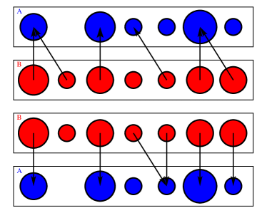
(a) We search for possible matches (single-tip arrows) of halos B in catalog A (top) and for possible matches of halos A in catalog B (bottom). This constitutes a mapping of all associations.

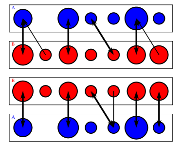
(b) Top: Among possible matches of halos A in catalog B one is selected as cross-identification (double-tip arrows), the remaining associations are still indicated. Bottom: the same selections is applied for matches of halos B in catalog A.

Figure 2.— Illustration of the cross-identification method, the method is applied twice from catalog B to catalog A and from catalog A to catalog B.

As detailed in Figure 2, a one way identification can provide multiple correspondences for a halo. If we only care about cross-identification (double tip arrow), we could choose one possibility and discard the others. We chose however to keep track of these discarded choices as associated halos (single tip arrow) and distinguish them from halos that have no possible counterparts. In order to collect these associated halo populations from both catalogs, it is also necessary to run the comparison both ways.

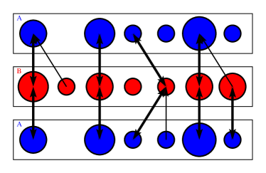
Figure 3.— Code optimization: The layout of the algorithm is reorganized, lower part of inverted and combined to the top one. The same cross-identification search can be implemented in both directions as one run.

As we have described it, our algorithm need to be run twice, once from B to A and once from A to B. The results have then to be compared for possible mismatches. One very simple improvement, is that instead of reading/using both catalogs twice, the code can be restructured to read/use only one of the catalogs twice and the other once. The procedure described in Figure 2 becomes that illustrated in Figure 3. We note here that we used a A-B-A configuration, but a B-A-B configuration would provide the same answers. The structure of the cross-comparison between catalogs takes the form of a tree, with one main branch (trunk) for cross-identification and at secondary branches for associations.

2.2.2 Cross-identification criteria

Since the aim of reconstruction is to obtain the same spatial distribution of large scale structures, the most logical choice would be to compare the position of halos. Minimizing the distance may mislead the algorithm into pairing up halos of very different masses, while the correct reconstructed halo could be found at a slightly larger distance. If one wanted to focus on the most massive structures only, one could simply, cross-identify halos starting from the high mass end of the mass function. But this cheap and easy method would quickly break down after a few 100 groups. Solving the problem requires to find a criteria that would minimize both differences in positions and mass between original and reconstructed halos matches. Wang et al. (2016) implemented such a method to associate galaxy groups to halos in the ELUCID reconstructed simulation. A future cross-comparison method between real and reconstructed data will implement similar criteria within the framework we propose in this paper. The purpose of this paper is to build reliable cross-identified catalogs in order to evaluate and calibrate such a method.

The reason why we use reconstructions of $N$-body simulations is that halos properties are no longer restricted to position, mass and size. Furthermore halo cross-identification is a known problem for simulations. Building a merger-tree consists in associating halos between time outputs. Testing a new group-finder also requires to be cross-compared with a halo catalog built using an other algorithm. In both case, cross-identification is applied for one simulation (e.g. one set of initial conditions) and particles indexes are used as tracers. The problem is solved by optimizing the quantity of particles in common matched halos. But having different initial conditions implies that identical particle indexes have different displacement fields applied to them. Technically, particle indexing has no effect on the simulation outcome, and should be entirely random.

However, in $N$-body simulations, particle indexing is not random. Indexes are assigned following a fixed grid to which the displacement field characterizing the initial conditions is applied. Thinking back to the problem at hand, one may suppose that if the reconstruction proves to be truly efficient, reconstructed halos would appear out of similar regions in the initial conditions. Provided that the same particles indexes are associated to the same coordinates in the initial conditions, we could expect that a perfectly reconstructed halo would have the same particle indexes as the original one. In the case of $N$-body simulations, this means we can apply a tree-builder to the problem.

We can illustrate this by supposing that catalog B is the earlier output. For each halo in catalog B we first map out a list of all possible descendants in catalog A. Each candidate in A has at least one particle in common with halo B, so their common mass is $M_{A\cap B}>0$. This constitutes a graph. To create a merger-tree out of the graph, one need to select one single descendant, and update the list of their progenitors accordingly. In tree-builders, the strength of connections between progenitors and descendent is weighted by a merit function. The most widely used is the normalized shared merit function, and for two halos of masses $M_{A}$ and $M_{B}$ is defined as:

$$\mathcal{M}_{m}(A,B)=\frac{M_{A\cap B}^{2}}{M_{A}\times M_{B}}\,.$$ (1)

For each halo in catalog B, the descendant in catalog A with the highest merit is selected. Among the progenitors found in catalog B, the main progenitor of any halo in catalog A is the one with the highest merit. Going back to the cross-identification problem, cross-identified would be translated as main progenitor and associated as secondary progenitor.

As the review by Srisawat et al. (2013) shows, many tree-builders are available and most are variations of the algorithm by Lacey & Cole (1994). They differ in the way some very technical corrections are implemented. Avila et al. (2014) demonstrate that the choice of group-finder will have a stronger impact on the merger-tree themselves than the choice of tree-builder. The tree-builder used here is TreeMaker (Hatton et al., 2003; Tweed et al., 2009). Using this tree-builder simply requires that the original (as A) and reconstructed (as B) halo catalogs are used as indicated in Figure 3.

This tree-structure is useful for validating the cross-identification. The main branch should start and end with the same halo and secondary branches should contain at most one halo. As one can see from our illustration Figure 3 (or even Figure 2b), this is not necessarily the case. These inconsistencies could represent a problem. In Appendix B, we describe how these inconsistencies are solved before constructing the cross-identified and associated catalogs. Some additional selection is applied for these catalogs. By default we apply a merit threshold of 0.25, but we may increase or decrease this parameter to derive more or less complete or strictly accurate cross-identified catalogs. We chose this value since it can be interpreted as a minimum quadratic average of 50% common mass between two cross-identified groups. For improving the interpretability of the associated catalogs, we systematically use, after cross-identification, a threshold of 50% of the common mass ($M_{A\cap B}/M_{A}>0.5$ for the associated catalog A, $M_{A\cap B}/M_{B}>0.5$ for the associated catalog B). Even though their merit is below the first threshold, discarded cross-identified halos can be added to the associated catalog if their common mass above that second threshold.

3. Results

We assess in §3.1 the effect of the density smoothing scale on the reconstruction. We further test in §3.2 the compatibility of the mass based merit we use to a distance based merit function. The impact of the the merit threshold selection on the cross-identified sample is tested in §3.3. The evolution of the quality of the reconstruction at earlier redshift is explored in §3.4. We check in §3.5, whether earlier time steps of the reconstructed simulations could correspond to more accurate reconstructions.

3.1. Density smoothing and high mass bias

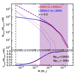
(a) $\sigma_{\rm HMC}=2.25$

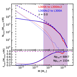
(b) $\sigma_{\rm HMC}=3$

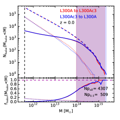
(c) $\sigma_{\rm HMC}=4.5$

Figure 4.— Each subfigure assesses the performances of a different reconstruction of the same original simulation. Top panels: For both original (in red) and reconstruction (in blue) we show the cumulative mass functions of all halos (dashed curves), of the cross-identified subsamples (solid curves) and the associated samples (dotted curves). Bottom panels The last four curves are shown again after normalization by the cumulative mass functions indicated by the horizontal purple dashed line. Np_all denotes the total number of cross-identified pairs, and Np_0.5 the number of pairs for which the reconstruction is 50% complete. In both panels, additional shaded regions indicate the 50% completeness regions, and the vertical dashed line the minimal halo mass.

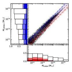
(a) $\sigma_{\rm HMC}=2.25$

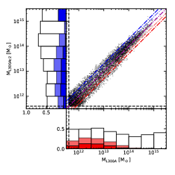
(b) $\sigma_{\rm HMC}=3$

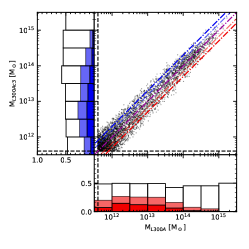
(c) $\sigma_{\rm HMC}=4.5$

Figure 5.— Each subfigure assesses the performances of a different reconstruction of the same original simulation. The scatter plot represents for each cross-identified halo pair, the mass in the reconstructed simulation (ordinate) as a function of the mass in the original simulation. The 1:1 relation is marked as a purple dot-dashed diagonal line. The fraction of data points above and below this line are represented as a function of the medium mass as black histograms respectively on the left panel (over-estimation in the reconstruction) and the bottom panel (over-estimation in the original) respectively. Additional dot-dashed diagonals represents different mass ratios between reconstruction and original, from top left to bottom right: 2 (blue), 1.5 (light blue), 1/1.5 (light red) and 1/2 (red). The fractions above the blue lines (large overestimations in the reconstruction) and below the red ones (large overestimations in the original) are also represented in the horizontal (left) and vertical (bottom) histograms respectively following the same color code. In all panels vertical and horizontals black dashed lines represent the halo mass resolution.

Figure 4 illustrates the effect of the HMC smoothing length on the reconstructed mass function at the final redshift. Each subfigure corresponds to a different value of $\sigma_{\rm HMC}$ used for the reconstruction of the same original simulation. In the top panels, the cumulative mass functions of each catalog are represented as dashed curves. In each case, the mass functions of the reconstruction (in blue) appear quite similar to the original (in red). Using solid curves following the same color code, we also show the cumulative mass functions of the cross-identified subsample of each simulation. At the high mass end, these curves are superimposed on the dashed ones. In figures 4a and 4b, where lower values of $\sigma_{\rm HMC}$ are tested, the reconstructed mass function is higher than in the original.

This mass bias could be caused by an over-production of massive halos in the reconstruction or by a tendency towards reconstructing halos with a larger mass. The former possibility is ruled out since the cross-identified mass function overlaps the mass function of the complete catalog. The lower panel further confirms this statement: it displays (as solid curves) the ratios of the cross-identified mass functions to the mass functions of their respective simulations. We refer to these curves as cross-identified fractions. A systematic over-production of massive halo in the reconstruction would translate at the high mass end as a cross-identified fraction lower than unity for the reconstruction (blue curve), and a cross-identified fraction close to unity for the original (red curve).

These panels also illustrate how the reconstruction degrades as we explore lower masses. Below $10^{14}$ ${\rm h}^{-1}{\rm M}_{\odot}$, the cross-identified sample diverges from the complete one, effectively illustrating the increasing lack of completeness of the reconstruction as we consider lower and lower masses. The cumulative mass functions of associated halos (associated fractions for short) is represented as dotted curves (red for the original, blue for the reconstructions). These associated halo mass functions highlight an additional discrepancy between original and reconstructed simulations. For low $\sigma_{\rm HMC}$ values, associated mass functions appear to be higher for the original especially in the $[10^{12},10^{14}]$ mass range. Associated halos from the original simulation that appear in excess may be found within larger halos in the reconstruction. This trend is likely to be related to the mass excess in reconstructed halos at the high mass end.

In order to further quantify the quality of the reconstruction, we have added some extra information to these figures. We indicate the total number of pairs in the cross-identified sample Np_all. Using both cross-identified fractions, we have estimated the mass from which 50 % of the halo catalog is reconstructed. We start by selecting halos pairs corresponding to cross-identified fractions greater than 0.5 in both simulations. We denote the number of such pairs as Np_0.5. The respective mass range covered by this 50% complete cross-identified sample is represented with shaded regions color coded accordingly to the simulation with the overlap appearing in purple. As we explore larger smoothing lengths from Figures 4a to 4c, the total number of cross-identified pairs Np_all decreases from $\sim 10^{4}$ to $\sim 7000$ then $\sim 4300$ for smoothing lengths 2.25, 3 and 4.5 Mpc/h. The corresponding numbers at 50% completeness are obviously also lower ($\sim 3000$, $\sim 1500$ and $\sim 500$), and are related to smaller mass ranges as the minimum increases ($2\times 10^{13}$, $4\times 10^{13}$ and $9\times 10^{13}$ ${\rm M}_{\odot}$). Additionally the 50% completeness mass range found for the reconstructed simulation appears to be wider in all three cases. This seems to be related to higher values of the mass function for the reconstruction in the high mass end.

It appears from this figure that there is a bias towards increasing halo mass during reconstruction at the high mass end at least. We explore this mass increase further in Figure 5. In order to compare directly the masses of cross-identified halos we have produced a scatter plot. Each point corresponds to a cross-identified pair, with the mass as measured in the reconstructed simulation displayed as a function of the mass as measured in the original one. In order to guide the eye, various mass ratios are indicated with dash-dotted diagonal lines, with the 1:1 relation in purple, 50% and 100% excess for the reconstructed simulation in blue, 50% and 100% excess for the original one in red. The horizontal histograms in the left panel show, as a function of the median mass, the fraction of reconstructed halos with an excess in mass. Excesses greater than 50% and 100% appear in light blue and dark blue. The vertical histograms in the bottom panel show, as a function of the median mass, the fraction of original halos with an excess in mass. Excesses greater than 50% and 100% appear in light red and dark red.

Since the mass bias is most prominent for the smallest smoothing length, it should also appear in Figure 5a. One can assess qualitatively from the scatter plot that there does not seem to be any mass bias in this first case up to $10^{13}$ ${\rm h}^{-1}{\rm M}_{\odot}$. However the bias becomes quite apparent above $10^{13}$ with higher mass found in the reconstruction. The histograms make the high mass bias clearly apparent in Figure 5a, with 90% pairs in the higher mass bins being found with a higher mass in the reconstruction, and 20 % with twice the mass in the reconstruction. As we explore higher HMC smoothing lengths with Figures 5b and 5c, the distributions of points appear centered closer to the equal mass diagonal represented in purple. This is confirmed by the black histograms and the probability of finding mass excess of 50% and 100% appear similar in both the original and the reconstructed simulations.

As Wang et al. (2014) suggest, for a structure formation model that is valid on a scale larger than $\sigma_{\rm HMC}$, the HMC method will introduce non-Gaussian perturbations (non-Gaussianities) into the reconstructed initial conditions. These non-Gaussian initial conditions eventually lead to such an excess in halo masses. As we further confirm here, increasing the smoothing length significantly reduces the mass bias. However it reduces the mass range within which halos are efficiently reconstructed. But we only consider a reconstruction model with $\sigma_{\rm PM}=1.5$ Mpc/h and N${}_{\rm PM}=10$. As mentioned in Wang et al. (2014), to avoid the mass bias the smoothing scale should be of the order of 3 PM cells. In order to improve the mass range with smaller $\sigma_{\rm HMC}$ smoothing, the $\sigma_{\rm PM}$ parameter must be decreased at the cost of increasing the number of steps N_PM. This was demonstrated by Wang et al. (2014), with more accurate reconstructions using N${}_{\rm PM}=40$ and $\sigma_{\rm PM}=0.75$ Mpc/h and $\sigma_{\rm HMC}=2.25$ Mpc/h. Such reconstruction models (with low $\sigma_{\rm PM}$ and high N_PM) are more computationally expensive. They are well suited to produce a single set of reconstructed initial conditions. Less accurate reconstruction models such as the one used here are better adapted for exploration and testing.

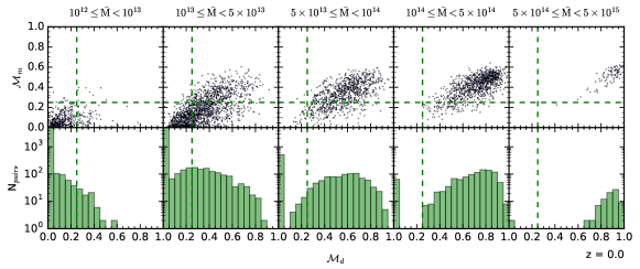
(a) $\sigma_{\rm HMC}=2.25$

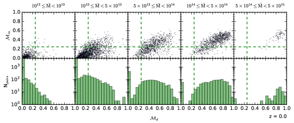
(b) $\sigma_{\rm HMC}=3$

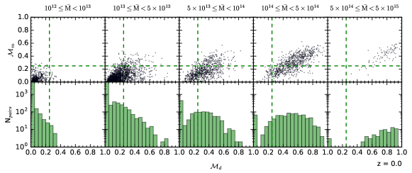
(c) $\sigma_{\rm HMC}=4.55$

Figure 6.— Each subfigure assesses the performances of one of the reconstruction of the same original simulation. For each halo pair cross-identified using our mass based criteria (Eq. 1) we estimate a distance based merit (abscissa, Eq. 2). The top panels show the scatter of the former as a function of the latter. The bottom panels display the number distribution of the cross-identified pairs as a function of the distance based merit. Each column corresponds to a different mass range for median halo mass. As a guide we indicate as dashed green line merit thresholds of 0.25.

3.2. Testing alternative merit functions

So far we have implemented a simple merit function as a criteria for cross-identification. We know that our implementation depends solely on tracing mass from the initial matter distribution. However, the objective of the ELUCID project is to reconstruct halos at the same positions. In order to quantify how close cross-identified halos are, we define this additional distance based merit function:

$$\mathcal{M}_{d}(A,B)=\left(\frac{r_{\rm FOF,A}+r_{\rm FOF,B}}{\left(r_{\rm FOF,A}+r_{\rm FOF,B}\right)+\left|\vec{p_{A}}-\vec{p_{B}}\right|}\right)^{2}\,,$$ (2)

where $\vec{p_{A}}$ and $\vec{p_{B}}$ are the positions of cross identified halos A and B and $r_{\rm FOF,A}$ and $r_{\rm FOF,B}$ their radii. We note that for simplicity, halo positions are defined by their center of mass. Their size $r_{\rm FOF}$ is estimated by the maximum distance of their particle to the center. Effectively, the halos are described as the smallest sphere containing all their particles. One can also note that, for measuring the distance between halos $\left|\vec{p_{A}}-\vec{p_{B}}\right|$, one needs to take periodic boundary conditions into account. The distance criteria we obtain with Eq. 2, is fairly simple, the value goes down to 0 as halos are further from one another and rises to 1 if they are closer. If the halos overlap, $\left|\vec{p_{A}}-\vec{p_{B}}\right|<r_{\rm FOF,A}+r_{\rm FOF,B}+\left|\vec{p_{A}}-\vec{p_{B}}\right|$, then the result of this merit function is larger than 0.25.

We compare directly in Figure 6 (top panels) the two merit functions for different mass bins (using the median mass of the cross-identified pairs). The cross-identified catalog used to create this figure differs from those used in Figures 4 and 5. We have not used any merit threshold, in order to obtain the equivalent distance based merit for unlikely cross-identified pairs. The vertical and horizontal dashed lines display the value of our fiducial merit threshold of 0.25. The bottom panels display the distributions of pairs as a function of the distance based merit. We explore in Figures 6a to 6c the different reconstructions of simulation L300A. For all reconstructions, we clearly see in the top panels, that low mass cross-identified halos do not appear to be close in the simulation volume and typically have low values in the corresponding mass derived merit function. For reconstruction, as we look at increasing mass bins, a new population with distance based merit larger than 0.25 emerges. This bi-modality is made even clearer as we focus on the bottom panels which reveals the number distributions of cross-identified pairs as a function of distance based merit.

These figures show that high mass halos tends to be reproduced with high mass based merits. And as we explore those higher masses, these pairs tend to be quantified with high distance based merits. The two merits functions are strongly correlated for halos pairs that have been most probably correctly cross-identified, especially above $5\times 10^{13}$–$10^{14}$ ${\rm M}_{\odot}$.

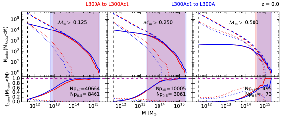
(a) $\sigma_{\rm HMC}=2.25$

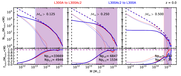
(b) $\sigma_{\rm HMC}=3$

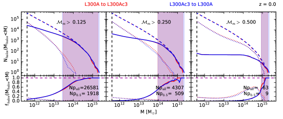
(c) $\sigma_{\rm HMC}=4.55$

Figure 7.— Each subfigure assesses the performances of one of the reconstruction of the same original simulation. Each column contains panels similar to Figures 4a to 4c. For each subfigure, each column correspond to a different selection threshold applied on the merit. Increasing the merit cut reduce the amount of halos pairs in the cross-identified catalog as well as mass range for which the reconstruction can be considered 50% complete.

For any of the smoothing length, we find that these figure are very useful for merit function calibration. For the distance based merit function, the value of 0.25 corresponds to overlap. It is represented by the vertical green dashed line. For our fiducial merit (mass based) function, we find a very low number of non-overlapping cross-identified pairs above our fiducial 0.25 threshold (horizontal green dashed line) . This result shows that we can indeed apply this mass based cross-identification approach to such simulation reconstruction problems.

We can now decide to use our fiducial mass based merit function as a baseline. We suppose that we wish to reproduce the predictions from the mass based merit using the distance based merit. The green dashed lines divide the top panels into 4 domains. We find the true negatives and true positives in the lower left and upper right corners respectively. In the upper left and lower right, we find the false negatives and false positives respectively. We can see that the number of false negatives is very low compared to the number of false positives. This suggests that the performances of the distance based cross-identification may be improved by using a larger merit threshold.

We have explored an existing cross-identified sample to test a potential distance based merit function. The data we used here maximize the value of the mass based one. The distance based merits shown here are over-estimated compared to what would be found by a cross-identification algorithm using this criteria. One must keep in mind that this merit function cannot be fully tested unless implemented in a cross-identification algorithm.

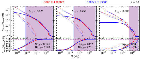
(a) $\sigma_{\rm HMC}=2.25$

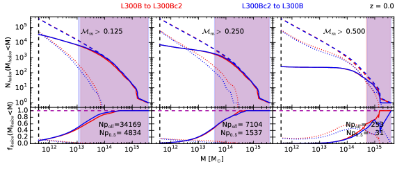
(b) $\sigma_{\rm HMC}=3$

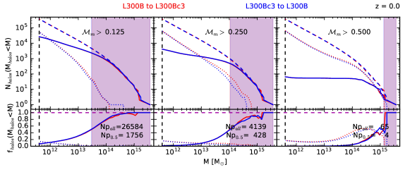
(c) $\sigma_{\rm HMC}=4.55$

Figure 8.— Same as Figure 7 with the L300B simulation and its reconstructions. Results are qualitatively the same but we find a strong variation (up to 25 %) in terms of number of cross-identified pairs for similar sets.

3.3. Applying different merit thresholds

In Figure 7, we explored the cumulative mass functions after cross-identification with multiple merit thresholds, for the different reconstructions as subfigures 7a to 7c. The columns correspond to different values of the merit threshold, increasing from left to right. Our fiducial value of 0.25 used in the previous Figures 4a to 4c are displayed in the central panel.

We note that this selection threshold described and implemented here is not a parameter of the cross-identification method described in §2.2, but is applied a posteriori to generate cross identified and associated catalogs. Each member of any halo pair that does not meet the merit threshold is added to the associated catalog provided that 50% of their mass is found in the other member.

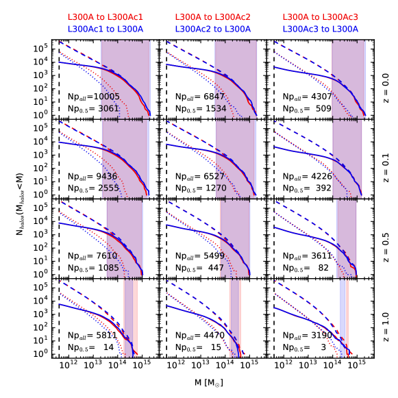
Figure 9.— Similarly to the upper panels of Figures 4a to 4c, we assess the reconstructions through the cumulative mass functions. Each column corresponds to a different reconstruction of the same original simulation, each row correspond to a different redshifts. As we explore larger redshift the reconstruction is degraded both in term of number of cross-identified pairs but also in term of the 50% completeness mass range.

As expected, reducing the value of the merit threshold increases the number of halos to be considered cross-identified. Compared to our fiducial value, dividing this selection threshold by 2, increases the number of halos in the cross-identified catalog by a factor 4 to 6 depending on the reconstruction (HMC smoothing). We have obtained 27000 to 34000 paired halos with this lower threshold, instead of 4000 to 8000 pairs with the fiducial value of 0.25. Allowing for a smaller merit strongly increases the size of the subsample that can be used for cross-comparison. The downside is that a lower value in terms of selection would allow for a much larger mass difference between cross-identified halos. Moreover as Figure 6 suggests, halo pairs with low merits may also be located at larger distances within the simulation box. As we double the value of our fiducial selection threshold, the size of the cross-identified sample is greatly reduced, by a factor of 30 for the smallest smoothing length to a factor of 65 for the largest one. Despite its small size, this catalog should have the advantage of showing halo pairs of very similar masses at close coordinates.

The 50 % completeness region is also strongly affected, with its lower limit moving toward the high mass end (upper limit) with increasing merit threshold. The mass range discrepancy is also more apparent as we consider lower merit thresholds. The merit is thus a very effective criteria to create either a small but accurate reconstructed subsample or a very large but much less accurate one. The former may be preferred for very detailed analysis of specific halos while the latter could be more relevant for large number statistics.

Within the framework of comparing reconstructed simulations, our fiducial value seems to be a good compromise. The size of cross-identified catalog is still dependent on the realization itself. As we go through the same exercise with the second set of simulations L300B in Figure 8. For the smallest value of $\sigma_{\rm HMC}$, we found 15 to 25 % less cross-identified pairs than in the L300A simulation set. There is also a 10% discrepancy in the opposite direction for the medium value of $\sigma_{\rm HMC}$. The difference is less apparent for the largest smoothing, unless we focus on the 50% completeness region where we find larger numbers in the L300A simulation set. This remark highlights the fact that for a specific set of parameters used in the reconstruction the number of reconstructed halos may differ to some potentially large extent. However one aspect of the reconstruction which does not seem to be affected is the 50% completeness mass range. This suggests that the mass range for which we obtain a certain level of completeness is a better indicator for testing a new set of reconstruction parameters.

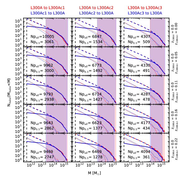
Figure 10.— This figure is similar to Figure 9. Instead of exploring earlier redshifts, we compare earlier snapshots of the reconstruction to the final output of the original simulation. Even though earlier reconstructed mass functions are a better match to the final original mass functions, the cross-identified catalogs contain less pairs, and the 50% completeness mass range gets smaller with increasing time difference.

3.4. Cross-comparison at earlier redshifts

So far, we have shown that the z=0 output is efficiently reconstructed at the higher end of the mass function. This result is obviously by design since reconstruction constraints come from the z=0 smoothed density map. Given that the larger structures should also be present in the simulation, we proceed to compare earlier snapshots to find out whether, by construction, we obtain some constraints at earlier times.

The most logical step to begin with is to directly compare the mass functions for earlier redshifts. In Figure 9, we run the same test as in §3.1 but at multiple redshifts. Each column corresponds to a different reconstruction of the same original simulation, with a different smoothing scale $\sigma_{\rm HMC}$ applied to the density map. Each row corresponds to the different redshifts 0., 0.1, 0.5 and 1 respectively from top to bottom. As in Figures 4a to 4c, we display the number of cross-identified halo pairs (with merit above 0.25) and the mass range corresponding to 50% completeness, the corresponding numbers are also displayed.

Independently of the smoothing length used, one can see in this figure how the reconstruction gets degraded as we explore larger redshifts. The minimum mass from which half the halos should be reconstructed is higher at larger redshift. Notably the number of halos reconstructed above that mass gets smaller as well. If the growth of halos was purely linear, we would expect the high mass end to be populated by the same halos taken at different times and the 50 % completeness mass range would simply shift to the left.

Cross-identified halos at redshift 0 most certainly have multiple progenitors at earlier times. Their main progenitors may also be cross-identified but their secondary progenitors are much less likely to be constrained by the reconstruction technique. The contribution of these secondary progenitors to the mass function with the degradation of the cross-identification of the main progenitor explain why the minimum of the shaded region increases. The cross-identification gets so degraded by redshift 1 that the most massive halos are no longer cross-identified. It is especially evident for the largest smoothing lengths as the 50 % completeness regions no longer overlap.

This degradation can be understood as variation of the merger histories of specific halos. For example, we could imagine a perfectly cross identified pair. They have the same particles, translating to a merit of 1. As we explore earlier time outputs, we can imagine that the original halo is split in two parts, the reconstructed halo being unchanged. The larger part would still be cross-identified but with a lower merit, the smaller part would be associated. At an even earlier time output, it is the reconstructed halo that is split. But a different subset of particles could be removed (the split fraction could be identical). The merit of the cross-identified pair would once again be lowered and an additional associated halo found in the reconstruction. As we imagine that each split is a new progenitor, we understand how individual progenitors (including the main) may no longer be cross-identified. However, the collection of progenitors of the original halo could be cross-identified with the collection of progenitors of the reconstructed one.

3.5. Cross-comparison across redshifts

We pointed out in §3.1, that in the high mass end of the mass function, we find more massive halos in the reconstructed simulation. The issue may be related to an over-merging process, with nearby original halos being reconstructed as one. The halos may thus appear more evolved than in the original simulation. We investigate this possibility in Figure 10. It is similar to Figure 9 with one key difference, the redshift of the original simulation remains fixed (z=0), but we use 5 consecutive snapshots of the reconstructed simulations.

The mass functions of the reconstructions appear to be closer to the original mass functions if we use an earlier time step in the reconstruction, respectively z=0.16 for L300Ac1, z=0.11 for L300Ac2 and z=0.05 for L300Ac3. We notice that as the high mass issue is less relevant for the given reconstruction (larger smoothing length) we naturally pick out a closer time output. The cumulative mass function of cross-identified halos follows the same trend as the mass function, and the discrepancies between the associated mass functions get mitigated at earlier time steps in the reconstruction.

These qualitative remarks tend to suggest that the reconstructions are more evolved than the original. If the reconstructed halos are mergers of a cross-identified associated original halos, we could find an earlier time step in the reconstruction where the mergers have not yet occurred. In this case the main reconstructed halos would have no mass excess, and the associated original halo would now be cross-identified. Then the number of cross-identified pairs should increase, and the lower limit of the 50% completeness region decrease (at least slightly).

Once we focus on the numbers of reconstructed halos, we notice that the performances of the reconstruction does not appear to be improved. The number of reconstructed halos in the original simulation decreases. We can also note some variation in the 50% completeness region, with the region corresponding to the reconstruction (in blue) being shifted to lower mass while the one corresponding to the original simulation appears to remain fixed. Even though the mass functions are closer when we compare different redshifts. In terms of number of reconstructed halos, the quality of the reconstruction is not significantly improved. The most massive halos are simply a little less massive, and less original halos are associated to the reconstructed ones. The reconstruction is thus not more evolved than the original simulation.

4. Summary and Discussion

This paper can be summarized as follows:

• We have implemented a simple and reliable cross-identification method for halo catalogs derived from $N$-body simulations.

• We have used the cumulative mass functions to qualify the comparison and the numbers of cross-identified pairs and 50% completeness mass ranges to quantify it.

• We have applied this method on simulations obtained by Wang et al. (2014) to test the initial condition reconstruction method used for the ELUCID project.

• Our cross-identified catalogs have been further tested with a distance based criteria. The results are highly compatible at the high mass end where 50% of the halos are reconstructed. With our default selection threshold, a very limited number of non-overlapping halos are part of the cross-identified catalogs.

• We have confirmed the effect of the smoothing parameter $\sigma_{\rm HMC}$ on the reconstructed halo catalog. We have also highlighted how a large value could avoid an artificial increase of the halo mass at the high end of the mass function to the detriment of the quantity of reconstructed halos.

• Even for the same set of reconstruction parameters, the quantity of reconstructed halos can vary between realizations. The reconstructed (50% completeness) mass range might be a reliable indicator.

• We have further explored the quality of the reconstruction and have confirmed a degradation of the results at higher redshifts.

The whole scope of the ELUCID project is to produce reliable initial conditions that could lead to more accurate reconstructions of the large scale structures as observed in SDSS. Applying reconstruction methods to cosmological simulations with a large number of constraints is not trivial. Such simulation tests are extremely useful as they can be used to benchmark the reconstruction algorithms, weighting the efficiency of the code itself with the quality of the reconstruction.

The diagnostic scheme we implemented in this paper differs considerably from that of Wang et al. (2014), as it focuses on the end result of the simulations by one-to-one matching. We have confirmed their observation of the mass bias in more details. Furthermore, by quantifying the reconstruction, we have also ruled out the possibility that this bias was due to a faster evolution in the reconstructed simulations. The cross-identified catalog is another tool to diagnose discrepancies once either a HOD (Halo Occupation Distribution) or a SAM (Semi-Analytical Model) are applied to the simulations. Systematic differences between mock catalogs should be directly assessed in light of the reconstructed halo properties themselves.

An additional aspect that may be relevant to such a study is the impact of the group-finder. The friend of friend (FOF) algorithm is one of the simplest and the most widely used one, even as an initial guess for more accurate and reliable algorithms. The high mass end discrepancies we observed may become less apparent when using alternatives. Applying a subhalo finder on top of the FOF halos could separate coalesced halos for the other simulations. Still given the smoothing, one should not expect subhalo distributions to be a close match for reconstructed halo both in term of mass and in term of position. Defining halos as bound spheres using a SOD like algorithm (Spherical Over Density; Lacey & Cole, 1994), could also mitigate the problem. However neglecting particles either unbound or outside the virial radius could reduce the chance of cross-identifying halos thus introducing a bias. We preferred the simplest method for this analysis. In order to identify differences between original and reconstructed mock galaxies, one should cross-identify the (sub)halo catalogs that are part of the semi-analytical pipeline.

An extremely interesting aspect of this study is not only the cross-identification itself but also the nature of the cross-identification criteria The merger-tree structure is indeed useful for catalog comparison. Since a classic a merger-tree code uses the particle indexes to find connections between halos. One can see why tree-builders have been used efficiently to compare group catalogs extracted from the same simulation, for example in confronting two group-finders. Such method are useful for studying the effect of baryons in simulations (as in Cui et al. (as in 2012, 2014), as it requires to cross-identify halos from the hydrodynamical run with the $N$-body one. A further application of such a method could be resolution study. Taking the same initial conditions applied at 2 resolutions (e.g. a factor 8 in particle number), one can map the correspondence of particle indexes between simulations and then modify a tree-builder for halo cross-identification across resolutions.

In our case we used two sets of initial conditions. Even if halos could be produced with the same mass in the same positions, there is no apparent reason why they would contain the same particle indexes. However, since particles are effectively indexed by their initial Lagrangian grid coordinates, they are not random. That leads one to conclude that our method relies on the fact that cross-identified halos are formed out of the same Lagrangian regions. This is quite interesting as it is actually the concept behind initial conditions reconstruction techniques.

This brings us to another interesting aspect of this cross-identification scheme. As reconstructed halos are born out of similar Lagrangian regions, we could expect their progenitors to be born out of the same regions themselves. A tree-builder would use the same criteria as our cross-identification algorithm. If the merit of a cross-identified halo pair is high, their respective main progenitors are likely to be cross-identified as well. We have found, however, that any consistency at some earlier redshift remains limited to a very limited redshift range. It would be necessary to combine the cross-identification catalogs with merger-trees to understand the degradation of the cross-identification. Future study on this line would answer the following questions, (i) how far back halos are effectively reconstructed and (ii) how far back the collection of their progenitors are reconstructed. Similarities in accretion histories of cross-identified pairs should also be assessed with respect to halos of similar masses. This topic is extremely relevant in determining indirect constraints on Semi-Analytical galaxy mock catalogs due to the reconstruction.

Appendix A ELUCID: historical background

We describe a short history of the ELUCID project:

Yang et al. (2005)

developed a method to associate galaxy groups to halos. This iterative method consists in defining galaxy groups in observational surveys using a halo mass estimation algorithm, then applying a halo occupation distribution model to estimate a halo radius and velocity dispersion, and iteratively refining the group membership with improved center and halo radius. The method was benchmarked on mock catalogs derived from $N$-body simulations (code: Jing & Suto, 2002) and applied to the 2dFGRS survey (Colless et al., 2001).

Yang et al. (2007)

applied the Yang et al. (2005) method to the SDSS DR4 (Adelman-McCarthy et al., 2006) survey. Following publications assessed the halo occupation numbers in terms of luminosity (Yang et al., 2008), and the derived group luminosity and stellar mass functions (Yang et al., 2009).

Wang et al. (2009)

implemented a Monte Carlo reconstruction method and applied it to cosmological $N$-body simulations run with the P³M by Jing & Suto (2002). This method was applied by Muñoz-Cuartas et al. (2011) on the SDSS DR4 (Adelman-McCarthy et al., 2006) without taking redshift distortions into account.

Yang et al. (2012)

applied the Yang et al. (2005) method to the SDSS DR7 (Abazajian et al., 2009) survey. The stellar mass evolution of both central and satellite galaxies were discussed in a self consistent way.

Wang, Mo, Yang, & van den Bosch (2012)

used the method of Wang et al. (2009) to reconstruct the cosmic velocity field and the associated tidal field in the SDSS DR7 (Abazajian et al., 2009) survey volume, including redshift distortions.

Wang, Mo, Yang, & van den Bosch (2013)

combined a Hamiltonian Monte Carlo Method (HMC: Hanson, 2001; Taylor et al., 2008) and a Modified Zel’dovich approximation (MZA: Tassev & Zaldarriaga, 2012). This method was applied to a mock catalog of SDSS DR7 galaxy population associated to a halo catalog extracted from the millennium simulation (Springel, 2005), the $N$-body code used is GADGET2 (Springel, 2005).

Wang, Mo, Yang, Jing, & Lin (2014)

further modified the model by combining the HMC method and a Particle Mesh (PM) method widely used in $N$-body codes. This new model was confronted with the previous one, by testing on $N$-body simulations. This paper constitutes the first publication of the ELUCID project.

Wang et al. (2016)

applied the HMC + PM method to SDSS DR7 using group catalog derived by (Yang et al., 2005, 2007). This publications describes the first large scale, high resolution, ELUCID simulation. This simulation was performed on the CPU Node $\pi$ at the Center for High Performance Computing (CHPC) in Shanghai Jiao Tong University. The simulation ran for 178h (7.4 days) on 128 nodes (2048 cores in total). Each of the 100 time outputs requires about 865 Go disk space.

Appendix B Cross-identification: Consistency issue and correction

Despite the fact that tree-builders can be efficiently applied to the halo cross-identification problem, some further corrections are necessary to ensure self-consistency. Going back to the illustration introduced in Figures 3 and 2b), starting from a group of A and tracing the double tipped arrows, one doesn’t end up at the same halo. We mentioned this possibility in the illustrations; in this appendix we illustrate how this issue can occur and how we avoid them.

These cross-identification mismatches come from limiting associations and potential cross-identifications to one candidate. At first glance such error may seem improbable since we use the same definition in both directions, but it can be explained through Figure 11a. In this illustration, we have selected the rightmost two halos from simulations A and B. In the right side, the 3 possible connections ($A5$, $B7$), ($A5$, $B8$) and ($A6$, $B8$) are represented with dashed lines and their respective strength (or merit) are labeled $M1$ , $M2$ and $M3$. We see that if the condition $M1>M2>M3$ is satisfied we obtain the associations described in the middle panel (comparing B to A) and right panel (comparing A to B). Once the same criteria is applied to define the cross-identifications we are faced with this inconsistency.

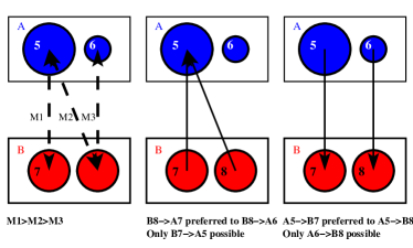
(a) Illustration of an asymmetry leading to a cross-identification inconsistency

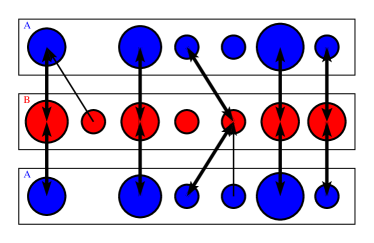
(b) Result after correction

Figure 11.— Illustration of a cross-comparison inconsistency, and possible correction. We ensure that the same answers are obtained after substituting catalog A and B. The configuration illustrated in the left panel is detected in order to obtain the final result displayed in the right panel.

Solving it simply requires ignoring at least one connection. One way to do so is to apply additional conditions for associating halos, or apply a threshold to the merit. For a particle based merit function, we could define a criteria that would render inconsistencies impossible by construction. Let us first denote $f^{X}_{Y}=M_{X\cap Y}/M_{X}$, and suppose our example has the following characteristics: $f^{B7}_{A5}>0.5$, $f^{B8}_{A5}>0.5$ and $f^{A6}_{B8}>0.5$. We have by definition $f^{B8}_{A5}+f^{B8}_{A6}\leq 1$, so $f^{B8}_{A6}<0.5$. Imposing the conditions $f^{X}_{Y}>0.5$ and $f^{Y}_{X}>0.5$, would remove the (A6,B8) connection and the inconsistency itself. By construction we also have $f^{A5}_{B7}+f^{A5}_{B8}\leq 1$. Unless $f^{A5}_{B7}=f^{A5}_{B8}=0.5$, at least one additional connection is removed.

This selection criteria can thus be too severe as it may remove connections that do not lead to inconsistencies. In this paper we used the normalized shared merit function, which translate as $\mathcal{M}_{m}(X,Y)=f^{X}_{Y}\times f^{Y}_{X}$. As we still suppose that $M1>M2$, we have $f^{B7}_{A5}\times f^{A5}_{B7}>f^{B8}_{A5}\times f^{A5}_{B8}$. We still have $f^{B7}_{A5}>0.5$ and $f^{B8}_{A5}>0.5$ and we know that either $f^{A5}_{B7}$ or $f^{A5}_{B8}$ has to be lower than 0.5. We could expect that $f^{B8}_{A5}<0.5$ and that the stronger connection remains. But with $f^{B7}_{A5}$ quite larger than $f^{B8}_{A5}$ ($f^{B7}_{A5}\sim 1$ and $f^{B8}_{A5}\sim 0.5$), we could have $f^{A5}_{B7}<0.5<f^{A5}_{B8}$ while respecting the ordering of the merits. The stronger connection (between A5 and B7) would be removed and only the second best (between A5 and B8) may remain. A more flexible variation of this criteria would be necessary to avoid removing connections one may find important. The conditions $f^{X}_{Y}\geq 0.5$ and $f^{Y}_{X}\geq 0.5$ implies that $\mathcal{M}_{m}(X,Y)\geq 0.25$. This threshold of 0.25 is quite efficient in the most majority of case but it doesn’t rule out either $f^{X}_{Y}<0.5$ or $f^{Y}_{X}<0.5$. This fiducial threshold is not sufficient to avoid all possible issues, but too large a selection threshold would strongly limit the cross-identified catalog.

An alternative approach could be to maximize the number of cross-identified pairs. Since the cross-comparison is structured as a tree, it is straightforward to detect such problematic configurations as illustrated in Figure 11a. Once the pattern is found, one can simply ignore the second connection $M2$ and correct the problem automatically as displayed in Figure 11b. In the end, we favor a cross-identification to a simple association. The advantage of this method is that it is easily applied to any kind of merit functions, whether the criteria is based on distance or on traced mass. The downside is that we may artificially build cross-identifications from low strength connections. For example, we could have $f^{B8}_{A6}<0.1$, which would make $\mathcal{M}_{m}(A6,B8)<0.05$. Applying a threshold on the merit function thus remains relevant even after inconsistencies have been edited out. This is the correction we implemented for this paper. This way we ensure that all inconsistencies are avoided independently of any value we may chose for a merit threshold.

References

- Abazajian et al. (2009) Abazajian, K. N., Adelman-McCarthy, J. K., Agüeros, M. A., et al. 2009, ApJS, 182, 543
- Adelman-McCarthy et al. (2006) Adelman-McCarthy, J. K., Agüeros, M. A., Allam, S. S., et al. 2006, ApJS, 162, 38
- Aubert et al. (2004) Aubert, D., Pichon, C., & Colombi, S. 2004, MNRAS, 352, 376
- Avila et al. (2014) Avila, S., Knebe, A., Pearce, F. R., et al. 2014, MNRAS, 441, 3488
- Baugh (2006) Baugh, C. M. 2006, Reports on Progress in Physics, 69, 3101
- Behroozi et al. (2010) Behroozi, P. S., Conroy, C., & Wechsler, R. H. 2010, ApJ, 717, 379
- Behroozi et al. (2013) Behroozi, P. S., Wechsler, R. H., & Wu, H.-Y. 2013, ApJ, 762, 109
- Berlind & Weinberg (2002) Berlind, A. A., & Weinberg, D. H. 2002, ApJ, 575, 587
- Brenier et al. (2003) Brenier, Y., Frisch, U., Hénon, M., et al. 2003, MNRAS, 346, 501
- Bullock et al. (2002) Bullock, J. S., Wechsler, R. H., & Somerville, R. S. 2002, MNRAS, 329, 246
- Cole et al. (2000) Cole, S., Lacey, C. G., Baugh, C. M., & Frenk, C. S. 2000, MNRAS, 319, 168
- Colless et al. (2001) Colless, M., Dalton, G., Maddox, S., et al. 2001, MNRAS, 328, 1039
- Croton et al. (2006) Croton, D. J., Springel, V., White, S. D. M., et al. 2006, MNRAS, 365, 11
- Cui et al. (2012) Cui, W., Borgani, S., Dolag, K., Murante, G., & Tornatore, L. 2012, MNRAS, 423, 2279
- Cui et al. (2014) Cui, W., Borgani, S., & Murante, G. 2014, MNRAS, 441, 1769
- Cui et al. (2016) Cui, W., Power, C., Biffi, V., et al. 2016, MNRAS, 456, 2566
- Davis et al. (1985) Davis, M., Efstathiou, G., Frenk, C. S., & White, S. D. M. 1985, ApJ, 292, 371
- Diemand et al. (2006) Diemand, J., Kuhlen, M., & Madau, P. 2006, ApJ, 649, 1
- Doumler et al. (2013) Doumler, T., Hoffman, Y., Courtois, H., & Gottlöber, S. 2013, MNRAS, 430, 888
- Gottloeber et al. (2010) Gottloeber, S., Hoffman, Y., & Yepes, G. 2010, ArXiv e-prints, arXiv:1005.2687
- Hanson (2001) Hanson, K. M. 2001, Proc. SPIE, 4322, 456
- Hatton et al. (2003) Hatton, S., Devriendt, J. E. G., Ninin, S., et al. 2003, MNRAS, 343, 75
- Heß et al. (2013) Heß, S., Kitaura, F.-S., & Gottlöber, S. 2013, MNRAS, 435, 2065
- Hoffman & Ribak (1991) Hoffman, Y., & Ribak, E. 1991, ApJ, 380, L5
- Jasche & Wandelt (2013) Jasche, J., & Wandelt, B. D. 2013, MNRAS, 432, 894
- Jing et al. (2002) Jing, Y. P., Börner, G., & Suto, Y. 2002, ApJ, 564, 15
- Jing et al. (1998) Jing, Y. P., Mo, H. J., & Börner, G. 1998, ApJ, 494, 1
- Jing & Suto (2002) Jing, Y. P., & Suto, Y. 2002, ApJ, 574, 538
- Kang et al. (2005) Kang, X., Jing, Y. P., Mo, H. J., & Börner, G. 2005, ApJ, 631, 21
- Kauffmann et al. (1993) Kauffmann, G., White, S. D. M., & Guiderdoni, B. 1993, MNRAS, 264, 201
- Kitaura (2013) Kitaura, F.-S. 2013, MNRAS, 429, L84
- Klypin et al. (2003) Klypin, A., Hoffman, Y., Kravtsov, A. V., & Gottlöber, S. 2003, ApJ, 596, 19
- Knebe et al. (2011) Knebe, A., Knollmann, S. R., Muldrew, S. I., et al. 2011, MNRAS, 415, 2293
- Knollmann & Knebe (2009) Knollmann, S. R., & Knebe, A. 2009, ApJS, 182, 608
- Kravtsov (2003) Kravtsov, A. V. 2003, ApJ, 590, L1
- Kravtsov et al. (2002) Kravtsov, A. V., Klypin, A., & Hoffman, Y. 2002, ApJ, 571, 563
- Kravtsov et al. (1997) Kravtsov, A. V., Klypin, A. A., & Khokhlov, A. M. 1997, ApJS, 111, 73
- Lacey & Cole (1994) Lacey, C., & Cole, S. 1994, MNRAS, 271, 676
- Lavaux (2010) Lavaux, G. 2010, MNRAS, 406, 1007
- Maciejewski et al. (2009) Maciejewski, M., Colombi, S., Springel, V., Alard, C., & Bouchet, F. R. 2009, MNRAS, 396, 1329
- Muñoz-Cuartas et al. (2011) Muñoz-Cuartas, J. C., Müller, V., & Forero-Romero, J. E. 2011, MNRAS, 417, 1303
- Nusser & Dekel (1992) Nusser, A., & Dekel, A. 1992, ApJ, 391, 443
- Onions et al. (2012) Onions, J., Knebe, A., Pearce, F. R., et al. 2012, MNRAS, 423, 1200
- Rodríguez-Puebla et al. (2015) Rodríguez-Puebla, A., Avila-Reese, V., Yang, X., et al. 2015, ApJ, 799, 130
- Scranton (2002) Scranton, R. 2002, MNRAS, 332, 697
- Somerville & Primack (1999) Somerville, R. S., & Primack, J. R. 1999, MNRAS, 310, 1087
- Sorce et al. (2014) Sorce, J. G., Courtois, H. M., Gottlöber, S., Hoffman, Y., & Tully, R. B. 2014, MNRAS, 437, 3586
- Sorce et al. (2016) Sorce, J. G., Gottlöber, S., Yepes, G., et al. 2016, MNRAS, 455, 2078
- Springel (2005) Springel, V. 2005, MNRAS, 364, 1105
- Springel (2010) —. 2010, MNRAS, 401, 791
- Springel et al. (2001a) Springel, V., White, S. D. M., Tormen, G., & Kauffmann, G. 2001a, MNRAS, 328, 726
- Springel et al. (2001b) Springel, V., Yoshida, N., & White, S. D. M. 2001b, LABEL:@jnlNew A, 6, 79
- Srisawat et al. (2013) Srisawat, C., Knebe, A., Pearce, F. R., et al. 2013, MNRAS, 436, 150
- Tassev & Zaldarriaga (2012) Tassev, S., & Zaldarriaga, M. 2012, LABEL:@jnlJ. Cosmology Astropart. Phys., 12, 11
- Taylor et al. (2008) Taylor, J. F., Ashdown, M. A. J., & Hobson, M. P. 2008, MNRAS, 389, 1284
- Teyssier (2002) Teyssier, R. 2002, A&A, 385, 337
- Tweed et al. (2009) Tweed, D., Devriendt, J., Blaizot, J., Colombi, S., & Slyz, A. 2009, A&A, 506, 647
- van den Bosch (2002) van den Bosch, F. C. 2002, MNRAS, 332, 456
- van den Bosch et al. (2003) van den Bosch, F. C., Yang, X., & Mo, H. J. 2003, MNRAS, 340, 771
- Wadsley et al. (2004) Wadsley, J. W., Stadel, J., & Quinn, T. 2004, LABEL:@jnlNew A, 9, 137
- Wang et al. (2009) Wang, H., Mo, H. J., Jing, Y. P., et al. 2009, MNRAS, 394, 398
- Wang et al. (2014) Wang, H., Mo, H. J., Yang, X., Jing, Y. P., & Lin, W. P. 2014, ApJ, 794, 94
- Wang et al. (2012) Wang, H., Mo, H. J., Yang, X., & van den Bosch, F. C. 2012, MNRAS, 420, 1809
- Wang et al. (2013) —. 2013, ApJ, 772, 63
- Wang et al. (2016) Wang, H., Mo, H. J., Yang, X., et al. 2016, ArXiv e-prints, arXiv:1608.01763
- White & Frenk (1991) White, S. D. M., & Frenk, C. S. 1991, ApJ, 379, 52
- Yang et al. (2003) Yang, X., Mo, H. J., & van den Bosch, F. C. 2003, MNRAS, 339, 1057
- Yang et al. (2008) —. 2008, ApJ, 676, 248
- Yang et al. (2009) —. 2009, ApJ, 695, 900
- Yang et al. (2005) Yang, X., Mo, H. J., van den Bosch, F. C., & Jing, Y. P. 2005, MNRAS, 356, 1293
- Yang et al. (2007) Yang, X., Mo, H. J., van den Bosch, F. C., et al. 2007, ApJ, 671, 153
- Yang et al. (2012) Yang, X., Mo, H. J., van den Bosch, F. C., Zhang, Y., & Han, J. 2012, ApJ, 752, 41
- Zel’dovich (1970) Zel’dovich, Y. B. 1970, A&A, 5, 84