Universal continuous transition to turbulence in a planar shear flow

Abstract

We examine the onset of turbulence in Waleffe flow – the planar shear flow between stress-free boundaries driven by a sinusoidal body force. By truncating the wall-normal representation to four modes, we are able to simulate system sizes an order of magnitude larger than any previously simulated, and thereby to attack the question of universality for a planar shear flow. We demonstrate that the equilibrium turbulence fraction increases continuously from zero above a critical Reynolds number and that statistics of the turbulent structures exhibit the power-law scalings of the (2+1)D directed percolation universality class.

1 Introduction

The transition to turbulence in wall-bounded shear flows has been studied for well over a century, and yet, only recently have experiments, numerical simulations, and theory advanced to the point of providing a comprehensive understanding of the route to turbulence in such flows. Of late, research has focused on how turbulence first appears and becomes sustained. The issue is that typically wall-bounded shear flows undergo subcritical transition, meaning that as the Reynolds number is increased, turbulence does not arise through a linear instability of laminar flow, but instead appears directly as a highly nonlinear state. Moreover, the flow does not simply become everywhere turbulent beyond a certain Reynolds number. Rather, turbulence initially appears as localised patches interspersed within laminar flow. The resulting flow takes on a complex spatiotemporal form with competing turbulent and laminar domains. This, in turn, greatly complicates the quantitative analysis of turbulent transition in subcritial shear flows. See Barkley (2016) and Manneville (2016) for recent reviews.

In the 1980s the connection was developed between spatially extended dynamical systems and subcritical turbulent flows. This provided a broad and useful context in which to view turbulent-laminar intermittency. Kaneko (1985) constructed minimal models that demonstrated how dynamical systems with chaotic (“turbulent”) and steady (“laminar”) phases would naturally generate complex spatiotemporal patterns. Simple models were further studied by Chaté & Manneville (1988) amongst others. At the same time, Pomeau (1986) observed that subcritical fluid flows have the characteristics of non-equilibrium systems exhibiting what is known as an absorbing state transition. Based on this, he postulated that these flows might fall into the universality class of directed percolation. This would imply that the turbulence fraction varies continuously with Reynolds number, going from zero to non-zero at a critical Reynolds number, with certain very specific power laws holding at the onset of turbulence. (These concepts will be explained further in §2.) Since then considerable effort has been devoted to investigating these issues. The first experimental observation of directed percolation was reported by Takeuchi et al. (2007, 2009) for electroconvection in nematic liquid crystals.

The status of our understanding for prototypical subcritical shear flows is as follows. For pipe flow, there are extensive measurements of the localized turbulent patches (puffs) that drive the transition to turbulence and we have a good estimate of the critical point for the onset of sustained turbulence (Avila et al., 2011). However, currently there is no experimental or computational measurement of the scalings from which to determine whether the flow is, or is not, in the universality class of directed percolation, although model systems support that the transition is in this class (Barkley, 2011; Shih et al., 2016; Barkley, 2016). The scaling exponents depend on the spatial dimension of the system. Lemoult et al. (2016) recently carried out a study of Couette flow highly confined in two directions so that large-scale turbulent-laminar intermittency could manifest itself only along one spatial dimension. In both experiments and numerical simulations, they measured turbulence fraction as a function of Reynolds number and analysed the spatial and temporal correlations close to the critical Reynolds number. The results support a continuous variation of the turbulence fraction, from zero to non-zero at the onset of turbulence, with scaling laws consistent with the expectations for directed percolation in one spatial dimension.

In systems in which the flow is free to evolve in two large spatial directions, such as Couette and channel flow, the problem is much more difficult and the situation is less clear. Past work has suggested that the turbulence fraction varies discontinuously in plane Couette flow, and hence that transition in the flow is not of directed-percolation type (Bottin & Chaté, 1998; Bottin et al., 1998; Duguet et al., 2010). More recently, Avila (2013) conducted experiments in a counter-rotating circular Couette geometry (radius ratio $\eta=0.98$) of large aspect ratio, and observed a variation of turbulence fraction with Reynolds number suggesting a continuous transition to turbulence. Further investigation would be needed to determine whether the transition is in the universality class of directed percolation. Sano & Tamai (2016) performed experiments on plane channel flow and concluded that this flow exhibits a continuous transition to turbulence in the universality class of directed percolation. However, they report a critical Reynolds number (based on the centerline velocity of the equivalent laminar flow) of $\Rey=830$, whereas other researchers (Xiong et al., 2015; Paranjape et al., 2017; Kanazawa et al., 2017; Tsukahara & Ishida, 2017) observe sustained turbulent patches below 700. These later authors do not address the question of whether the transition is continuous or discontinuous, and further study is needed.

The goal of the present paper is threefold. Firstly, using a coupled-map lattice, we present the essential issues surrounding the onset of turbulence in a spatiotemporal setting, with particular emphasis on the case of two space dimensions. Secondly, we present a numerical study of a planar shear flow of unprecedented lateral extent and show that the onset of turbulence in this flow is continuous and is in the universality class of directed percolation. Finally, we discuss the issue of scales in the current and past studies, and we offer guidance to future investigations.

2 Coupled-map lattices and directed percolation revisited

Before discussing the planar shear flow, we revisit some important issues concerning spatiotemporal intermittency and directed percolation. The issues can most easily be illustrated using a coupled-map-lattice (CML) model. Such discrete-space, discrete-time models have been widely used to study the generic behaviour arising in spatially extended chaotic dynamical systems (e.g. Kaneko, 1985; Chaté & Manneville, 1988; Rolf et al., 1998). Most notably they have been used as minimal models for describing the transition to turbulence in plane Couette flow (Bottin & Chaté, 1998).

The CML model is illustrated in figure 1. A state variable $u$ is defined on a discrete square lattice (figure 1a). Time evolution is given by discrete updates on the lattice. Specifically, letting $u_{ij}$ denote the state variable at point $(i,j)$, the update rule for $u$ is

$$u_{ij}\leftarrow f(u_{ij})+d\triangle_{f}u_{ij}$$ (1)

where the first term, $f(u_{ij})$, is the local dynamics and the second term is a nearest-neighbour diffusive-like coupling. Lattice sites are updated asynchronously by cycling through $(i,j)$ in a random order for each step, as described by Rolf et al. (1998). The control parameter is the coupling strength $d$.

The local dynamics are given by the map $f$ shown in figure 1(b). It has a “turbulent” tent region for $0\leq u\leq 1$ and a “laminar” region $u>1$ surrounding the stable fixed point at $u^{*}$. In the absence of coupling, a turbulent site evolves chaotically and eventually makes a transition to the laminar state. Once a site becomes laminar, it will remain so indefinitely. The laminar fixed point is referred to as an absorbing state. Hence, the local dynamics are a simple caricature of a subcritical shear flow with coexisting turbulent and laminar flow states. Because the model is only a slight generalisation of those appearing in numerous past studies, we relegate the details to the appendix.

Figure 1: Intermittent transition in a coupled map lattice. ($a$) Illustration of the lattice with nodes coloured according to whether the system is locally laminar (white) or turbulent (black). ($b$) The map defining the local dynamics at each node. $u^{*}$ is a stable fixed point. ($c$) Typical time evolution, seen in a slice through the lattice at constant $j$, initialised with all sites in the turbulent state. (The spatial and temporal laminar gaps $\ell_{x}$ and $\ell_{t}$ are discussed in §4.) ($d$) Equilibrium turbulence fraction $F_{t}$ as a function of the coupling strength $d$ in two cases: $u^{*}=1.25$ (top) and $u^{*}=1.1$ (bottom). In the top case the transition to turbulence is discontinuous while in the bottom case it is continuous. In the continuous case, close to the critical value $d_{c}$, $F_{t}$ increases from zero with the universal power law for directed percolation in two space dimensions: $F_{t}\sim(d-d_{c})^{\beta}$, where $\beta\simeq 0.583$. The red curves in the main plot and inset show this power law.

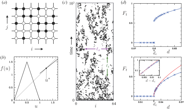
We are primarily interested in the long-time dynamics of the system. We start from an initial condition with randomly selected values within the turbulent region. Figure 1(c) shows the evolution as seen in a one-dimensional slice through the lattice. The main quantity of interest is the turbulence fraction $F_{t}$, which is the fraction of sites in the turbulent state. After some time, the system will reach a statistical equilibrium and we can obtain the equilibrium value of $F_{t}$. If this is zero, then the system is everywhere in the laminar (absorbing) state. If it is non-zero, then at least some turbulence persists indefinitely.

A basic question is: how does the turbulence fraction at equilibrium depend on the coupling strength $d$, and in particular, how does it go from zero to non-zero? Figure 1(d) shows the two distinct cases: one discontinuous and one continuous. In the discontinuous case, there is a gap in the possible values of $F_{t}$. Long-lived transients with small turbulence fraction can be observed for values of $d$ below $d_{c}$, the critical value of $d$, but the system simply cannot indefinitely maintain a small level of turbulence, no matter how large the system size. On the other hand, in the continuous case, $F_{t}$ becomes arbitrarily small (in the limit of infinite system size) as $d$ approaches $d_{c}$ from above. In this case the system behaves in accordance with the power laws of directed percolation. In particular, as is shown, the turbulence fraction grows as $F_{t}\sim(d-d_{c})^{\beta}$, where $\beta\simeq 0.583$; see Lübeck (2004). We will discuss the other important power laws later when we analyse the planar fluid flow.

Note that on any finite lattice the minimum possible non-zero turbulence fraction is 1/$K$, (i.e. just one turbulent site), where $K$ is the total number of lattice points. This means that even if the transition is continuous in principle, some discontinuity in the turbulence fraction from finite-size effects will be present in any numerical study. It is by investigating scaling behaviour, such as the log-log plot in figure 1(d), that one gains confidence in the nature of the transition.

2.1 Connection to turbulent transition and directed percolation

The difference between the continuous and discontinuous cases presented in figure 1(d) is only the location of the laminar fixed point $u^{*}$ in the map $f$. Hence, either case could in principle correspond to a shear flow and there is no way to know a priori what type of transition could be expected. This point was well understood by the Saclay group in their early studies on transition in plane Couette flow (e.g. Bottin & Chaté, 1998; Bottin et al., 1998; Bergé et al., 1998; Manneville, 2016). Those experiments suggested a discontinuous transition to turbulence, based not only on the turbulence fraction, but also on the nature of transients below the critical point. Although we will argue that the physical size of those experiments was too small to produce a continuous transition, the conclusion reached was reasonable at the time.

More generally, directed percolation describes a stochastic process involving active and absorbing states (or equivalently bonds between sites that are randomly open or closed). As Manneville (2016, Section 4.2) notes, deterministic iterations of continuous variables coupled by diffusion will not necessarily behave in the same way as the directed percolation process. The CML model presented here demonstrates this point. Depending on parameters, the system might, or might not, show a continuous transition in the universality class of directed percolation. Notwithstanding Pomeau’s conjecture, it is even less immediately evident that the full Navier–Stokes equations will behave in the same way, owing to the global nature of the pressure field for example. (For more technical details on absorbing state transitions, we refer the reader to Lübeck (2004), and references therein. One can find there details of the Janssen-Grassberger conjecture, (Janssen, 1981; Grassberger, 1982), concerning the ubiquity of the directed percolation universality class.)

From hereon we shall use the notation of directed percolation and refer to the case of two space dimensions as (2+1)-D, meaning two spatial and one temporal dimension. In this notation, the spatial dimensions are referred to as perpendicular ($\perp$) and the temporal dimension as parallel ($\parallel$).

3 Waleffe flow

Pinning down the details of transition requires very large system sizes. For example, in the quasi-one-dimensional experiments of Lemoult et al. (2016), the long direction was more than $2700$ times the fluid gap. Our goal is to achieve something approaching this size, but in two spatial directions and in a computational framework. To this end, we shall study a cousin of Couette flow, commonly referred to as Waleffe flow. This is the shear flow between parallel stress-free boundaries, driven by a sinusoidal body force. The two related computational advantages of this flow are that it lacks high-shear boundary layers near the walls and that the wall-normal dependence of the flow can be accurately represented by a few trigonometric functions. As shown in Chantry et al. (2016), a poloidal-toroidal representation with at most four trigonometric modes in the wall-normal direction, $y$, is capable of capturing turbulent bands and spots, the building blocks of turbulent-laminar intermittency. A Fourier representation is used for the large streamwise, $x$, and spanwise, $z$, directions.

In Chantry et al. (2016), we showed that Waleffe flow corresponds closely to the interior of plane Couette flow, leading to a change in length scales from $2h$ (the gap between walls in plane Couette flow) to $1.25h$ (the Couette interior region) for Waleffe flow. Furthermore, this argument regarding the interior region leads to a comparable velocity scale $U=1.6V$, with $V$ the maximum velocity of laminar Waleffe flow. The Reynolds number of the flow is then $\Rey=Uh/\nu$, where $\nu$ is the kinematic viscosity. The sole change from Chantry et al. (2016) is the addition of a small horizontal drag force $-\sigma(u\mathbf{e}_{x}+w\mathbf{e}_{z})$ to the Navier-Stokes equation. Such a term, usually called Rayleigh or Ekman friction, is used in many hydrodynamic modelling contexts to approximate the effect of friction due to a solid boundary that has been omitted from the model. In geophysics (Marcus & Lee, 1998; Pedlosky, 2012, chap. 4) the inclusion of this term is the standard method of including the first-order departure from geostrophic flow due to the Ekman boundary layer between a stationary bottom and a rotating bulk. In their study of electromagnetically driven Kolmogorov flow in an electrolyte, Suri et al. (2014) include such a term in their depth-averaged model of an assumed Poiseuille-like profile in order to account for the presence in their experiment of a solid boundary at the bottom of the fluid layer.

In our case, we introduce this force in order to damp flows with no curvature in $y$ and very little curvature in $x$ and $z$, which decay extremely slowly in Waleffe flow and which are not present at all in Couette flow. Our purpose is to use Waleffe flow to mimic the bulk region of Couette flow, which it does very well except for this point. The value $\sigma=10^{-2}$ reproduces the damping to which these modes would be subjected in the wall regions of the corresponding Couette flow. In very large domains, without this damping the recovery of the laminar flow after spot decay is very slow. Beyond this, the damping has no effects on the phenomenology of Waleffe flow.

Figure 2: Intermittent turbulence typical of that found slightly above the onset of sustained turbulence. Visualized is streamwise velocity in the midplane at = 173.824 after $1.2\times 10^{6}$ time units. Laminar flow is seen as white. The streamwise and spanwise size of the computational domain is $2560h\times 2560h$. The turbulence fraction is $F_{t}\approx 0.1$ and the reduced Reynolds number is $\epsilon=(Re-Re_{c})/Re_{c}=1.4\times 10^{-4}$. For reference, the Couette domains of Bottin et al. (1998), Duguet et al. (2010), Avila (2013) and Lemoult et al. (2016) are overlaid in red, blue, orange and green respectively. The full streamwise length of the Lemoult et al. (2016) experiment exceeds the figure size and is not fully shown. The spanwise width of the Sano & Tamai (2016) channel experiment is indicated in purple on the right.

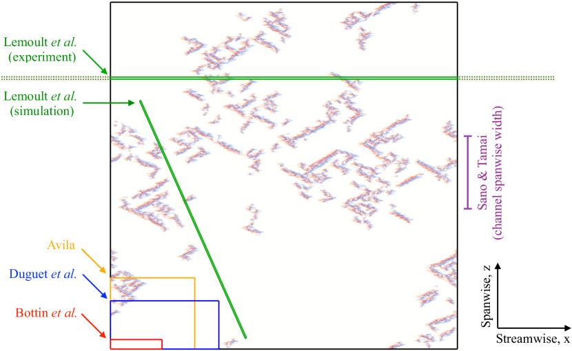
We shall present results for domains of size $[1280h,1.25h,1280h]$, $[2560h,1.25h,2560h]$ and $[5120h,1.25h,1280h]$. Our largest square domain is plotted in figure 2, where we show a representative turbulent state slightly above the onset of turbulence. For this domain the highest resolved wavenumber in each horizontal direction is 2047, with 3/2 dealiasing used (leading to a grid spacing of 0.42). The same turbulence fractions are found in simulations with twice the resolution.

For context, the experiments of Bottin et al. (1998) used a domain of size $[380h,2h,70h]$, Prigent et al. (2003) used a domain of size $[770h,2h,340h]$ and Avila (2013) used a domain of size $[622h,2h,526h]$. To date the largest simulations have been those of Duguet et al. (2010), who considered a domain of size $[800h,2h,356h]$. Both Bottin et al. (1998) and Duguet et al. (2010) report evidence of a discontinuous transition, unable to sustain turbulence fractions significantly below 0.4, while Avila (2013) observed evidence of a continuous transition, with sustained turbulence fractions as small as $0.07$.

The flow at $(x,z,t)$ is defined as turbulent if $E(x,z,t)>E_{T}$, where $E(x,z,t)$ is the $y$-integrated energy of the velocity deviation from the laminar state and $E_{T}=0.01$ is a threshold. Varying $E_{T}$ between 0.001 and 0.05 changes only slightly the size of patches deemed turbulent and has no effect on any of the scaling relationships to follow.

4 Results

Figure 3: (a) Turbulence fraction as function of time for a range of Reynolds numbers with an initial condition of uniform turbulence. Above criticality, the turbulence fraction saturates at a finite value, and below it falls to zero. At criticality, the turbulence fraction decays in time as a power law $F_{t}\sim t^{-\alpha}$ with the (2+1)D directed percolation exponent $\alpha\simeq 0.4505$ (dashed line). Coloured lines, for decreasing turbulence fractions correspond to Reynolds numbers $[173.952,173.888,173.840,173.824,173.792,173.773,173.696,173.568]$. (b) Data above and below criticality collapse onto two scalings (black dashed curves) when the directed percolation exponents are used to rescale time and turbulence fraction.

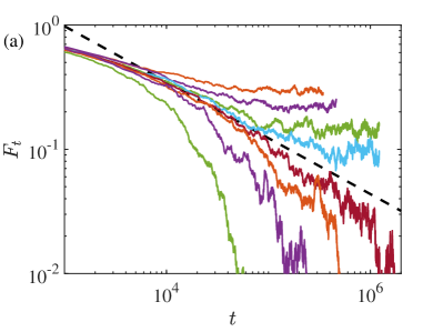
In figure 3(a), we plot the time evolution of the turbulence fraction $F_{t}$ for a series of Reynolds numbers. Each run was initialised from uniform turbulence and run until a saturated turbulence fraction was reached (quench protocol, see Bottin & Chaté, 1998). Below a critical value $\Rey_{c}=173.80$ (to five significant figures), the turbulence fraction eventually falls off to zero, while above $\Rey_{c}$ it saturates at a finite value. ($\Rey_{c}$ for this system differs from that of plane Couette flow).

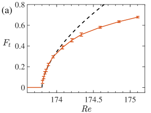
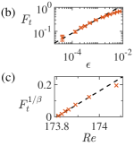
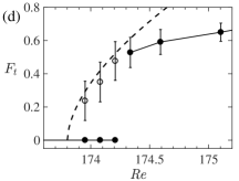
In figure 4(a) we plot the equilibrium turbulence fraction as a function of $\Rey$. We find clear evidence for a continuous transition in which small $F_{t}$ can be sustained given a sufficiently large domain. The saturated turbulence fraction follows a power law $F_{t}\sim\epsilon^{\beta}$ where $\epsilon\equiv(\Rey-\Rey_{c})/\Rey_{c}$. $\Rey_{c}$ is determined as the value of $\Rey$ that minimises the mean squared error of a linear fit of the logarithms of $\epsilon$ and $F_{t}$ (see figure 4b). This linear fit estimates $\beta=0.58\pm 0.04$ with a $95\%$ confidence interval. This agrees with the (2+1)-D directed percolation value $\beta\simeq 0.583$ (dashed line). Figure 4(d) shows the turbulence fraction obtained from our system in a domain whose size is that of the experiments of Bottin & Chaté (1998). (See also figure 2.) As was observed experimentally, below a turbulence fraction of about $0.5$, turbulence appears only as a long-lived transient state, and hence the equilibrium turbulence fraction exhibits a discontinuous transition. This strongly suggests that the discontinuous transitions reported for plane Couette flow (Bottin & Chaté, 1998; Bottin et al., 1998; Duguet et al., 2010) are due to finite-size effects. Interestingly, long-lived transient states in the small system have turbulence fractions close to those for equilibrium states in our large domain; they just are not sustained states. Also note that the critical Reynolds number is not greatly affected by system size.

Figure 4: Bifurcation diagrams for the transition to turbulence. (a) Continuous transition in a large domain: $[2560h,1.25h,2560h]$. Equilibrium turbulence fraction $F_{t}$ is plotted as a function of $\Rey$. Points and error bars denote mean and standard deviation of $F_{t}$. Black dashed curved shows the directed percolation power law. (b) Log-log plot of the same data in terms of $\epsilon=\left(\Rey-\Rey_{c}\right)/{\Rey_{c}}$, where $\Rey_{c}=173.80$. Near criticality the data is consistent with $F_{t}\sim\epsilon^{\beta}$ with $\beta\simeq 0.583$. (c) $F^{1/\beta}$ against $\Rey$ showing linear behaviour. (d) Discontinuous transition in a domain of size $[380h,1.25h,70h]$, approximately that of the experiments by Bottin & Chaté (1998). (See figure 2.) Filled points denote sustained turbulence, while open points denote the turbulence fraction of long-lived transient turbulence. The dashed curve is the directed-percolation power law from the large domain.

Figure 5: Exponents for temporal and spatial correlations. Top row shows distributions of laminar gaps in (a) time and the two spatial directions, (b) $x$ and (c) $z$, for a variety of domain sizes at $\Rey=173.824$ ($\epsilon=1.4\times 10^{-4}$). $N$ is the gap count, normalised by the shortest gap count. The directed percolation scalings ($\mu_{\parallel}\simeq 1.5495$ and $\mu_{\perp}\simeq 1.204$) are plotted as dashed lines and show excellent agreement with the $t$ and $z$ gaps. For the $x$-gaps a power law closer to $-1$ is observed. Middle row, (d-f), shows the exponential tails of the gap distributions for a several values of $\epsilon$ just above criticality. Increasing domain sizes are used for points closer to criticality. Insets show scaling of correlation lengths $\xi$ with $\epsilon$ together with the directed percolation exponents: $\nu_{\parallel}\simeq 1.295$ and $\nu_{\perp}\simeq 0.733$. Bottom row, (g-i), collapse of the data using directed percolation power laws $\mu$ and $\nu$ (see axis labels/text).

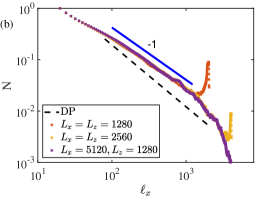
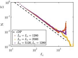
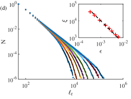
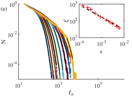
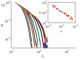
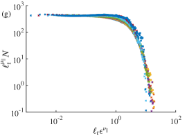
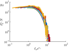
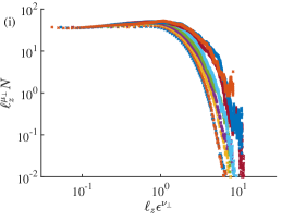
To substantiate whether a system is in the directed percolation universality class, it is necessary to verify three independent power-law scalings close to criticality; see Takeuchi et al. (2009) whose approach we will follow closely. Having demonstrated the scaling of $F_{t}$ (exponent $\beta$), we now turn to scalings associated with temporal and spatial correlations.

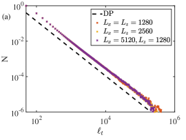
One approach to determining the correlations is via the distribution of laminar gaps at $\Rey\simeq\Rey_{c}$, (top row of figure 5). The flow has a temporal laminar gap of length $\ell_{t}$ if $E(x,z,t)>E_{T}$ and $E(x,z,t+\ell_{t})>E_{T}$ but $E(x,z,t^{\prime})<E_{T}$ for $0<t^{\prime}<\ell_{t}$. Spatial gaps $\ell_{x}$ and $\ell_{z}$ are defined similarly. Such gaps are illustrated for the CML model in figure 1(c). From simulations just above $\Rey_{c}$, we generate gap distributions by measuring and binning the laminar gaps within the intermittent flow once the turbulence fraction has saturated. Given the anisotropy between the streamwise and spanwise directions, we measure gaps in these directions separately. At criticality, a system within the directed-percolation universality class displays power-law behaviour, $N\sim\ell^{-\mu}$, where $N$ is the number of gaps of length $\ell$. The temporal gaps, figure 5(a), show excellent scaling with the directed-percolation temporal exponent $\mu_{\parallel}\simeq 1.5495$ This is also true of the spanwise gaps, figure 5(c), with the spatial exponent $\mu_{\perp}\simeq 1.204$. However, the streamwise laminar gaps, figure 5(b), do not show a clear, extended power law, and to the extent that there is a power law, the exponent is closer to 1 than to $\mu_{\perp}\simeq 1.204$. Indeed, Takeuchi et al. (2007) observed that the laminar gap distribution in one direction of a liquid crystal layer had an exponent closer to 1 than to $\mu_{\perp}\simeq 1.204$, This is also true for our simulations of a non-isotropic CML very slightly above the critical point, thus indicating that the issue here is that the flow is not exactly at $\Rey_{c}$, as it should be for the scaling to hold. Although the gap distribution in each spatial direction should show power-law behaviour, these may converge at different rates as $\Rey\rightarrow\Rey_{c}$.

Given the poor agreement for the streamwise gaps, we use a second approach to measure the percolation exponents which does not rely on simulations at $\Rey_{c}$. Away from criticality, power-law behaviour will be seen only over a finite range of temporal and spatial gap lengths. Beyond these lengths, exponential tails are expected of the form $N\sim\exp(-\ell/\xi)$, with correlation lengths $\xi$ diverging as $\epsilon$ goes to zero: $\xi\sim\epsilon^{-\nu}$. In the middle row of figure 5 we fit exponential tails for several values of $\epsilon$. In the insets we plot $\xi$ as a function of $\epsilon$ and compare with the expected exponents for directed percolation. The exponents $\mu$ and $\nu$ are exactly related via $\mu=2-\beta/\nu$, thus giving $\nu_{\parallel}\simeq 1.295$ and $\nu_{\perp}\simeq 0.733$ (Lübeck, 2004). Because the exponents $\mu$ and $\nu$ are linked, the power laws in the middle row of figure 5 are not independent of the corresponding power laws in the top row. However, they rely on different data and hence are not limited by the same finite-size and finite-distance-from-critical effects. The power law for the $x$ direction is now seen to be in clear agreement with the directed percolation exponent, as are those in $t$ and $z$.

Combining these power laws, the laminar gap distributions can be collapsed using the relationship $N\ell^{\mu}=G(\ell\epsilon^{\nu})$, where $G$ is an unknown function (Henkel et al., 2008, pp. 111-112). In the bottom row of figure 5 we plot our data in collapsing coordinates using the (2+1)-D percolation exponents. This collapse is well illustrated by the temporal gap distribution, a culmination of the excellent fits of $\mu_{\parallel}$ and $\nu_{\parallel}$. For the $x$-gaps, only gaps of length 100 or greater are counted, corresponding to the start of the power law in figure 5(b). The collapse of the $z$-gaps is hindered by the $\nu_{\perp}$ scaling seen in figure 5(f), but close to criticality (last three lines) the data begin to show collapse.

We have also run simulations in a quasi-1D, streamwise-oriented domain similar in spirit to the experiments of Lemoult et al. (2016) (see the experimental domain in figure 2). In a domain of size $[1280h,1.25h,40h]$, the distribution of streamwise laminar gaps near criticality exhibits a clear power law, in contrast to the poor power-law behaviour found for streamwise laminar gaps in the full planar system (figure 5b). The exponent is $\mu_{\perp}\simeq 1.748$, as predicted for systems with a single spatial dimension ((1+1)D directed percolation).

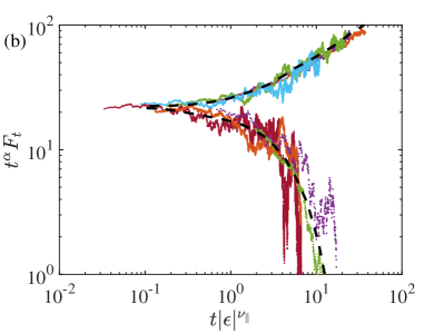
We return to the time evolution shown in figure 3 (a). Between the evolution at $\Rey<\Rey_{c}$ and $\Rey>\Rey_{c}$ is the power law decay predicted for a directed-percolation process at criticality: $F_{t}\sim t^{-\alpha}$, where $\alpha=2-\mu_{\parallel}\simeq 0.4505$. Close to criticality, we observe evidence for this power law in the data. This plot highlights a major challenge to simulations near criticality – well over $10^{5}$ time units are required to reach even the moderately small turbulence fractions simulated here. As was noted by Avila (2013, p. 32), these long timescales proved an issue in the work of Duguet et al. (2010), who in $10^{4}$ time units of simulation were unable to converge turbulence fractions much below 0.4. As in the present study, Avila (2013, p. 90) let the system evolve for $O(10^{6})$ advective time units close to transition. Hence both simulation time and domain size can be limiting factors in observing the hallmarks of percolation. Using directed percolation scalings (Takeuchi et al., 2009), the data above and below criticality collapse onto two curves (figure 3b), highlighting the universality of directed percolation in the transition to turbulence.

5 Discussion

Over the years several attempts have been made to quantify the transition to turbulence and to determine whether or not subcritical shear flows follow the spatiotemporal scenario of directed percolation. Such attempts have consistently been frustrated by the large system sizes required to address the issue. Here we have performed simulations of a planar flow of sufficient size that we have been able to eliminate significant finite-size, finite-time effects, and thereby to examine in full detail the onset of turbulence in a planar example. We have demonstrated both that the equilibrium turbulence fraction increases continuously from zero above a critical Reynolds number and that statistics of the turbulent structures exhibit the power-law scalings of the directed percolation universality class. Meeting such demands has necessitated not only turning to the stress-free boundaries of Waleffe flow, but further truncating the simulations to just four wall-normal modes. Performing a comparable computational study directly on plane Couette flow is currently far beyond available resources.

In light of what we now understand about the scales needed to capture sparse turbulent structures near the onset of turbulence, we have re-examined the apparent discontinuous transition to turbulence reported in past studies of plane Couette flow. The conclusions of those studies were reasonable at that time, but our results indicate that prior experimental system sizes were too small, and prior simulation times were too short, to accurately capture sustained turbulence close to onset – both space and time constraints can limit estimates of true equilibrium dynamics. Apart from overall issues of scale, we have observed that the scaling relations in the streamwise and spanwise directions may converge at different rates. Because shear flows are non-isotropic, it is important to monitor these directions separately. These considerations should guide the design of experiments and computations. In this regard, it should be noted that while the Reynolds numbers in our study differ from those of plane Couette flow, the length and time scales are closely comparable to those of plane Couette flow. The efficiency with which our system can be simulated offers potential for use in conjunction with future investigation.

While we cannot rule out the possibility that other subcritical shear flows follow some different route to turbulence, we know that truncated Waleffe flow contains the essential self-sustaining mechanism of wall-bounded turbulence and that it produces the oblique turbulent bands that characterize transitional turbulence in plane Couette and plane channel flow (Chantry et al., 2016). The closeness of these phenomena suggests that all of these flows exhibit the same route to turbulence.

Appendix. Details of the CML

We provide here details of the CML model and simulations shown in §2. For the most part, these follow previous works (e.g. Bottin & Chaté, 1998; Rolf et al., 1998). The local dynamics is given by the map $f$:

$$f(u)=\begin{cases}ru,&u\leq 1/2\\ r(1-u)&1/2<u\leq 1\\ k(u-u^{*})+u^{*}&1<u\end{cases}$$ (2)

where $r$, $k$, and $u^{*}$ are parameters. Here we fix $r=3.0$ and $k=0.8$. The only difference between this map and those used previously is that here $u^{*}$ is a free parameter, rather than being set by the value of $r$ to $u^{*}=(r+2)/4$.

The spatial coupling is given by

$$\triangle_{f}u_{ij}= \frac{1-\delta}{4}\left(f(u_{i-1,j})-2f(u_{i,j})+f(u_{i+1,j})\right)$$

$$+ \frac{1+\delta}{4}\left(f(u_{i,j-1})-2f(u_{i,j})+f(u_{i,j+1})\right)$$

subject to periodic boundary conditions. This term differs from the standard coupling only in that the parameter $\delta$ permits different coupling strengths in the $i$ and $j$ directions, to mimic the anisotropy of planar shear flows. We use $\delta=0.6$. This anisotropy has no significance for the results presented in this paper since continuous and discontinuous transitions occur also in the isotropic case $\delta=0$. We show results at $\delta=0.6$ only for consistency with future publications.

References

- Avila (2013) Avila, K. 2013 Shear flow experiments: Characterizing the onset of turbulence as a phase transition, PhD thesis, Georg-August University School of Science.
- Avila et al. (2011) Avila, K., Moxey, D., de Lozar, A., Avila, M., Barkley, D. & Hof, B. 2011 The onset of turbulence in pipe flow. Science 333, 192–196.
- Barkley (2011) Barkley, D. 2011 Simplifying the complexity of pipe flow. Phys. Rev. E 84, 016309.
- Barkley (2016) Barkley, D. 2016 Theoretical perspective on the route to turbulence in a pipe. J. Fluid Mech. 803, P1.
- Bergé et al. (1998) Bergé, P., Pomeau, Y. & Vidal, C. 1998 L’espace Chaotique. Hermann Éd. des Sciences et des Arts.
- Bottin & Chaté (1998) Bottin, S. & Chaté, H. 1998 Statistical analysis of the transition to turbulence in plane Couette flow. Eur. Phys. J. B 6, 143–155.
- Bottin et al. (1998) Bottin, S., Daviaud, F., Manneville, P. & Dauchot, O. 1998 Discontinuous transition to spatiotemporal intermittency in plane Couette flow. Europhys. Lett. 43, 171–176.
- Chantry et al. (2016) Chantry, M., Tuckerman, L. S. & Barkley, D. 2016 Turbulent–laminar patterns in shear flows without walls. J. Fluid Mech. 791, R8.
- Chaté & Manneville (1988) Chaté, H. & Manneville, P. 1988 Spatio-temporal intermittency in coupled map lattices. Physica D 32, 409–422.
- Duguet et al. (2010) Duguet, Y., Schlatter, P. & Henningson, D. S. 2010 Formation of turbulent patterns near the onset of transition in plane Couette flow. J. Fluid Mech. 650, 119–129.
- Grassberger (1982) Grassberger, P. 1982 On phase transitions in Schlögl’s second model. Z. Physik B - Condensed Matter 47, 365–374.
- Henkel et al. (2008) Henkel, M., Hinrichsen, H., Lübeck, S. & Pleimling, M. 2008 Non-equilibrium Phase Transitions, , vol. 1. Springer.
- Janssen (1981) Janssen, H.-K. 1981 On the nonequilibrium phase transition in reaction-diffusion systems with an absorbing stationary state. Z. Physik B - Condensed Matter 42, 151–154.
- Kanazawa et al. (2017) Kanazawa, T., Shimizu, M. & Kawahara, G. 2017 Presented at KITP Conference: Recurrence, Self-Organization, and the Dynamics of Turbulence, 9-13 January 2017, Kavli Institute for Theoretical Physics. http://online.kitp.ucsb.edu/online/transturb-c17/kawahara/.
- Kaneko (1985) Kaneko, K. 1985 Spatiotemporal intermittency in coupled map lattices. Progr. Theor. Exp. Phys. 74, 1033–1044.
- Lemoult et al. (2016) Lemoult, G., Shi, L., Avila, K., Jalikop, S. V., Avila, M. & Hof, B. 2016 Directed percolation phase transition to sustained turbulence in Couette flow. Nat. Phys. 12, 254–258.
- Lübeck (2004) Lübeck, S. 2004 Universal scaling behavior of non-equilibrium phase transitions. Int. J. Mod. Phys. B 18, 3977–4118.
- Manneville (2016) Manneville, P. 2016 Transition to turbulence in wall-bounded flows: Where do we stand? Bull. JSME 3, 15–00684.
- Marcus & Lee (1998) Marcus, P. & Lee, C. 1998 A model for eastward and westward jets in laboratory experiments and planetary atmospheres. Phys. Fluids 10, 1474–1489.
- Paranjape et al. (2017) Paranjape, C., Vasudevan, M., Duguet, Y. & Hof, B. 2017 Presented at KITP Conference: Recurrence, Self-Organization, and the Dynamics of Turbulence, 9-13 January 2017, Kavli Institute for Theoretical Physics. http://online.kitp.ucsb.edu/online/transturb-c17/hof/rm/jwvideo.html.
- Pedlosky (2012) Pedlosky, J. 2012 Geophysical Fluid Dynamics. Springer Science & Business Media.
- Pomeau (1986) Pomeau, Y. 1986 Front motion, metastability and subcritical bifurcations in hydrodynamics. Physica D 23, 3–11.
- Prigent et al. (2003) Prigent, A., Grégoire, G., Chaté, H. & Dauchot, O. 2003 Long-wavelength modulation of turbulent shear flows. Physica D 174, 100–113.
- Rolf et al. (1998) Rolf, J., Bohr, T. & Jensen, M. 1998 Directed percolation universality in asynchronous evolution of spatiotemporal intermittency. Phys. Rev. E 57, R2503.
- Sano & Tamai (2016) Sano, M. & Tamai, K. 2016 A universal transition to turbulence in channel flow. Nat. Phys. 12, 249–253.
- Shih et al. (2016) Shih, H., Hsieh, T. & Goldenfeld, N. 2016 Ecological collapse and the emergence of travelling waves at the onset of shear turbulence. Nat. Phys. 12, 245–248.
- Suri et al. (2014) Suri, B., Tithof, J., Mitchell Jr, R., Grigoriev, R. O. & Schatz, M. F. 2014 Velocity profile in a two-layer Kolmogorov-like flow. Phys. Fluids 26, 053601.
- Takeuchi et al. (2007) Takeuchi, K. A., Kuroda, M., Chaté, H. & Sano, M. 2007 Directed percolation criticality in turbulent liquid crystals. Phys. Rev. Lett. 99, 234503.
- Takeuchi et al. (2009) Takeuchi, K. A., Kuroda, M., Chaté, H. & Sano, M. 2009 Experimental realization of directed percolation criticality in turbulent liquid crystals. Phys. Rev. E 80, 051116.
- Tsukahara & Ishida (2017) Tsukahara, T. & Ishida, T. 2017 private communication.
- Xiong et al. (2015) Xiong, X., Tao, J., Chen, S. & Brandt, L. 2015 Turbulent bands in plane-Poiseuille flow at moderate Reynolds numbers. Phys. Fluids 27, 041702.