Underapproximation of Reach-Avoid Sets for Discrete-Time Stochastic Systems via Lagrangian Methods
Abstract
We examine Lagrangian techniques for computing underapproximations of finite-time horizon, stochastic reach-avoid level-sets for discrete-time, nonlinear systems. We use the concept of reachability of a target tube in the control literature to define robust reach-avoid sets which are parameterized by the target set, safe set, and the set in which the disturbance is drawn from. We unify two existing Lagrangian approaches to compute these sets and establish that there exists an optimal control policy of the robust reach-avoid sets which is a Markov policy. Based on these results, we characterize the subset of the disturbance space whose corresponding robust reach-avoid set for the given target and safe set is a guaranteed underapproximation of the stochastic reach-avoid level-set of interest. The proposed approach dramatically improves the computational efficiency for obtaining an underapproximation of stochastic reach-avoid level-sets when compared to the traditional approaches based on gridding. Our method, while conservative, does not rely on a grid, implying scalability as permitted by the known computational geometry constraints. We demonstrate the method on two examples: a simple two-dimensional integrator, and a space vehicle rendezvous-docking problem.
I Introduction
Reach-avoid analysis is an established verification tool that provides formal guarantees of both safety (via avoiding unsafe regions) and performance (via reaching a target set). It has been used in safety-critical or expensive systems, for example, with application to space systems [1], aviation [2, 3], biomedical systems [4], and other domains [5, 6, 7]. The reach-avoid set is the set of initial states for which there exists control that enables the state to reach a target within some finite time horizon, while remaining within a safe set (avoiding an unsafe set) for all instants in the time horizon. In a probabilistic system, satisfaction of the reach-avoid objective is accomplished stochastically. The stochastic reach-avoid level-set for a given likelihood is the set of states for which probabilistic success of the reach-avoid objective is assured with at least the given likelihood.
The theoretical framework for the probabilistic reach-avoid calculation is based on dynamic programming [8, 7], and, hence, is computationally infeasible for even moderate-sized systems due to the gridding of not only the state-space, but also of the input and disturbance spaces [9]. Recent work has focused on alternatives to dynamic programming, including approximate dynamic programming [10, 11, 6], Gaussian mixtures [11], particle filters [1, 6], and convex chance-constrained optimization [1, 5]. These methods have been applied to systems that are at most 10-dimensional, at high memory and computational costs [6]. Further, since an analytical expression of the value function is not accessible, stochastic reach-avoid level-sets can be computed only up to the accuracy of the gridding.
We propose a method to compute an underapproximation of probabilistic reach-avoid sets via robust reach-avoid sets, the set of states assured to reach the target set and remain in the safe region despite any disturbance input. Robust reach-avoid sets can be theoretically posed as the solution to the reachability of a target tube problem [12, 13, 14], originally framed to compute reachable sets of discrete-time controlled systems with bounded disturbance sets. Motivated by the scalability of the Lagrangian method proposed in [4, 15] for viability analysis in deterministic systems (that is, systems without a disturbance input but with a control input), we seek a similar approach to compute the robust reach-avoid sets via tractable set theoretic operations. Lagrangian methods rely on computational geometry, whose scalability depends on the representation and the operation used [16], including polyhedrons (implementable using Model Parametric Toolbox (MPT) [17]), support functions [18], and ellipsoids (implementable via the Ellipsoidal Toolbox [19]).
In this paper, we unify these two approaches to create an efficient algorithm for underapproximation of the stochastic reach-avoid set, and demonstrate our approach on practical examples. Our main contributions are: a) synthesis of the approaches presented in [4, 15] and [12, 13, 14] to compute the robust reach-avoid sets, b) sufficient conditions under which an optimal control policy for a given robust reach-avoid set is a Markov policy, and c) an algorithm to compute an underapproximation of the stochastic reach-avoid level-sets using the robust reach-avoid sets. Specifically, we establish the sufficient conditions under which an optimal control policy is comprised of universally measurable state-feedback laws. For these conditions, we characterize the subset of the disturbance space whose corresponding robust reach-avoid set is a guaranteed underapproximation of the desired stochastic reach-avoid level-set. Leveraging established Lagrangian methods, we demonstrate that our approach dramatically reduces the computation time required for computing a conservative underapproximation of the desired stochastic reach-avoid level-set. Further, the Lagrangian methods does not rely on grids, freeing the underapproximated sets from any numerical artifacts arising due to the discretization.
The remainder of the paper is as follows: Section II describes the problem and the necessary notation. In Section III, we describe the relationship between the the recursion established in [12] for the robust reach-avoid set and the Lagrangian approach in [4], and establish the desired measurability properties of the optimal controller. We present an algorithm for underapproximation of stochastic reach-avoid level-sets in Section IV. We demonstrate our algorithm on two examples—a simple two-dimensional integrator and a space vehicle rendezvous-docking problem—in Section V and provide conclusions and directions of future work in Section VI.
II Problem Statement
The following notation will be used throughout the paper: we denote discrete-time time intervals by for ; the set of natural numbers (including zero) as ; the Minkowski sum of two sets as ; the Minkowski difference (or Pontryagin difference) of two sets as ; and the indicator function corresponding to a set as where if and is zero otherwise.
II-A System formulation
We consider a discrete-time, nonlinear, time-invariant system with an affine disturbance,
| (1) |
with state , input , disturbance , and a function . Without loss of generality, we assume contains , the zero vector of . We will also consider the discrete, LTI system of form
| (2) |
for some matrices and . We assume is non-singular, which holds true for discrete-time systems that arise from the discretization of continuous-time systems.
II-B Robust reach-avoid sets
Let and denote the set of admissible state-feedback laws, . We define a control policy as a sequence of state-feedback laws, with for . We denote the corresponding set of admissible control policies as .
Let be a subset of the disturbance set. We define the -time robust reach-avoid set corresponding to as the set of initial states such that there exists an admissible control policy that ensures remains in a safe set for and lies in a target set (reach-avoid objective) despite the presence of the disturbance at each instant. Denoting , the -time robust reach-avoid set is
| (3) |
Note that for , the system (1) is equivalent to a deterministic, discrete-time, nonlinear system
| (4) |
when . The -time viable set of the system (4) is the set of initial states such that there exists an admissible control policy such that remains in a safe set for . That is,
| (5) | ||||
| (6) |
The authors in [4] presented a Lagrangian formulation to compute and discussed the scalability of the viability analysis using MPT, ET, and support functions.
II-C Stochastic reach-avoid level-sets
In this subsection, we further assume the disturbance in (1) is an -dimensional random vector defined in the probability space . Here, denotes the minimal -algebra associated with the random vector . We assume the disturbance is absolutely continuous with a probability density function (PDF) , the disturbance process is an independent and identically distributed (i.i.d.) random process, and is a finite time horizon. We assume that is Borel-measurable, is compact, the sets are Borel, and is continuous.
We denote the set of universally measurable state-feedback laws as . We define the Markov control policy as where , and is the set of admissible Markov policies. Since no measurability restrictions were imposed on the feedback laws in Section II-B, and .
Given a Markov policy and initial state , the concatenated state vector for the system (1) is a random vector defined in the probability space . The probability measure is induced from the probability measure via (1) [7]. We will denote the probability space associated with the random vector as for .
For stochastic reachability analysis, we are interested in the maximum likelihood that the system (1) starting at an initial state will achieve the reach-avoid objective using a Markov policy. The maximum likelihood and the optimal Markov policy can be determined as the solution to the optimization problem, [7]
| (7) |
A dynamic programming approach was presented in [7] to solve problem (7). Let the optimal solution to problem (7) be , the maximal Markov policy in the terminal sense [7, Def. 10]. The existence of a Markov policy is guaranteed for a continuous and compact [20, Thm. 1]. The approach in [7] generates value functions for ,
| (8) |
initialized with
| (9) |
By definition, the optimal value function provides the maximum likelihood, optimal value of problem (7), of achieving the reach-avoid objective by the system (1) for the time horizon and the initial state .
For and , the stochastic reach-avoid -level-set,
| (10) |
is the set of states that achieve the reach-avoid objective by the time horizon with a probability of, at minimum, , in the time interval .
II-D Problem statements
The following problems are addressed in this paper:
Problem 1.
Problem 2.
Problem 3.
III Robust Reach-Avoid Set Computation
In this section, we characterize the robust reach-avoid set for the system described in (1). To solve Problem 1, we first extend the approach presented in [4, 15] to reproduce the results presented in [12]. The authors in [4] demonstrated scalability of the Lagrangian methods for viability analysis in deterministic systems. By unifying these approaches, we aim for a tractable and efficient Lagrangian computation of the robust reach-avoid set with established scalability properties. We also demonstrate that the recursion presented for the viable set computation in deterministic system [4] is a special case of the proposed Lagrangian approach. Finally, we solve Problem 2 and establish that there is an optimal control policy for the robust reach-avoid set that is also a Markov policy.
III-A Iterative computation for robust reach-avoid sets
Similar to the work in [4], for the system (1), we define the unperturbed, one-step forward reach set from a point as , and the unperturbed, one-step backward reach set from a set as . Formally, for the system (1),
| (11) | ||||
| (12) |
where (12) follows from (11). For the system (2),
| (13) | ||||
| (14) |
Proposition 1.
Given a set , the finite horizon robust reach-avoid sets for the system (1) can be computed recursively as follows for :
| (15) | ||||
| (16) |
Proof: We first show the case , which differs slightly from other cases. From (1) and (3),
For any , from (3),
| (17) |
Using (17), we construct in the form of (16).
| (18) | |||
| (19) | |||
Since the choice of depends only , the terms and can be exchanged in (18). We obtain (19) after exchanging the terms and applying (17).
Theorem 1.
For the system given in (1), the finite-time robust reach-avoid sets can be computed using the recursion for :
| (20) | ||||
| (21) |
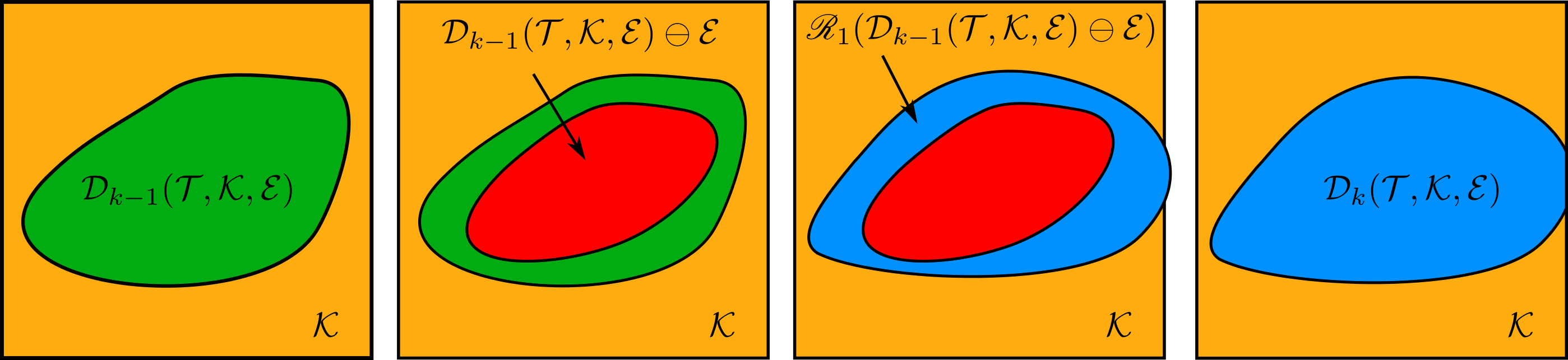
Figure 1 depicts the recursion in Theorem 1 (21) graphically. From (21), we have the following corollary.
Corollary 1.
.
For completeness, we establish that the viability analysis presented in [4] is a special case of Theorem 1. From [21, Theorem 2.1], for any , . Hence,
| (22) |
Corollary 2.
A similar recursion can be provided for computing the reach-avoid sets for a deterministic system.
Lemma 1.
Note that convexity of does not require convexity of . Further, for polyhedral , the robust reach-avoid set is polyhedral for . Note that the same can not be said be for ellipsoids [12, Sec. 4]. A detailed discussion for the implementation of Theorem 1 for polyhedral sets using support functions is given in [12, App. A].
III-B Minmax problem for robust reach-avoid set computation
We will now address Problem 2. A minmax optimization problem was presented in [12, Sec. 1], [22, Sec. 4.6.2] to compute the robust reach-avoid sets (3) for the system (1). The optimization problem is:
| (29) |
where the decision variables are and . Here, for and . The objective function is parameterized by the initial state and the time horizon . Problem (29) can be solved using dynamic programming [22, Sec 1.6] to generate the value functions for
| (30) | ||||
| (31) |
initialized with . The optimal value of problem (29) when starting at is . Further,
| (32) |
Recall that lower semi-continuous functions are functions whose sublevel-sets are closed and upper-semicontinuous functions are functions whose negative is a lower semi-continuous function [23, Definition 7.13]. Also, the supremum of a lower-semicontinuous function is the negative of the infimum of an upper-semicontinuous function. Let an optimal control policy for problem (29) be . Note that need not be unique.
Theorem 2.
For closed sets and compact set , there exists an optimal policy for problem (29) which is also a Markov policy.
Proof: We show by induction that the statement S: the optimal value functions of (29) are lower-semicontinuous and there exists a Borel-measurable state-feedback law for every . Since Borel-measurability implies universal measurability [23, Definition 7.20], the proof of Theorem 2 follows from S and the definition of a Markov policy.
Proof of S: The closedness property of imply is lower semi-continuous for . Hence, is lower-semicontinuous.
Consider the base case . From [23, Prop. 7.32 (b)], we can see that is lower semi-continuous. From [23, Prop. 7.33], we conclude that is lower semi-continuous and an optimal state-feedback policy exists which is also Borel-measurable.
Let . Assume, for induction, the case is true, i.e, is lower semi-continuous. The proof that is lower semi-continuous and the existence of a Borel-measurable follows from [23, Prop. 7.32(b) and 7.33]. This completes the induction.
IV Conservative Approximation of Stochastic Reach-Avoid Level-Set
We will now focus on the stochastic system described in Section II-C and use the theory developed in Section III to solve Problems 3 and 3a.
Theorem 3.
Given closed sets , compact set and a set . For every with ,
| (33) |
Theorem 4.
Given , closed sets , and a compact set , if for any , such that for all , then .
Proof: The case for follows trivially from (9), (10), and (15). Let and . We are interested in underapproximating as defined in (10). From (8),
| (34) | |||
| (35) |
Equation (34) follows from the law of total probability and Corollary 1 which implies . Equation (35) follows from (34) after ignoring the second term (which is non-negative). Simplifying (35) using Theorem 3 and the i.i.d. assumption of the disturbance process, we obtain
| (36) |
Thus, by (10).
Theorem 4 solves Problem 3 for an arbitrary density . Computation of can be done via Theorem 1. Note that characterized by Theorem 4 is not unique. Recall that Corollary 2 states that the robust reach-avoid set is exact viable set for the case when . We therefore prescribe that contains and has the least Lebesgue measure to reduce the the degree of conservativeness in Theorem 4. We also recommend the set be convex and compact for computational ease.
Next, we provide a method to compute for any such that for all when the disturbance in the system (1) is a Gaussian random vector.
IV-A Computation of for Gaussian disturbance
Let the disturbance in (1) be , an -dimensional Gaussian random variable with mean vector and covariance matrix . The probability density of a multivariate Gaussian random vector is [24, Ch. 29]
Consider the -dimensional ellipsoid parameterized by for ,
| (37) |
For , we have , an -dimensional hypersphere of radius . We aim to compute the parameter such that for application of Theorem 4.
Given a standard normal distributed -dimensional random vector , [24, Ch. 29]. Also, with . Since the affine transformation of to is deterministic, . From [24, Ex. 20.16], we have
where is a chi-squared random variable with degrees of freedom and denotes its cumulative distribution function. Consequently, we have
| (38) |
IV-B Computing the stochastic level-set underapproximation
A pseudo-algorithm to compute the underapproximation of the -time stochastic reach-avoid -level-set is shown in Algorithm 1 using robust reach-avoid sets. Note that while the system dynamics permitted for Algorithm 1 is the nonlinear system given in (1), the computation of is accessible only for linear system (2) as defined in (14). Further, Lemma 1 guarantees convexity and compactness of the robust reach-avoid sets, allowing for easy representation, only for linear system dynamics.
Since these sets are formed using Lagrangian techniques, Algorithm 1 is more computationally efficient than the dynamic programming based discretization approach. Algorithm 1 requires a number of basic geometric operations. We will focus on the implementation of Algorithm 1 in a polyhedral representation using the readily available MATLAB toolbox MPT. From Lemma 1, we note that support function methods can also be used [4, 12]. The conservativeness of the underapproximations obtained using Algorithm 1 are very problem dependent. The system dynamics, strength of the disturbance process, and size of the targe and safe sets can all have non-trivial affects on the resulting conservativeness.
The robust reach-avoid set computation requires a Minkowski difference operation as well as an intersection operation in the recursion (21). Hence both facet and vertex representations are typically required for polytopes and numerical implementations will be limited by the well-known vertex-facet enumeration problem. Support functions would not be subject to this problem but require analytic solutions to support vector calculations. Minkowski differences can be handled for polytopes using the MPT toolbox [17] but implementation using ellipses is not feasible without further underapproximation. Additional problems such as redundancy in vertices and facets also commonly arise using polytope representations.
V Examples
All results were obtained using the MPT toolbox [17] with MATLAB R2016a running on Windows 7 computer with and Intel Core i7-2600 CPU, 3.6 GHz, and 8 GB RAM. We focus on examples in which clear comparisons of conservativeness can be made since the ability to handle high-dimensional systems is established in [4].
V-A 2-Dimensional Double Integrator
The first example considered is the stochastic viability analysis of a 2-dimensional discrete-time double integrator model. This example can be solved with both the proposed Lagrangian methods as well as with dynamic programming, allowing for direct comparisons of conservativeness and speed.
The discretized double integrator dynamics are
| (39) |
The state , input , , and the disturbance is assumed to be i.i.d. Gaussian .
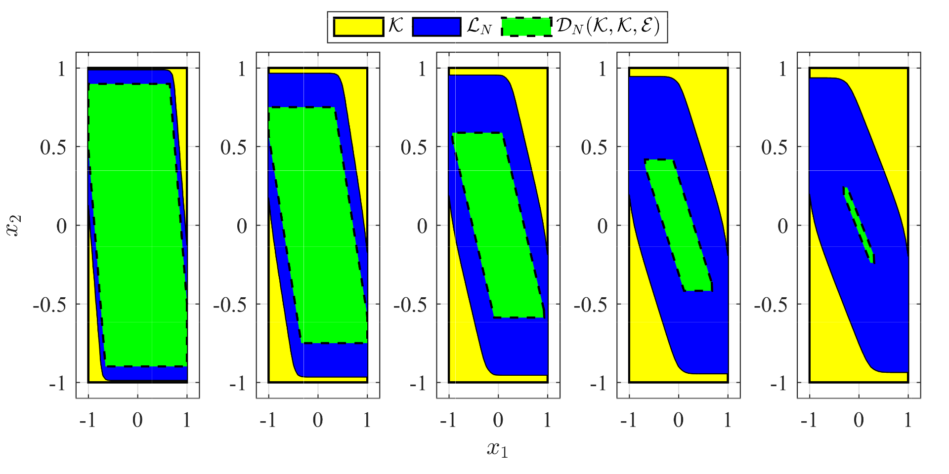
Figure 2 compares the underapproximation via Algorithm 1 and the level-sets computed using dynamic programming techniques, as in [7].The underapproximation is closest and the approximation become progressively more conservative as increases, as is expected. For , , , and hence, from Section IV-A, , indicating that .
A comparison between the total computation time for the dynamic programming method and Algorithm 1 is provided in Table I. The accuracy of dynamic programming relies on its grid size, resulting in a trade-off between accuracy and computation speed, from which Algorithm 1 does not suffer.
| Grid Size | Dynamic Programming | Algorithm 1 | Ratio |
|---|---|---|---|
| 8.16 | 0.98 | 8.3 | |
| 59.76 | 0.98 | 60.9 |
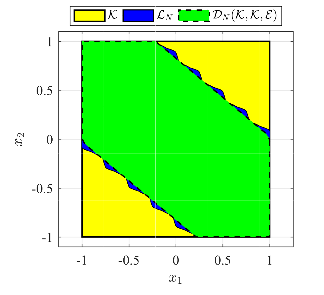
For systems with Gaussian disturbance processes that have a very low variance, the underapproximation obtained through the Lagrangian methods tightly approximates the stochastic level-set and is computed significantly faster—over times faster for a grid. Figure 3 shows a comparison of the stochastic level-set and the Lagrangian underapproximation when the Gaussian disturbance process is of the form . The bumps on the exterior of the stochastic level-set are a numerical artifact from the state-space gridding.
V-B Application to space-vehicle dynamics
In this section, we compute an underapproximation of the stochastic reach-avoid level-set for a spacecraft rendezvous docking problem using Algorithm 1. The goal is for a spacecraft, referred to as the deputy, to approach and dock to an orbiting satellite, referred to as the chief, while remaining in a predefined line-of-sight cone. The dynamics are described by the Clohessy-Wiltshire-Hill (CWH) equations [25]
| (40) |
The chief is located at the origin, the position of the deputy is at , is the orbital frequency, is the gravitational constant, and is the orbital radius of the spacecraft.
We define the state vector and input vector . We discretize the dynamics (40) in time to obtain the discrete-time LTI system,
| (41) |
where is assumed to be a Gaussian i.i.d. disturbance with , .
We define the target set and the constraint set as in [1]
| (42) | ||||
| (43) | ||||
| (44) |
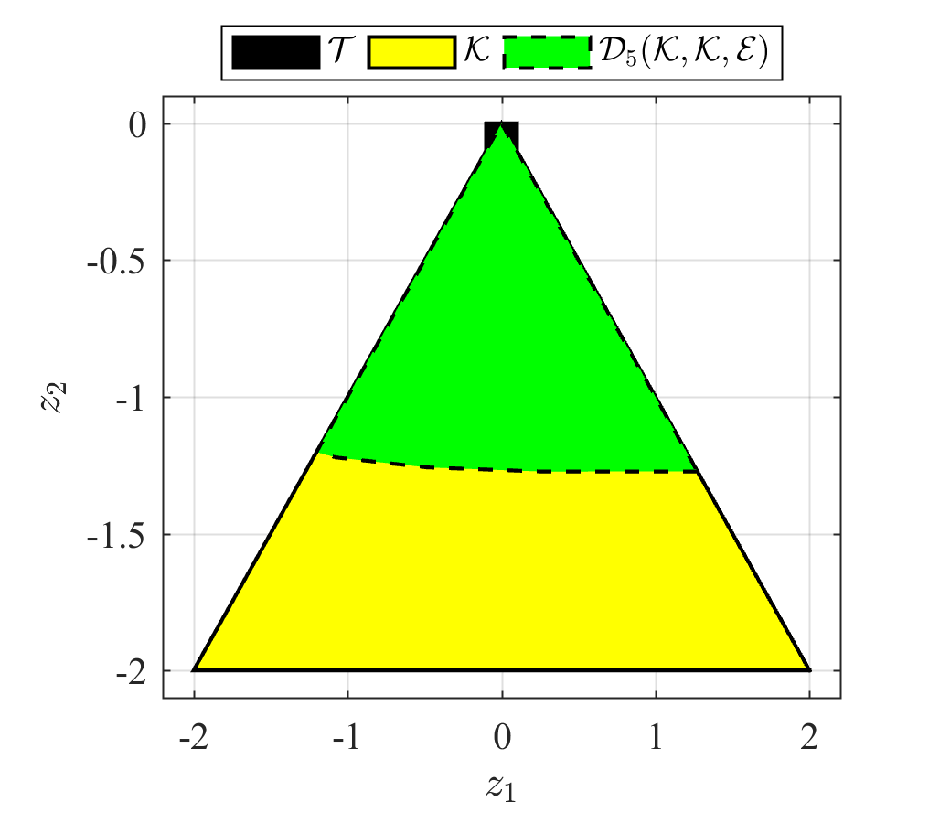
Figure 4 shows a cross-section at of the resulting underapproximation of the stochastic reach-avoid level set. The computation time for the level-set was 14.5 seconds. Because of the extreme computational requirements of solving a 4-dimensional problem via dynamic programming methods we cannot make a direct computational comparison between dynamic programming and Algorithm 1. In [1, Figure 2], a cross-section of of the stochastic reach-avoid set was approximated using convex, chance-constrained optimization and particle approximation methods. Since both of these methods require gridding, the computation time is slower, reported to be about 20 minutes, for a subset of the state space.
VI Conclusion
In this work, we provide a Lagrangian method to compute an underapproximation of a stochastic reach-avoid level-set using robust reach-avoid sets. We synthesize approaches in [4, 15] and [12, 13, 14], and characterize the sufficient conditions under which a optimal control policy for the robust reach-avoid set is also a Markov policy. We demonstrate that our Lagrangian approach to compute the underapproximation is significantly faster when compared to the dynamic programming approach. The utility of this method is problem-dependent, as the conservativeness of the underapproximations are affected by the system dynamics and noise processes.
In future, we intend to examine methods to reduce the conservativeness of the underapproximation and extend the computation of the disturbance set in Theorem 4 for disturbances other than a Gaussian random vector.
References
- [1] K. Lesser, M. Oishi, and R. S. Erwin, “Stochastic reachability for control of spacecraft relative motion,” in Proc. IEEE Conf. on Decision and Ctrl., December 2013.
- [2] C. Tomlin, I. Mitchell, A. Bayen, and M. Oishi, “Computational techniques for the verification of hybrid systems,” Proc. IEEE, vol. 91, no. 7, pp. 986–1001, 2003.
- [3] S. Summers, M. Kamgarpour, J. Lygeros, and C. Tomlin, “A stochastic reach-avoid problem with random obstacles,” in Proc. Hybrid Syst.: Comput. and Ctrl. ACM, 2011, pp. 251–260.
- [4] J. N. Maidens, S. Kaynama, I. M. Mitchell, M. M. Oishi, and G. A. Dumont, “Lagrangian methods for approximating the viability kernel in high-dimensional systems,” Automatica, vol. 49, no. 7, pp. 2017–2029, 2013.
- [5] N. Kariotoglou, D. M. Raimondo, S. Summers, and J. Lygeros, “A stochastic reachability framework for autonomous surveillance with pan-tilt-zoom cameras,” in Proc. European Ctrl. Conf., 2011, pp. 1411–1416.
- [6] G. Manganini, M. Pirotta, M. Restelli, L. Piroddi, and M. Prandini, “Policy search for the optimal control of Markov Decision Processes: A novel particle-based iterative scheme,” IEEE Trans. Cybern., pp. 1–13, 2015.
- [7] S. Summers and J. Lygeros, “Verification of discrete time stochastic hybrid systems: A stochastic reach-avoid decision problem,” Automatica, vol. 46, pp. 1951–1961, September 2010.
- [8] A. Abate, M. Prandini, J. Lygeros, and S. Sastry, “Probabilistic reachability and safety for controlled discrete time stochastic hybrid systems,” Automatica, vol. 44, pp. 2724–2734, October 2008.
- [9] A. Abate, S. Amin, M. Prandini, J. Lygeros, and S. Sastry, “Computational approaches to reachability analysis of stochastic hybrid systems,” in Proc. Hybrid Syst.: Comput. and Ctrl., 2007, pp. 4–17.
- [10] N. Kariotoglou, S. Summers, T. Summers, M. Kamgarpour, and J. Lygeros, “Approximate dynamic programming for stochastic reachability,” in Proc. European Ctrl. Conf., 2013, pp. 584–589.
- [11] N. Kariotoglou, K. Margellos, and J. Lygeros, “On the computational complexity and generalization properties of multi-stage and stage-wise coupled scenario programs,” Syst. and Ctrl. Lett., vol. 94, pp. 63–69, 2016.
- [12] D. P. Bertsekas and I. B. Rhodes, “On the minimax reachability of target sets and target tubes,” Automatica, vol. 7, no. 2, pp. 233–247, 1971.
- [13] E. C. Kerrigan, “Robust constraint satisfaction: Invariant sets and predictive control,” Ph.D. dissertation, University of Cambridge, 2001.
- [14] S. V. Raković, E. C. Kerrigan, D. Q. Mayne, and J. Lygeros, “Reachability analysis of discrete-time systems with disturbances,” IEEE Trans. Autom. Ctrl., vol. 51, no. 4, pp. 546–560, April 2006.
- [15] P. Saint-Pierre, “Approximation of the viability kernel,” Applied Mathematics and Optimization, vol. 29, no. 2, pp. 187–209, March 1994.
- [16] C. Le Geurnic, “Reachability analysis of hybrid systems with linear continuous dynamics,” Ph.D. dissertation, Université Joseph-Fourier, 2009.
- [17] M. Herceg, M. Kvasnica, C. Jones, and M. Morari, “Multi-Parametric Toolbox 3.0,” in Proc. of the European Control Conference, Zürich, Switzerland, July 17–19 2013, pp. 502–510, http://people.ee.ethz.ch/%7Empt/3/.
- [18] C. Le Guernic and A. Girard, “Reachability analysis of linear systems using support functions,” Nonlinear Analysis: Hybrid Systems, vol. 4, no. 2, pp. 250–262, 2010.
- [19] A. A. Kurzhanskiy and P. Varaiya, “Ellipsoidal toolbox,” University of California, Berkeley, Tech. Rep., 2006.
- [20] A. P. Vinod and M. M. K. Oishi, “Scalable underapproximation for stochastic reach-avoid problem for high-dimensional LTI systems using Fourier transforms,” in IEEE Control Systems Letters (L-CSS), 2017, (submitted). [Online]. Available: https://arxiv.org/abs/1703.02135
- [21] I. Kolmanovsky and E. G. Gilbert, “Theory and computation of disturbance invariant sets for discrete-time linear systems,” Mathematical Problems in Engineering, vol. 4, pp. 317–367, 1998.
- [22] D. P. Bertsekas, Dynamic Programming and Optimal Control. Vol. 1, 3rd ed. Belmont, Mass: Athena Scientific, 2005.
- [23] D. P. Bertsekas and S. E. Shreve, Stochastic Optimal Control: the Discrete Time Case. Academic Press, 1978.
- [24] P. Billingsley, Probability and Measure, 3rd ed. New York: Wiley, 1995.
- [25] W. Wiesel, Spaceflight Dynamics. New York: McGraw-Hill, 1989.