A method to measure the transverse magnetic field and
orient the rotational axis of stars

Abstract

Direct measurements of the stellar magnetic fields are based on the splitting of spectral lines into polarized Zeeman components. With few exceptions, Zeeman signatures are hidden in data noise and a number of methods have been developed to measure the average, over the visible stellar disk, of longitudinal components of the magnetic field. As to faint stars, at present observable only with low resolution spectropolarimetry, a method is based on the regression of the Stokes $V$ signal against the first derivative of Stokes $I$. Here we present an extension of this method to obtain a direct measurement of the transverse component of stellar magnetic fields by the regression of high resolution Stokes $Q$ and $U$ as a function of the second derivative of Stokes $I$. We also show that it is possible to determine the orientation in the sky of the rotation axis of a star on the basis of the periodic variability of the transverse component due to its rotation. The method is applied to data, obtained with the Catania Astrophysical Observatory Spectropolarimeter, along the rotational period of the well known magnetic star $\beta$ CrB.

1 Introduction

In stellar astrophysics, magnetic fields are measured by means of the Zeeman effect, whereby the $(2\,J+1)$-fold degeneracy of the fine structure levels of the various spectroscopic terms is completely lifted by a magnetic field. This results in the splitting of a spectral line into Zeeman components: the $\sigma_{-}$- and $\sigma_{+}$-components ($\Delta M=\pm 1$) are circularly polarized, the $\pi$-components ($\Delta M=0$) linearly. For weak to moderate fields, the displacements in wavelength of the $\sigma$-components from the unsplit line position $\lambda_{0}$ (in Å) due to a magnetic field $\vec{B}$ (in G) is given by

$$\Delta\lambda=4.67\,10^{-13}\,\bar{g}\,\lambda_{0}^{2}\,|\vec{B}|$$ (1)

where $\bar{g}$ is the so called “effective Landé factor”, related to the Landé factors $g_{1}$ and $g_{2}$ of the involved energy levels by

$$\bar{g} =0.5\,(g_{1}+g_{2})+0.25\,(g_{1}-g_{2})\,d$$ (2)

$${\rm with}~{}~{}d =[J_{1}(J_{1}+1)-J_{2}(J_{2}+1)]$$

From Eq. 1 it transpires that resolved Zeeman components can rarely be observed in optical spectra. To give an example, the $\sigma_{-}$ and the $\sigma_{+}$ components of a simple Zeeman triplet ($\bar{g}=1.0$) at $\lambda$ = 5000 Å, split in a 1 kG magnetic field, would overlap for a projected rotational velocity $v_{\rm e}\,\sin i\approx 1.5$ km s^-1 or an instrumental resolution of $R=200\,000$. In order to establish the presence of a stellar magnetic field, it rather makes sense to measure the distance between the respective centers of gravity of a spectral line in left-hand (lcp) and right-hand (rcp) circularly polarized light. The distance in wavelength between the lcp and rcp centers of gravity is proportional to the disk-averaged line-of-sight component $B_{\rm z}$ of the magnetic field vector, called “effective magnetic field” by Babcock (1947).

$$B_{||}=\frac{1}{W\cal F_{\it I_{\rm c}}}\int_{0}^{2\pi}d\phi\int_{0}^{\pi/2}B_{\rm z}\cos\theta\,\sin\theta\,d\theta\times\int[I_{\rm c}-I_{\lambda}]\,d\lambda$$ (3)

where $W$ is the equivalent width of the line, ${\cal F_{\it I_{\rm c}}}$ denotes the continuum flux at the wavelength of the line; $\phi$ and $\theta$ are polar coordinates. $I_{\rm c}$ and $I_{\lambda}$ represent the respective continuum and line intensities at the coordinate ($\theta$, $\phi$). $B_{||}$ is commonly obtained from the relation given by Mathys (1994):

$$R_{V}^{(1)}=\frac{1}{W}\int{\frac{V_{c}-V_{\lambda}}{I_{c}}\,(\lambda-\lambda_{0})\,d\lambda}=4.67\,10^{-13}\,\bar{g}\,\lambda_{0}^{2}\,B_{||}$$ (4)

It is a fact that with increasing instrumental smearing, Stokes polarization profiles rapidly become unobservable (Leone & Catanzaro, 2001; Leone et al., 2003); on the other hand, high resolution spectropolarimetry is at present limited to bright (V$\lesssim 10$) stars. To overcome these limitations, Angel & Landstreet (1970) introduced a method based on narrow-band ($\sim$ 30 Å) circular photopolarimetry in the wings of Balmer lines for the measurement of magnetic fields of stars that could not be observed with high-resolution spectropolarimetry. The difference between the opposite circularly polarized photometric intensities is converted to a wavelength shift and subsequently to the effective longitudinal field ${\rm{B_{||}}}$. Another method, suggested by Bagnulo et al. (2002b), is based on the relation between Stokes $V$ and $I$ for spectral lines whose intrinsic width is larger than the magnetic splitting (Mathys, 1989):

$$\frac{V_{\lambda}}{I_{\lambda}}=-4.67\,10^{-13}\,\bar{g}\,\lambda^{2}\,B_{||}\,\frac{1}{I_{\lambda}}\,\frac{\partial I_{\lambda}}{\partial\lambda}$$ (5)

This linear fitting of Stokes $V$ against the gradient of Stokes $I$ (Eq. 5) to measure the effective magnetic field of faint targets on the basis of low resolution spectropolarimetry without wasting any circular polarized signal has opened a new window. A method to measure the magnetic fields of previously inscrutable objects has indeed been largely used. The reader can refer to Bagnulo et al. (2015) for a review on this method and its results.

The problem of measuring the magnetic field of faint stars represents a special case of the more general problem of how to recover Stokes profiles “hidden” in photon noise. With reference to the very weak magnetic fields of late-type stars, the solution introduced by a lamented colleague and friend, Meir Semel, consisted in adding the Stokes $V$ profiles of all lines present in a spectrum, obtaining a pseudo profile of a very high signal to noise (S/N) ratio (Semel & Li, 1996). This idea has been further developed by Donati et al. (1997) who introduced the Least Squares Deconvolution (LSD) method. Later, Semel et al. (2006) initiated yet another approach to the add-up of Stokes profiles from noisy spectra, based on Principal Component Analysis.

The measurement of the $B_{||}$ component is important to assign a lower limit to the strength of a magnetic field. But in order to constrain the magnetic topology, the transverse component $B_{\bot}$ is necessary too. To our knowledge, no direct measurements of the transverse component of a stellar magnetic field have yet been obtained. No relations similar to Eqs. 4 and 5 have yet been implemented. According to Landi Degl’Innocenti & Landolfi (2004), Stokes $Q$ and $U$ are related to the second derivative of Stokes $I$ by

$$\frac{Q_{\lambda}}{I_{\lambda}}= -5.45\,10^{-26}\,\bar{G}\,\lambda^{4}\,B_{\bot}^{2}\,\cos\,2\chi\,\frac{1}{I_{\lambda}}\,\frac{\partial^{2}I}{\partial\lambda^{2}}$$ (6)

$$\frac{U_{\lambda}}{I_{\lambda}}= -5.45\,10^{-26}\,\bar{G}\,\lambda^{4}\,B_{\bot}^{2}\,\sin\,2\chi\,\frac{1}{I_{\lambda}}\,\frac{\partial^{2}I}{\partial\lambda^{2}}$$ (7)

where

$$\bar{G}=\bar{g}^{2}-\delta$$ (8)

is the second order effective Landé factor, with

$$\delta =(g_{1}-g_{2})^{2}\,(16s-7d^{2}-4)/80$$

$$s =[J_{1}(J_{1}+1)+J_{2}(J_{2}+1)]$$

and $J_{1}$ and $J_{2}$ the angular momenta of the involved energy levels.

Stokes $Q$ and $U$ signals across the line profiles are weaker than the $V$ signal and instrumental smearing is more destructive for Stokes $Q$ and $U$ profiles than for Stokes $V$ (Leone et al., 2003) because their variations are more complex and occur on shorter wavelength scales. As a result, Stokes $Q$ and $U$ have rarely been detected – being hidden in the noise even in stars characterized by very strong Stokes $V$ signals – but it is worth mentioning that Wade et al. (2000) have successfully applied the LSD method also to Stokes $Q$ and $U$ profiles. When observed, Stokes $Q$ and $U$ profiles represent a strong constraint to the magnetic geometry (Bagnulo et al., 2001). Following Landi Degl’Innocenti et al. (1981) who showed that broadband linear polarization arises from saturation effects in spectral lines formed in a magnetic field (Calamai et al., 1975), Bagnulo et al. (1995) have used phase-resolved broadband linear photopolarimetry to constrain stellar magnetic geometries.

In Section 3, we show that application of the linear regression method to high resolution Stokes $V$ spectra results in highly accurate measurements of the stellar effective magnetic field (hereafter longitudinal field). An extension of this regression method to high resolution Stokes $Q$ and $U$ spectra on the other hand results in a direct measure of the mean transverse component of the field (hereafter transverse field). For this purpose, we have obtained a series of full Stokes $IQUV$ spectra of $\beta$ CrB (Section 2) over its rotational period with the Catania Astrophysical Observatory Spectropolarimeter (Leone et al., 2016).

In Section 4.2, we will show that, as a consequence of the stellar rotation, the transverse component of the magnetic field describes a closed loop in the sky, offering the possibility to determine the orientation of the rotational axis.

Figure 1: Observed Stokes $I,Q,U$ and $V$ spectra of the magnetic star $\beta$ CrB at rotational phase $\phi=0.66$ (top block of six panels) and $\phi=0.85$ (bottom block of six panels). Phase values are computed according to the ephemeris (10). Also plotted are Stokes $Q$ and $U$ as a function of the second derivative of Stokes $I$, and Stokes $V$ as a function of the first derivative of Stokes $I$. Noise spectra (Eq. 11) are shown to quantify the photon and extraction errors. Noise constant with wavelength validates the correctness of the data reduction. Slope with errors are reported.

2 $\beta$ CrB observations and data reduction

Ever since Babcock (1949b), $\beta$ CrB has been one of the most studied magnetic chemically peculiar main sequence star. Distinctive characteristics of this class of stars are a) a very strong magnetic field as inferred from the integrated Zeeman effect. Typical fields are 1 - 10 kG, the strongest known reaching $35$ kG; b) Variability of the magnetic field, spectral lines and luminosity with the same period; the longitudinal magnetic field often reverses its sign. So far, the oblique rotator is the only model that provides an acceptable interpretation of the above-mentioned phenomena (Babcock, 1949a; Stibbs, 1950). It is essentially based on two hypotheses: 1) The magnetic field is largely dipolar with the dipole axis inclined with respect to the the rotational axis, and 2) Over- and under-abundances of chemical elements are distributed non-homogeneously over the stellar surface. All observed variations are a direct consequence of stellar rotation.

For comparison with results on $\beta$ CrB found in the literature we adopted the measurements of the longitudinal field by Mathys (1994), the measurements of the “surface” field (the integrated field modulus)

$$B_{s}=\frac{1}{W\cal F_{\it I_{\rm c}}}\int_{0}^{2\pi}d\phi\int_{0}^{\pi/2}|B|\cos\theta\,\sin\theta\,d\theta\times\int[I_{\rm c}-I_{\lambda}]d\lambda$$ (9)

by Mathys et al. (1997) and the ephemeris by Bagnulo et al. (2001):

$$JD(B_{||}^{\rm max})=2\,443\,310.221+18.4868\hskip 28.45274pt\rm days$$ (10)

The linear polarization of $\beta$ CrB has been measured 32 times over its rotational period. These data have been obtained with the Catania Astrophysical Observatory Spectropolarimeter (CAOS) from June to July 2014 in the 370-860 nm range with resolution R = 55 000 (Leone et al., 2016), the minimum signal-to-noise ratio was S/N = 400. With respect to the acceptance axis of the polarizer, we obtained Stokes $V$ by setting the fast axis of the quarter wave-plate retarder to $\alpha=+45\arcdeg$ and $-45\arcdeg$ respectively. The fast axis of the half wave-plate retarder has been rotated by $\alpha=0\arcdeg$ and $45\arcdeg$ to measure Stokes $Q$, and by $\alpha=22.5\arcdeg$ and $67.5\arcdeg$ to measure Stokes $U$.

There are several methods to measure the degree of polarization from o-rdinary and e-xtraordinary beams from the polarizer. As to the dual beam spectropolarimetry, the ratio method was introduced by Tinbergen & Rutten (1992). It is assumed that there is a time independent (instrumental) sensitivity $G$, for example due to pixel-by-pixel efficiency variations – together with a time dependent sensitivity $F$ of spectra – for example due to variations in the transparency of the sky. So a photon noise dominated Stokes parameter (generically $P=V,Q$ or $U$) can be obtained from the recorded o-rdinary and e-xtraordinary spectra, $S_{\alpha,o}$ and $S_{\alpha,e}$ respectively, at rotations $\alpha_{1}$ and $\alpha_{2}$ by:

$$S_{\alpha_{1},o} =0.5\,(I+P)\,G_{o}F_{\alpha_{1}} S_{\alpha_{1},e} =0.5\,(I-P)\,G_{e}F_{\alpha_{1}}$$

$$S_{\alpha_{2},o} =0.5\,(I-P)\,G_{o}F_{\alpha_{2}} S_{\alpha_{2},e} =0.5\,(I+P)\,G_{e}F_{\alpha_{2}}$$

Hence:

$$\frac{P}{I}=\frac{R_{P}-1}{R_{P}+1}\hskip 42.67912pt{\rm with}\hskip 10.81218ptR_{P}^{2}=\frac{S_{\alpha_{1},o}/S_{\alpha_{1},e}}{S_{\alpha_{2},o}/S_{\alpha_{2},e}}$$

In addition we compute the noise polarization spectrum:

$$\frac{N}{I}=\frac{R_{N}-1}{R_{N}+1}\hskip 42.67912pt{\rm with}\hskip 10.81218ptR_{N}^{2}=\frac{S_{\alpha_{1},o}/S_{\alpha_{2},e}}{S_{\alpha_{2},o}/S_{\alpha_{1},e}}$$ (11)

to check any possible error in Stokes $P/I$. Without errors, the noise polarization spectrum is expected to present no dependence on the Stokes $I$ derivatives (Leone, 2007; Leone et al., 2011).

The preferred use of Eqs. 5, 6 and 7 over the original relations given by Landi Degl’Innocenti & Landolfi (2004) is due to the higher accuracy that can be achieved in measuring $Q/I,U/I$ and $V/I$ as compared to $Q,U$ and $V$.

3 Measuring magnetic field components

As stated in the introduction, the linear fitting of Stokes $V$ versus the first derivative of Stokes $I$ of Balmer line profiles has opened a new way to measure $B_{||}$ of stars on the basis of low resolution spectra. Introducing this method, Bagnulo et al. (2002b) quoted a series of papers based on photopolarimetry of Balmer line wings to justify the validity of Eq. 5 also for the whole visible disk of a star with a complex magnetic field and despite the limb darkening (Mathys et al., 2000).

Martínez González & Asensio Ramos (2012) have shown that Eqs. 5, 6 and 7 are valid for disk-integrated line profiles of rotating stars with a magnetic dipolar field, provided the rotational velocity is not larger than eight times the Doppler width of the local absorption profiles. We have performed numerical tests with Cossam (Stift et al., 2012) to find out how far the derivative of the Stokes $I$ profile reflects Zeeman broadening before being dominated by the rotational broadening. As a limiting case, we have assumed the dipole axis orthogonal to the rotation axis, both being tangent to the celestial sphere. Two cases are shown in Figure 2 and results are summarized in Table 1 for the spectral resolution of CAOS.

Figure 2: Examples of Cossam simulations for a magnetic dipole, B_p = 10 kG, orthogonal to the rotational axis and along the E-W direction. Left panel: star rotating at 3 km s^-1, right panel: 18 km s^-1.

Table 1: Ratio between the measured transverse field and the expected value, derived by applying the derivative method. In this particular case the equatorial velocity is equal to the projected velocity.

		veq [km s-1]
		0	3	6	12	18
Bp[G]	10	1.93	1.18	1.17	0.79	3.51
	100	0.96	1.13	1.13	1.13	3.37
	1000	0.93	1.06	1.08	1.15	3.32
	10000	0.81	0.84	1.02	1.07	1.21

These numerical simulations show that by applying the slope method, the transverse field of a star observed with CAOS is estimated correctly to within 20% for rotational velocities up to 12 km s^-1. We ascribe the anomalous value for a non-rotating star with a weak (10 G polar) field to the fact that the spectral line profiles are dominated by the 5.5 km s^-1 instrumental smearing.

We have also addressed the capability to measure the transverse component of fields that are not purely dipolar. As a benchmark, we have extended the previous numerical tests with Cossam for a star rotating at 3 km s^-1 and B_p = 10 kG. The dipole, whose axis is still going through the center of the star, has been displaced in the direction of the positive pole. As a function of the decentering in units of the stellar radius $a$, the ratio between the mesured transverse field and the expected value is $r(a=0.0)=0.84$, $r(a=0.1)=1.06$, $r(a=0.2)=1.16$, $r(a=0.3)=1.15$, and $r(a=0.4)=4.57$

It appears therefore legitimate to apply the method to our spectra of $\beta$ CrB, which displays a rotational velocity of 3 km s^-1 (Ryabchikova et al., 2004).

3.1 The longitudinal field component of $\beta$ CrB

We have applied the method to our high resolution spectra and found a very high precision of the measurements. Figure 1 shows Stokes $I$ and $V$ of $\beta$ CrB at rotational phases $\phi=0.66$ and 0.85 in a 30 Å  interval centered on the Fe ii 5018.44 Å line. Figure 1 also shows Stokes $V$ as a function of the first derivative of Stokes $I$ and its linear fit. If $\bar{g}$ = 1, the slope gives an error in the measured $B_{||}$ of about 40 G. It is worthwhile noting that the same procedure, as applied to the noise spectra, gives a much smaller error of less than 4 G. We ascribe the 40 G error to the line-by-line differences in the $\bar{g}$ Landé factors, resulting in the superposition of straight lines with different slopes. The observed Stokes $I$ and $V$ profiles of a generic spectral line $k$, with effective Landé factor $g^{k}_{\rm eff}$, define a straight line in the $-4.67\times 10^{-13}\lambda^{2}\frac{1}{I_{\lambda}}\frac{\partial I_{\lambda}}{\partial\lambda}$ vs $\frac{V_{\lambda}}{I_{\lambda}}$ plane whose slope is $c_{k}=g^{k}_{\rm eff}B_{||}$. Using a set of $N$ spectral lines we measure an average value for the longitudinal field $<B_{||}>=\frac{\sum c_{k}}{N}=<g_{\rm eff}>B_{||}$. The relative error in the longitudinal field measure is given by the dispersion of the effective Landé factors.

Even though the precision is very high, the accuracy of the longitudinal field measurements depends on the adopted $\bar{g}$ value; usually this is assumed equal to unity. In Leone (2007), we have numerically shown that the average value of the Landé factors of the spectral lines of the magnetic star $\gamma$Equ, observed in the 3780-4480 Å interval and weighted by their intensity, is about 1.1. As to $\beta$ CrB, adopting the effective temperature, gravity and abundances given by Ryabchikova et al. (2004), we have extracted from VALD the list of expected spectral lines and found an average value of $\bar{g}=1.2\pm 0.4$. We conclude that the linear regression method measures the longitudinal field of a star with a precision equal to the standard distribution of the effective Landé factors of the spectral lines involved.

3.2 The transverse field component

As an extension to the method described above to measure the longitudinal field, we have plotted the Stokes $Q$ and $U$ signals as a function of the second derivative of Stokes $I$ (Eqs. 6 and 7). Figure 1 shows the expected linear dependencies for $\beta$ CrB at two different rotational phases.

The conversion of the slopes to transverse field measures is less straightforward than in the longitudinal case. Line-by-line differences in the second order Landé factors are larger than differences in the effective Landé factors (Eq. 2). The second order Landé factors can become negative (Eq. 8), effective Landé factors only very exceptionally. In a list of solar Fe i lines given by Landi Degl’Innocenti & Landolfi (2004) some 8% of $\bar{G}$ values are negative.

Table 2 reports the transverse field of $\beta$ CrB by applying Eqs. 6 and 7 to 50 Å blocks of CAOS spectra in the 5000 to 6000 Å interval. As for $\bar{g}$, the adopted $\bar{G}$ of a block represents the average of the $G$ value of the predicted spectral lines. In order to check the reliability of our quantitative measurements of the transverse field, we have applied the method also to the Fe ii 5018.44 Å  line which presents well defined Stokes profiles and is among the lines selected for solar studies in the Télescope Héliographique pour l’Etude du Magnétisme et des Instabilités Solaires (THEMIS).

As applied to our collected spectra and on the basis of the ephemeris given in Eq. 10, $\beta$ CrB presents a transverse field that varies with the rotation period (Figure 3). The average value is about 1 kG and the amplitude as large as 0.25 kG. A comparison (Table 2) with results from the Fe ii 5018.44 Å  line reveals general agreement; however the associated errors are larger. We suppose that the error in measuring the transverse field – i.e. the slope error – is dominated by the scatter in the second order Landé factors, similar to what we found for the longitudinal field.

The angle $\chi$ is variable too with the rotation period, see Figure 3. Since by definition, $\chi$ is limited to the range $0-180\arcdeg$, it exhibits a saw-tooth behavior.

Table 2: Measured transverse magnetic field of $\beta$ CrB. Eqs. 6 and 7 have been applied to CAOS spectra in the range 5000 to 6000 Å  and to a well known single iron line.

	5000 - 6000 Å		Feii 5018.44 Å
HJD	$B_{\bot}\pm\sigma$	$\chi\pm\sigma$	$B_{\bot}\pm\sigma$	$\chi\pm\sigma$
2450000	kG	°	kG	°
6787.511	1.117$\pm$0.084	85$\pm$ 5	0.930$\pm$0.012	88$\pm$ 1
6788.560	0.923$\pm$0.160	69$\pm$ 5	0.877$\pm$0.015	70$\pm$20
6799.481	0.907$\pm$0.223	48$\pm$12	0.841$\pm$0.015	45$\pm$43
6802.471	0.737$\pm$0.123	147$\pm$11	0.564$\pm$0.025	148$\pm$31
6807.515	1.109$\pm$0.162	63$\pm$ 6	0.897$\pm$0.019	63$\pm$27
6809.448	1.138$\pm$0.167	34$\pm$ 5	0.982$\pm$0.016	37$\pm$35
6815.452	1.217$\pm$0.147	106$\pm$ 6	11207$\pm$0.019	101$\pm$13
6816.436	1.005$\pm$0.149	89$\pm$ 8	0.995$\pm$0.015	84$\pm$ 5
6820.484	0.849$\pm$0.082	22$\pm$16	0.794$\pm$0.021	12$\pm$ 9
6822.429	0.735$\pm$0.108	117$\pm$11	0.608$\pm$0.022	127$\pm$40
6826.417	1.073$\pm$0.122	55$\pm$ 3	0.960$\pm$0.014	55$\pm$36
6829.409	1.155$\pm$0.153	3$\pm$ 4	1.010$\pm$0.013	1$\pm$ 1
6830.474	1.237$\pm$0.155	161$\pm$ 6	1.094$\pm$0.015	160$\pm$20
6831.422	1.311$\pm$0.124	144$\pm$ 5	1.152$\pm$0.013	143$\pm$37
6833.478	1.289$\pm$0.129	108$\pm$ 6	1.134$\pm$0.020	108$\pm$20
6835.405	1.000$\pm$0.098	81$\pm$ 7	0.949$\pm$0.019	75$\pm$14
6836.408	0.873$\pm$0.180	51$\pm$24	0.703$\pm$0.019	44$\pm$41
6844.369	1.246$\pm$0.136	60$\pm$ 3	1.030$\pm$0.014	60$\pm$30
6848.338	1.139$\pm$0.134	171$\pm$17	1.000$\pm$0.014	173$\pm$ 7
6849.343	1.004$\pm$0.094	152$\pm$ 5	0.976$\pm$0.021	150$\pm$29
7129.556	1.144$\pm$0.142	103$\pm$ 9	1.129$\pm$0.014	96$\pm$ 7
7189.467	0.798$\pm$0.130	15$\pm$20	0.691$\pm$0.017	5$\pm$ 3
7190.426	0.766$\pm$0.128	163$\pm$ 6	0.733$\pm$0.020	169$\pm$12
7191.416	0.619$\pm$0.102	118$\pm$17	0.483$\pm$0.024	135$\pm$41
7193.425	0.757$\pm$0.112	90$\pm$ 9	0.657$\pm$0.018	93$\pm$ 7

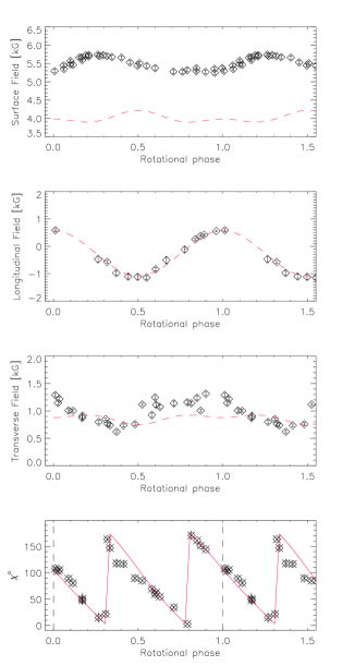
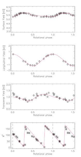
Figure 3: Longitudinal and transverse magnetic field of $\beta$ CrB as well as the angle $\chi$ of the transverse component with respect to the North-South meridian (measured counterclockwise) are plotted as a function of the rotational phase. The left panels show the expected variations for a dipole, whereas the right panels pertain to a field resulting from the superposition of a dipole, a quadrupole and an octupole. The vertical line marks the positive extremum of the longitudinal field, i.e. the rotational phase when the line of sight, the rotation axis and the dipole axis all lie in the same plane. At this phase, the transverse field is also aligned with the rotation axis; the angle $\chi$ gives the orientation of the rotation axis with respect to the North-South direction in the sky.

4 The added-value of the transverse field

Large efforts have gone into the study of stellar magnetic fields (Mestel, 1999) but it is still not possible to predict the magnetic field geometry of an ApBp star. As mentioned in the introduction, the magnetic variability of early-type upper main sequence stars is thought to be due to a mainly dipolar field, with the dipole axis inclined with respect to the rotational axis. Once the mean field modulus could be determined in addition to the longitudinal field it became clear that the magnetic configurations went beyond simple dipoles (Preston, 1967). Deutsch (1970) was the first to model the field with a series of spherical harmonics, Landstreet (1970) introduced the decentred dipole, Landstreet & Mathys (2000) adopted a field characterized by a co-linear dipole, quadrupole and octupole geometry and Bagnulo et al. (2002a) modeled the field by a superposition of a dipole and a quadrupole field, arbitrarily oriented.

It has been known for quite some time that the surface field of $\beta$ CrB cannot be represented by a simple dipole (Wolff & Wolff, 1970). Let us however, for the present purpose, look at the variability of the longitudinal field within the framework of a pure dipole (Stibbs, 1950)

$$B^{d}_{||}(t)=\frac{15+u}{15-5u}\frac{B_{d}}{4}\left(\cos i\cos\beta_{d}+\sin i\sin\beta_{d}\cos\frac{2\pi}{P}\right)$$ (12)

– where $u$ is the limb coefficient, $i$ the angle between the line of sight and the rotation axis, $\beta_{d}$ the angle between dipole and rotation axes, $B_{d}$ the magnetic field strength at the poles and $P$ the rotation period. Hence, the Schwarzschild (1950) relation

$$B^{d}_{||}(min,max)=\frac{15+u}{15-5u}\frac{B_{d}}{4}\cos(\beta_{d}\pm i)$$ (13)

and Preston (1971) relation

$$\tan i\,\tan\beta_{d}=\frac{1-r_{||}}{1+r_{||}}$$ (14)

– where $r_{||}$ is the ratio between minimum and maximum longitudinal field values – one can establish combinations of $i$, $\beta_{d}$ and $B_{d}$ which match an observed sinusoidal $B_{||}$ variability. We note that the combination $i=153\arcdeg$, $\beta_{d}=81\arcdeg$ and $B_{d}=6.2$ kG yields the observed average value of the transverse field, however underestimating the surface field (left panel of Figure 3). On the other hand, adopting $i=161\arcdeg$, $\beta_{d}=84\arcdeg$ and $B_{d}=8.6$ kG, we obtain a match for the average field modulus, but now the transverse field is overestimated.

In order to correctly predict the observed variability of longitudinal, transverse and surface field of $\beta$ CrB, it is obviously necessary to assume a magnetic field geometry without cylindrical symmetry (Mathys, 1993). We have thus decided to model the magnetic variability by taking a dipole, a quadrupole and an octupole with symmetry axes pointing in different directions with respect to the rotation axis and with respect to each other. As the reference plane we adopt the plane defined by the rotation axis and the line of sight; the rotation phase $\phi$ is zero when the dipole axis lies in this plane. The right panel of Figure 3 shows the result of our best fit with $i=153\arcdeg$,
$B_{d}=\,\,+6.1$ kG,  $\beta_{d}=86\arcdeg$,
$B_{q}=\,\,+3.9$ kG,  $\beta_{q}=88\arcdeg$,  $\phi_{q}=64\arcdeg$,
$B_{o}=-10.7$ kG,  $\beta_{o}=20\arcdeg$,  $\phi_{o}=40\arcdeg$.
$\phi_{q}$ and $\phi_{o}$ represent the azimuth of quadrupole and octupole respectively.

The problem of the uniqueness of this particular magnetic configuration is outside the scope of this paper. At present we focus exclusively on the added value of knowing the transverse component in relation to the orientation of the rotational axis, the radius and the equatorial velocity of magnetic stars.

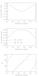
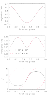
Figure 4: Two examples of magnetic dipoles indistinguishable from the respective longitudinal field variations that present very different $\chi$ variations. Field values are given in units of the polar strength.

4.1 Degeneracy between $i$ and $\beta_{d}$

Fig. 3 shows that the angle $\chi$ is dominated by the dipolar component with only a negligible dependence on the higher order components of the magnetic field. This doesn’t really come as a surprise: Schwarzschild (1950) has shown that the maximum value of the longitudinal field is equal to $\sim\,$30% of the polar value for a dipole and equal to $\sim$ 5% for a quadrupole. Numerical integration over the visible stellar disk shows that the same holds true for the transverse field: $B_{||}^{max}=B_{\perp}^{max}\,\sim 0.30\,B_{d}\sim 0.05\,B_{q}\sim 0.02\,B_{o}$, considering also the octupole. This is an intuitive result since the longitudinal field for an observer simply is the transverse field of another observer located at 90°. For example, the longitudinal component as measured by an observer located above the north pole of a dipole is the transverse component for an observer lying in the magnetic equator. The latter can see half of the southern hemisphere that presents exactly the magnetic field configuration of the invisible half of the north hemisphere.

It is straight to show that the previous relations 12, 13 and 14 together with an equal set of relations where $i$ is replaced by $i+90\arcdeg$, that are valid for the transverse field, break the degeneracy between $i$ and $\beta_{d}$. We conclude that the knowledge of the transverse field component removes the indeterminacy in the Schwarzschild relation (Eq. 13) between the angles formed by the rotation axis with the line-of-sight ($i$) and the magnetic axis ($\beta$).

We note that it is not necessary to solve these equations to solve the degeneracy between $i$ and $\beta_{d}$ when the $\chi$ variation with the stellar rotation is available. It happens that, if $i$ is larger than $\beta_{d}$ the $\chi$ variation is not a sawtooth (Figure 4).

4.2 Orientation of the stellar rotational axis

The longitudinal and transverse components of a dipolar field are projected along the dipole axis. This, within the framework of the oblique rotator model, describes a cone around the rotation pole. It happens that when we observe the extrema of the longitudinal field, the transverse field is projected onto the rotation axis. This means that, when we observe the extrema of the longitudinal field, the measured angle $\chi$ represents the angle between the rotation axis and the North-South direction in the sky. This simple consideration gives us the possibility to determine the absolute orientation of the rotation axis of a star hosting a dominant dipolar magnetic field. From our data we conclude that the rotation axis of $\beta$ CrB is tilted by about 110$\arcdeg$ with respect to the N-S direction.

4.3 Equatorial velocity and Stellar radius

Once the degeneracy between $i$ and $\beta_{d}$ removed, the stellar radius can be inferred from the relation valid for a rigid spherical rotator

$$\rm v_{\rm e}\,\sin i[km\,s^{-1}]\,P[days]=50.6\,\,R[R_{\odot}]\sin i$$ (15)

where $P$ is the rotational period. As to $\beta$ CrB, Kurtz et al. (2007) report a $\rm v_{\rm e}\,\sin i$ in the range $3.0-3.8$ km s^-1. The indeterminacy ($i=153\arcdeg,\beta_{d}=81\arcdeg$) or ($i=81\arcdeg,\beta_{d}=153\arcdeg$) from the Schwarzschild relation would thus result in the following values of the stellar radius: $1.25\pm 0.15\,R_{\odot}$ or $2.75\pm 0.30\,R_{\odot}$. Our determination of the angle $i=153\arcdeg$ (implying $2.75\,R_{\odot}$) agrees with the interferometric value of $2.6\,R_{\odot}$ for the radius of $\beta$ CrB obtained by Bruntt et al. (2010). The equatorial velocity lies between 6.6 and 8.4 km s^-1.

5 Conclusions

The linear regression between Stokes $V$ and the first derivative of Stokes $I$ in low resolution spectroscopy was introduced by Bagnulo et al. (2002b) as a method for estimating the longitudinal magnetic fields of faint stars.

We have carried out phase-resolved and high-resolution full Stokes spectropolarimetry of the magnetic chemically peculiar star $\beta$ CrB with the Catania Astrophysical Observatory Spectropolarimeter (Leone et al., 2016). On the basis of these data, we have shown that it is possible to extend the previous method to the high resolution spectropolarimetry with the more general aim of recovering the Stokes profiles hidden in the photon noise. A condition of faint stars as observed at low resolution but also of very weak stellar magnetic fields. The precision appears to be limited by our knowledge of Landé factors and by the non homogeneous distribution of chemical elements on the visible disk. Leone & Catanzaro (2004) found that measuring the longitudinal field, element by element, different values are obtained monitoring the equivalent width variations with the rotation period of HD 24712.

We have also shown that a regression of Stokes $Q$ and $U$ with respect to the second derivative of Stokes $I$ provides a direct measure of the transverse component of a stellar magnetic field and its orientation in the sky. If the magnetic field is not symmetric with respect to the rotation axis, the transverse field vector rotates in the sky. Having found that the dipolar component of the field is mainly responsible for the transverse component, we conclude that it is possible to determine the orientation of the rotation axis with respect to the sky: the value of the angle between the rotation axis and the North-South direction corresponds to the value of $\chi$ at the rotational phase where the longitudinal field reaches an extremum, viz. $\Theta=\chi(B_{||}^{extrem.})$

To our knowledge, the transverse component has never before been measured directly. The interpretation of broadband linear photopolarimetry by Landi Degl’Innocenti et al. (1981), based on the linear polarization properties of spectral lines formed in the presence of a magnetic field and its application to phase-resolved data by Bagnulo et al. (1995) to constrain the magnetic field geometries of chemically peculiar stars represent an approach somewhat similar to ours. It is worthwhile noting that $\beta$ CrB has been modeled from phase-resolved broadband linear photopolarimetry by Leroy et al. (1995) and by Bagnulo et al. (2000) who found $\Theta=135\arcdeg$ and $\Theta=124\arcdeg$ respectively. These values have to be compared with our result of $\Theta=110\arcdeg$.

In view of the improving capability to obtain high resolution spatial observations via optical and radio interferometry, it becomes increasingly important to know the orientation of the rotation axis in the sky. The determination of the transverse field is thus fundamental in multi-parametric problems such as the 3D mapping of the magnetospheres of early-type radio stars (Trigilio et al., 2004; Leone et al., 2010; Trigilio et al., 2011).

References

- Angel & Landstreet (1970) Angel, J. R. P., & Landstreet, J. D. 1970, ApJ, 160, L147
- Babcock (1947) Babcock, H. W. 1947, ApJ, 105, 105
- Babcock (1949a) —. 1949a, ApJ, 110, 126
- Babcock (1949b) —. 1949b, The Observatory, 69, 191
- Bagnulo et al. (2015) Bagnulo, S., Fossati, L., Landstreet, J. D., & Izzo, C. 2015, A&A, 583, A115
- Bagnulo et al. (1995) Bagnulo, S., Landi Degl’Innocenti, E., Landolfi, M., & Leroy, J. L. 1995, A&A, 295, 459
- Bagnulo et al. (2002a) Bagnulo, S., Landi Degl’Innocenti, M., Landolfi, M., & Mathys, G. 2002a, A&A, 394, 1023
- Bagnulo et al. (2000) Bagnulo, S., Landolfi, M., Mathys, G., & Landi Degl’Innocenti, M. 2000, A&A, 358, 929
- Bagnulo et al. (2002b) Bagnulo, S., Szeifert, T., Wade, G. A., Landstreet, J. D., & Mathys, G. 2002b, A&A, 389, 191
- Bagnulo et al. (2001) Bagnulo, S., Wade, G. A., Donati, J.-F., et al. 2001, A&A, 369, 889
- Bruntt et al. (2010) Bruntt, H., Kervella, P., Mérand, A., et al. 2010, A&A, 512, A55
- Calamai et al. (1975) Calamai, G., Landi Degl’Innocenti, E., & Landi Degl’Innocenti, M. 1975, A&A, 45, 297
- Catalano et al. (1993) Catalano, F. A., Renson, P., & Leone, F. 1993, A&AS, 98, 269
- Deutsch (1970) Deutsch, A. J. 1970, ApJ, 159, 985
- Donati et al. (1997) Donati, J.-F., Semel, M., Carter, B. D., Rees, D. E., & Collier Cameron, A. 1997, MNRAS, 291, 658
- Kurtz et al. (2007) Kurtz, D. W., Elkin, V. G., & Mathys, G. 2007, MNRAS, 380, 741
- Landi Degl’Innocenti & Landolfi (2004) Landi Degl’Innocenti, E., & Landolfi, M. 2004, Astrophysics and Space Science Library, Vol. 307, Polarization in Spectral Lines, doi:10.1007/978-1-4020-2415-3
- Landi Degl’Innocenti et al. (1981) Landi Degl’Innocenti, M., Calamai, G., Landi Degl’Innocenti, E., & Patriarchi, P. 1981, ApJ, 249, 228
- Landstreet (1970) Landstreet, J. D. 1970, ApJ, 159, 1001
- Landstreet & Mathys (2000) Landstreet, J. D., & Mathys, G. 2000, A&A, 359, 213
- Leone (2007) Leone, F. 2007, MNRAS, 382, 1690
- Leone et al. (2010) Leone, F., Bohlender, D. A., Bolton, C. T., et al. 2010, MNRAS, 401, 2739
- Leone et al. (2003) Leone, F., Bruno, P., Cali, A., et al. 2003, in Proc. SPIE, Vol. 4843, Polarimetry in Astronomy, ed. S. Fineschi, 465
- Leone & Catanzaro (2001) Leone, F., & Catanzaro, G. 2001, A&A, 365, 118
- Leone & Catanzaro (2004) —. 2004, A&A, 425, 271
- Leone et al. (2011) Leone, F., Martínez González, M. J., Corradi, R. L. M., Privitera, G., & Manso Sainz, R. 2011, ApJ, 731, L33
- Leone et al. (2016) Leone, F., Avila, G., Bellassai, G., et al. 2016, AJ, 151, 116
- Leroy et al. (1995) Leroy, J. L., Landolfi, M., Landi Degl’Innocenti, M., et al. 1995, A&A, 301, 797