DYNAMIC TRANSITION IN SYMBIOTIC EVOLUTION INDUCED BY GROWTH RATE VARIATION

Abstract

In a standard bifurcation of a dynamical system, the stationary points (or more generally attractors) change qualitatively when varying a control parameter. Here we describe a novel unusual effect, when the change of a parameter, e.g. a growth rate, does not influence the stationary states, but nevertheless leads to a qualitative change of dynamics. For instance, such a dynamic transition can be between the convergence to a stationary state and a strong increase without stationary states, or between the convergence to one stationary state and that to a different state. This effect is illustrated for a dynamical system describing two symbiotic populations, one of which exhibits a growth rate larger than the other one. We show that, although the stationary states of the dynamical system do not depend on the growth rates, the latter influence the boundary of the basins of attraction. This change of the basins of attraction explains this unusual effect of the quantitative change of dynamics by growth rate variation.

1 Introduction

It is well known that varying the parameters controlling a dynamical system can change the existing fixed points. In the case of a bifurcation, this can qualitatively change the dynamical behavior of the system, leading to what is often called a dynamic phase transition or bifurcation transition Schuster [1984]. When the considered parameter characterizes a growth rate, its variance usually leads just to the acceleration or slowing down of the convergence towards the stable fixed points, but does not induce dynamic transitions. In the present paper, we show that this common wisdom is not always correct. It may happen that a varying growth rate, while not influencing the fixed points, can nevertheless induce qualitative changes in the dynamics similar to a bifurcation transition, while no bifurcation of stationary states occurs. We demonstrate this unusual effect by considering an autonomous dynamical system describing co-evolving symbiotic populations.

Qualitatively, the fact that the evolution of symbiotic species essentially depends on their proliferation rates has been discussed in many publications. For example, it is known that, for optimal development, mutualistic symbiotic species “must keep pace” between each other Bennett & Moran [2015]. The growth rate of fungal endophites can either enhance or reduce plant reproduction Rodriguez et al. [2009]. Reef corals engage in symbiosis with single-celled Dinoflagelate Algae, from which they acquire photosynthetic products that support most of their energetic needs and help them build calcium carbonate skeletons that form the foundation of coral reefs. Unsufficient growth of the Algae results in the increased coral bleaching and mortality Cunning & Baker [2014]. Intense proliferation of viral pathogens, such as the Deformed Wing Virus, undermines honey bee colonies and can lead to their collapse Di Prisco et al. [2016]. The symbiosis that is the most important for humans is the one between the human body and the multitudes of about $10^{14}$ microorganisms, consisting of bacteria, archaea, and fungi, participating in the synthesis of essential vitamins and amino acids, as well as in the degradation of otherwise indigestible plant material and of certain drugs and pollutants in the guts Ley et al. [2006]. It is now known that our gut microbiome coevolves with us and that their evolution can have major consequences, both beneficial and harmful, for human health Ley et al. [2008]. It is well established that mycorrhizal fungi symbiosis with plants is beneficial for plant growth and reproduction. However too fast proliferation of the fungi at the early stage of the plant seedling can have negative effects because of the carbon costs associated with sustaining the fungi Varga & Kytöviita [2016].

Usually, in a symbiotic coexistence, the faster growth of species has just the effect of a faster convergence to the stationary states. Although in some cases, the change of a growth rate can result in a different state. We suggest a mathematical model demonstrating the existence of the unusual effect of a qualitative change of dynamical behavior induced by the variation of growth rates, while the stationary points are left untouched. Strictly speaking, this effect can occur in different nonlinear dynamical systems with feedbacks. We suggest a symbiotic interpretation for concretness and for explaining that the effect can really occur in nature. Section 2 presents the model. Section 3 studies the stable stationary states. Section 4 reviews the cases where a change of a growth rate only modifies the rate of convergence to the stationary states. Section 5 covers the cases where the change of a growth rate leads to dynamic transitions. Section 6 describes the scale-separation approach that provides approximate solutions of the equations in the limit of large differences between the growth rates of the two species. Section 7 summarizes the article and concludes by suggesting a biological fungi-plant system in which the reported effect could be at work.

2 Symbiosis with Functional Carrying Capacity

Symbiotic species interact with each other through influencing their carrying capacities Boucher [1988]; Douglas [1984]; Sapp [1994]; Ahmadjian & Paracer [2000]. A mathematical model characterizing these interactions has been suggested in Yukalov et al. [2012a, b, 2014a, 2014b, 2015], where a detailed justification and discussions on numerous possible applications for biological and social symbiotic systems can be found. In these previous articles, symbiotic species were assumed to enjoy the same growth rate. Here, we analyze the influence of the birth rates on the behavior of the populations. It turns out that changing birth rates not merely modifies the velocity of the growth processes, but can also lead to the unexpected effect of a drastic change in the dynamics of populations.

Let us consider symbiotic species, enumerated by the index $i$ and whose populations are denoted by $N_{i}$. Each population satisfies the logistic-type equation

$$\frac{dN_{i}}{dt}=\gamma_{i}\left(N_{i}-\;\frac{N_{i}^{2}}{K_{i}}\right)\;,$$ (1)

where $\gamma_{i}$ is a birth rate and $K_{i}$ is the carrying capacity, generally being a functional of the populations Yukalov et al. [2012a, b, 2014a]. By employing a scaling parameter $C_{i}$, it is always possible to introduce dimensionless quantities for each of the populations and for the related carrying capacity, respectively,

$$x_{i}\equiv\frac{N_{i}}{C_{i}}\;,\qquad y_{i}\equiv\frac{K_{i}}{C_{i}}\;.$$ (2)

Then equation (1) reads as

$$\frac{dx_{i}}{dt}=\gamma_{i}\left(x_{i}-\;\frac{x_{i}^{2}}{y_{i}}\right)\;.$$ (3)

The explicit expression for the carrying capacity can be derived in the following way. Keeping in mind that the carrying capacity $y_{i}$ is a function of the dimensionless populations $x_{i}$, it is possible to express it as a Taylor expansion

$$y_{i}=y_{i}(x_{1},x_{2},\ldots)\;,\qquad y_{i}\simeq 1+\sum_{j}c_{j}x_{j}+\sum_{kl}c_{kl}x_{k}x_{l}\;.$$

Note that the first term of the expansion can be made equal to $1$ by the appropriate choice of the scaling parameter $C_{i}$. When the values of $x_{i}$ are small, it is admissible to limit oneself to a finite number of terms in the above expansion. However, the assumption of the smallness of $x_{i}$ is too restrictive. The generalization to arbitrary values of the variables $x_{i}$ can be accomplished by resorting to the self-similar approximation theory Yukalov [1991, 1992], providing an effective summation of the infinite series. Using exponential self-similar summation Yukalov & Gluzman [1998] we obtain

$$y_{i}=\exp\left(\sum_{j}a_{j}x_{j}\right)\;.$$ (4)

The growth rate $\gamma_{i}$ can be presented as the difference $\gamma_{i}=\gamma_{birth}-\gamma_{death}$ of a birth rate and a death rate. In what follows, we assume that the birth rate surpasses the death rate, so that the growth rate is positive, $\gamma_{i}>0$.

We consider the symbiosis of two species and define the relative growth rate

$$\alpha\equiv\frac{\gamma_{1}}{\gamma_{2}}\;.$$ (5)

To simplify the notation, we denote

$$x\equiv x_{1}\;,\qquad z\equiv x_{2}$$ (6)

and measure time in units of $1/\gamma_{2}$. Thus we come to the two-dymensional dynamical system describing the symbiosis of the dimensionless populations $x$ and $z$, with the equations

$$\frac{dx}{dt}=\alpha\left(x-\;\frac{x^{2}}{y_{1}}\right)$$ (7)

and

$$\frac{dz}{dt}=z-\;\frac{z^{2}}{y_{2}}\;.$$ (8)

The mutual carrying capacities, in the case of symbiosis, depend on the populations of the other species. The species self-action is excluded, since it is related to other effects influencing the carrying capacity by self-improvement or self- destruction, which are not connected to symbiosis Yukalov et al. [2009, 2012b]. We set the notation $a_{12}=b$ and $a_{21}=g$. Then the carrying capacities take the form

$$y_{1}=e^{bz}\;,\qquad y_{2}=e^{gx}\;.$$ (9)

Since our aim is to analyze the dynamics under different growth rates, we can assume, without loss of generality, that $\gamma_{1}$ is larger than $\gamma_{2}$, so that

$$\alpha>1\qquad(\gamma_{1}>\gamma_{2})\;.$$ (10)

In particular, $\alpha$ can be much larger than one, which would classify the variable $x$ as fast and $z$ as slow.

It is useful to emphasize that the system of equations (7) and (8) describes all types of symbiosis, depending on the symbiotic parameters $b$ and $g$. Thus, mutualism corresponds to the case

$$b>0,~{}~{}g>0\qquad(mutualism)\;.$$

Parasitic symbiosis is characterized by one of the inequalities

$$\left.\begin{array}[]{ll}b>0,{}&~{}g<0\\ b<0,{}&~{}g>0\\ b<0,{}&~{}g<0\end{array}\right\}\qquad(parasitism)\;.$$ (14)

And commensalism happens under one of the conditions

$$\left.\begin{array}[]{ll}~{}~{}~{}~{}~{}b>0,{}&~{}g=0\\ ~{}~{}~{}~{}~{}b=0,{}&~{}g>0\end{array}\right\}\qquad(commensalism)\;.$$ (17)

This classification derives from the fact that the signs of the parameters $b$ and $g$ define whether the mutual influence on the carrying capacities is beneficial (positive sign) or destructive (negative sign). While a zero parameter signifies the absence of influence.

3 Evolutionary Stable Stationary States

The dynamical system under consideration is given by the equations

$$\frac{dx}{dt}=\alpha\left(x-x^{2}e^{-bz}\right)\;,\qquad\frac{dz}{dt}=z-z^{2}e^{-gx}\;,$$ (18)

with the parameters spanning the following intervals

$$-\infty<b<\infty\;,\qquad-\infty<g<\infty\;,\qquad\alpha>1\;.$$ (19)

We are looking for non-negative solutions $x=x(t)\geq 0$ and $z=z(t)\geq 0$, with initial conditions

$$x_{0}=x(0)\;,\qquad z_{0}=z(0)\;.$$

There are three trivial fixed points: the unstable node $\{0,0\}$, with the characteristic exponents $\lambda_{1}=1$ and $\lambda_{2}=\alpha$; a saddle $\{1,0\}$, with the characteristic exponents $\lambda_{1}=1$ and $\lambda_{2}=-\alpha$; and the saddle $\{0,1\}$, with the characteristic exponents $\lambda_{1}=-1$ and $\lambda_{2}=\alpha$.

The nontrivial stationary states are defined by the equations

$$x^{*}=e^{bz^{*}}\;,\qquad z^{*}=e^{gx^{*}}\;,$$ (20)

which can also be represented as

$$x^{*}=\exp\left(be^{gx^{*}}\right)\;,\qquad z^{*}=\exp\left(ge^{bz^{*}}\right)\;.$$

It is important to stress that the stationary states, defined by equations (20), do not depend on the growth rate $\alpha$.

The characteristic exponents are the solutions to the equation

$$\lambda^{2}+c_{1}\lambda+c_{0}=0\;,$$

where

$$c_{0}=\lambda_{1}\lambda_{2}=\alpha\left(1-bgx^{*}z^{*}\right)\;,\qquad c_{1}=-(\lambda_{1}+\lambda_{2})=1+\alpha\;.$$

Thus

$$\lambda_{1,2}=-\;\frac{1}{2}\;(1+\alpha)\pm\;\sqrt{(1-\alpha)^{2}+4\alpha bgx^{*}z^{*}}\;.$$ (21)

The plane of the parameters $b$ and $g$ is separated into five regions with different behavior of the solutions.

In the region of strong mutualism

$$A=\{b>0\;,~{}g>g_{c}(b)\}\;,$$ (22)

there are no fixed points.

In the region of moderate mutualism

$$B=\{b>0\;,~{}0<g<g_{c}(b)\}\;,$$ (23)

there are two fixed points, a stable node $\{x_{1}^{*},z_{1}^{*}\}$, with a limited basin of attraction, and a saddle $\{x_{2}^{*},z_{2}^{*}\}$, such that

$$1<x_{1}^{*}<x_{2}^{*}\;,\qquad 1<z_{1}^{*}<z_{2}^{*}\;.$$

The region of one-side parasitism

$$C=\left\{\begin{array}[]{ll}b<0,{}&~{}g>0\\ b>0,{}&~{}g<0\end{array}\right.\;,$$ (26)

where one of the species is parasitic, while the other is not, contains a stable focus $\{x^{*},z^{*}\}$, with the basin of attraction being the whole plane of initial conditions $x_{0}$ and $z_{0}$.

The region of two-side parasitism

$$D=\{b<0\;,~{}g<0\}=D_{1}\bigcup D_{2}\;,$$ (27)

where both species are parasitic, is divided into two subregions. In the subregion

$$D_{1}=\left\{\begin{array}[]{rr}b<-e,{}&~{}g<g_{1}(b)<-e\\ b<-e,{}&~{}g_{2}(b)<g<0\\ -e<b<0,{}&~{}g<0\end{array}\right.\;,$$ (31)

there exists only one stable node, with the basin of attraction being the whole plane of initial conditions $x_{0}$ and $z_{0}$. While the subregion

$$D_{2}=\{b<-e\;,~{}~{}~{}g_{1}(b)<g<g_{2}(b)<-e\}=D\setminus D_{1}\;$$ (32)

contains a stable node $\{x_{1}^{*},z_{1}^{*}\}$, with a limited basin of attraction, a saddle $\{x_{2}^{*},z_{2}^{*}\}$, and another stable node $\{x_{3}^{*},z_{3}^{*}\}$, with a limited basin of attraction. The fixed points are related by the inequalities

$$1>x_{1}^{*}>x_{2}^{*}>x_{3}^{*}\;,\qquad z_{1}^{*}<z_{2}^{*}<z_{3}^{*}<1\;.$$

These regions are shown in Fig. 1.

                      

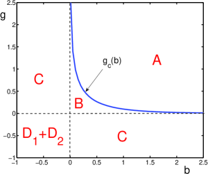
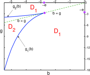
Figure 1: Regions on the plane $b-g$, as discussed in the text. In region $A$, there are no fixed points. In region $B$, there exist two fixed points, one being a stable node, while the other is a saddle. Region $C$ contains one fixed point being a stable focus. Region $D$ is subdivided into two subregions shown in more details in the right panel. In region $D_{1}$, there is one stable fixed point, being a stable node. In region $D_{2}$, there are three fixed points, two of them being stable nodes, while the third is a saddle.

4 Growth-Rate Acceleration of Population Dynamics

Since the stationary states, defined by equations (20), do not depend on the growth rate $\alpha$, it is reasonable to expect that the increase of the latter should result only in the acceleration of the temporal dynamics of the symbiotic populations, without qualitative changes in the overall picture. In many cases, it is really so, as is explained below.

4.1 Strong mutualistic growth of populations

In region $A$, where there are no fixed points, mutualistic populations grow faster when increasing the growth rate $\alpha$, displaying the same qualitative behavior, as is illustrated in Fig. 2.

                      

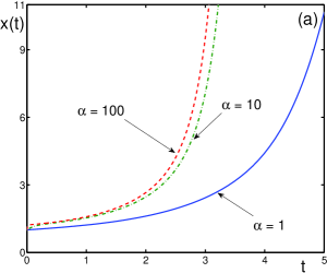
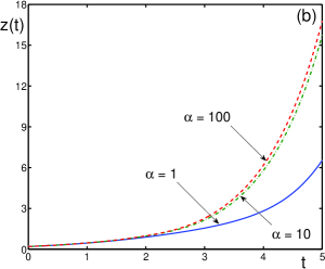
Figure 2: Dynamics of populations $x(t)$ and $z(t)$ in the parametric region $A$, for different growth rates. Here $b=1$ and $g=0.5>g_{c}\approx 0.0973$. The initial conditions are $\{x_{0}=1,z_{0}=0.2\}$. (a) Population $x(t)$ for $\alpha=1$ (solid line), $\alpha=10$ (dashed-dotted line), and $\alpha=100$ (dashed line); (b) population $z(t)$ for $\alpha=1$ (solid line), $\alpha=10$ (dashed-dotted line), and $\alpha=100$ (dashed line).

4.2 Convergence to single stationary states

In region $C$, there is just a single fixed point, being a stable focus. The convergence to the stationary state can be of slightly different type, as is shown in Figs. 3 and 4, but it is always faster when the parameter $\alpha$ is larger. The phase portrait is presented in Fig. 5.

The region $D_{1}$ contains a single stationary state, a stable node. Again, the convergence to the stationary state is faster when the growth rate $\alpha$ is larger, as is shown in Fig. 6.

                      

                      

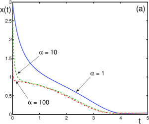
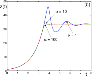
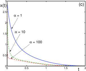
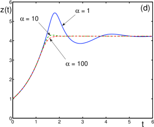
Figure 3: Dynamics of populations $x(t)$ and $z(t)$ in the parametric region $C$, for different $b<0$ and $g=100>0$. The initial conditions are $x_{0}=3$ and $z_{0}=1$. (a) Population $x(t)$, with $b=-0.1$, for $\alpha=1$ (solid line), $\alpha=10$ (dashed line), and $\alpha=100$ (dashed-dotted line). The stable fixed point is $x^{*}=0.035113$. (b) Population $z(t)$, with $b=-0.1$, for $\alpha=1$ (solid line), $\alpha=10$ (dashed line), and $\alpha=100$ (dashed-dotted line). The stable fixed point is $z^{*}=33.4918$. (c) Population $x(t)$, with $b=-1$, for $\alpha=1$ (solid line), $\alpha=10$ (dashed line), and $\alpha=100$ (dashed-dotted line). The stable fixed point is $x^{*}=0.01444$. (d) Population $z(t)$, with $b=-1$, for $\alpha=1$ (solid line), $\alpha=10$ (dashed line), and $\alpha=100$ (dashed-dotted line). The stable fixed point is $z^{*}=4.23773$.

                      

                      

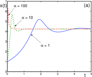
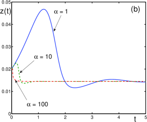
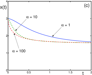
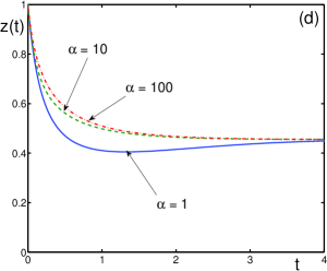
Figure 4: Dynamics of populations $x(t)$ and $z(t)$ in the parametric region $C$ for different initial conditions and different growth rates, when $b>0$, while $g<0$. (a) Population $x(t)$, with the symbiotic parameters $b=100$ and $g=-1$. The initial conditions are $x_{0}=1$ and $z_{0}=0.02$. The growth rate is $\alpha=1$ (solid line), $\alpha=10$ (dashed line), and $\alpha=100$ (dashed-dotted line). The stable fixed point is $x^{*}=4.2377$. (b) Population $z(t)$ for the same symbiotic parameters and initial conditions as in (a) for the growth rates $\alpha=1$ (solid line), $\alpha=10$ (dashed line), and $\alpha=100$ (dashed-dotted line). The stationary state is $z^{*}=0.01444$. (c) Population $x(t)$, with the symbiotic parameters $b=1$ and $g=-0.5$. The initial conditions are $x_{0}=3$ and $z_{0}=1$. Growth rate is $\alpha=1$ (solid line), $\alpha=10$ (dashed line), and $\alpha=100$ (dashed-dotted line). The stationary state is $x^{*}=1.5758$. (d) Population $z(t)$ for the same symbiotic parameters and initial conditions, as in (c), for $\alpha=1$ (solid line), $\alpha=10$ (dashed line), and $\alpha=100$ (dashed-dotted line). The stationary state is $z^{*}=0.45479$.

                      

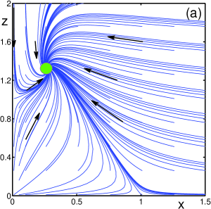
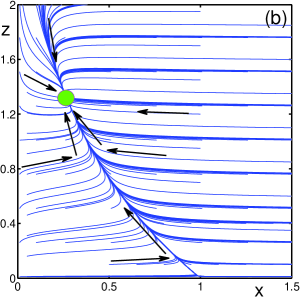
Figure 5: Phase portrait on the plane $x-z$, for the parametric region $C$, for $b=-1$ and $g=1$, and different growth rates $\alpha$. There exists a single fixed point, a stable focus, shown by the filled green disc. The fixed point is $\{x_{1}^{*}=0.26987,z_{1}^{*}=1.3098\}$. (a) Phase portrait for $\alpha=1$; (b) phase portrait for $\alpha=10$.

                      

                      

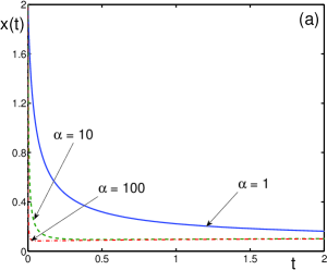
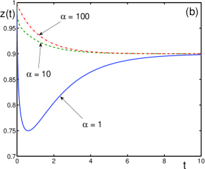
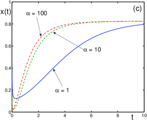
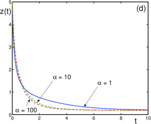
Figure 6: Dynamics of populations $x(t)$ and $z(t)$ in the region $D_{1}$, for different symbiotic parameters and initial conditions. (a) Population $x(t)$, with $b=-2.5$ and $g=-1$, and the initial conditions $\{x_{0}=2,z_{0}=1\}$, for $\alpha=1$ (solid line), $\alpha=10$ (dashed line), and $\alpha=100$ (dashed-dotted line). The stable fixed point is $x^{*}=0.10541$. (b) Population $z(t)$, for the same symbiotic parameters and initial conditions, as in (a), for $\alpha=1$ (solid line), $\alpha=10$ (dashed line), and $\alpha=100$ (dashed-dotted line). The fixed point is $z^{*}=0.89995$. (c) Population $x(t)$, with $b=-1$ and $g=-2$, initial conditions $\{x_{0}=0.4,z_{0}=5\}$, for $\alpha=1$ (solid line), $\alpha=10$ (dashed line), and $\alpha=100$ (dashed-dotted line). The fixed point is $x^{*}=0.82539$. (d) Population $z(t)$ for the same symbiotic parameters and initial conditions, as in (c), for $\alpha=1$ (solid line), $\alpha=10$ (dashed line), and $\alpha=100$ (dashed-dotted line). The fixed point is $z^{*}=0.19190$.

4.3 Convergent behavior in marginal cases

The marginal cases correspond to zero values of symbiotic parameters. Thus, if $b=0$, while $g$ is arbitrary, the sole stationary state is the stable node

$$x^{*}=1\;,\qquad z^{*}=e^{g}\qquad(b=0,~{}-\infty<g<\infty)\;,$$

with the characteristic exponents $\lambda_{1}=-1$ and $\lambda_{2}=-\alpha$. The population $x$ is described by the explicit formula

$$x=\frac{x_{0}}{x_{0}+(1-x_{0})\exp(-\alpha t)}\;.$$

The convergence to the stationary state is faster for larger $\alpha$.

When $b$ is arbitrary, while $g=0$, then again there exits just a single fixed point, a stable node

$$x^{*}=e^{b}\;,\qquad z^{*}=1\;,$$

with the characteristic exponents $\lambda_{1}=-\alpha$ and $\lambda_{2}=-1$. The population $z$ does not depend on $\alpha$, being given by the expression

$$z=\frac{z_{0}}{z_{0}+(1-z_{0})\exp(-t)}\;,$$

while the population $x$ converges to the stationary state faster for larger $\alpha$.

The examples of the present section illustrate the expected situation, where the growth rate $\alpha$ directly influences the time scales of the dynamics of the symbiotic populations, but does not qualitatively distort the overall picture.

5 Growth-Rate Induced Dynamic Transitions

In the present section, we show that there may happen unexpected situations, when the variation of the growth rate, although not influencing the stationary states, can lead to dramatic changes in the population dynamics.

5.1 Dynamic transition under mutualism

In the parametric region $B$, where $b>0$ and $0<g<g_{c}(b)$, there exist two fixed points, $\{x^{*}_{1},z^{*}_{1}\}$ and $\{x^{*}_{2},z^{*}_{2}\}$, with $1<x^{*}_{1}<x^{*}_{2}$ and $1<z^{*}_{1}<z^{*}_{2}$. The fixed point $\{x^{*}_{1},z^{*}_{1}\}$ is a stable node and $\{x^{*}_{2},z^{*}_{2}\}$ is a saddle. The stable node possesses a basin of attraction, whose boundary passes through the saddle. The behavior of the populations $x(t)$ and $z(t)$ depends on whether the initial conditions are taken inside the basin of attraction or not.

On the line $\{b,g_{c}(b)\}$, the stable node $\{x^{*}_{1},z^{*}_{1}\}$, and the saddle $\{x^{*}_{2},z^{*}_{2}\}$ merge together and disappear for $g>g_{c}(b)$. When $g=g_{c}(b)$, then $x_{1}^{*}=x_{2}^{*}$ and $z_{1}^{*}=z_{2}^{*}$.

It turns out that the growth rate $\alpha$, although not influencing the stationary states as such, does influence the boundary of the attraction basin. Therefore, it may happen that the same initial conditions, depending on the value of $\alpha$, can occur inside the attraction basin or outside it. This delicate situation is illustrated in Figs. 7 to 9.

Figure 7 demonstrates the convergence of the populations $x(t)$ and $z(t)$ for $g$ taken close to the line $\{b,g_{c}(b)\}$, with initial conditions that are inside the attraction basin of the stable fixed point for all $\alpha=1,10,100$. But in Fig. 8, the initial conditions $\{x_{0},z_{0}\}$ are such that they are outside of the basin of attraction for $\alpha=1$, but inside it, when $\alpha=10$ and $\alpha=100$. Contrary to Fig. 8, in Fig. 9, we show the situation when the initial conditions $\{x_{0},z_{0}\}$ are inside the basin of attraction of the stable fixed point for $\alpha=1$, but outside of it for $\alpha=10$ and $\alpha=100$. Phase portraits for region $B$, under different $\alpha$, are presented in Fig. 10. The boundary of the attraction basin essentially depends on the symbiotic parameters $b$ and $g$, as well as on the growth rate $\alpha$.

                      

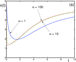
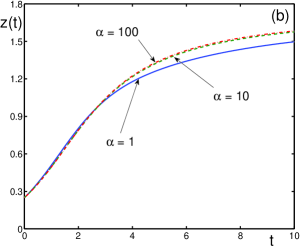
Figure 7: Dynamics of populations $x(t)$ and $z(t)$ in the parametric region $B$, with $b=1$ and $g=0.0972<g_{c}\approx 0.0973$, and the initial conditions $\{x_{0}=6,z_{0}=0.25\}$, such that the initial point is inside the attraction basin for all $\alpha=1,10,100$. The stable fixed point is $\{x^{*}_{1}=5.6717,z^{*}_{1}=1.7355\}$, and the saddle is $\{x^{*}_{2}=5.9995,z^{*}_{2}=1.7917\}$. (a) Population $x(t)$ for $\alpha=1$ (solid line), $\alpha=10$ (dashed line), and $\alpha=100$ (dashed-dotted line); (b) population $z(t)$ for $\alpha=1$ (solid line), $\alpha=10$ (dashed line), and $\alpha=100$ (dashed-dotted line).

                      

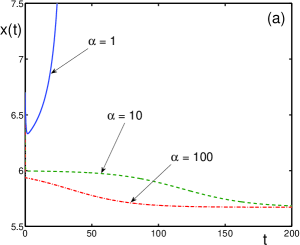
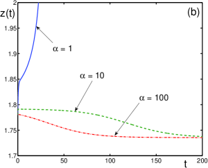
Figure 8: Dynamics of populations $x(t)$ and $z(t)$ for the parametric region $B$, with $b=1$ and $g=0.0972<g_{c}\approx 0.0973$, as in figure 7. The stable fixed point is $\{x^{*}_{1}=5.6717,z^{*}_{1}=1.7355\}$. The saddle is $\{x^{*}_{2}=5.9995,z^{*}_{2}=1.7917\}$, also as in figure 7. The initial conditions $\{x_{0}=6.7,z_{0}=1.78\}$ are such that they are outside of the attraction basin for $\alpha=1$, but inside for $\alpha=10$ and $\alpha=100$. (a) Population $x(t)$ for $\alpha=1$ (solid line), $\alpha=10$ (dashed line), and $\alpha=100$ (dashed-dotted line); (b) population $z(t)$ for $\alpha=1$ (solid line), $\alpha=10$ (dashed line), and $\alpha=100$ (dashed-dotted line).

                      

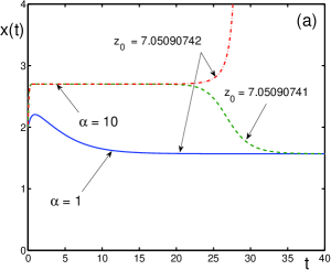
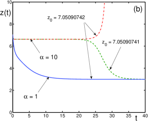
Figure 9: Dynamics of populations $x(t)$ and $z(t)$ in the parametric region $B$, with $b=0.15$ and $g=0.7<g_{c}\approx 0.76584$. The initial condition $x_{0}=2$ is fixed and $z_{0}$ is varied close to the boundaries of the attraction basins. The stable fixed point is $\{x^{*}_{1}=1.56721,z^{*}_{1}=2.9953\}$, and the saddle is $\{x^{*}_{2}=2.7011,z^{*}_{2}=6.6243\}$. (a) Population $x(t)$ for $\alpha=1$ and $z_{0}=7.05090742$ (solid line), for $\alpha=10$ and $z_{0}=7.05090742$ (dashed-dotted line), and for $\alpha=10$ but $z_{0}=7.05090741$ (dashed line); (b) population $z(t)$ for $\alpha=1$ and $z_{0}=7.05090742$ (solid line), for $\alpha=10$ and $z_{0}=7.05090742$ (dashed-dotted line), and for $\alpha=10$ but $z_{0}=7.05090741$ (dashed line).

                   

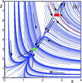
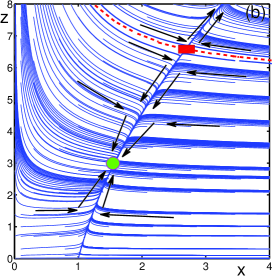
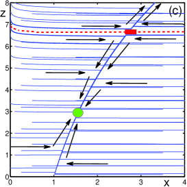
Figure 10: Phase portraits in the plane $x-z$ for the parametric region $B$, for the symbiotic parameters $b=0.15$ and $g=0.7$ and different growth rates $\alpha$. The stable node $\{x_{1}^{*}=1.56721,z_{1}^{*}=2.9953\}$ is denoted by the green filled disc, and the saddle $\{x_{2}^{*}=2.7011,z_{2}^{*}=6.6243\}$, by a red filled rectangle. The boundary of the basin of attraction is shown by the dashed line. (a) Phase portrait for $\alpha=1$; (b) phase portrait for $\alpha=10$; (c) phase portrait for $\alpha=500$.

5.2 Dynamic transition under parasitism

In the parametric region $D_{2}$, there exist three fixed points, such that $1>x_{1}^{*}>x_{2}^{*}>x_{3}^{*}$ and $z_{1}^{*}<z_{2}^{*}<z_{3}^{*}<1$. The points $\{x_{1}^{*},z_{1}^{*}\}$ and $\{x_{3}^{*},z_{3}^{*}\}$ are stable nodes, while $\{x_{2}^{*},z_{2}^{*}\}$ is a saddle. In the region $D_{2}$, the behavior of populations depends on initial conditions $\{x_{0},z_{0}\}$ and on the growth rate $\alpha$. With increasing time, the populations $x(t)$ and $z(t)$ can tend either to $\{x^{*}_{1},z^{*}_{1}\}$ or to $\{x^{*}_{3},z^{*}_{3}\}$, depending on the chosen initial conditions. The location of the boundary between the attraction basins, corresponding to different fixed points, strongly depends on the growth rate $\alpha$. The temporal behavior of the symbiotic populations is illustrated in Figs. 11, 12 and 13. Figures 14 and 15 present the related phase portraits for different growth rates.

                      

                      

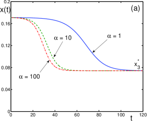
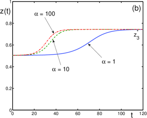
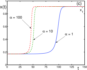
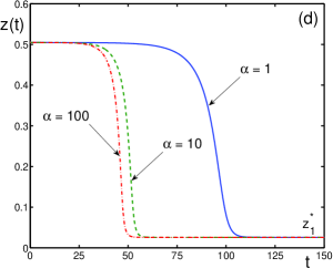
Figure 11: Dynamics of populations $x(t)$ and $z(t)$, in the parametric region $D_{2}$, for the symbiotic parameters $b=-3.5$ and $g=-4$, with the initial condition $x_{0}=0.171$ and different $z_{0}$ and $\alpha$. There are two stable nodes, $\{x_{1}^{*}=0.91332,z_{1}^{*}=0.02591\}$ and $\{x_{3}^{*}=0.074141,z_{3}^{*}=0.74337\}$, and the saddle $\{x_{2}^{*}=0.17099,z_{2}^{*}=0.50461\}$. (a) Population $x(t)$, with $z_{0}=0.505>z_{2}^{*}$, for $\alpha=1$ (solid line), $\alpha=10$ (dashed line), and $\alpha=100$ (dashed-dotted line); (b) population $z(t)$, with the same $z_{0}$, as in (a), for $\alpha=1$ (solid line), $\alpha=10$ (dashed line), and $\alpha=100$ (dashed-dotted line); (c) population $x(t)$, with $z_{0}=0.5046<z_{2}^{*}$, for $\alpha=1$ (solid line), $\alpha=10$ (dashed line), and $\alpha=100$ (dashed-dotted line); (d) population $z(t)$, with the same $z_{0}$, as in (c), for $\alpha=1$ (solid line), $\alpha=10$ (dashed line), and $\alpha=100$ (dashed-dotted line).

                      

                      

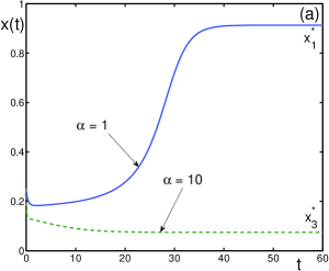
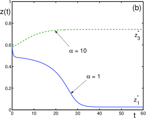
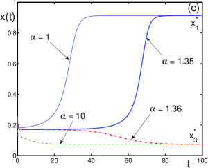
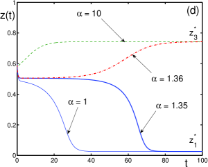
Figure 12: Dynamics of populations $x(t)$ and $z(t)$, in the parametric region $D_{2}$, with $b=-3.5$ and $g=-4$ as in figure 11, the initial conditions $x_{0}=0.25$ and $z_{0}=0.6$ for different growth rates $\alpha$. The stable nodes are $\{x_{1}^{*}=0.91332,z_{1}^{*}=0.02591\}$ and $\{x_{3}^{*}=0.074141,z_{3}^{*}=0.74337\}$ and the saddle is $\{x_{2}^{*}=0.17099,z_{2}^{*}=0.50461\}$, as in figure 11. (a) Population $x(t)$ for $\alpha=1$ (solid line) and $\alpha=10$ (dashed line); (b) population $z(t)$ for $\alpha=1$ (solid line) and $\alpha=10$ (dashed line); (c) population $x(t)$ for $\alpha=1$ (thin solid line), $\alpha=1.35$ (solid line), $\alpha=1.36$ (dashed-dotted line), and $\alpha=10$ (thin dashed line); (d) population $z(t)$ for $\alpha=1$ (thin solid line), $\alpha=1.35$ (solid line), $\alpha=1.36$ (dashed-dotted line), and $\alpha=10$ (thin dashed line). For the given parameters, there exists the critical value $\alpha_{crit}$ of the growth rate, such that $1.35<\alpha_{crit}<1.36$. Under the same initial conditions, if $1\leq\alpha<\alpha_{crit}$, then the populations tend to the node $\{x_{1}^{*}=0.91332,z_{1}^{*}=0.02591\}$, while when $\alpha>\alpha_{crit}$, the populations converge to the other node $\{x_{3}^{*}=0.074141,z_{3}^{*}=0.74337\}$.

                      

                      

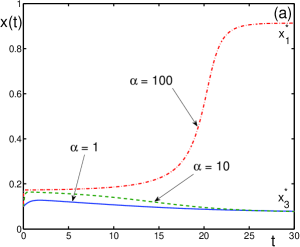
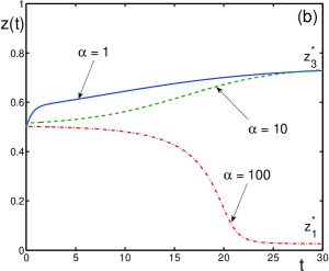
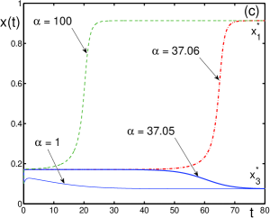
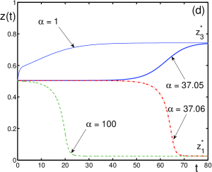
Figure 13: Dynamics of populations $x(t)$ and $z(t)$, in the parametric region $D_{2}$, with $b=-3.5$ and $g=-4$, the initial conditions $x_{0}=0.1$ and $z_{0}=0.5$, for different $\alpha$. The stable nodes are $\{x_{1}^{*}=0.91332,z_{1}^{*}=0.02591\}$ and $\{x_{3}^{*}=0.074141,z_{3}^{*}=0.74337\}$ and the saddle is $\{x_{2}^{*}=0.17099,z_{2}^{*}=0.50461\}$, as in figs. 11 and 12. (a) Population $x(t)$ for $\alpha=1$ (solid line), $\alpha=10$ (dashed line), and $\alpha=100$ (dashed-dotted line); (b) population $z(t)$ for $\alpha=1$ (solid line), $\alpha=10$ (dashed line), and $\alpha=100$ (dashed-dotted line); (c) population $x(t)$ for $\alpha=1$ (thin solid line), $\alpha=37.05$ (solid line), $\alpha=37.06$ (dashed-dotted line), and $\alpha=100$ (thin dashed line); (d) population $z(t)$ for $\alpha=1$ (thin solid line), $\alpha=37.05$ (solid line), $\alpha=37.06$ (dashed-dotted line), and $\alpha=100$ (thin dashed line). There exists the critical growth rate $\alpha_{crit}$ in the interval $37.05<\alpha_{crit}<37.06$, such that, when $1\leq\alpha<\alpha_{crit}$, the populations tend to the node $\{x_{3}^{*}=0.074141,z_{3}^{*}=0.74337\}$, while if $\alpha>\alpha_{crit}$, the populations converge to the node $\{x_{1}^{*}=0.91332,z_{1}^{*}=0.02591\}$.

                   

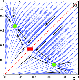
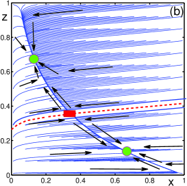
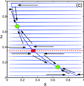
Figure 14: Phase portraits on the plane $x-z$ for the parametric region $D_{2}$, with $b=g=-3$, for different $\alpha$. The dashed line shows the boundary between the attraction basins of the stable nodes $\{x_{1}^{*}=0.66474,z_{1}^{*}=0.13612\}$ and $\{x_{3}^{*}=0.13612,z_{3}^{*}=0.66474\}$, which are represented by the filled green discs. The saddle point $\{x_{2}^{*}=z_{2}^{*}=0.34997\}$ is shown by the filled red rectangle. (a) Phase portrait for $\alpha=1$, which exhibits a symmetric boundary line given by the equation $x=z$ (dashed line); (b) phase portrait for $\alpha=10$; (c) phase portrait for $\alpha=200$. For large growth rates $\alpha\rightarrow\infty$, the boundary between the attraction basins tends to the line $z=z_{2}^{*}$.

                   

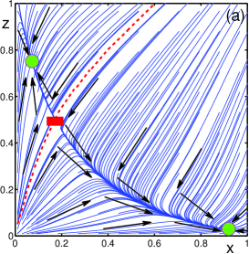
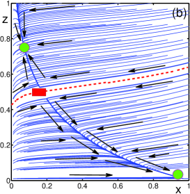
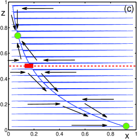
Figure 15: Phase portraits on the plane $x-z$ for the parametric region $D_{2}$, with $b=-3.5$ and $g=-4$, for different $\alpha$. The dashed line shows the boundary between the attraction basins of the stable nodes $\{x_{1}^{*}=0.91332,z_{1}^{*}=0.02591\}$ and $\{x_{3}^{*}=0.074141,z_{3}^{*}=0.74337\}$, which are represented by the filled green discs. The saddle point $\{x_{2}^{*}=0.17099,z_{2}^{*}=0.50461\}$ is indicated by the filled red rectangle. (a) Phase portrait for $\alpha=1$; (b) phase portrait for $\alpha=10$; (c) phase portrait for $\alpha=200$. In the limit of large $\alpha$’s, the boundary between the attraction basins tends to the line $z=z_{2}^{*}$.

6 Approximate Solutions of Symbiotic Equations in the Presence of Coexisting Fast and Slow Populations

For large growth rates $\alpha\gg 1$, equations (18) imply that the variable $x$ is fast while the variable $z$ is slow. In this case, the analysis of the evolution equations can be done by resorting to the Bogolubov-Krylov averaging techniques Bogolubov & Mitropolsky [1961]. As is described in the scale-separation approach Yukalov [1993], we solve the equation for the fast variable, keeping the slow variable as a quasi-integral of motion, which gives

$$x=\frac{x_{0}}{x_{0}(1-e^{-\alpha t})e^{-bz}+e^{-\alpha t}}\;.$$ (33)

This expression is substituted into the equation for the slow variable, which is averaged over time, resulting in the equation

$$\frac{dz}{dt}=z-z^{2}\exp\left(-ge^{bz}\right)\;.$$ (34)

Equations (33) and (33) define the so-called guiding centers of the solutions to equations (18).

In Figures 16 and 17, we demonstrate that the guiding-center solutions, prescribed by equations (33) and (34), provide rather good approximations for the exact solutions following from the initial equations (18). Surprisingly, the approximate solutions are already rather close to the true solutions even for $\alpha=1$. The stationary states are identical for the approximate solutions and for exact ones.

                      

                      

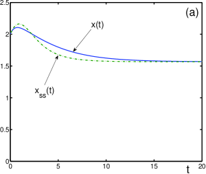
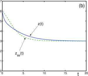
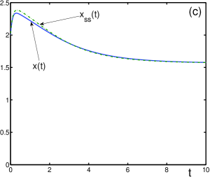
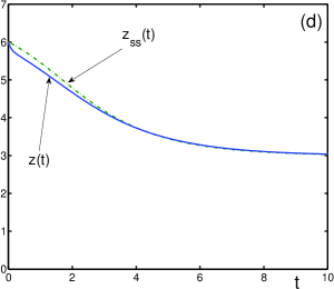
Figure 16: Temporal behavior of approximate solutions $x_{ss}(t)$ and $z_{ss}(t)$, obtained by the scale separation approach, as compared to the exact solutions $x(t)$ and $z(t)$, for the case of mutualism, with the symbiotic parameters $b=0.15$ and $g=0.7$, with the initial conditions $\{x_{0}=2,z_{0}=6\}$, for different growth rates $\alpha$. The stable stationary state is $\{x^{*}=1.56721,z^{*}=2.9953\}$. (a) Population $x(t)$ (solid line) and its approximation $x_{ss}(t)$ (dashed-dotted line) for $\alpha=1$; (b) population $z(t)$ (solid line) and its approximation $z_{ss}(t)$ (dashed-dotted line) for $\alpha=1$; (c) population $x(t)$ (solid line) and its approximation $x_{ss}(t)$ (dashed-dotted line) for $\alpha=10$; (d) population $z(t)$ (solid line) and its approximation $z_{ss}(t)$ (dashed-dotted line) for $\alpha=10$.

                      

                      

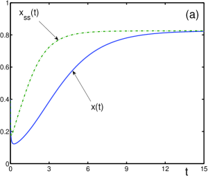
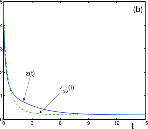
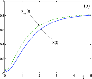
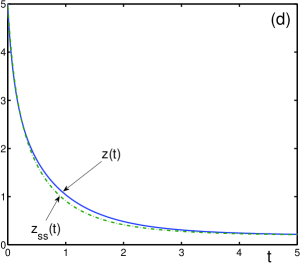
Figure 17: Temporal behavior of approximate solutions $x_{ss}(t)$ and $z_{ss}(t)$, obtained by the scale separation approach, as compared to the exact solutions $x(t)$ and $z(t)$, for the case of parasitism, with the symbiotic parameters $b=-1$ and $g=-2$, with the initial conditions $x_{0}=0.4$ and $z_{0}=5$, for different growth rates $\alpha$. The stable stationary state is $\{x^{*}=0.82539,z^{*}=0.1919\}$. (a) Population $x(t)$ (solid line) and its approximation $x_{ss}(t)$ (dashed-dotted line) for $\alpha=1$; (b) population $z(t)$ (solid line) and its approximation $z_{ss}(t)$ (dashed-dotted line) for $\alpha=1$; (c) population $x(t)$ (solid line) and its approximation $x_{ss}(t)$ (dashed-dotted line) for $\alpha=10$; (d) population $z(t)$ (solid line) and its approximation $z_{ss}(t)$ (dashed-dotted line) for $\alpha=10$.

7 Conclusion

In the case of a standard dynamic transition, a qualitative change of dynamical behavior occurs when a system parameter reaches a bifurcation point, where the nature of fixed points changes. We have demonstrated the existence of a non-standard dynamic transition, in which a qualitative change of dynamical behavior occurs as a result of the variation of the growth rate that does not influence the fixed points. The sharp change in dynamical behavior happens because the varying growth rate shifts the boundary of the basins of attraction of the fixed points, while the fixed points themselves do not change. Typically, the initial point of a trajectory, which was inside the attraction basin of the stable point for a first value of the growth rate, can happen to be found outside of it due to the change of the shape of the attraction basin for a different value of the growth rate, or vice versa.

We have illustrated this dynamic transition, caused by the distortion of the shape of the basin of attraction, using a dynamical system describing the evolution of symbiotic species with different growth rates. The effect can happen under mutualism as well as under parasitism of the co-evolving species. As has been explained earlier Yukalov et al. [2012a, b, 2014a, 2015], the considered symbiotic equations can characterize various biological and social systems. Biological systems have also much in common with economical systems Trenchard & Perc [2016] as well as with structured human societies Perc [2016]. Therefore the described effect can occur in different nonlinear dynamical systems.

As an example, where the described effect does happen in nature, it is possible to mention the ubiquitous symbiosis between fungi and plants. The proliferation of the Arbuscular Mycorrhizal fungi network at a late stage in plant life is well established to be beneficial for plant growth and reproduction Kapulnik & Douds [2000]; Smith & Read [2008]. However, a too fast proliferation of this fungi at the early stage of the plant life cycle can lead to the suppression of plant seedling due to the carbon cost associated with sustaining the fungi Varga & Kytöviita [2016]; Koide [1985]; Johnson et al. [1997]; Ronsheim [2012]. Here, the early or late plant life stage correspond to different initial conditions, when the plant is either still small or already mature. Depending on these initial conditions, the same fungi growth rate can be either beneficial for the plant or suppressing it, similarly to the cases considered in our article.

Acknowledgments We acknowledge financial support from the ETH Zürich Risk Center.

References

Ahmadjian & Paracer [2000]
Ahmadjian, V. & Paracer, S. [2000]
Symbiosis: An Introduction to Biological Associations
(Oxford University, Oxford).
Bennett & Moran [2015]
Bennett, G.M. & Moran, N.A. [2015]
“Heritable symbiosis: the advantage and perils of an evolutionary rabbit hole,”
Proc. Nat. Acad. Sci.112, 10169–10176.
Bogolubov & Mitropolsky [1961]
Bogolubov, N.N. & Mitropolsky, Y.A. [1961]
Asymptotic Methods in the Theory of Nonlinear Oscillations
(Gordon and Breach, New York).
Boucher [1988]
Boucher, D. [1988]
The Biology of Mutualism: Ecology and Evolution
(Oxford University, New York).
Cunning & Baker [2014]
Cunning, R. & Baker, A.C. [2014]
“Not just two, but how many: the importance of partner abundance in reef
coral symbioses,”
Front. Microbiol.5, 400.
Di Prisco et al. [2016]
Di Prisco, G., Annoscia, D., Margiotta, M., Ferrara, R., Varricchio, P.,
Zanna, V., Caprio, E., Nazzi, F. & Pennacchio, F. [2016]
“A mutualistic symbiosis between a parasitic mite and a pathogenic virus
undermines honey bee immunity and health,”
Proc. Nat. Acad. Sci.113, 3203 3208.
Douglas [1984]
Douglas, A.E. [1984]
Symbiotic Interactions
(Oxford University, Oxford).
Johnson et al. [1997]
Johnson, N.C., Graham, J.H. & Smith, F.A. [1997]
“Functioning of mycorrhizal associations along the mutualism-parasitism continuum,”
New Phytologist135, 575–585.
Kapulnik & Douds [2000]
Kapulnik, Y. & Douds, D.D. eds. [2000]
Arbuscular Mycorrhizas Physisology and Function
(Kluwer Academic, Dordrecht).
Koide [1985]
Koide, R. [1985]
“The nature of growth depression in sunflower caused by vesicular-arbuscular
mycorrhizal infection,”
New Phytologist99, 449–462.
Ley et al. [2006]
Ley, R., Peterson, D. & Gordon, J. [2006]
“Ecological and evolutionary forces shaping microbial diversity in the human intestine,”
Cell124, 837–848.
Ley et al. [2008]
Ley, R.E., Hamady, M., Lozupone, C., Turnbaugh, P., Ramey, R.R., Bircher, J.S.,
Schlegel, M.L., Tucker, T.A., Schrenzel, M.D., Knight, R. & Gordon, J.I. [2008]
“Evolution of mammals and their gut microbes,”
Science320, 1647–1651.
Perc [2016]
Perc, M., [2016]
“Phase transitions in models of human cooperation,”
Phys. Lett. A380, 2803–2808.
Rodriguez et al. [2009]
Rodriguez, R.J., Freeman, D.C., McArthur, E.D., Kim, Y.O. & Redman, R.S. [2009]
“Symbiotic regulations of plant growth, development and reproduction,”
Commun. Integr. Biol. 2, 141–143.
Ronsheim [2012]
Ronsheim, M.L. [2012]
“The effect of mycorrhizae on plant growth and reproduction varies with
soil phosphorous and developmental stage,”
Am. Midland Naturalist167, 28–39.
Sapp [1994]
Sapp, J. [1994]
Evolution by Association: A History of Symbiosis
(Oxford University, Oxford).
Trenchard & Perc [2016]
Trenchard, H. & Perc, M. [2016]
“Equivalences in biological and economical systems: Peloton dynamics and the rebound
effect,”
PLOS One11, e0155395.
Varga & Kytöviita [2016]
Varga, S. & Kytöviita, M.M. [2016]
“Faster acquisition of symbiotic partner by common mycorrhizal networks
in early life stage,”
Ecosphere7, 01222.
Yukalov [1991]
Yukalov, V.I. [1991]
“Method of self-similar approximations,”
J. Math. Phys.32, 1235–1239.
Yukalov [1992]
Yukalov, V.I. [1992]
“Stability conditions for method of self-similar approximations,”
J. Math. Phys.33, 3994–4001.
Yukalov et al. [2009]
Yukalov, V.I., Yukalova, E.P. & Sornette, D. [2009]
“Punctuated evolution due to delayed carrying capacity,”
Physica D238, 1752–1767.
Yukalov et al. [2012a]
Yukalov, V.I., Yukalova, E.P. & Sornette, D. [2012a]
“Modeling symbiosis by interactions through species carrying capacities,”
Physica D241, 1270–1289.
Yukalov et al. [2012b]
Yukalov, V.I., Yukalova, E.P. & Sornette, D. [2012b]
“Extreme events in population dynamics with functional carrying capacity,”
Eur. Phys. J. Spec. Top.205, 313–354.
Yukalov et al. [2014a]
Yukalov, V.I., Yukalova, E.P. & Sornette, D. [2014a]
“Population dynamics with nonlinear delayed carrying capacity,”
Int. J. Bifur. Chaos24, 1450021.
Yukalov et al. [2014b]
Yukalov, V.I., Yukalova, E.P. & Sornette, D. [2014b]
“New approach to modeling symbiosis in biological and social systems,”
Int. J. Bifur. Chaos24, 1450117.
Yukalov et al. [2015]
Yukalov, V.I., Yukalova, E.P. & Sornette, D. [2015]
“Dynamical system theory of periodically collapsing bubbles,”
Eur. Phys. J. B88, 179.