Modulation of localized solutions in quadratic-cubic nonlinear Schrödinger equation with inhomogeneous coefficients

Abstract

We study the presence of exact localized solutions in a quadratic-cubic nonlinear Schrödinger equation with inhomogeneous nonlinearities. Using a specific ansatz, we transform the nonautonomous nonlinear equation into an autonomous one, which engenders composed states corresponding to solutions localized in space, with an oscillating behavior in time. Direct numerical simulations are employed to verify the stability of the modulated solutions against small random perturbations.

1 Introduction

Localized solutions in nonlinear media such as the shape preserving solitons, and breathers, which are characterized by internal oscillations, have fundamental applications for energy transport in optical fibers and waveguides [1, 2], polaronic materials [3], biological molecules [4], etc. These solutions can propagate without losing their shape due to equilibrium between diffraction (in spatial domain) or dispersion (in temporal domain) and nonlinearity [5, 6, 7, 8]. They also appear describing localized excitations in dilute Bose-Einstein condensates in specific conditions of balance between the particle dispersion and the nonlinear effect due to the two-body interaction [9, 10] and open possibilities for future applications in coherent atom optics, atom interferometry, and atom transport.

In many cases, the equations that describe the systems have the form of a nonlinear Schrödinger (NLS) equation [11]. Indeed, the NLS equation appears as a universal equation governing the evolution of slowly varying packets of quasi-monochromatic waves in weakly nonlinear media featuring dispersion. One can exemplify this with: light propagation in nonlinear optical fibers and planar waveguides; small-amplitude gravity waves on the surface of deep inviscid water and Langmuir waves in hot plasmas; interaction of high-frequency molecular vibrations and low-frequency longitudinal deformations in a model of long biological molecules; mean-field description of Bose-Einstein condensates (in this case it becomes the Gross-Pitaevskii equation); models that describe nonlinear dissipative media (in this case it becomes the Ginzburg-Landau equation); and so on. Regarding the form of the nonlinearities in the NLS equation one can find: quadratic [12], quadratic-cubic [13, 14], cubic (or Kerr-type) [1, 15, 16], cubic-quintic [17, 18, 19, 20], quintic [21, 22], nonpolynomial [23, 24, 25, 26, 27, 28], logarithm [29, 30], saturable [31, 32, 33], and other nonlinearities.

The inclusion of variable coefficients in the NLS equation, which are due to inhomogeneities, produces a gigantic backdrop of possibilities of modulation of the localized solutions, although it breaks the integrability of the standard cubic NLS equation [34]. Physically, the variable coefficients can be achieved by changing the system structure, as for example, in the magnetohydrodynamics the inhomogeneity of the real plasma environment can be achieved by fluctuations of the density, temperature, and magnetic fields [35]; the inhomogeneities in nonlinear fibers or crystals are due to variation in the geometry and/or variation in the material parameters in the fabrication process of such systems [1]; in Bose-Einstein condensates (BECs) the variations in the potential and nonlinearities can be controlled by the application of external fields, which also induce modulation pattern of the local nonlinearity through the Feshbach-resonance mechanism, i.e., field-induced changes of the scattering length characterizing binary collisions between atoms, which contributes to modify the nonlinearity in the BEC [36].

The construction of analytical solitonic solutions is a hard task. However, by applying a similarity transformation technique, which transforms the nonautonomous NLS equation into an autonomous one, one can build analytical solutions. This method has been applied in a number of works [37, 38, 39, 40, 41, 42, 43, 44, 45, 46, 47, 48, 49, 50, 51, 52, 27, 53, 54, 55, 56, 30, 57, 58, 59, 60, 61]. In particular, in Ref. [37] the authors presented localized nonlinear waves in systems with time- and space-modulated cubic nonlinearities. More general models, including cubic-quintic nonlinearities and modulations with dependence on both time and space coordinates were considered in Refs. [19, 46, 48, 52, 49, 61]. Exact solutions to three-dimensional generalized NLS equations with varying potential and nonlinearities were studied in Refs. [38, 39, 40]. Also, the modulation of breathers and rogue waves were investigated in Refs. [40, 42] and Refs. [47, 50, 58], respectively. In Refs. [43, 51, 59], one investigated solitons of two-component systems modulated in space and time. Moreover, in Ref. [53] one studied solitons in a generalized model, using space- and time-variable coefficients in a NLS equation with higher-order terms. More recently, the dynamics of self-similar waves in asymmetric twin-core fibers with Airy-Bessel modulated nonlinearity was also investigated in [57].

These previous studies have motivated the investigations of other new possibilities, among them the quadratic-cubic nonlinear Schrödinger (QCNLS) equations with inhomogeneous coefficients, in the presence of several distinct background potentials. From the general physical perspective, QCNLS equations have received considerable attention in classical field theory [62] because the localized solutions are non-topological or lump-like structures [63] that appear in several contexts in physics such as q-balls, tachyon branes, and galactic dark matter properties (see [64] and references therein). In BEC, these equations can arise as an approximate model of a relatively dense quasi-1D BEC with repulsive local interactions between atoms [25, 65] plus a long-range dipole-dipole attraction between them [66]. Recently, the presence of chaotic solitons in this system under nonlinearity management has been investigated in [14] via numerical simulations and variational approximation with rational and hyperbolic trial functions. In the current work, our goal is to find analytical solutions describing localized structures modulated by nonautonomous QCNLS equations, allowing us to investigate different patterns of modulations. To do this, we employ the similarity transformation technique and direct numerical simulations to check stability of the solutions. The problem is of current interest since we know that information on the stability of solitonic solutions is of great significance in the study of atomic Bose-Einstein condensates [10, 67].

The work is organized as follows. In Sec. 2 we introduce the theoretical model and apply the similarity transformation to get information on the pattern of the inhomogeneous terms of the QCNLS equation. Also, we present two different solutions of the autonomous QCNLS equation. The linear stability analysis is displayed in Sec. 3. Next, in the Sec. 4 we consider three different modulation patterns and show the results of the stability tests that are obtained via direct numerical simulations. We summarize our results and suggest new investigations in Sec. 5.

2 The quadratic-cubic model and the analytical solutions

The model of interest in this work is described by the QCNLS equation with inhomogeneous coefficients. It is given by

$$i\psi_{t}=-\frac{1}{2}\psi_{xx}+V(x,t)\psi+g_{2}(t)|\psi|\psi+g_{3}(t)|\psi|^{2}\psi,$$ (1)

where $\psi=\psi(x,t)$, $\psi_{t}=\partial\psi/\partial t$, $\psi_{xx}=\partial^{2}\psi/\partial x^{2}$, $V(x,t)$ is the background or trapping potential, and $g_{2}(t)$ and $g_{3}(t)$ represent the quadratic and cubic nonlinearity intensities, which are modulated in time, respectively. This second order partial differential equation with quadratic and cubic time-dependent nonlinearities is very hard to solve, but it describes very interesting physical systems such as cigar-shaped condensates with repulsive interatomic interactions [25] plus a dipole-dipole attraction [66], i.e, Eq. (1) appears as an effective 1D equation that governs the axial dynamics of mean-field cigar-shaped condensates and accounts accurately the contribution from the transverse degrees of freedom. Hence, our goal is to construct explicit nontrivial solutions of this QCNLS with potentials depending on the spatial coordinate and on time, with nonlinearities depending on time. To achieve this, we use the following ansatz [42]

$$\psi=\rho(t)e^{i\eta(x,t)}\Phi[\zeta(x,t),\tau(t)]$$ (2)

that connects the nonautonomous QCNLS to an autonomous QCNLS equation

$$i\Phi_{\tau}=-\frac{1}{2}\Phi_{\zeta\zeta}+G_{2}|\Phi|\Phi+G_{3}|\Phi|^{2}\Phi,$$ (3)

with constant coefficients $G_{2}$ and $G_{3}$, which is easier to solve. Note that the ansatz (2) transfer all the space and time dependence of the coefficients of (1) to the external parameters, the amplitude $\rho(t)$ and the phase $\eta(x,t)$, and now the new coordinates $\zeta(x,t)$ and $\tau(t)$ describe the space and time evolution in relation to a frame which is moving with the localized solution.

By inserting (2) into (1) one gets the Eq. (3) provided that the set of conditions

$$\rho_{t}+\frac{1}{2}\rho\eta_{xx} = 0,$$ (4)

$$\zeta_{t}+\zeta_{x}\eta_{x} = 0,$$ (5)

$$\tau_{t}-\zeta_{x}^{2} = 0,$$ (6)

$$\zeta_{xx} = 0.$$ (7)

are satisfied in order to connect the external parameters with the internal ones. These conditions are tightly related to each other, but they allow that we go on: for instance, from Eq. (7) one derives $\zeta(x,t)=a(t)x+b(t)$, where $a(t)$ is the inverse of the width of the localized solution (it is positive definite) and $-b(t)/a(t)$ is the position of its center of mass, which implies in Eq. (6) the following condition $\tau(t)=\int a^{2}dt$. Then, one can obtain the amplitude and phase of the ansatz (2), given by

$$\rho(t) = \sqrt{a},$$ (8)

$$\eta(x,t) = -\frac{a_{t}x^{2}}{2a}-\frac{b_{t}x}{a}+\epsilon(t),$$ (9)

respectively.

In addition, the trapping potential and nonlinear terms must have the form

$$V = -\eta_{t}-\frac{1}{2}\eta_{x}^{2},$$ (10)

$$g_{2} = G_{2}\frac{\zeta_{x}^{2}}{\rho},$$ (11)

$$g_{3} = G_{3}\frac{\zeta_{x}^{2}}{\rho^{2}}=\frac{G_{3}g_{2}}{G_{2}\rho},$$ (12)

which, by using the Eqs. (8) and (9), can be rewritten as

$$V(x,t) = \alpha(t)x^{2}+\beta(t)x+\delta(t),$$ (13)

$$g_{2}(t) = G_{2}a(t)^{3/2},$$ (14)

$$g_{3}(t) = G_{3}a(t),$$ (15)

where

$$\alpha(t) = \left(aa_{tt}-2a_{t}^{2}\right)/2a^{2},$$ (16)

$$\beta(t) = \left(ab_{tt}-2a_{t}b_{t}\right)/a^{2},$$ (17)

$$\delta(t) = -\left(2a^{2}\epsilon_{t}+b_{t}^{2}\right)/2a^{2}.$$ (18)

Note that the modulation in the present model is completely defined by setting the functions $a(t)$, $b(t)$, and $\epsilon(t)$. Physically, this can be done by setting appropriately the patterns of linear and nonlinear coefficients ($V$, $g_{2}$, and $g_{3}$, respectively) in the system. For example, in a BEC the harmonic potential and nonlinearities may vary in time due to the application of a modulated laser beam that controls the interactions optically.

Next, we go further on the subject and consider an interesting possibility, with the solution $\Phi=\varphi(\zeta)e^{-i\mu\tau}$ of Eq. (3), such that

$$\mu\varphi=-\frac{1}{2}\varphi_{\zeta\zeta}+G_{2}\varphi^{2}+G_{3}\varphi^{3},$$ (19)

where $\mu$ is a constant and $\varphi>0$. In this case, we can get two distinct solutions, the first one having the form

$$\varphi=\frac{A}{1+B\zeta^{2}},$$ (20)

with $A=-4G_{2}/3G_{3}$ (assuming $A>0$), $B=-4G_{2}^{2}/9G_{3}$ and $\mu=0$. Note that we need $B>0$ for a nonsingular solution, which implies that $G_{3}<0$ and $G_{2}>0$. The presence of a negative $G_{3}$ implies that the system engenders focusing cubic nonlinearity, and since $G_{2}$ is positive, one is dealing with a defocusing quadratic nonlinearity. Also, one can obtain a different solution

$$\varphi=\frac{A^{\prime}}{1+B^{\prime}\cosh(\zeta)}\,,$$ (21)

where $A^{\prime}=-3/(2G_{2})$, $B^{\prime}=-\sqrt{4G_{2}^{2}-9G_{3}}/(2G_{2})$ and $\mu=-1/2$. There are two ranges of values of $B^{\prime}$ that present nonsingular solutions, viz., $B^{\prime}>0$ implying $G_{2}<0$ and $G_{3}<4G_{2}^{2}/9$; $B^{\prime}<-1$ implying $G_{2}>0$ and $G_{3}<0$. Both cases are of current interest since they can present self-focusing or self-defocusing nonlinearities (competitive or not), which can correspond to different types of materials constituting the nonlinear fiber or the crystal [1].

3 Analysis of linear stability

To analyze the linear stability of our analytical solutions of the autonomous QCNLS equation, we perturbed it by normal modes as

$$\Phi(\zeta,\tau)=\left\{\varphi(\zeta)+[v(\zeta)+w(\zeta)]e^{\lambda\tau}+[v^{*}(\zeta)+w^{*}(\zeta)]e^{\lambda^{*}\tau}\right\}e^{-i\mu\tau},$$ (22)

where $v(\zeta),w(\zeta)\ll 1$ are normal-mode perturbations, and $\lambda$ is the eigenvalue of this normal mode. Inserting this perturbed solution in (3) and linearizing, we obtain the following linear-stability eigenvalue problem:

$$\mathbf{L}\Psi=\lambda\Psi,$$ (23)

where

$$\mathbf{L}=i\left(\begin{array}[]{cc}0&\frac{1}{2}\nabla^{2}+\mathcal{F}_{1}\\ \frac{1}{2}\nabla^{2}+\mathcal{F}_{2}&0\end{array}\right),\hskip 10.00002pt\Psi=\left(\begin{array}[]{c}v\\ w\end{array}\right),$$ (24)

and

$$\mathcal{F}_{1} = \mu-G_{2}\varphi-G_{3}\varphi^{2},$$

$$\mathcal{F}_{2} = \mu-2G_{2}\varphi-3G_{3}\varphi^{2},$$

where we have assumed $\varphi$ real and positive. Here we use the Fourier collocation method to compute eigenvalues of the linear-stability operator $\mathbf{L}$, in which one expands the eigenfunction $\Psi$ into a Fourier series and turns Eq. (23) into a matrix eigenvalue problem for the Fourier coefficients of the eigenfunction $\Psi$. One can find examples of application of this method in Ref. [34], and here we investigate the four new distinct possibilities which we describe below.

4 Analytical results and numerical simulations

We now examine the modulation of the above solutions and their stability by numerical simulations. The numerical method is based on the $4^{\mathrm{th}}$ order split-step Crank-Nicholson algorithm in which the evolution equation is split into several pieces (linear and nonlinear terms), which are integrated separately. To this end, we use the steps $\Delta x=0.04$ and $\Delta t=0.001$, providing a good accuracy during the evolution of the wave function, with fixed spatial width [-30,30]. Then, to study stability for the above cases we employ a random perturbation in the amplitude of the solution with the form

$$\psi=\psi_{0}[1+0.05v(x)],$$ (25)

where $\psi_{0}=\psi(x,0)$ is the analytical solution obtained via ansatz (2) and $v\in[-0.5,0.5]$ is a real random number with zero mean (white noise) evaluated at each point of discretization grid in $x$-coordinate. Also, to ensure the stability of the method we also checked the norm (power) and the energy of the solution defined by $P=\int_{-\infty}^{\infty}|\psi|^{2}dx$ and

$$E=\int_{-\infty}^{\infty}dx\left\{\frac{1}{2}|\psi_{x}|^{2}+V|\psi|^{2}+\frac{2}{3}g_{2}|\psi|^{3}+\frac{g_{3}}{2}|\psi|^{4}\right\},$$ (26)

respectively.

In order to focus on the practical use of the above results, in the following we present some specific examples of typical potentials and nonlinearities given by Eqs. (13)-(15) that can be found in experimental setups. Here, for pedagogical purpose, four distinct cases are addressed. In the first, presented in Subsec. 4.1, we consider the system without modulation, in order to give us a landmark about the stability of such solutions. In Subsec. 4.2 we include a potential which is asymmetric in space and periodically modulated in time, which is found by setting $\alpha(t)=\delta(t)=0$ and $\beta(t)\neq 0$. This type of potential is interesting because we can see how the center of mass of the solutions behave under a periodically oscillating uniform field. Another potential, the harmonically symmetric in space and periodically modulated in time potential, which is obtained with $\beta(t)=\delta(t)=0$ and $\alpha(t)\neq 0$, is studied in Subsec. 4.3. Here the main motivation is to investigate how the solutions behave under the effect of the squeezing and anti-squeezing produced by the oscilatting harmonic potential. Finally, a more general case, mixing the two previous cases, is considered in Subsec. 4.4.

Indeed, all patterns of potential and nonlinearities addressed here are feasible in several scenarios, for example, in nonlinear fiber optics and BECs [68, 69, 36]: the first case can be attained by the action of a periodic heterogeneity obtained in the fiber construction, and the second one may be driven by external potentials and by using the Feshbach-resonance management.

4.1 Vanishing potential

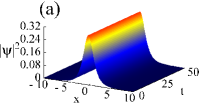
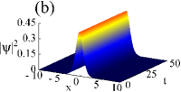
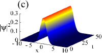
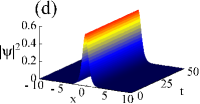
Figure 1: (Color online) Localized solutions $|\psi|^{2}$ obtained from the ansatz (2) without modulation ($\alpha=\beta=\delta=0$ by setting $a=1$, $b=0$, and $\epsilon=0$). We display the analytical results considering the static localized profiles given by Eq. (20) in (a) and Eq. (21) in (b)-(d). The values of the nonlinearities are (a) $G_{2}=5/4$ and $G_{3}=-3$ (case A), (b) $G_{2}=-2/3$ and $G_{3}=-1$ (case B), (c) $G_{2}=-2$ and $G_{3}=3/2$ (case C), (d) $G_{2}=3/4$ and $G_{3}=-3$ (case D).

In this case we assume that $V=0$ in Eq. (13), i.e., we suppose that the system evolves without modulation. To this end, we use $a=1$, $b=0$, and $\epsilon=0$, for simplicity. Then, one gets $\rho=1$, $\eta=0$, $\tau=t$, and $\zeta=x$. Also, the quadratic and cubic nonlinearities present a constant behavior ($g_{2}=G_{2}$ and $g_{3}=G_{3}$). Then, the solution has a constant amplitude modulation $\rho=1$ and phase $\eta=0$.

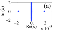
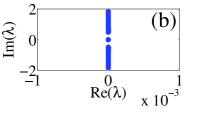
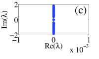
Figure 2: (Color online) Stability spectrum for solitary waves shown in Fig. 1 obtained via the linear-stability eigenvalue problem (23). The parameters used here are the same of Fig. 1.

In Figs. 1(a)-1(d) we show the profiles of the localized solutions $|\psi|^{2}$ for the cases given by Eqs. (20) and (21), in the absence of modulation (The values chosen by us for the nonlinearities are such that the norm of the solution approaches $1$). Note that we choose three ranges of values for the nonlinearities, namely, $g_{2}<0$ and $g_{3}<0$ (both self-focusing in Fig. 1(b)), $g_{2}<0$ and $g_{3}>0$ (competing type-1 in Fig. 1(c)), and $g_{2}>0$ and $g_{3}<0$ (competing type-2 in Figs. 1(a) and 1(d)). Also, we show in Figs. 2(a)-2(d) the linear stability analysis corresponding to the cases presented in Figs.1(a)-1(d), where we display the real and imaginary parts of the eigenvalue given by Eq. (23). Note that if $\mathrm{Re}(\lambda)\neq 0$, one gets a linearly unstable solution (cf. Eq. (22)). In our example, the Lorentzian-type solution (Eq. (20)) is prone to be unstable while the others solutions are linearly stable. From now on, we will call the examples for those specific choices of nonlinearities presented in Figs. 1(a)-(d) by cases A, B, C, and D, respectively.

4.2 Seesaw potential

We now analyze a potential with linear modulation in $x$-coordinate and periodic modulation in $t$. So, we choose $a=1$ and $b=-\sin(\omega t)$, such that, $\alpha=0$, $\beta=\omega^{2}\sin(\omega t)$, and $\delta=0$ with a suitable adjustment of the function $\epsilon(t)$. In this case, the amplitude and phase of the solution will be given by $\rho=1$ and $\eta=\omega x\cos(\omega t)-\frac{1}{4}\omega[\cos(\omega t)\sin(\omega t)+\omega t]$, respectively. Also, one gets $\zeta=x-\sin(\omega t)$, $\tau=t$, $g_{2}=G_{2}$ and $g_{3}=G_{3}$ (constant nonlinearities), and a seesaw potential with the form

$$V=\omega^{2}x\sin(\omega t).$$

Note that the amplitude of the above potential depends on the square of oscillation frequency of the temporal modulation.

We display in Fig. 3 the analytical profiles ($|\psi|^{2}$) of the localized solutions modulated by the seesaw potential. Note that in Figs. 3(a)-3(d) we contemplate the same cases shown in Figs. 1(a)-1(d), respectively, now with modulation of a seesaw potential. We stress that in the present case, the linear stability analysis employed in the previous case do not work anymore. Then, we analyze the stability of the solutions by direct numerical simulations of the perturbed profiles (Eq. (25)). Based on the analytical solutions, we expect stable solutions when the variance in $x$ is approximately “constant”, i.e, $var(x)=\langle x^{2}\rangle-\langle x\rangle^{2}$, with $\langle\bullet\rangle=\int_{-\infty}^{\infty}\bullet|\psi(x,t)|^{2}dx$. Indeed, due to the perturbations it will only suffer small random variations.

In Figs. 4(a)-4(d) we display the variance of $x$ versus $t$. Note that we do not present the 3D profiles to avoid problems of graphical resolution because the number of oscillations up to $t=5000$, but they were taken into account everywhere. As a conclusion, the result of Fig. 4(a) shows that the unstable solution (one whose instability is shown in Fig. 2(a)) remains unstable under the present modulation. Also, those stable solutions, whose stabilities are shown in Figs. 2(b)-2(d), remain stable. We stress that all results were verified for different values of $\omega$, varying by the step $0.05$ into the range $[0,1.0]$.

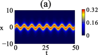
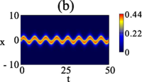
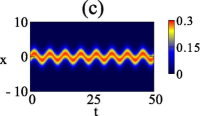
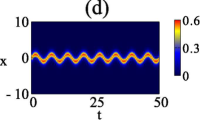
Figure 3: (Color online) Localized solutions $|\psi|^{2}$ obtained from the ansatz (2) considering $\alpha=\delta=0$ and $\beta=\omega^{2}\sin(\omega t)$ (here with $\omega=1$, for simplicity). The profiles shown in (a)-(d) corresponds to those non-modulated cases presented in Figs. 1(a)-1(d), respectively, but now with modulation. The values of the nonlinearities are the same used in Fig. 1.

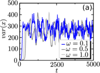
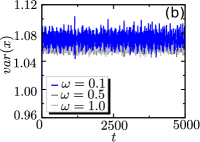
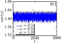
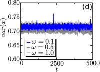
Figure 4: (Color online) Stability tests via direct numerical simulations, using the input state given by (25) with different modulation frequencies, viz. $\omega=0.1$, $0.5$, and $1.0$. We show in panels (a)-(d) the variance of $x$ versus $t$ ($var(x)$) corresponding to the cases displayed in Figs. 3(a)-3(d), respectively.

4.3 Flying-bird potential

Here we assume a quadratic modulation in $x$-coordinate with a periodic modulation in $t$-coordinate. Thus, we use $a=1+\gamma\cos(\omega t)$ (with $\gamma<1$) and $b=\epsilon=0$, getting

$$\alpha=\frac{\gamma\omega^{2}(\gamma\cos^{2}(\omega t)-\cos(\omega t)-2\gamma)}{2(\gamma\cos(\omega t)+1)^{2}},$$ (27)

$\beta=0$, and $\delta=0$. So, the amplitude and phase of the solution, the external potential and the modulated nonlinearities will be given by $\rho=\sqrt{1+\gamma\cos(\omega t)}$, $\eta=\gamma\omega x\sin(\omega t)/\{2[\gamma\cos(\omega t)+1]\}$, $V=\alpha(t)x^{2}$ (with $\alpha$ given by Eq. (27)), $g_{2}=G_{2}[1+\gamma\cos(\omega t)]^{3/2}$, and $g_{3}=G_{3}[1+\gamma\cos(\omega t)]$, respectively.

Analytical profiles of the modulated solutions are shown in Fig. 5. Note that a breathing pattern is obtained since we have nonlinearities varying harmonically while the potential presents an attractive-to-expulsive harmonic change in its profile. In Figs. 6(a)-(d) we show the time evolution of the variance of $x$ obtained by direct numerical simulations of Eq. (1). Now, differently from the variance predicted for the seesaw potential (Subsec. 4.2), here this parameter will oscillate around a constant value, which reflects the breathing pattern of the solutions.

We found different regions of stability/instability for each case. Interestingly, we observe in the case A that the Lorentzian solution becomes stable for $\omega\in[0.2,1.0]$. This behavior is observed in the results shown in Fig. 6(a), where one can see that the variance of the curve for $\omega=0.1$ increases in an unpredictable fashion while the other ones remain oscillating around a constant value. In the case B (Fig. 6(a)) we found an unstable region for $0.4\leq\omega\leq 0.55$ and the solutions remain stable outside this region. Differently form the case B, in the cases C and D (Figs. 6(c) and 6(d)) we found two unstable regions: $\omega\in[0.3,0.55]$ and $\omega=0.95$ for the case C and $\omega\in[0.25,0.65]$ and $\omega=0.75$ for the case D. Note that in the Figs. 6(b)-6(d) the variances for $\omega=0.5$ present a signature of this instability.

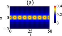
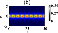
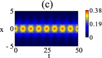
Figure 5: (Color online) Localized solutions $|\psi|^{2}$ obtained from the ansatz (2) considering $a=1+\gamma\cos(\omega t)$, $b=0$, and $\epsilon=0$. The profiles shown in (a)-(d) corresponds to the non-modulated cases presented in Figs. 1(a)-1(d), respectively, but now with modulation. The values of the nonlinearities are the same used in Fig. 1 plus $\omega=1$ and $\gamma=1/4$.

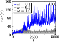
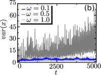
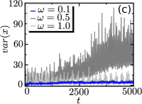
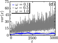
Figure 6: (Color online) Stability tests via direct numerical simulations, using the input state given by (25) with different modulation frequencies, viz. $\omega=0.1$, $0.5$, and $1.0$. We show in panels (a)-(d) the variance of $x$ versus $t$ ($var(x)$) corresponding to the cases displayed in Figs. 5(a)-5(d), respectively.

4.4 Mixed potential

In this case, we consider a mixed potential with the form $V=\alpha(t)x^{2}+\beta(t)x$, and we take $a=1+\gamma\cos(\omega t)$ and $b=-\sin(\omega t)$. We choose $\epsilon$ in a way such that $\delta=0$. The temporal modulation functions for the potential will then be written in the form:

$$\beta=\frac{\omega^{2}\sin(\omega t)[1-\gamma\cos(\omega t)]}{[1+\gamma\cos(\omega t)]^{2}},$$ (28)

with $\alpha$ given by Eq. (27). With the above choices, it is possible to check that $\rho=\sqrt{1+\gamma\cos(\omega t)}$ and $\eta=\omega x[\gamma x\sin(\omega t)+2\cos(\omega t)]/[2\gamma\cos(\omega t)+2]+\epsilon(t)$ for the amplitude and phase of the solution, respectively, and that $g_{2}=G_{2}[1+\gamma\cos(\omega t)]^{3/2}$ and $g_{3}=G_{3}[1+\gamma\cos(\omega t)]$. The modulated coordinates take the forms $\zeta=[1+\gamma\cos(\omega t)]x-\sin(\omega t)$ and $\tau=\{\gamma[4+\gamma\cos(\omega t)]\sin(\omega t)+\omega t(2+\gamma^{2})\}/2\omega$.

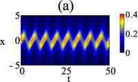
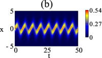
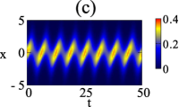
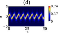
Figure 7: (Color online) Localized solutions $|\psi|^{2}$ obtained from the ansatz (2) considering $a=1+\gamma\cos(\omega t)$, $b=-\sin(\omega t)$, and $\epsilon$ in a such way that allow us to get $\delta=0$. The profiles shown in (a)-(d) corresponds to the non-modulated cases presented in Figs. 1(a)-1(d), respectively, but now with modulation. The values of the nonlinearities are the same used in Fig. 1 plus $\omega=1$ and $\gamma=1/4$.

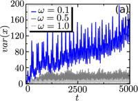
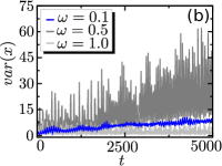
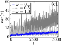
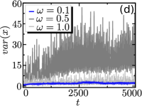
Figure 8: (Color online) Stability tests via direct numerical simulations, using the input state given by (25) with different modulation frequencies, viz. $\omega=0.1$, $0.5$, and $1.0$. We show in panels (a)-(d) the variance of $x$ versus $t$ ($var(x)$) corresponding to the cases displayed in Figs. 7 (a)-7(d), respectively.

In Figs. 7 (a)-(d) we show the analytical profiles of the modulated solutions by the mixed potential. Indeed, as expected we observe the solution oscillating around the center of the trap, in a way similar to the case of the seesaw potential, plus a breathing pattern, as in the case of the flying-bird potential. Similarly to the case of flying-bird potential, due to the breathing pattern of the mixed potential the variance of $x$ will also oscillate around a constant value. This pattern was observed in the stable solutions obtained by the numerical simulations.

The temporal evolution of variance in $x$ of the solutions are displayed in Figs. 8(a)-8(d). Specifically, for the Lorentzian solution (case A, displayed in Fig. 8(a)) the solution stabilizes for $\omega\geq 0.2$. For the cases B-D, we verify instability regions similar to those observed in the flying-bird potential, i.e., the solution loses its stability for $\omega\in[0.4,0.65]$ in case B, for $\omega\in[0.3,0.55]$ and for $\omega=0.7$ in case C, and for $\omega\in[0.25,0.55]$ and for $\omega\in[0.75,0.8]$ in case D. In fact, one can see in the example shown in Fig. 8(a) the increase in the value of the variance in $x$ for $\omega=0.1$ while for $\omega=0.5$ and $1.0$ this parameter will oscillate around a constant value. In the same way, in Figs. 8(b)-8(d) the curve of $var(x)$ with $\omega=0.5$ presents an increasing behavior illustrating the instability region mentioned above. In all cases the temporal evolution of the 3D profiles corroborate the variance behavior.

5 Summary

In this work, we investigated the NLS equation in the presence of quadratic and cubic nonlinearities that are modulated in time, under the action of a background potential modulated in space and time. We have studied two distinct solutions, constructed from Eqs. (20) and (21), and we dealt with several possibilities, with the nonlinearities being focusing or defocusing, and with the potential having four distinct features, as they appear in the subsections 4.1, 4.2, 4.3, and 4.4. The study presented several analytical solutions, showing how they can be stable or unstable, when one varies parameters that control each one of the four specific problems considered in the work.

The main results of the current study are exemplified in the eight figures that are depicted above. The four odd numbered figures illustrate solutions with vanishing potential, and with potential of the seesaw, flying-bird, or mixed type, respectively. Also, the four even figures describe the corresponding stability, which we investigated numerically. Interestingly, we see that the frequency of modulation is an important parameter to control stability of the solutions for both the self-focusing and the self-defocusing cubic nonlinearity. Among all the interesting results, we stress that the stability is not guaranteed for certain types of modulations, so the pattern of modulation can work to stabilize or destabilize the solutions.

The several investigations illustrate how to stabilize unstable solutions and how to accomplish this possibility in a diversity of scenarios. Thus, from the experimental point of view one can, for example, stabilize an unstable solution, like the one shown in Fig. 2a, with an appropriate choice of the pattern of modulation, and with a specific choice in the frequency of modulation, which is the key parameter here. In this sense, the above results encourage us to study other models, with other types of nonlinearities and solutions. We hope to report on this in the near future.

References

References

- [1] Agrawal GP. Nonlinear Fiber Optics. Academic Press. Academic Press; 2013. Available from: https://books.google.com.br/books?id=xNvw-GDVn84Chttps://books.google.com.br/books?id=b5S0JqHMoxAC.
- [2] Flach S, Willis CR. Discrete breathers. Phys Rep. 1998 mar;295(5):181–264. Available from: http://linkinghub.elsevier.com/retrieve/pii/S0370157397000689.
- [3] Andersen JD, Kenkre VM. Self-trapping and time evolution in some spatially extended quantum nonlinear systems: Exact solutions. Phys Rev B. 1993 may;47(17):11134–11142. Available from: http://link.aps.org/doi/10.1103/PhysRevB.47.11134.
- [4] Peyrard M, Dauxois T, Hoyet H, Willis CR. Biomolecular dynamics of DNA: statistical mechanics and dynamical models. Phys D Nonlinear Phenom. 1993 sep;68(1):104–115. Available from: http://linkinghub.elsevier.com/retrieve/pii/016727899390035Y.
- [5] Scott A. Nonlinear Science: Emergence and Dynamics of Coherent Structures. Oxford texts in applied and engineering mathematics. Oxford University Press; 2003. Available from: https://books.google.com.br/books?id=PkxK9AVQ6SgC.
- [6] Drazin PG, Johnson RS. Solitons: An Introduction. Cambridge Computer Science Texts. Cambridge University Press; 1989. Available from: https://books.google.com.br/books?id=HPmbIDk2u-gC.
- [7] Remoissenet M. Waves Called Solitons: Concepts and Experiments. Springer Berlin Heidelberg; 2013. Available from: https://books.google.com.br/books?id=qULtCAAAQBAJ.
- [8] Eilenberger G. Solitons: Mathematical Methods for Physicists. Springer Series in Solid-State Sciences. Springer Berlin Heidelberg; 2012. Available from: https://books.google.com.br/books?id=YKvrCAAAQBAJ.
- [9] Pethick CJ, Smith H. Bose-Einstein Condensation in Dilute Gases. Cambridge University Press; 2002.
- [10] Pitaevskii LP, Stringari S. Bose-Einstein Condensation. International Series of Monographs on Physics. Clarendon Press; 2003. Available from: https://books.google.com.br/books?id=rIobbOxC4j4C.
- [11] Malomed BA. Nonlinear Schrödinger Equations. In: Encycl. Nonlinear Sci. Taylor and Francis; 2006. p. 639–643. Available from: https://books.google.com.br/books?id=KC7gZmIEAiwC.
- [12] Buryak A. Optical solitons due to quadratic nonlinearities: from basic physics to futuristic applications. Phys Rep. 2002 nov;370(2):63–235. Available from: http://linkinghub.elsevier.com/retrieve/pii/S0370157302001965.
- [13] Hayata K, Koshiba M. Prediction of unique solitary-wave polaritons in quadratic-cubic nonlinear dispersive media. J Opt Soc Am B. 1994 dec;11(12):2581. Available from: https://www.osapublishing.org/abstract.cfm?URI=josab-11-12-2581.
- [14] Fujioka J, Cortés E, Pérez-Pascual R, Rodríguez RF, Espinosa A, Malomed BA. Chaotic solitons in the quadratic-cubic nonlinear Schrödinger equation under nonlinearity management. Chaos An Interdiscip J Nonlinear Sci. 2011;21(3):033120. Available from: http://scitation.aip.org/content/aip/journal/chaos/21/3/10.1063/1.3629985.
- [15] Dalfovo F, Giorgini S, Pitaevskii LP, Stringari S. Theory of Bose-Einstein condensation in trapped gases. Rev Mod Phys. 1999 apr;71(3):463–512. Available from: http://link.aps.org/doi/10.1103/RevModPhys.71.463.
- [16] Aranson IS, Kramer L. The world of the complex Ginzburg-Landau equation. Rev Mod Phys. 2002 feb;74(1):99–143. Available from: http://link.aps.org/doi/10.1103/RevModPhys.74.99.
- [17] Akhmediev NN, Afanasjev VV, Soto-Crespo JM. Singularities and special soliton solutions of the cubic-quintic complex Ginzburg-Landau equation. Phys Rev E. 1996 jan;53(1):1190–1201. Available from: http://link.aps.org/doi/10.1103/PhysRevE.53.1190.
- [18] Mihalache D, Mazilu D, Crasovan LC, Malomed BA, Lederer F. Three-dimensional spinning solitons in the cubic-quintic nonlinear medium. Phys Rev E. 2000 jun;61(6):7142–7145. Available from: http://link.aps.org/doi/10.1103/PhysRevE.61.7142.
- [19] Avelar AT, Bazeia D, Cardoso WB. Solitons with cubic and quintic nonlinearities modulated in space and time. Phys Rev E. 2009 feb;79(2):025602. Available from: http://link.aps.org/doi/10.1103/PhysRevE.79.025602.
- [20] Cardoso WB, Avelar AT, Bazeia D. One-dimensional reduction of the three-dimenstional Gross-Pitaevskii equation with two- and three-body interactions. Phys Rev E. 2011 mar;83(3):036604. Available from: http://link.aps.org/doi/10.1103/PhysRevE.83.036604.
- [21] Alfimov GL, Konotop VV, Pacciani P. Stationary localized modes of the quintic nonlinear Schrödinger equation with a periodic potential. Phys Rev A. 2007 feb;75(2):023624. Available from: http://link.aps.org/doi/10.1103/PhysRevA.75.023624.
- [22] Reyna AS, de Araújo CB. Nonlinearity management of photonic composites and observation of spatial-modulation instability due to quintic nonlinearity. Phys Rev A. 2014 jun;89(6):063803. Available from: http://link.aps.org/doi/10.1103/PhysRevA.89.063803.
- [23] Salasnich L, Parola A, Reatto L. Effective wave equations for the dynamics of cigar-shaped and disk-shaped Bose condensates. Phys Rev A. 2002 apr;65(4):043614. Available from: http://link.aps.org/doi/10.1103/PhysRevA.65.043614.
- [24] Salasnich L, Parola A, Reatto L. Condensate bright solitons under transverse confinement. Phys Rev A. 2002 oct;66(4):043603. Available from: http://link.aps.org/doi/10.1103/PhysRevA.66.043603.
- [25] Mateo AM, Delgado V. Effective mean-field equations for cigar-shaped and disk-shaped Bose-Einstein condensates. Phys Rev A. 2008 jan;77(1):013617. Available from: http://link.aps.org/doi/10.1103/PhysRevA.77.013617.
- [26] Adhikari SK, Salasnich L. Effective nonlinear Schrödinger equations for cigar-shaped and disc-shaped Fermi superfluids at unitarity. New J Phys. 2009 feb;11(2):023011. Available from: http://stacks.iop.org/1367-2630/11/i=2/a=023011?key=crossref.206d6a141e90aff3fffa0cee8a11aa07.
- [27] Cardoso WB, Zeng J, Avelar AT, Bazeia D, Malomed BA. Bright solitons from the nonpolynomial Schrödinger equation with inhomogeneous defocusing nonlinearities. Phys Rev E. 2013 aug;88(2):025201. Available from: http://link.aps.org/doi/10.1103/PhysRevE.88.025201.
- [28] Couto HLC, Cardoso WB. Dynamics of the soliton-sound interaction in the quasi-one-dimensional Munoz-Mateo–Delgado equation. J Phys B At Mol Opt Phys. 2015 jan;48(2):025301. Available from: http://stacks.iop.org/0953-4075/48/i=2/a=025301?key=crossref.94b619bdc9e8159b1e066778aa3ab2d4.
- [29] Biswas A, Milović D. Optical solitons with log-law nonlinearity. Commun Nonlinear Sci Numer Simul. 2010 dec;15(12):3763–3767. Available from: http://linkinghub.elsevier.com/retrieve/pii/S1007570410000523.
- [30] Calaça L, Avelar AT, Bazeia D, Cardoso WB. Modulation of localized solutions for the Schrödinger equation with logarithm nonlinearity. Commun Nonlinear Sci Numer Simul. 2014 sep;19(9):2928–2934. Available from: http://linkinghub.elsevier.com/retrieve/pii/S1007570414000550.
- [31] Soto-Crespo JM, Wright EM, Akhmediev NN. Recurrence and azimuthal-symmetry breaking of a cylindrical Gaussian beam in a saturable self-focusing medium. Phys Rev A. 1992 mar;45(5):3168–3175. Available from: http://link.aps.org/doi/10.1103/PhysRevA.45.3168.
- [32] Stepić M, Kip D, Hadžievski L, Maluckov A. One-dimensional bright discrete solitons in media with saturable nonlinearity. Phys Rev E. 2004 jun;69(6):066618. Available from: http://link.aps.org/doi/10.1103/PhysRevE.69.066618.
- [33] Melvin TRO, Champneys AR, Kevrekidis PG, Cuevas J. Radiationless Traveling Waves in Saturable Nonlinear Schrödinger Lattices. Phys Rev Lett. 2006 sep;97(12):124101. Available from: http://link.aps.org/doi/10.1103/PhysRevLett.97.124101.
- [34] Yang J. Nonlinear Waves in Integrable and Nonintegrable Systems. Society for Industrial and Applied Mathematics; 2010. Available from: http://epubs.siam.org/doi/book/10.1137/1.9780898719680.
- [35] Wang L, Li M, Qi FH, Xu T. Modulational instability, nonautonomous breathers and rogue waves for a variable-coefficient derivative nonlinear Schrödinger equation in the inhomogeneous plasmas. Phys Plasmas. 2015 mar;22(3):032308. Available from: http://scitation.aip.org/content/aip/journal/pop/22/3/10.1063/1.4915516.
- [36] Theis M, Thalhammer G, Winkler K, Hellwig M, Ruff G, Grimm R, et al. Tuning the Scattering Length with an Optically Induced Feshbach Resonance. Phys Rev Lett. 2004 sep;93(12):123001. Available from: http://link.aps.org/doi/10.1103/PhysRevLett.93.123001.
- [37] Belmonte-Beitia J, Pérez-García VM, Vekslerchik V, Konotop VV. Localized Nonlinear Waves in Systems with Time- and Space-Modulated Nonlinearities. Phys Rev Lett. 2008 apr;100(16):164102. Available from: http://link.aps.org/doi/10.1103/PhysRevLett.100.164102.
- [38] Yan Z, Konotop VV. Exact solutions to three-dimensional generalized nonlinear Schrödinger equations with varying potential and nonlinearities. Phys Rev E. 2009 sep;80(3):036607. Available from: http://link.aps.org/doi/10.1103/PhysRevE.80.036607.
- [39] Yan Z, Hang C. Analytical three-dimensional bright solitons and soliton pairs in Bose-Einstein condensates with time-space modulation. Phys Rev A. 2009 dec;80(6):063626. Available from: http://link.aps.org/doi/10.1103/PhysRevA.80.063626.
- [40] Avelar AT, Bazeia D, Cardoso WB. Modulation of breathers in the three-dimensional nonlinear Gross-Pitaevskii equation. Phys Rev E. 2010 nov;82(5):057601. Available from: http://link.aps.org/doi/10.1103/PhysRevE.82.057601.
- [41] Cardoso WB, Avelar AT, Bazeia D. Bright and dark solitons in a periodically attractive and expulsive potential with nonlinearities modulated in space and time. Nonlinear Anal Real World Appl. 2010 oct;11(5):4269–4274. Available from: http://linkinghub.elsevier.com/retrieve/pii/S1468121810000805.
- [42] Cardoso WB, Avelar AT, Bazeia D. Modulation of breathers in cigar-shaped Bose–Einstein condensates. Phys Lett A. 2010 jun;374(26):2640–2645. Available from: http://linkinghub.elsevier.com/retrieve/pii/S0375960110004895.
- [43] Cardoso WB, Avelar AT, Bazeia D, Hussein MS. Solitons of two-component Bose-Einstein condensates modulated in space and time. Phys Lett A. 2010 may;374(23):2356–2360. Available from: http://linkinghub.elsevier.com/retrieve/pii/S0375960110004068.
- [44] Serkin VN, Hasegawa A, Belyaeva TL. Nonautonomous matter-wave solitons near the Feshbach resonance. Phys Rev A. 2010 feb;81(2):023610. Available from: http://link.aps.org/doi/10.1103/PhysRevA.81.023610.
- [45] Serkin VN, Hasegawa A, Belyaeva TL. Solitary waves in nonautonomous nonlinear and dispersive systems: nonautonomous solitons. J Mod Opt. 2010 aug;57(14-15):1456–1472. Available from: http://www.tandfonline.com/doi/abs/10.1080/09500341003624750.
- [46] Zhang JF, Tian Q, Wang YY, Dai CQ, Wu L. Self-similar optical pulses in competing cubic-quintic nonlinear media with distributed coefficients. Phys Rev A. 2010 feb;81(2):023832. Available from: http://link.aps.org/doi/10.1103/PhysRevA.81.023832.
- [47] Yan Z. Nonautonomous "rogons" in the inhomogeneous nonlinear Schrödinger equation with variable coefficients. Phys Lett A. 2010 jan;374(4):672–679. Available from: http://linkinghub.elsevier.com/retrieve/pii/S0375960109014625.
- [48] He JR, Li HM. Analytical solitary-wave solutions of the generalized nonautonomous cubic-quintic nonlinear Schrödinger equation with different external potentials. Phys Rev E. 2011 jun;83(6):066607. Available from: http://link.aps.org/doi/10.1103/PhysRevE.83.066607.
- [49] He Jd, Zhang Jf, Zhang My, Dai Cq. Analytical nonautonomous soliton solutions for the cubic–quintic nonlinear Schrödinger equation with distributed coefficients. Opt Commun. 2012 mar;285(5):755–760. Available from: http://linkinghub.elsevier.com/retrieve/pii/S0030401811012302.
- [50] Dai CQ, Wang YY, Tian Q, Zhang JF. The management and containment of self-similar rogue waves in the inhomogeneous nonlinear Schrödinger equation. Ann Phys (N Y). 2012 feb;327(2):512–521. Available from: http://linkinghub.elsevier.com/retrieve/pii/S0003491611001898.
- [51] Cardoso WB, Avelar AT, Bazeia D. Modulation of localized solutions in a system of two coupled nonlinear Schrödinger equations. Phys Rev E. 2012 aug;86(2):27601. Available from: http://link.aps.org/doi/10.1103/PhysRevE.86.027601.
- [52] Arroyo Meza LE, de Souza Dutra A, Hott MB. Wide localized solitons in systems with time- and space-modulated nonlinearities. Phys Rev E. 2012 aug;86(2):026605. Available from: http://link.aps.org/doi/10.1103/PhysRevE.86.026605.
- [53] Yomba E, Zakeri GA. Solitons in a generalized space- and time-variable coefficients nonlinear Schrödinger equation with higher-order terms. Phys Lett A. 2013 dec;377(42):2995–3004. Available from: http://linkinghub.elsevier.com/retrieve/pii/S0375960113008098.
- [54] He JR, Yi L, Li HM. Localized nonlinear waves in combined time-dependent magnetic–optical potentials with spatiotemporally modulated nonlinearities. Phys Lett A. 2013 nov;377(34-36):2034–2040. Available from: http://linkinghub.elsevier.com/retrieve/pii/S0375960113006014.
- [55] Zhong WP, Belić MR, Huang T. Periodic soliton solutions of the nonlinear Schrödinger equation with variable nonlinearity and external parabolic potential. Opt - Int J Light Electron Opt. 2013 aug;124(16):2397–2400. Available from: http://linkinghub.elsevier.com/retrieve/pii/S0030402612006948.
- [56] He JR, Yi L. Formations of n-order two-soliton bound states in Bose–Einstein condensates with spatiotemporally modulated nonlinearities. Phys Lett A. 2014 mar;378(16-17):1085–1090. Available from: http://linkinghub.elsevier.com/retrieve/pii/S0375960114001303.
- [57] Soloman Raju T. Dynamics of self-similar waves in asymmetric twin-core fibers with Airy–Bessel modulated nonlinearity. Opt Commun. 2015 jul;346:74–79. Available from: http://linkinghub.elsevier.com/retrieve/pii/S0030401815001157.
- [58] Temgoua DDE, Kofane TC. Nonparaxial rogue waves in optical Kerr media. Phys Rev E. 2015 jun;91(6):063201. Available from: http://link.aps.org/doi/10.1103/PhysRevE.91.063201.
- [59] Yang Y, Yan Z, Mihalache D. Controlling temporal solitary waves in the generalized inhomogeneous coupled nonlinear Schrödinger equations with varying source terms. J Math Phys. 2015 may;56(5):053508. Available from: http://scitation.aip.org/content/aip/journal/jmp/56/5/10.1063/1.4921641.
- [60] Kumar De K, Goyal A, Raju TS, Kumar CN, Panigrahi PK. Riccati parameterized self-similar waves in two-dimensional graded-index waveguide. Opt Commun. 2015 apr;341:15–21. Available from: http://linkinghub.elsevier.com/retrieve/pii/S0030401814011444.
- [61] Meza LEA, Dutra AdS, Hott MB, Roy P. Wide localized solutions of the parity-time-symmetric nonautonomous nonlinear Schrödinger equation. Phys Rev E. 2015 jan;91(1):013205. Available from: http://link.aps.org/doi/10.1103/PhysRevE.91.013205.
- [62] Rajaraman R. Solitons and Instantons: An Introd. to Solitons and Instantons in Quantum Field Theory. North-Holland; 1987. Available from: https://books.google.com.br/books?id=r-HCoAEACAAJ.
- [63] Avelar AT, Bazeia D, Cardoso WB, Losano L. Lump-like structures in scalar-field models in dimensions. Phys Lett A. 2009 dec;374(2):222–227. Available from: http://linkinghub.elsevier.com/retrieve/pii/S037596010901353X.
- [64] Avelar AT, Bazeia D, Losano L, Menezes R. New lump-like structures in scalar-field models. Eur Phys J C. 2008 may;55(1):133–143. Available from: http://www.springerlink.com/index/10.1140/epjc/s10052-008-0578-6http://dx.doi.org/10.1140/epjc/s10052-008-0578-6.
- [65] Muñoz Mateo A, Delgado V. Effective one-dimensional dynamics of elongated Bose-Einstein condensates. Ann Phys (N Y). 2009 mar;324(3):709–724. Available from: http://linkinghub.elsevier.com/retrieve/pii/S0003491608001516.
- [66] Sinha S, Santos L. Cold Dipolar Gases in Quasi-One-Dimensional Geometries. Phys Rev Lett. 2007 oct;99(14):140406. Available from: http://link.aps.org/doi/10.1103/PhysRevLett.99.140406.
- [67] Kartashov YV, Malomed BA, Torner L. Solitons in nonlinear lattices. Rev Mod Phys. 2011 apr;83(1):247–305. Available from: http://link.aps.org/doi/10.1103/RevModPhys.83.247.
- [68] Malomed BA. Soliton Management in Periodic Systems. Springer US; 2006. Available from: https://books.google.com.br/books?id=sr2txF_x6AgC.
- [69] Kevrekidis PG, Theocharis G, Frantzeskakis DJ, Malomed BA. Feshbach Resonance Management for Bose-Einstein Condensates. Phys Rev Lett. 2003 jun;90(23):230401. Available from: http://link.aps.org/doi/10.1103/PhysRevLett.90.230401.