Zero-dimensional limit of the two-dimensional Lugiato-Lefever equation

Abstract

We study effects of tight harmonic-oscillator confinement on the electromagnetic field in a laser cavity by solving the two-dimensional Lugiato-Lefever (2D LL) equation, taking into account self-focusing or defocusing nonlinearity, losses, pump, and the trapping potential. Tightly confined (quasi-zero-dimensional) optical modes (pixels), produced by this model, are analyzed by means of the variational approximation, which provides a qualitative picture of the ensuing phenomena. This is followed by systematic simulations of the time-dependent 2D LL equation, which reveal the shape, stability, and dynamical behavior of the resulting localized patterns. In this way, we produce stability diagrams for the expected pixels. Then, we consider the LL model with the vortical pump, showing that it can produce stable pixels with embedded vorticity (vortex solitons) in remarkably broad stability areas. Alongside confined vortices with the simple single-ring structure, in the latter case the LL model gives rise to stable multi-ring states, with a spiral phase field. In addition to the numerical results, a qualitatively correct description of the vortex solitons is provided by the Thomas-Fermi approximation.

I Introduction

The Lugiato-Lefever (LL) equation LL in one and two dimensions (1D and 2D) is a fundamental model governing the dynamics of optical fields in pumped lossy laser cavities with the intrinsic Kerr nonlinearity, which may have self-focusing or defocusing sign. This equation is well known as an important tool for the analysis of pattern formation, with various applications in nonlinear optics patterns-early ; pixel . The progress in theoretical and experimental studies has recently drawn a great deal of renewed interest to the use of the LL equation in diverse settings patterns-2 -NJP . A natural extension of these studies is incorporation of external potentials into the LL equation, which can be easily fabricated in laser cavities as transverse landscapes of the refractive-index inhomogeneity, and may be used as an efficient means for the control of optical fields Kestas .

One of essential applications of the LL equation is its use for modeling well-localized pixels (i.e., sharply bounded bright spots) in the cavity pixel . In most cases, pixels are considered as anti-dark solitons, i.e., bright objects created on top of a uniformly pumped background field. In this work, we aim to demonstrate a possibility to create completely localized robust pixels (i.e., bright solitons with zero background), by adding to the model a confining potential corresponding to an isotropic 2D harmonic oscillator. Furthermore, we demonstrate that the same setting makes it possible to create stable vortex pixels, by applying a vortically structured pump. The consideration reported below combines an analytical approach, chiefly based on the variational and Thomas-Fermi approximations (VA and TFA), and systematic direct simulations, in imaginary and real time alike, with the purpose to create confined modes and test their stability.

The paper is organized as follows. The model, based on the 2D LL equation with the harmonic-oscillator trapping potential, is formulated in Section II. Analytical treatment, which makes use of the VA, power-balance equation, and TFA, is presented in Section III. Numerical results for the existence and stability of the fundamental (zero-vorticity) and vortical trapped modes are reported in Sections IV and V, respectively. The latter section also reports simple analytical results for the vortex states, obtained by means of the TFA. The paper is concluded by Section VI.

II The model

The 2D LL equation for the amplitude $\phi(x,y,t)$ of the electromagnetic field in a pumped lossy laser cavity is (see, e.g., Ref. Kestas )

$$i\left(\gamma+\frac{\partial}{\partial t}\right)\phi=\left[-\frac{1}{2}\left(\frac{\partial^{2}}{\partial x^{2}}+\frac{\partial^{2}}{\partial y^{2}}\right)+\Delta\right.$$

$$+\left.\frac{\Omega^{2}}{2}(x^{2}+y^{2})+\sigma|\phi|^{2}\right]\phi+E\;,$$ (1)

where $E$ is the pump field, $\gamma>0$ the dissipation rate, $\Delta\gtrless 0$ detuning of the pump with respect to the cavity, and $\Omega^{2}$ the strength of the confining potential, while $\sigma=-1$ and $+1$ correspond to the self-focusing and defocusing nonlinearity, respectively. By means of rescaling, one may fix $\gamma=1$, although it may be convenient to keep $\gamma$ as a free parameter, as shown below.

Stationary solutions to Eq. (1) have a simple asymptotic form at $r\equiv\sqrt{x^{2}+y^{2}}\rightarrow\infty$:

$$\phi(r)\approx-\frac{2E}{\left(\Omega r\right)^{2}}+\frac{4\left(\Delta-i\gamma\right)E}{\left(\Omega r\right)^{4}}.$$ (2)

We also note that the following exact power-balance equation ensues from Eq. (1):

$$\frac{dP}{dt}=-2\gamma P-2\int\int\mathrm{Im}\{E^{\ast}\phi(x,y,t)\}dxdy,$$ (3)

where power $P$ (alias norm) of the solitary wave is defined as

$$P=\int\int|\phi(x,y,t)|^{2}dxdy.$$ (4)

The objective is to reduce the 2D LL equation (1) to a quasi-zero-dimensional limit (a dynamical system for a pixel, similar to those realized by theoretically predicted pixel and experimentally created NJP spatial solitons) in the case of tight confinement, represented by large $\Omega^{2}$. First, we do it by means of the VA, defining

$$\phi(x,y,t)\equiv\Phi(x,y,t)\exp\left(-\gamma t\right),$$ (5)

and thus casting Eq. (1) in the form of

$$i\frac{\partial}{\partial t}\Phi = \left[-\frac{1}{2}\left(\frac{\partial^{2}}{\partial x^{2}}+\frac{\partial^{2}}{\partial y^{2}}\right)+\Delta\right.$$ (6)

$$+ \left.\frac{\Omega^{2}}{2}(x^{2}+y^{2})+\sigma e^{-2\gamma t}|\Phi|^{2}\right]\Phi+Ee^{\gamma t}.$$

Unlike the original LL equation (1), the transformed one (6) can be directly derived from a real time-dependent Lagrangian,

$$L = \int\int dxdy\left\{\frac{i}{2}\left(\Phi_{t}^{\ast}\Phi-\Phi^{\ast}\Phi_{t}\right)+\frac{1}{2}\left(|\Phi_{x}|^{2}+|\Phi_{y}|^{2}\right)\right.$$ (7)

$$+ \left[\Delta+\frac{\Omega^{2}}{2}(x^{2}+y^{2})\right]|\Phi|^{2}+\frac{\sigma}{2}e^{-2\gamma t}\,|\Phi|^{4}$$

$$+ \left.e^{\gamma t}\left(E\Phi^{\ast}+E^{\ast}\Phi\right)\right\}\,.$$

III Analytical considerations

III.1 The variational approximation

For the 1D LL equation without trapping potentials, the VA was developed in Ref. VA-LL . To derive this approximation in a form appropriate for the present model, we note that, in the lowest approximation, Eq. (6) gives rise to the following asymptotic form of solutions at $r\rightarrow\infty$: $\Phi=-2E\left(\Omega r\right)^{-2}e^{\gamma t}$, cf. Eq. (2). This form suggests us to adopt an ansatz based on the fractional expression, with real variables $f(t)$ and $\chi(t)$, which may be combined into a complex one, $F(t)=f(t)\exp\left(i\chi(t)\right)$:

$$\Phi\left(x,y,t\right) = -\frac{2E}{\Omega^{2}}e^{\gamma t}\frac{F(t)}{1+r^{2}F(t)}\equiv\epsilon\,e^{\gamma t}\frac{f(t)\,e^{i\chi(t)}}{1+r^{2}f(t)\,e^{i\chi(t)}}\;,\quad$$ (8)

$$\epsilon \equiv -\frac{2E}{\Omega^{2}}\;.$$ (9)

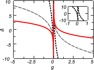
Figure 1: (Color online) Lines in the parameter plane of ($\Delta$, $g$), along which solutions of the overdetermined system (27), (28) exist. Here, solid red, dashed gray, and dotted black lines correspond, respectively, to $\Omega=2$, $4$, and $6$. The inset displays a zoom of the curve for $\Omega=10$.

The insertion of ansatz (8) in Eq. (7) and subsequent integration gives rise to an effective Lagrangian,

$$\frac{e^{-2\gamma t}}{\pi\epsilon^{2}}L_{\mathrm{eff}} = \frac{1}{2}fq_{1}(\chi)\frac{d\chi}{dt}-\frac{1}{2}q_{2}(\chi)\sin\chi\frac{df}{dt}+f^{2}q_{2}(\chi)$$ (10)

$$+ \Delta fq_{1}(\chi)+\frac{\sigma\epsilon^{2}}{8}f^{3}q_{3}(\chi)-\Omega^{2}q_{1}(\chi)\cos\chi$$

$$- \frac{\Omega^{2}}{4}\int d\chi[q_{3}(\chi)\sin\chi]\,,$$

with $q_{1}(\chi)\equiv\chi/\sin\chi$, $q_{2}(\chi)\equiv[\left(\sin\chi-\chi\cos\chi\right)/\sin^{3}\chi$, and $q_{3}(\chi)\equiv[2\chi-\sin\left(2\chi\right)]/\sin^{3}\chi$. The last term in Eq. (10) is cast in the integral form as a result of “renormalization”: the respective term in the original Lagrangian formally diverges logarithmically at $R\rightarrow\infty$, but the diverging part actually does not depend on $f$ and $\chi$, and it may be cancelled by means of the differentiation with respect to $\chi$ and subsequent integration, also with respect to $\chi$.

The Euler-Lagrange equations following from Lagrangian (10) are (taking into account that the Lagrangian must be substituted into the action, $\int Ldt$, and then the action must be subjected to the variation; this makes it necessary to apply the time differentiation to $e^{2\gamma t}$):

$$\frac{1}{2}\left[q_{2}(\chi)\cos\chi+q_{2}^{\prime}(\chi)\sin\chi+q_{1}(\chi)\right]\frac{df}{dt}$$ (11)

$$+ \left(\gamma f-\Omega^{2}\sin\chi\right)q_{1}(\chi)+\left(\Omega^{2}\cos\chi-\Delta\,f\right)q_{1}^{\prime}(\chi)$$

$$- f^{2}\,q_{2}^{\prime}(\chi)-\frac{g}{8}f^{3}q_{3}^{\prime}(\chi)+\frac{\Omega^{2}}{4}q_{3}(\chi)\sin\chi=0\;,$$

$$\Delta q_{1}(\chi)+2\,f\,q_{2}(\chi)+\frac{3g}{8}\,f^{2}\,q_{3}(\chi)+\gamma q_{2}(\chi)\sin\chi$$ (12)

$$+ \frac{1}{2}\left[q_{2}(\chi)\cos\chi+q_{2}^{\prime}(\chi)\sin\chi+q_{1}(\chi)\right]\frac{d\chi}{dt}=0\;,$$

where a renormalized nonlinearity coefficient is [see Eq. (9)]

$$g=\sigma\epsilon^{2}\equiv 4\sigma E^{2}/\Omega^{4}.$$ (13)

Note that, although it may seem that Eqs. (11) and (12) are singular at $\chi=0$, in reality all the singularities cancel. A singularity is instead possible at $\chi=\pi$.

We consider stationary (fixed-point) solutions of Eqs. (11) and (12) by setting $df/dt=d\chi/dt=0$, which yields

$$\left(\Omega^{2}\sin\chi-\gamma f\right)q_{1}(\chi)+\left(\Delta\,f-\Omega^{2}\cos\chi\right)q_{1}^{\prime}(\chi)$$ (14)

$$+ f^{2}\,q_{2}^{\prime}(\chi)+\frac{g}{8}f^{3}q_{3}^{\prime}(\chi)-\frac{\Omega^{2}}{4}q_{3}(\chi)\sin\chi=0,$$

$$\Delta q_{1}(\chi)+2\,f\,q_{2}(\chi)+\frac{3g}{8}\,f^{2}\,q_{3}(\chi)+\gamma q_{2}(\chi)\sin\chi=0.$$ (15)

Further, it is possible to find approximate solutions of Eqs. (14) and (15), assuming that they have

$$|\chi|\ll\pi~{}.$$ (16)

In this case, Eq. (15), in the first approximation, assumes the form of

$$\Delta+\frac{2}{3}f+\frac{g}{2}f^{2}+\frac{\gamma}{3}\chi=0.$$ (17)

Similarly, in the lowest approximation Eq. (14) yields an expression for $\chi$:

$$\chi=\frac{30\gamma f}{10\Omega^{2}+f\left[10\Delta+8f+3gf^{2}\right]}\;,$$ (18)

The assumption (16) may be then secured by a natural assumption of the strong confinement, i.e., considering large values of $\Omega$. In this case, Eqs. (17) and (18) can be further simplified to

$$f \approx \frac{-2\pm\sqrt{4-18g\Delta}}{3g},$$ (19)

$$\chi \approx \frac{\gamma\left(-2\pm\sqrt{4-18g\Delta}\right)}{g\Omega^{2}}.$$ (20)

Obviously, Eqs. (19) and (20) produce a physically relevant result under condition $g\Delta<2/9$.

One can construct another approximate solution for large detuning $\Delta$:

$$f \approx \sqrt{-2\Delta/g}-2/\left(3g\right),$$ (21)

$$\chi \approx (15/2)\gamma/\Delta.$$ (22)

In the general case, stationary solutions of Eqs. (14) and (15), where, as said above, we may fix $\gamma=1$, depend on three parameters: $\Delta\gtrless 0$, $g\gtrless 0$ [see Eq. (13)], and $\Omega^{2}>0$.

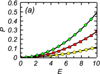
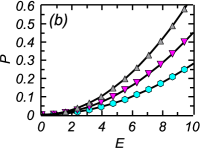
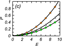
Figure 2: (Color online) Power $P$ versus pumping strength $E$. Variational results for the defocusing case ($\sigma=+1$), produced by simplified equations (19) and (20), are shown in (a), with $g=1$, by curves with circles (yellow), boxes (red), and diamonds (green), for $\Delta=-1$, $-4$, and $-10$, respectively. The self-focusing case ($\sigma=-1$) is shown in (b), with $g=-1$, by curves with hexagons (cyan), down triangles (magenta), and up triangles (gray), for $\Delta=1$, $4$, and $10$, respectively. In (c) we compare the analytical and numerical results for the defocusing case ($g=1$ and $\Delta=-10$), shown, severally, by curves with diamonds (green) and stars (orange), and analytical results for the self-focusing case [$g=-1$ and $\Delta=10$, shown by the curve with up triangles (gray)]. The solutions numerically found in the case of the self-focusing are unstable. In all the plots, $\Omega=10$ and $\gamma=1$ are fixed here.

In addition to the consideration of the stationary solutions (fixed points), the full dynamical version of the VA, based on Eqs. (11) and (12), can be also used to analyze their stability, as well as evolution of unstable solutions. However, in practical terms such a dynamical analysis turns out to be quite cumbersome, direct numerical simulations being actually more efficient, as shown below.

III.2 The power-balance condition

The substitution of ansatz (8) in the definition of power (4) and power-balance equation (3) yields

$$P = \frac{4\pi E^{2}f}{\Omega^{4}}\frac{\chi}{\sin(\chi)},$$ (23)

$$\frac{dP}{dt} = -\frac{8\pi\gamma E^{2}f}{\Omega^{4}}\frac{\chi}{\sin(\chi)}+\frac{4\pi E^{2}}{\Omega^{2}}\chi,$$ (24)

(in these expressions, $f>0$ is implied). Equation (24) predicts the equilibrium condition, $dP/dt=0$, at

$$\sin(\chi)=\frac{2\gamma}{\Omega^{2}}f.$$ (25)

Note that $E$ drops out from Eq. (25), and condition $\sin(\chi)\leq 1$, following from Eq. (25), imposes a restriction on $f$,

$$f\leq\Omega^{2}/(2\gamma).$$ (26)

Finally, for $|\chi|\ll\pi$ Eq. (25) simplifies to $\chi\approx\left(2\gamma/\Omega^{2}\right)f$. Using this to eliminate $f$ in favor of $\chi$, Eqs. (17) and (18) give rise to the following system of equations:

$$\frac{g\Omega^{4}\chi^{3}}{80\gamma^{3}}+\frac{\Omega^{2}\chi^{2}}{15\gamma^{2}}+\frac{\Delta\chi}{6\gamma}-\frac{1}{6} = 0,$$ (27)

$$\frac{g\Omega^{4}\chi^{2}}{8\gamma^{2}}+\frac{1}{3\gamma}\left(\Omega^{2}+\gamma^{2}\right)\chi+\Delta = 0.$$ (28)

Of course, the system of two equations (27) and (28) for the single unknown $\chi$ is overdetermined, and a solution of this system may exist only if a special restriction is imposed on parameters, as shown in Fig. 1, in the plane of ($\Delta$, $g$), for $\gamma=1$ and three different fixed values of the confinement strength, $\Omega=2$, $\Omega=4$, and $\Omega=10$. Note that these curves do not depend on the pumping strength, $E$. Indeed, this parameter is related only to the power of the solution, see Eq. (23) and Fig. 2. The meaning of the overdetermined system is that, realizing the VA and power-balance condition simultaneously, its solution has a better chance to produce an accurate approximation. This expectation is qualitatively corroborated below, see Fig. 9 and related text in the next section.

Generic properties of the modes predicted by ansatz (8) are characterized by the corresponding dependence of power $P$ on the pumping strength, $E$. Using, for this purpose, the simplified approximation given by Eqs. (19) and (20), we display the dependences for the defocusing nonlinearity ($g=1$) in Fig. 2(a), at fixed values of the detuning, $\Delta=-1$, $-4$, and $-10$. Figure 2(b) displays the same dependences in the case of the self-focusing nonlinearity ($g=-1$), for $\Delta=1$, $4$, and $10$. Note that power $P$ is not symmetric with respect to the reversal of the signs of nonlinearity $g$ and detuning $\Delta$.

In Fig. 2(c) we compare the VA results for the self-defocusing ($g=1$ and $\Delta=-10$) and focusing ($g=-1$ and $\Delta=10$) cases. In addition, Fig. 2(c) includes full numerical results (for details see the next Section). It is seen that the simplified VA produces a qualitatively correct prediction, which is not quite accurate quantitatively. Below, we demonstrate that the VA is completely accurate only in small black regions shown in Fig. 9.

III.3 The Thomas-Fermi approximation (TFA)

In the case of the self-defocusing sign of the nonlinearity, and positive mismatch, $\Delta>0$, the ground state, corresponding to a sufficiently smooth stationary solution of Eq. (1), $\phi=\phi(r)$, may be produced by the TFA, which neglects derivatives in the radial equation TFA :

$$\left(\Delta-i\gamma+\frac{\Omega^{2}}{2}r^{2}+\sigma|\phi|^{2}\right)\phi=-E\;.$$ (29)

In particular, the TFA is relevant if $\Delta$ is large enough.

The TFA-produced equation (29) for the ground-states’s configuration is not easy to solve analytically, as it is a cubic algebraic equation with complex coefficients. The situation greatly simplifies in the limit case of a very large mismatch, viz., $\Delta\gg\gamma$ and $\Delta^{3}\gg\sigma E^{2}$. Then, both the imaginary and nonlinear terms may be neglected in Eq. (29), to yield

$$\phi(r)\approx-E\left(\Delta+\frac{\Omega^{2}}{2}r^{2}\right)^{-1}.$$ (30)

This simple approximation, which may be considered as a limit form of ansatz (8), can be used to produce estimates for various characteristics of the ground state (see, in particular, Fig. 5 below). In fact, the TFA will be the most relevant tool in Section V, as an analytical approximation for trapped vortex modes, for which the use of the VA, even in its stationary form, is too cumbersome.

The TFA cannot be applied to nonstationary solutions, hence it does not provide direct predictions for stability of stationary modes. However, it usually tends to produce ground states, thus predicting stable solutions. This expectation is corroborated by results produced below.

IV Numerical results for fundamental modes

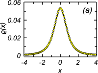
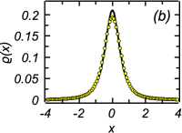
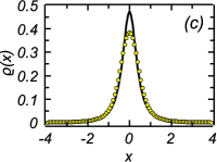
Figure 3: (Color online) Profiles of fundamental trapped modes, $\varrho(x)$, obtained via imaginary-time simulations of Eq. (1), are shown by yellow circles. Black solid lines display counterparts of the same profiles produced by the variational approximation based on ansatz (8). The parameters are (a) $\Delta=-1$, (b) $\Delta=-4$, (c) $\Delta=-10$, others fixed as $\Omega=10$, $\gamma=1$, $E=10$, and $g=1$ (the self-defocusing nonlinearity).

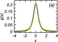
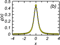
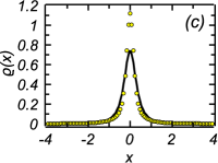
Figure 4: (Color online) The same as in Fig. 3, for parameters (a) $\Delta=1$, (b) $\Delta=4$, (c) $\Delta=10$, with $\Omega=10$, $\gamma=1$, $E=10$, and $g=-1$ (the self-focusing nonlinearity).

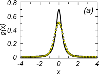
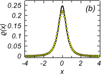
Figure 5: (Color online) Following Figs. 3 and 4, chains of yellow circles depict profiles of fundamental trapped modes, $\varrho(x)$, obtained via imaginary-time simulations of Eq. (1), for the self-defocusing nonlinearity, $g=1$, and large positive values of the mismatch: $\Delta=10$ in (a) and $\Delta=20$ in (b). Black solid lines display the same profiles, as produced by the simplest version of the Thomas-Fermi approximation, given by Eq. (32). Other parameters are $\Omega=10$, $\gamma=1$, and $E=10$.

IV.1 Stationary trapped modes

To obtain accurate results, and verify the validity of the VA predictions which are presented in the previous section, we here report results obtained as numerical solutions of Eq. (1). First, we aim to find ground-state localized states by means of imaginary-time propagation. In the framework of this method, one numerically integrates Eq. (1), replacing $t$ by $-it$ and normalizing the solution at each step of the time integration to maintain a fixed total power IT . For testing stability of stationary states, Eq. (1) was then simulated in real time, by means of the fourth-order split-step method implemented in a GNU Octave program Eaton_Octave (for a details concerning the method and its implementations in MATLAB, see Ref. Yang_10 ).

In Fig. 3 we show 1D integrated intensity profiles $\varrho(x)$, defined as

$$\varrho(x)\equiv\int_{-\infty}^{+\infty}|\phi(x,y)|^{2}dy,$$ (31)

and obtained from the imaginary-time solution of Eq. (1), along with their analytical counterparts produced by the VA based on Eq. (8), for three different values of detuning $\Delta$, viz., (a) $\Delta=-1$, (b) $\Delta=-4$, and (c) $\Delta=-10$, for $g=1$ (the self-defocusing nonlinearity) and $\Omega=10$ and $E=10$. We used Eqs. (19) and (20) to produce values of the parameters $f$ and $\chi$ in ansatz (8), which was then used as the initial guess in direct numerical simulations.

In Fig. 4 we display results similar to those shown in Fig. 3, but for the self-focusing nonlinearity ($g=-1$) and three different (positive) values of $\Delta$, viz., (a) $\Delta=1$, (b) $\Delta=4$, and (c) $\Delta=10$, with fixed $\Omega=10$ and $E=10$. In both cases of $g=\pm 1$, the VA profiles show good match to the numerical ones, although the accuracy slightly deteriorates with the increase of $|\Delta|$.

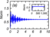
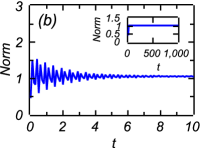
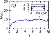
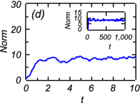
Figure 6: (Color online) The evolution of the norm [total power (4)] of the solution starting from ansatz (8) perturbed by $5\%$ random noise, as produced by real-time simulations of Eq. (1). Here the results are presented for the defocusing nonlinearity, i.e., $g=1$, with (a) $\Delta=-1$ and (b) $\Delta=-10$, and for the focusing nonlinearity, i.e., $g=-1$, with (c) $\Delta=1$ and (d) $\Delta=10$. Other parameters are $E=10$, $\Omega=10$, and $\gamma=1$. The evolution of the norm at large times is shown in the insets.

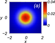
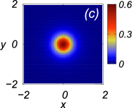
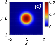
Figure 7: (Color online) Density profile $|\phi|^{2}$ obtained via direct numerical simulations of Eq. (1) in the case of the self-defocusing nonlinearity ($g=1$). Inputs, represented by ansatz (8) with the addition of $5\%$ random noise, are displayed in panels (a) for $\Delta=-1$ and (c) for $\Delta=-10$. The corresponding profiles produced by the simulations at $t=1000$ are shown in (b) and (d), respectively. Other parameters are the same as in Fig. 6.

Note that the results displayed in Fig. 4, for the situations to which the TFA does not apply, because the nonlinearity is self-focusing in this case, demonstrate  the growth of the maximum value, $\varrho(x=0)$, with the increase of mismatch $\Delta$. In the case of self-defocusing it is natural to expect decay of $\varrho_{\mathrm{TFA}}(x=0)$ with the increase of $\Delta$. As shown in Fig. 5, this expectation is confirmed by the numerical results and the TFA alike. In particular, for the integrated intensity profile defined by Eq. (31), the simplest version of the TFA, produced by Eq. (30), easily gives

$$\varrho_{\mathrm{TFA}}(x)=\frac{2\pi E^{2}}{\Omega^{4}}\left(\frac{2\Delta}{\Omega^{2}}+x^{2}\right)^{-3/2}.$$ (32)

Figure 5 also corroborates that the TFA, even in its simplest form, becomes quite accurate for sufficiently large values of $\Delta>0$.

IV.2 Stability of the stationary modes

The stability of the trapped configurations predicted by ansatz (8) was tested in real-time simulations of Eq. (1), adding $5\%$ random noise to the input. We display the results, showing the evolution of the solution’s norm (total power) in the case of the defocusing nonlinearity ($g=1$), for $\Delta=-1$ and $-10$, in Figs. 6(a) and (b), respectively. The insets show the asymptotic behavior at large times. In the case of the defocusing nonlinearity, the solution quickly relaxes to a numerically exact stationary form, and remains completely stable at $t>10$ (in fact, real-time simulations always quickly converge to stable solutions at all values of the parameters). However, in the case of the self-focusing with $\Omega=10$, the solutions are unstable, suffering rapid fragmentation, as seen in Fig. 8. This behavior is also exemplified in results shown in Figs. 6(c) and 6(d) for the temporal evolution of the solution’s total power in the case of the self-focusing nonlinearity ($g=-1$), for $\Delta=1$ and for $\Delta=10$, respectively. The instability of the fundamental modes in this case is a natural manifestation of the modulational instability in the LL equation MI . Note that the large size of local amplitudes in small spots, which is attained in the course of the development of the instability observed in Fig. 8, implies the trend to the onset of the 2D collapse driven by the self-focusing cubic nonlinearity collapse .

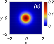
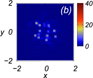
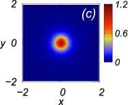
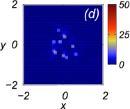
Figure 8: (Color online) The same as in Fig. 7, but in the case of the self-focusing nonlinearity ($g=-1$). Panels (a,b) and (c,d) are drawn for $\Delta=1$ and $\Delta=10$, respectively. Here, the profiles shown in (b) and (d) are outputs of the simulations obtained at $t=10$.

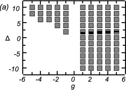
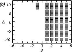
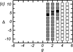
Figure 9: The existence area of stable modes obtained by means of real-time simulation of Eq. (1). To generate the area, we used the input in the form of ansatz (8) with parameters predicted by the VA, adding random noise at the $5\%$ amplitude level. We here consider (a) $\Omega=2$, (b) $\Omega=4$, and (c) $\Omega=10$. In all the cases, the norm (total power) of the solution undergoes variations. For parameter values corresponding to the gray boxes it stabilizes after a short relaxation period. In the white boxes, the norm keeps oscillating, while the solution maintains the localized profile, avoiding onset of instability. The simulations in the region not covered by boxes feature instability scenarios: in the case of $g\leq 0$ the solution suffers fragmentation, like in Figs. 8(b) and 8(d)), while in the case of self-defocusing the solution is subject to fragmentation due to the strong nonlinearity [e.g., at $g>5$ in (c)]. In the black region, the output states are very close to the input. Other parameters are $E=10$, and $\gamma=1$. The data for the linear system, corresponding to $g=0$, are not included, as in the linear system all the stationary solutions are obviously stable.

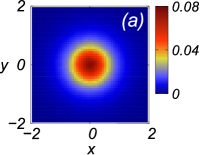
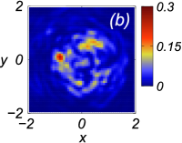
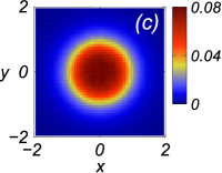
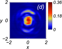
Figure 10: (Color online) The same as in Fig. 8, but for $g=10$. Panels (a,b) and (c,d) pertain to $\Delta=-10$ and $\Delta=10$, respectively. The unstable output profiles are displayed at $t=10$.

In Figs. 7 and 8 we display the time evolution of density profiles $|\phi|^{2}$ produced by the simulations of Eq. (1) with the self-defocusing and focusing nonlinearity, respectively. The input profiles are again taken as per the VA ansatz (8) with the addition of $5\%$ random noise. In Figs. 7(a) and 7(c) we show the perturbed input profiles in the case of self-defocusing, for $\Delta=-1$ and $\Delta=-10$, respectively, while the corresponding profiles at $t=1000$ are displayed in Figs. 7(b) and 7(d). Note that the agreement between the variational and numerical profiles tends to deteriorate with the increase of $|\Delta|$ [the same trend as observed in Fig. 2(c)].

Further, in Figs. 8(a) and 8(c) we display the perturbed input profiles in the case of the self-focusing nonlinearity for $\Delta=1$ and $\Delta=10$, respectively, with the corresponding profiles at $t=1000$ displayed in Figs. 8(b) and 8(d). These results clearly confirm the instability of the perturbed solutions, as suggested by the evolution of the total power depicted in Figs. 6(c) and 6(d). Strong instability is observed for all values of $g<0$, which corresponds to the self-focusing.

The findings for the existence and stability of the localized pixels are summarized by diagrams displayed in Fig. 9. To produce them, we analyzed the temporal evolution of total power (4), parallel to monitoring the spatial profile of each solution at large times ($t=100$ and $t=1000$). In Fig. 9, we address three different values of strength $\Omega$ of the trapping potential: (a) $\Omega=2$, (b) $\Omega=4$, and (c) $\Omega=10$. The stability area is represented by gray and white boxes, which correspond, respectively, to robust static outputs and those which feature small residual oscillations, while the parameter area not covered by boxes corresponds to unstable solutions. This includes the area of $g\leq 0$ (self-focusing), where the modes suffer strong instability observed in Figs. 8(b) and 8(d) at $\Omega=10$, but may be stable at $\Omega=2$ and $4$ [in the latter case, the stability domain for $g>0$ is very small, as seen in Fig. 9(b)]. On the other hand, at $g>5$ and $\Omega=10$, the solution undergoes fragmentation under the action of the strong self-defocusing nonlinearity, for all values of $-10\leq\Delta\leq+10$. An example of that is displayed in Fig. 10 for $g=10$ and two extreme values of the mismatch, $\Delta=-10$ and $+10$.

In the stability area, black spots highlight values of the parameters at which the output profiles of the static solutions, observed at $t=1000$, are very close to the respective input profiles, i.e., the VA provides very accurate predictions. Generally, the shape of the stability area in the form of the vertical stripe, observed in Fig. 9(c), roughly follows the vertical direction of the dotted black line in Fig. 1, which pertains to the same value of $\Omega=10$. On the other hand, the expansion of the stability area in the horizontal direction for $\Omega=2$ and $\Omega=4$, which is observed in Figs. 9(a,b), qualitatively complies with the strong change of the curves in Fig. 1 for the same values of $\Omega$. Looking at Fig. 9, one can also conclude that large positive values of $\Delta$ help to additionally expand the stability region.

We stress that the results shown in Fig. 9 are extremely robust: real-time simulations lead to them, even starting with zero input. The input provided by the VA ansatz (8) is used above to explore the accuracy of the VA, which is relevant, as similar approximations can be applied to similar models, incorporating the pump, linear loss, and Kerr nonlinearity (self-defocusing or focusing).

V Vortex solitons

V.1 Analytical considerations: the Thomas-Fermi approximation

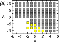
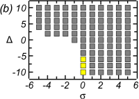
Figure 11: (Color online) The stability area in the plane of ($\Delta$, $\sigma$) for vortex solutions numerically generated by real-time simulations of Eq. (1) with vortex pump (33). Other parameters are $\Omega=2$, $\gamma=1$, and (a) $E_{0}=1$ or (b) $E_{0}=2$. Simple stable vortices are found in the gray area, while the yellow one represents stable modes with the spiral phase structure which features a full turn, and a multi-ring radial structure, see a typical example in Fig. 14. No stable vortices were found in the white area.

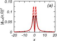
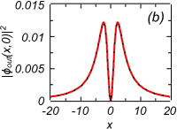
Figure 12: (Color online) Output profiles $|\phi_{\mathrm{out}}(x,0)|^{2}$ of stable ring-shaped vortices, produced by real-time integration of Eq. (1) with pump profile (33), for two different values of $|\sigma|$ (the absolute value of the nonlinearity coefficient). The radial shapes obtained with the self-defocusing ($\sigma=5$) and focusing ($\sigma=-5$) nonlinearities are displayed by solid black and dashed red lines, respectively, for $\Delta=0$ (a) and $\Delta=10$ (b). Other parameters are $\gamma=1$, $\Omega=2$ and $E_{0}=1$.

In the previous sections, we considered uniform pump field $E$, which generates fundamental modes without vorticity. Here we explore the confined LL model with space-dependent pump carrying the vorticity. It is represented by the driving term

$$E=E_{0}re^{i\theta}$$ (33)

in Eq. (1), where $\theta$ is the angular coordinate and $E_{0}=\mathrm{const}$. This term naturally corresponds to the pump supplied by a vortex laser beam (with vorticity $1$) vortex beam . In the case of multiple vorticity $m>1$ (which will be considered elsewhere), Eq. (33) is replaced by $E=E_{0}r^{m}e^{im\theta}$.

Patterns supported by the vortex pump correspond to factorized solutions of the stationary version of Eq. (1), taken as

$$\phi\left(r,\theta\right)=e^{i\theta}A(r),$$ (34)

with complex amplitude $A$ satisfying the following radial equation:

$$\left[\frac{1}{2}\left(\frac{d^{2}}{dr^{2}}+\frac{1}{r}\frac{d}{dr}-\frac{1}{r^{2}}\right)-\Delta+i\gamma-\frac{\Omega^{2}}{2}r^{2}-\sigma|A|^{2}\right]A=$$

$$E_{0}r\;.$$ (35)

As an analytical approximation, the TFA for vortex solitons may be applied here, cf. Ref. TFA-vortex . In the general case, the TFA implies dropping the derivatives in the radial equation, which leads to a complex cubic equation for $A$, cf. Eq. (29), under the conditions $\sigma>0$ (self-defocusing) and $\Delta>0$ (positive mismatch):

$$\left[\Delta-i\gamma+\frac{1}{2}\left(\frac{1}{r^{2}}+\Omega^{2}r^{2}\right)+\sigma|A|^{2}\right]A=-E_{0}r\;.$$ (36)

Equation (36), as well as its counterpart (29) for the zero-vorticity states, strongly simplifies in the limit of large $\Delta>0$, when both the imaginary and and nonlinear terms may be neglected:

$$A(r)=-E_{0}r\left[\Delta+\frac{1}{2}\left(\frac{1}{r^{2}}+\Omega^{2}r^{2}\right)\right]^{-1}.$$ (37)

In particular, the simplest approximation provided by Eq. (37) makes it possible to easily predict the radial location of maximal intensity in the ring-shaped vortex mode:

$$r_{\max}^{2}=\left(\sqrt{\Delta^{2}+3\Omega^{2}}+\Delta\right)/\Omega^{2}.$$ (38)

Comparison of values given by Eq. (38) with their counterparts extracted from numerically found vortex-ring shapes, which are displayed below in Figs. 12(a) and (b) for $\Delta\geq 0$, demonstrates that the analytically predicted values are smaller than the numerical counterparts by $11\%$ for $\Delta=0$, and by $6\%$ for $\Delta=10$. Naturally, the TFA provides better accuracy for large $\Delta,$ but even for $\Delta=0$ the prediction is reasonable. Furthermore, Eq. (37) predicts a virtually exact largest intensity, $\left|A(r=r_{\max})\right|^{2}$, for the small-amplitude mode displayed in Fig. 12(b).

V.2 Numerical results

Equation (1) with vortex pump profile (33) was numerically solved with zero input. This simulation scenario is appropriate, as vortex states, when they are stable, are sufficiently strong attractors to draw solutions developing from the zero input.

The results, produced by systematic real-time simulations, are summarized in Fig. 13 for $\Omega=2$ in Eq. (1) and $E_{0}=1$ or $2$ in Eq. (33). The figure displays stability areas for the vortex modes in the plane of free control parameters ($\Delta$, $\sigma)$ (the mismatch and nonlinearity strength). It is worthy to note that the stability domain for the self-focusing nonlinearity ($\sigma<0$) is essentially larger than in the diagram for the fundamental (zero-vorticity) modes, which is displayed, also for $\Omega=2$, in Fig. 9. This fact may be naturally explained by the fact that the vanishing of the vortex drive (33) at $r\rightarrow 0$, in the combination with the intrinsic structure of the vortex states, makes the central area of the pattern nearly “empty”, thus preventing the onset of the modulational instability in it.

In the gray areas in Fig. 11, the stable vortex modes have a simple ring-shaped structure, with typical radial profiles shown in Fig. 12. In the case of zero mismatch, $\Delta=0$ [Fig. 11(a)], the vortex state naturally acquires a higher amplitude under the action of the self-focusing. On the other hand, in the case of large positive mismatch [Fig. 11(b)], the small amplitude is virtually the same under the action of the focusing and defocusing, which is explained, as mentioned above, by the TFA that reduces to Eq. (37).

In unstable (white) areas in Fig. 11, direct simulations lead to quick fragmentation of vortically driven patterns into small spots, that feature a trend to developing the above-mentioned critical collapse collapse . A typical example of the unstable evolution is displayed in Fig. 13.

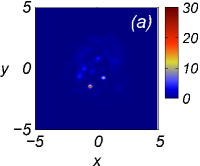
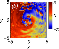
Figure 13: (Color online) (a) Local-intensity $|\phi\left(x,y\right)|^{2}$ and (b) phase profiles of an unstable pattern, produced by the simulations of Eq. (1) with vortex pump (33) and the strong self-focusing ($\sigma=-5$) at $t=20$. Other parameters are $\Delta=-8$, $\gamma=1$, $\Omega=2$, and $E_{0}=1$.

More sophisticated stable vortex profiles are observed in yellow areas in Fig. 13. They are characterized by a multi-ring radial structure, and a spiral shape of the vorticity-carrying phase distribution, as shown in Fig. 14. The yellow areas are defined as those in which the spiral phase field performs a full turn by $360$ degrees, as can be seen in Fig. 14(b). Note that this area exists for both the focusing and defocusing signs of the nonlinearity in Fig. 13(a), and solely for zero nonlinearity in Fig. 13(b), which corresponds to the stronger pump.

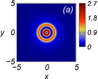
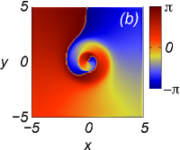
Figure 14: (Color online) A stable multi-ring vortex with the spiral phase field. Panels (a), (b), and (c) display, respectively, the 2D local-intensity pattern, phase field, and the radial structure. Parameters are the same as in Fig. 13, except for a weaker self-focusing strength, $\sigma=-1$.

The spiral shape of the phase pattern is explained by the fact that radial amplitude $A(r)$ in solution (34) is a complex function, as is explicitly shown, in particular, by Eqs. (2) and (36). The spirality of vortices is a well-known feature of 2D complex Ginzburg-Landau equations GL . However, unlike the present situation, the spirality is not usually related to a multi-ring radial structure. Patterns with multi-ring shapes usually exist as excited states, on top of stable ground states in the same models, being unstable to azimuthal perturbations Javid . For this reason, the stability of complex modes, like the one displayed in Fig. 14, is a noteworthy finding.

Lastly, a typical example of a stable vortex at the boundary between the simple (non-spiral) and complex (spiral-shaped) ones is presented in Fig. 15. It features emerging spirality in the phase field, but the radial structure keeps the single-ring shape.

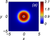
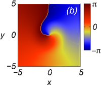
Figure 15: (Color online) The same as in Fig. 13, but with the self-defocusing sigh of the nonlinearity, $\sigma=2$.

VI Conclusion

We have introduced the 2D model based on the LL (Lugiato-Lefever) equation with confinement imposed by the harmonic-oscillator trap. In spite of the action of the uniform pump, the confinement creates well localized patterns, which may be used for the creation of robust small-area pixels in applications. The VA (variational approximation), based on a novel fractional ansatz, as well as a simple TFA (Thomas-Fermi approximation), were elaborated to describe the fundamental (zero-vorticity) confined modes. The VA effectively reduces the 2D LL equation to the zero-dimensional version. The VA is additionally enhanced by taking into regard the balance condition for the integral power. The comparison with the full numerical analysis has demonstrated that the VA provides qualitatively accurate predictions, which are also quantitatively accurate, in some areas of the parameter space. The systematic numerical analysis has produced overall stability areas for the confined pattern in the underlying parameter space, which demonstrate that the patterns tend to be less stable and more stable under the action of the self-focusing and defocusing nonlinearity, respectively (although very strong self-defocusing causes fragmentation of the patterns). The increase of the confinement strength leads to shrinkage of the stability area, although it does not make all the states unstable. On the other hand, large positive values of the cavity’s detuning tends to expand the region of the stability in the parameter space.

We have also explored vortex solitons (which may be used to realize vortical pixels in microcavities) supported by the pump with embedded vorticity. In this case, the simple TFA provides a qualitatively correct description, and systematically collected numerical results reveal a remarkably large stability area in the parameter space, for both the self-defocusing and focusing signs of the nonlinearity. In addition to simple vortices, stable complex ones, featuring the multi-ring radial structure and the spiral phase field, have been found too. As an extension of the present work, a challenging issue is to look for confined states with multiple embedded vorticity.

A summary of authors’ contributions to the work: the numerical part has been carried out by W.B.C. Analytical considerations were chiefly performed by B.A.M. and L.S. All the authors have contributed to drafting the text of the paper.

- (1) L. A. Lugiato and R. Lefever, Spatial dissipative structures in passive optical systems, Phys. Rev. Lett. 58, 2209-2211 (1987).
- (2) G.-L. Oppo, M. Brambilla, and L. A. Lugiato, Formation and evolution of roll patterns in optical parametric oscillators, Phys. Rev. A 49, 2028-2032 (1994).
- (3) M. Brambilla, L. A. Lugiato, F. Prati, L. Spinelli, and W. J. Firth, Spatial soliton pixels in semiconductor devices, Phys. Rev. Lett. 79, 2042 (1997).
- (4) L. Gelens, D. Gomila, G. Van der Sande, J. Danckaert, P. Colet, and M. A. Matías, Dynamical instabilities of dissipative solitons in nonlinear optical cavities with nonlocal materials, Phys. Rev. A 77, 033841 (2008); T. Miyaji, I. Ohnishi,and Y. Tsutsumi, Bifurcation analysis to the Lugiato-Lefever equation in one space dimension, Physica D 239, 2066-2083 (2010); K. Panajotov, D. Puzyrev, A. G. Vladimirov, S. V. Gurevich, and M. Tlidi, Impact of time-delayed feedback on spatiotemporal dynamics in the Lugiato-Lefever model, Phys. Rev. A 93, 043835 (2016).
- (5) G. J. de Valcárcel and K. Staliunas, Phase-bistable Kerr cavity solitons and patterns, Phys. Rev. A 87, 043802 (2013).
- (6) P. Parra-Rivas, D. Gomila, M. A. Matías, S. Coen, and L. Gelens, Dynamics of localized and patterned structures in the Lugiato-Lefever equation determine the stability and shape of optical frequency combs, Phys. Rev. A 89, 043813 (2014); C. Godey, I. V. Balakireva, A. Coillet, Aurelien, and Y. K. Chembo, Stability analysis of the spatiotemporal Lugiato-Lefever model for Kerr optical frequency combs in the anomalous and normal dispersion regimes, ibid. 89, 063814 (2014); T. Hansson and S. Wabnitz, Frequency comb generation beyond the Lugiato-Lefever equation: multi-stability and super cavity solitons, J. Opt. Soc. Am. B 32, 1259-1266 (2015); F. Copie, M. Conforti, A. Kudlinski, and A. Mussot, and S. Trillo, Competing Turing and Faraday instabilities in longitudinally modulated passive resonators, Phys. Rev. Lett. 116, 143901 (2016); P. Parra-Rivas, E. Knobloch, D. Gomila, and L. Gelens, Dark solitons in the Lugiato-Lefever equation with normal dispersion, Phys. Rev. A 93, 063839 (2016).
- (7) J. K. Jang, M. Erkintalo, K. Luo, G.-L. Oppo, S. Coen, and S. G. Murdoch, Controlled merging and annihilation of localised dissipative structures in an AC-driven damped nonlinear Schrödinger system, New J. Phys. 18, 0336034 (2016).
- (8) A. B. Matsko and L. Maleki, On timing jitter of mode locked Kerr frequency combs, Opt. Exp. 21, 28862 (2013).
- (9) L. P. Pitaevskii and A. Stringari, Bose-Einstein Condensation (Clarendon Press, Oxford, 2003).
- (10) E. Cerboneschi, R. Mannella, E. Arimondo, and L. Salasnich, Oscillation frequencies for a Bose condensate in a triaxial magnetic trap, Phys. Lett. A 249, 495-5000 (1998); M. L. Chiofalo, S. Succi, and M. P. Tosi, Ground state of trapped interacting Bose-Einstein condensates by an explicit imaginary-time algorithm, Phys. Rev. E 62, 7438 (2000); X. Antoine, W. Baoc, and C. Besse, Computational methods for the dynamics of the nonlinear Schrödinger/Gross–Pitaevskii equations, Comp. Phys. Commun. 184, 2621 (2013).
- (11) J. W. Eaton, D. Bateman, and S. Hauberg, GNU Octave Manual - Version 3 (Network Theory Ltd., UK, 2008).
- (12) J. Yang, Nonlinear waves in integrable and nonintegrable systems (SIAM, Philadelphia, USA, 2010).
- (13) S. Coen, H. G. Randle, S. Thibaut, and M. Erkinalo, Modeling of octave-spanning Kerr frequency combs using a generalized mean-field Lugiato-Lefever model, Opt. Lett. 38, 37 (2013); C. Godey, I. V. Balakireva, A. Coillet, and Y. K. Chembo, Stability analysis of the spatiotemporal Lugiato-Lefever model for Kerr optical frequency combs in the anomalous and normal dispersion regimes, Phys. Rev. A 89, 063814 (2014); T. Hansson and S. Wabnitz, Dynamics of microresonator frequency comb generation: models and stability, Nanophotonics 5, 231 (2016).
- (14) L. Bergé, Wave collapse in physics: Principles and applications to light and plasma waves, Phys. Rep. 303, 259 (1998); G. Fibich, The Nonlinear Schrödinger Equation: Singular Solutions and Optical Collapse (Springer: Heidelberg, 2015).
- (15) L. Allen, M. W. Beijersbergen, R. J. C. Spreeuw, and J. P. Woerdman, Orbital angular momentum of light and the transformation of Laguerre-Gaussian laser modes, Phys. Rev. A 45, 8185 (1992); I. V. Basistiy, V. Yu. Bazhenov, M. S. Soskin, and M. V. Vasnetsov, Optics of light beams with screw dislocations, Opt. Commun. 103, 422 (1993); S. Franke-Arnold, L. Allen, and M. Padgett, Advances in optical angular momentum, Laser & Photon. Rev. 2, 299 (2008).
- (16) L. Salasnich, A. Parola, and L. Reatto, Bosons in a toroidal trap: Ground state and vortices, Phys. Rev. A 59, 2990 (1999); A. L. Fetter, Rotating trapped Bose-Einstein condensates, Rev. Mod. Phys. 81, 647 (2009); L. Salasnich and B.A. Malomed, Solitons and solitary vortices in pancake-shaped Bose-Einstein condensates, Phys. Rev. A 79, 053620 (2009); R. Driben, Y. V. Kartashov, B. A. Malomed, T. Meier, and L. Torner, Soliton gyroscopes in media with spatially growing repulsive nonlinearity, Phys. Rev. Lett. 112, 020404 (2014); J. Qin, G. Dong, and B. A. Malomed, Stable giant vortex annuli in microwave-coupled atomic condensates, Phys. Rev. A 94, 053611 (2016).
- (17) T. Bohr, G. Huber, and E. Ott, The structure of spiral-domain patterns and shocks in the 2D complex Ginzburg-Landau equation, Physica D 106, 95 (1997); M. Gabbay, E. Ott, and P. N. Guzdar, The dynamics of scroll wave filaments in the complex Ginzburg-Landau equation, ibid. 118, 371 (1998); L.-C. Crasovan, B. A. Malomed, and D. Mihalache, Stable vortex solitons in the two-dimensional Ginzburg-Landau equation, Phys. Rev. E 63, 016605 (2001); D. Mihalache, D. Mazilu, F. Lederer, Y. V. Kartashov, L.-C. Crasovan, L. Torner, and B. A. Malomed, Stable vortex tori in the three-dimensional cubic-quintic Ginzburg-Landau equation, Phys. Rev. Lett. 97, 073904 (2006).
- (18) J. Atai, Y. J. Chen, and J. M. Soto-Crespo, Stability of 3-dimensional self-trapped beams with a dark spot surrounded by bright rings of varying intensity, Phys. Rev. A 49, R3170 (1994); A. Dubietis,G. Tamosauskas, G. Fibich, and B. Ilan, Multiple filamentation induced by input-beam ellipticity, Opt. Lett. 29, 1126 (2004).