THERMODYNAMICS OF THE FERMI GAS IN A NANOTUBE

Abstract

For the ideal Fermi gas that fills the space inside a cylindrical tube, there are calculated the thermodynamic characteristics in general form for arbitrary temperatures, namely: the thermodynamic potential, energy, entropy, equations of state, heat capacities and compressibilities. All these quantities are expressed through the introduced standard functions and their derivatives. The radius of the tube is considered as an additional thermodynamic variable. It is shown that at low temperatures in the quasi-one-dimensional case the temperature dependencies of the entropy and heat capacities remain linear. The dependencies of the entropy and heat capacities on the chemical potential have sharp maximums at the points where the filling of a new discrete level begins. The character of dependencies of thermodynamic quantities on the tube radius proves to be qualitatively different in the cases of fixed linear and fixed total density. At the fixed linear density these dependencies are monotonous and at the fixed total density they have an oscillating character.
Key words: Fermi particle, nanotube, thermodynamic functions, low-dimensional systems, equation of state, heat capacity, compressibility

I Introduction

The model of the ideal Fermi gas is the basis for understanding the properties of electron and other many-fermion systems. In many cases it is also possible to describe with reasonable accuracy the behavior of systems of interacting Fermi particles within the approximation of an ideal gas of quasiparticles whose dispersion law differs from the dispersion law of free particles. It is essential that thermodynamic characteristics of the ideal Fermi gas at arbitrary temperatures in the volume case can be expressed through the special Fermi functions, and thus it is possible to obtain and verify all relations of the phenomenological thermodynamics on the basis of the quantum microscopic model.

In recent time, much attention has been paid to investigation of low-dimensional systems, in particular of properties of the Fermi gas in nanotubes and quantum wells, because apart from purely scientific interest the study of such objects is rather promising for the solid-state electronics Ando ; Komnik ; DNG ; Vagner ; Freik ; SP . Thermodynamics relations for the Fermi gas in the confined geometry have been studied much less than in the volume case LL and require further investigation. Thermodynamic properties of the Fermi gas at arbitrary temperatures in a quasi-two-dimensional quantum well have been studied in detail by the authors in work PS . A detailed understanding of the properties of such systems must serve as a basis for the study of low-dimensional systems of interacting particles monaga ; Luttinger ; Deshpande .

It is considered that strongly correlated Fermi systems, to which also low-dimensional systems of Fermi particles are attributed, in many respects essentially differ from the usual Fermi liquid systems Landau ; PN . At that the properties of quasi-one-dimensional or quasi-two-dimensional systems are often compared with the theory of bulk Fermi liquid Landau ; PN . However, as seen even on the examples of the quasi-two-dimensional system of noninteracting particles which was considered by the authors in work PS and the quasi-one-dimensional system considered in the present work, the properties of low-dimensional systems can substantially differ, especially at low temperatures, from the properties of the bulk system owing to the quantum size effect. For this reason, the theory of Fermi liquid itself in conditions of the confined geometry must, generally speaking, be formulated differently than in the volume case.

The consideration of low-dimensional models of interacting Fermi particles leads to a conclusion about unique properties of such systems monaga ; Luttinger ; Deshpande . It should be kept in mind, however, that real systems are always three-dimensional and their low dimensionality manifests itself only in the boundedness of motion of particles in one, two or three coordinates.

In considering statistical properties of the three-dimensional many-particle systems one usually passes in results to the thermodynamic limit, setting in final formulas the volume and number of particles to infinity at the fixed density. It is of general theoretical interest to study the statistical properties of many-particle systems in which one or two dimensions remain fixed, and the thermodynamic limiting transition is carried out only over remaining coordinates. In this case the coordinates, over which the thermodynamic limiting transition is not performed, should be considered as additional thermodynamic variables. The model of the ideal Fermi gas allows to build the thermodynamics of low-dimensional systems based on the statistical treatment.

In the present work, the thermodynamics of the ideal Fermi gas that fills the space inside a cylindrical tube is studied. There are calculated its thermodynamic characteristics in general form for arbitrary temperatures, namely: the thermodynamic potential, energy, entropy, equations of state, heat capacities and compressibilities. All these quantities are expressed through the standard functions introduced in the work and their derivatives. It is suggested the representation of thermodynamic quantities in the dimensionless “reduced” form, which is convenient owing to the fact that it does not contain geometric dimensions of the system. The case of low temperatures and tubes of small radius is studied more in detail. It is shown that at low temperatures in the quasi-one-dimensional case under consideration the temperature dependencies of the entropy and heat capacities remain linear, the same as in the quasi-two-dimensional PS and the volume cases Landau ; PN , except the specific points where the filling of a new discrete level begins. Moreover, the dependencies of the entropy and heat capacities on the chemical potential have sharp maximums at these points. The behavior of thermodynamic quantities with the tube radius proves to be qualitatively different, depending on whether the linear or the total density is fixed. At the fixed linear density these dependencies prove to be monotonous and at the fixed total density they have an oscillating character.

II Thermodynamics of the Fermi gas in a cylindrical tube

The model of the ideal Fermi gas is the basis for studying the bulk properties of Fermi systems of particles of different nature. In the two-dimensional case an analogous role is played by the ideal Fermi gas contained between two parallel planes, whose thermodynamics was considered in detail in PS . In this work the thermodynamics properties of the ideal Fermi gas enclosed in a cylindrical tube of radius $R$ and length $L$ are studied. The length of the tube is assumed to be macroscopic, and no restrictions are imposed on the radius of the tube. The main attention is paid to studying the properties of tubes of small radius, which corresponds to transition to the quasi-one-dimensional case, at low temperatures. It is everywhere assumed that the spin of the Fermi particle is equal to 1/2. It is also assumed that the potential barrier on the surface of the tube is infinite, so that the wave function of a particle turns into zero at the boundary. The solutions of the Schrödinger equation in this case have the form

$$\begin{array}[]{l}\displaystyle{\varphi_{k,n,\nu}(r,\alpha,z)=\frac{1}{J_{n}^{\prime}(\rho_{n\nu})R\sqrt{\pi L}}\,e^{ikz}e^{\pm in\alpha}J_{n}\left(\rho_{n\nu}\frac{r}{R}\right),}\end{array}$$ (1)

where $\rho_{n\nu}$ are the zeros of the Bessel function of the order $n$, $J_{n}(\rho_{n\nu})=0$, $n=0,1,\ldots$, $\nu=1,2,\ldots$. The energy of a particle:

$$\begin{array}[]{l}\displaystyle{\varepsilon_{k,n,\nu}=\frac{\hbar^{2}k^{2}}{2m}+\rho_{n\nu}^{2}\frac{\hbar^{2}}{2mR^{2}},}\end{array}$$ (2)

and the distribution function has the form

$$\begin{array}[]{ll}\displaystyle{f_{k,n,\nu}=\big{[}\exp\beta(\varepsilon_{k,n,\nu}-\mu)+1\big{]}^{-1},}\end{array}$$ (3)

where $\beta=1/T$ is the inverse temperature. Pay attention that the discrete energy levels with $n=0$ are nondegenerate, and the levels with $n\geq 1$ are twice degenerate in the projection of angular momentum on the $z$ axis.

Thermodynamic functions of the Fermi gas both in the volume case and in the case of lower dimensionality PS can be expressed through the Fermi function defined by the formula

$$\begin{array}[]{l}\displaystyle{\Phi_{s}(t)=\frac{1}{\Gamma(s)}\int_{0}^{\!\infty}\frac{z^{s-1}\,dz}{e^{z-t}+1},}\end{array}$$ (4)

where $s$ is an integer or half-integer positive number, $\Gamma(s)$ is the gamma function. For calculation of the bulk properties of the Fermi gas it is sufficient to know the functions (4) with half-integer indices $s=1/2,3/2,5/2$, and for the quasi-two-dimensional case – with integer indices $s=1,2$. For the quasi-one-dimensional case under consideration in this work the functions with half-integer indices $s=1/2,3/2$ are required as well.

It is convenient to introduce the dimensionless temperature $\tau\equiv T/\varepsilon_{R}$ and the dimensionless chemical potential $\eta\equiv\mu/\varepsilon_{R}$, with normalization on the energy

$$\begin{array}[]{l}\displaystyle{\varepsilon_{R}=\frac{\hbar^{2}}{2mR^{2}},}\end{array}$$ (5)

and to define the functions of these two dimensionless variables by the following relation

$$\begin{array}[]{ll}\displaystyle{\Psi_{s}(\tau,\eta)\equiv\sum_{n=0}^{\infty}\sum_{\nu=1}^{\infty}g_{n}\Phi_{s}(t_{n\nu})=\vspace{2mm}}\\ \displaystyle{\hskip 36.98857pt=\sum_{\nu=1}^{\infty}\Phi_{s}(t_{0\nu})+2\sum_{n=1}^{\infty}\sum_{\nu=1}^{\infty}\Phi_{s}(t_{n\nu}).}\end{array}$$ (6)

Here the parameter $t_{n\nu}\equiv\beta(\mu-\rho_{n\nu}^{2}\varepsilon_{R})\equiv\tau^{-1}(\eta-\rho_{n\nu}^{2})$, and the factor $g_{n}\equiv 2-\delta_{n0}$ accounts for the degeneracy order of levels. It equals unity for the levels with $n=0$ and two for the rest of the levels.

After integration over momenta the thermodynamic potential $\Omega$, number of particles $N$, energy $E$ and entropy $S$ are expressed through the functions (6)

$$\begin{array}[]{ll}\displaystyle{\Omega=-\frac{2LT}{\Lambda}\Psi_{3/2}(\tau,\eta),}\end{array}$$ (7)

$$\begin{array}[]{ll}\displaystyle{N=\frac{2L}{\Lambda}\Psi_{1/2}(\tau,\eta),}\end{array}$$ (8)

$$\begin{array}[]{ll}\displaystyle{E=\frac{LT}{\Lambda}\!\left[\Psi_{3/2}(\tau,\eta)+2\frac{\eta}{\tau}\Psi_{1/2}(\tau,\eta)+2\tau\frac{\partial\Psi_{3/2}(\tau,\eta)}{\partial\tau}\right],}\end{array}$$ (9)

$$\begin{array}[]{ll}\displaystyle{S=\frac{3L}{\Lambda}\!\left[\Psi_{3/2}(\tau,\eta)+\frac{2}{3}\,\tau\frac{\partial\Psi_{3/2}(\tau,\eta)}{\partial\tau}\right],}\end{array}$$ (10)

where $\Lambda\equiv\left(2\pi\hbar^{2}\big{/}mT\right)^{\!1/2}$ is the thermal de Broglie wavelength. The volume $n=N\big{/}\pi R^{2}L$ and the linear $n_{\!L}=N\big{/}L$ densities of particles are obviously given as

$$\begin{array}[]{ll}\displaystyle{n=\frac{2}{\pi R^{2}\Lambda}\Psi_{1/2}(\tau,\eta),\qquad n_{\!L}=\frac{2}{\Lambda}\Psi_{1/2}(\tau,\eta).}\end{array}$$ (11)

The thermodynamic potential (7) is a function of the temperature, chemical potential, the length of the tube and its radius: $\Omega=\Omega(T,\mu,L,R)$. In contrast to the volume case when $\Omega$ is proportional to the volume $V$, in this case it is proportional to the length $L$ and depends in a complicated manner on the radius $R$. This circumstance is conditioned by the evident anisotropy of the system under consideration, since here the motions along the tube and in the direction of radius are qualitatively different. In statistical mechanics it is customary to pass in the final formulas to the thermodynamic limit: $V\rightarrow\infty$, $N\rightarrow\infty$ at $n=N/V=\rm{const}$. In the present case it is more accurate to write down the thermodynamic limit somewhat differently, namely

$$\begin{array}[]{ll}\displaystyle{L\rightarrow\infty,\,N\rightarrow\infty\textrm{\,\,\,\,at\,\,\,}n_{\!L}\equiv N/L=\rm{const}.}\end{array}$$ (12)

It is thereby stressed that the transition to infinite volume occurs only owing to increasing the length of the tube, with its radius $R$ being fixed.

The differential of the thermodynamic potential (7) has the form

$$\begin{array}[]{ll}\displaystyle{d\Omega=\frac{\Omega}{L}\,dL\,-\frac{4LT}{\Lambda}\!\left[\frac{\eta}{\tau}\Psi_{1/2}+\tau\frac{\partial\Psi_{3/2}}{\partial\tau}\right]\!\frac{dR}{R}\,-\vspace{2mm}}\\ \displaystyle{\hskip 17.07164pt-\frac{2L}{\Lambda}\Psi_{1/2}\,d\mu\,-\frac{L}{\Lambda}\!\left[3\Psi_{3/2}+2\tau\frac{\partial\Psi_{3/2}}{\partial\tau}\right]\!dT.}\end{array}$$ (13)

Here it was taken into account that $\partial\Psi_{3/2}\big{/}\partial\eta=\tau^{-1}\Psi_{1/2}$ and $d\varepsilon_{R}=-(2\varepsilon_{R}/R)dR$. Naturally, the usual thermodynamic relations hold $S=-\big{(}\partial\Omega\big{/}\partial T\big{)}_{\mu,L,R}$, $N=-\big{(}\partial\Omega\big{/}\partial\mu\big{)}_{T,L,R}$, as well as $\Omega=E-TS-\mu N$.

III Pressures

In a bulk system the pressure is connected with the thermodynamical potential by the known formula $p=-\Omega/V$. In the considered quasi-one-dimensional case the system is anisotropic since the character of motion of particles along the tube and in the direction of its radius is different and, therefore, the usual formula for the pressure is invalid. The force exerted by the gas on the wall perpendicular to the $z$ axis is different from the force exerted on the side wall of the tube. These forces can be calculated in the same way as in the volume case LL . The pressures on the planes perpendicular to the $z$ axis and on the wall of the tube, on the basis of the relations $p=-(\partial E/\partial V)_{S}$ and $V=\pi R^{2}L$, are given by the formulas

$$\begin{array}[]{ll}\displaystyle{p_{\parallel}=-\frac{1}{\pi R^{2}}\!\left(\frac{\partial E}{\partial L}\right)_{\!S,R},\quad p_{R}=-\frac{1}{2\pi LR}\!\left(\frac{\partial E}{\partial R}\right)_{\!S,L},}\end{array}$$ (14)

or

$$\begin{array}[]{ll}\displaystyle{p_{\parallel}=-\frac{1}{\pi R^{2}}\!\left(\frac{\partial\Omega}{\partial L}\right)_{\!T,\mu,R},\quad p_{R}=-\frac{1}{2\pi LR}\!\left(\frac{\partial\Omega}{\partial R}\right)_{\!T,\mu,L}.}\end{array}$$ (15)

The differential of the thermodynamic potential (13) can be represented in the form

$$\begin{array}[]{ll}\displaystyle{d\Omega=-p_{\parallel}\pi R^{2}dL-p_{R}2\pi LRdR-Nd\mu-SdT.}\end{array}$$ (16)

Considering the form of the thermodynamic potential (7), we obtain the formulas determining the pressures through the functions (6):

$$\begin{array}[]{ll}\displaystyle{p_{\parallel}=\frac{2T}{\pi R^{2}\Lambda}\Psi_{3/2},\quad p_{R}=\frac{2T}{\pi R^{2}\Lambda}\!\left(\frac{\eta}{\tau}\Psi_{1/2}+\tau\frac{\partial\Psi_{3/2}}{\partial\tau}\right).}\end{array}$$ (17)

The energy is connected with the pressures by the formula

$$\begin{array}[]{ll}\displaystyle{E=\frac{1}{2}\pi R^{2}L\!\left(p_{\parallel}+2p_{R}\right),}\end{array}$$ (18)

which in the volume limit $p_{\parallel}=p_{R}=p$  turns into the known relation $pV=(2/3)E$  for the Fermi gas LL .

IV Reduced form of thermodynamic quantities

It is convenient to introduce dimensionless quantities, which we will call “reduced” and designate them by a tilde on top, for the entropy, energy, pressures, volume and linear densities:

$$\begin{array}[]{ll}\displaystyle{\tilde{S}\equiv\frac{2\pi^{1/2}}{3}\frac{R}{L}S,\qquad\tilde{E}\equiv 4\pi^{1/2}\frac{R^{3}}{L}\frac{m}{\hbar^{2}}E,\vspace{2mm}}\\ \displaystyle{\tilde{p}_{\parallel}\equiv 2\pi^{3/2}R^{5}\frac{m}{\hbar^{2}}p_{\parallel},\qquad\tilde{p}_{R}\equiv 2\pi^{3/2}R^{5}\frac{m}{\hbar^{2}}p_{R},\vspace{2mm}}\\ \displaystyle{\tilde{n}\equiv\pi^{3/2}R^{3}\,n,\qquad\tilde{n}_{\!L}\equiv\pi^{1/2}R\,n_{\!L}=\tilde{n}.}\end{array}$$ (19)

The reduced quantities are functions of only two independent dimensionless variables – the temperature $\tau$ and the chemical potential $\eta$:

$$\begin{array}[]{ll}\displaystyle{\tilde{S}=\tau^{1/2}\!\left(\Psi_{3/2}+\frac{2}{3}\,\tau\frac{\partial\Psi_{3/2}}{\partial\tau}\right),\vspace{2mm}}\\ \displaystyle{\tilde{E}=\tau^{3/2}\!\left(\Psi_{3/2}+2\frac{\eta}{\tau}\Psi_{1/2}+2\tau\frac{\partial\Psi_{3/2}}{\partial\tau}\right),\vspace{2mm}}\\ \displaystyle{\tilde{p}_{\parallel}=\tau^{3/2}\Psi_{3/2},\quad\tilde{p}_{R}=\tau^{3/2}\!\left(\frac{\eta}{\tau}\Psi_{1/2}+\tau\frac{\partial\Psi_{3/2}}{\partial\tau}\right),\vspace{2mm}}\\ \displaystyle{\tilde{n}=\tilde{n}_{\!L}=\tau^{1/2}\Psi_{1/2}.}\end{array}$$ (20)

The use of the reduces quantities is convenient owing to the fact that they do not contain explicitly geometric dimensions of the system.

V Heat capacities

An important directly measurable thermodynamic quantity is the heat capacity. In the geometry under consideration heat capacities can be defined under various conditions different from those which take place in the volume case. In order to obtain heat capacities, it is necessary to calculate the quantity $C=T(dS/dT)$. For this purpose, it is convenient to express the differential of the entropy through the reduced quantities:

$$\begin{array}[]{ll}\displaystyle{\frac{dS}{S}=\left(\frac{1}{\tilde{S}}\frac{\partial\tilde{S}}{\partial\eta}-\frac{1}{\tilde{n}_{\!L}}\frac{\partial\tilde{n}_{\!L}}{\partial\eta}\right)\!d\eta+\!\left(\frac{1}{\tilde{S}}\frac{\partial\tilde{S}}{\partial\tau}-\frac{1}{\tilde{n}_{\!L}}\frac{\partial\tilde{n}_{\!L}}{\partial\tau}\right)\!d\tau.}\end{array}$$ (21)

In the volume case at the fixed number of particles, which is assumed here, the equation of state is $p=p(T,V)$. If the chemical potential is used as an independent variable, then the equation of state is defined parametrically by the equations $p=p(T,V,\mu)$ and $N=N(T,V,\mu)$. To obtain the heat capacity as a function of only temperature, one constraint should be imposed between the pressure and the volume. In the simplest case, it its possible to fix either the volume or the pressure, thus obtaining the heat capacities $C_{V}$ and $C_{p}$.

Under given conditions, owing to anisotropy of the system, there are two equations of state (17) for two pressures $p_{R}=p_{R}(T,R,L,\mu)$ and $p_{\parallel}=p_{\parallel}(T,R,L,\mu)$, which at the fixed average number of particles should be considered together with the equation $N=N(T,R,L,\mu)$. To obtain the heat capacity as a function of only temperature, two additional constraints should be set between the pressures $p_{R},p_{\parallel}$ and the dimensions of the system $R,L$, namely $F_{1}(p_{R},p_{\parallel},R,L)=0$ and $F_{2}(p_{R},p_{\parallel},R,L)=0$. In the simplest case, two of four quantities $p_{R},p_{\parallel},R,L$ can be fixed. Then the heat capacity as a function of temperature can be considered under fixation of one of the following pairs of quantities: $(R,L)$, $(p_{R},p_{\parallel})$, $(R,p_{\parallel})$, $(R,p_{R})$, $(L,p_{\parallel})$, $(L,p_{R})$. Fixation of the first of pairs $(R,L)$ corresponds to the heat capacity at a constant volume in the volume case, and of the second $(p_{R},p_{\parallel})$ – to the heat capacity at a constant pressure. In calculations the following relations should be taken into account:

$$\begin{array}[]{ll}\displaystyle{\frac{d\tilde{n}_{\!L}}{\tilde{n}_{\!L}}=\frac{dR}{R}-\frac{dL}{L},\quad\,\,\frac{d\tau}{dT}=\frac{1}{\varepsilon_{R}}+\frac{2\tau}{R}\frac{dR}{dT}.}\end{array}$$ (22)

Finally, we obtain the formulas for the reduced heat capacities $\displaystyle{\tilde{C}\equiv\frac{2\pi^{1/2}}{3}\frac{R}{L}\,C}$ under different conditions, being valid at arbitrary temperatures:

$$\begin{array}[]{ll}\displaystyle{\tilde{C}_{LR}=\tau\!\left\{\frac{\partial\tilde{S}}{\partial\tau}-\frac{\partial\tilde{S}}{\partial\eta}\frac{\big{(}\partial\tilde{n}_{\!L}/\partial\tau\big{)}}{\big{(}\partial\tilde{n}_{\!L}/\partial\eta\big{)}}\right\},}\end{array}$$ (23)

$$\begin{array}[]{ll}\displaystyle{\tilde{C}_{p_{\parallel}p_{R}}=\tau\,\frac{\displaystyle{\left(\frac{\partial\tilde{S}}{\partial\eta}-\frac{\tilde{S}}{\tilde{n}_{\!L}}\frac{\partial\tilde{n}_{\!L}}{\partial\eta}\right)\!\!\left(\tilde{p}_{R}\frac{\partial\tilde{p}_{\parallel}}{\partial\tau}-\tilde{p}_{\parallel}\frac{\partial\tilde{p}_{R}}{\partial\tau}\right)+\!\left(\frac{\partial\tilde{S}}{\partial\tau}-\frac{\tilde{S}}{\tilde{n}_{\!L}}\frac{\partial\tilde{n}_{\!L}}{\partial\tau}\right)\!\!\left(\tilde{p}_{\parallel}\frac{\partial\tilde{p}_{R}}{\partial\eta}-\tilde{p}_{R}\frac{\partial\tilde{p}_{\parallel}}{\partial\eta}\right)}}{\displaystyle{\tilde{p}_{\parallel}\frac{\partial\tilde{p}_{R}}{\partial\eta}-\tilde{p}_{R}\frac{\partial\tilde{p}_{\parallel}}{\partial\eta}+\frac{2}{5}\,\tau\!\left(\frac{\partial\tilde{p}_{\parallel}}{\partial\eta}\frac{\partial\tilde{p}_{R}}{\partial\tau}-\frac{\partial\tilde{p}_{\parallel}}{\partial\tau}\frac{\partial\tilde{p}_{R}}{\partial\eta}\right)}},}\end{array}$$ (24)

$$\begin{array}[]{ll}\displaystyle{\tilde{C}_{Rp_{\parallel}}=\tau\!\left\{\!\left(\frac{\partial\tilde{S}}{\partial\tau}-\frac{\tilde{S}}{\tilde{n}_{\!L}}\frac{\partial\tilde{n}_{\!L}}{\partial\tau}\right)-\!\left(\frac{\partial\tilde{S}}{\partial\eta}-\frac{\tilde{S}}{\tilde{n}_{\!L}}\frac{\partial\tilde{n}_{\!L}}{\partial\eta}\right)\!\!\frac{\big{(}\partial\tilde{p}_{\parallel}/\partial\tau\big{)}}{\big{(}\partial\tilde{p}_{\parallel}/\partial\eta\big{)}}\right\},}\end{array}$$ (25)

$$\begin{array}[]{ll}\displaystyle{\tilde{C}_{Lp_{\parallel}}=\tau\,\frac{\displaystyle{\frac{\tilde{n}_{\!L}}{2}\frac{\partial\tilde{p}_{\parallel}}{\partial\eta}\!\left(\frac{\partial\tilde{S}}{\partial\tau}-\frac{\tilde{S}}{\tilde{n}_{\!L}}\frac{\partial\tilde{n}_{\!L}}{\partial\tau}\right)\!-\frac{\tilde{n}_{\!L}}{2}\frac{\partial\tilde{p}_{\parallel}}{\partial\tau}\!\left(\frac{\partial\tilde{S}}{\partial\eta}-\frac{\tilde{S}}{\tilde{n}_{\!L}}\frac{\partial\tilde{n}_{\!L}}{\partial\eta}\right)\!+\frac{5}{2}\,\tilde{p}_{\parallel}\!\left(\frac{\partial\tilde{S}}{\partial\eta}\frac{\partial\tilde{n}_{\!L}}{\partial\tau}-\frac{\partial\tilde{S}}{\partial\tau}\frac{\partial\tilde{n}_{\!L}}{\partial\eta}\right)}}{\displaystyle{\frac{\tilde{n}_{\!L}}{2}\frac{\partial\tilde{p}_{\parallel}}{\partial\eta}-\frac{5}{2}\,\tilde{p}_{\parallel}\frac{\partial\tilde{n}_{\!L}}{\partial\eta}+\tau\!\left(\frac{\partial\tilde{n}_{\!L}}{\partial\eta}\frac{\partial\tilde{p}_{\parallel}}{\partial\tau}-\frac{\partial\tilde{n}_{\!L}}{\partial\tau}\frac{\partial\tilde{p}_{\parallel}}{\partial\eta}\right)}}.}\end{array}$$ (26)

The heat capacities $\tilde{C}_{Rp_{R}}$ and $\tilde{C}_{Lp_{R}}$ are determined by formulas (25) and (26) with account of the replacement $\tilde{p}_{\parallel}\rightarrow\tilde{p}_{R}$. Note that the formulas for the heat capacities (23) – (25) coincide with the corresponding heat capacities of the Fermi gas enclosed between two planes under the replacement therein $R\rightarrow L_{0}$, $\tilde{n}_{\!L}\rightarrow\tilde{n}_{\!A}$, where $L_{0}$ is the distance between planes, $\tilde{n}_{\!A}$ is the reduced surface density PS . The heat capacity (26) goes into the formula for the two-dimensional case under the replacement $\tilde{n}_{\!L}\rightarrow 2\tilde{n}_{\!A}$ PS , manifesting the quasi-one-dimensionality of the considered case.

VI Compressibilities

Another directly observable quantities are compressibilities. We define the “parallel” and the “radial” compressibilities by the relations

$$\begin{array}[]{ll}\displaystyle{\gamma_{\parallel}=\frac{1}{n}\!\left(\frac{\partial n}{\partial p_{\parallel}}\right)_{\!R},\qquad\gamma_{R}=\frac{1}{n}\!\left(\frac{\partial n}{\partial p_{R}}\right)_{\!L}.}\end{array}$$ (27)

The reduced compressibilities will be defined by the relation $\tilde{\gamma}\equiv\big{(}\hbar^{2}\big{/}2\pi^{3/2}mR^{5}\big{)}\gamma$. Compressibilities can be calculated under the condition of both constant temperature (isothermal) and constant entropy (adiabatic). For the reduced compressibilities in isothermal conditions, we obtain:

$$\begin{array}[]{ll}\displaystyle{\tilde{\gamma}_{\parallel T}=\frac{1}{\tilde{n}}\frac{\big{(}\partial\tilde{n}/\partial\eta\big{)}}{\big{(}\partial\tilde{p}_{\parallel}/\partial\eta\big{)}},}\end{array}$$ (28)

$$\begin{array}[]{ll}\displaystyle{\tilde{\gamma}_{RT}=\frac{\big{(}\partial\tilde{n}/\partial\eta\big{)}}{\displaystyle{\left(\frac{5}{2}\,\tilde{p}_{R}-\tau\frac{\partial\tilde{p}_{R}}{\partial\tau}\right)\!\!\frac{\partial\tilde{n}}{\partial\eta}-\!\left(\frac{\tilde{n}}{2}-\tau\frac{\partial\tilde{n}}{\partial\tau}\right)\!\!\frac{\partial\tilde{p}_{R}}{\partial\eta}}}.}\end{array}$$ (29)

The adiabaticity condition consists in the invariance of the entropy per one particle (and therefore of the total entropy in the system with a fixed number of particles). In the considered case the adiabaticity condition has the form:

$$\begin{array}[]{ll}\displaystyle{\sigma\equiv\frac{S}{N}=\frac{1}{\Psi_{1/2}}\!\left(\frac{3}{2}\Psi_{3/2}+\tau\frac{\partial\Psi_{3/2}}{\partial\tau}\right)\!\equiv\Theta(\tau,\eta)=\rm{const}.}\end{array}$$ (30)

Together with the equation for the number of particles (8), the equation (30) determines relationships between the density, temperature and pressures in adiabatic processes. The adiabatic compressibilities are given by the formulas:

$$\begin{array}[]{ll}\displaystyle{\tilde{\gamma}_{\parallel\sigma}=\frac{\displaystyle{\frac{\partial\Theta}{\partial\eta}\frac{\partial\tilde{n}}{\partial\tau}-\frac{\partial\Theta}{\partial\tau}\frac{\partial\tilde{n}}{\partial\eta}}}{\displaystyle{\tilde{n}\!\left(\!\frac{\partial\Theta}{\partial\eta}\frac{\partial\tilde{p}_{\parallel}}{\partial\tau}-\frac{\partial\Theta}{\partial\tau}\frac{\partial\tilde{p}_{\parallel}}{\partial\eta}\!\right)}},}\end{array}$$ (31)

$$\begin{array}[]{ll}\displaystyle{\tilde{\gamma}_{R\sigma}\!=\!\frac{\displaystyle{2\!\left(\!\frac{\partial\Theta}{\partial\eta}\frac{\partial\tilde{n}}{\partial\tau}-\frac{\partial\Theta}{\partial\tau}\frac{\partial\tilde{n}}{\partial\eta}\!\right)}}{\displaystyle{5\tilde{p}_{R}\!\left(\!\frac{\partial\Theta}{\partial\eta}\frac{\partial\tilde{n}}{\partial\tau}-\!\frac{\partial\Theta}{\partial\tau}\frac{\partial\tilde{n}}{\partial\eta}\!\right)\!-\tilde{n}\!\left(\!\frac{\partial\Theta}{\partial\eta}\frac{\partial\tilde{p}_{R}}{\partial\tau}-\!\frac{\partial\Theta}{\partial\tau}\frac{\partial\tilde{p}_{R}}{\partial\eta}\!\right)}}.}\end{array}$$ (32)

Certainly, at zero temperature the isothermal and adiabatic compressibilities coincide.

VII Analysis of functions
$\Psi_{1/2}(\tau,\eta)$ and $\Psi_{3/2}(\tau,\eta)$

As shown above, all thermodynamic quantities are expressed through the functions $\Psi_{1/2}(\tau,\eta)$, $\Psi_{3/2}(\tau,\eta)$ and their derivatives. In this section we study some properties of these functions. Note that when studying oscillations in the Fermi gas with quantized levels, usually the Poisson formula is used for the extraction of the oscillating part of thermodynamic and kinetic quantities LL . But a detailed analysis undertaken by the authors shows that it is more convenient to calculate the functions, by which thermodynamic quantities are expressed, without use of the Poisson formula. This, in particular, is connected with the fact that the possibility of extraction of an oscillating part in some function does not at all mean that the total function is oscillating, and the contribution of non-oscillating part should be analyzed as well PS .

At fixed particle number density and at high temperatures, the same as in the volume case, the chemical potential is negative. With decreasing temperature it increases and at some temperature $T_{0}$ turns into zero $(\eta=0)$, becoming positive at $T<T_{0}$. There is one more characteristic temperature $T_{R}$, at which $\mu=\rho_{01}^{2}\varepsilon_{R}$ ($\eta=\rho_{01}^{2}$), $\rho_{01}$ is the lowest zero of the Bessel function $J_{n}(\rho_{n\nu})=0$. The dependencies of the dimensionless chemical potential $\eta$ on the dimensionless temperature $\tau$ are shown in Fig. 1. The characteristic temperatures $\tau_{0}=T_{0}/\varepsilon_{R}$ and $\tau_{R}=T_{R}/\varepsilon_{R}$ are determined from the equations:

$$\begin{array}[]{ll}\displaystyle{\tilde{n}_{\!L}=\tau_{0}^{1/2}\Psi_{1/2}(\tau_{0},0),\quad\tilde{n}_{\!L}=\tau_{R}^{1/2}\Psi_{1/2}(\tau_{R},1).}\end{array}$$ (33)

The region where $\mu<\rho_{01}^{2}\varepsilon_{R}$ ($\eta<\rho_{01}^{2}$) will be for convenience called the high temperature region, and the region $\mu>\rho_{01}^{2}\varepsilon_{R}$ ($\eta>\rho_{01}^{2}$) – the low temperature region.

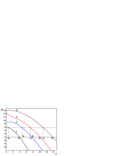
Figure 1: The dependencies of the chemical potential on temperature $\eta(\tau)$ at different values of the reduced density:
(1) $\tilde{n}_{\!L}=0.5$ ($\tau_{R}=0.68$, $\tau_{0}=3.96$); (2) $\tilde{n}_{\!L}=2.0$ ($\tau_{R}=4.76$, $\tau_{0}=7.68$); (3) $\tilde{n}_{\!L}=(2/\sqrt{\pi})\big{(}\rho_{2}^{2}-\rho_{1}^{2}\big{)}^{1\!/2}=3.37$ ($\tau_{R}=7.20$, $\tau_{0}=10.10$); (4) $\tilde{n}_{\!L}=6.0$ ($\tau_{R}=10.98$, $\tau_{0}=13.87$).

It is convenient to arrange the zeros of the Bessel function in ascending order with the help of a single new index $r\equiv(n,\nu)$, so that $\rho_{r+1}>\rho_{r}$, where $1\equiv(0,1)$ corresponds to the lowest value at which the Bessel function becomes zero $\rho_{1}=\rho_{01}$. The inequalities hold AS :

$$\begin{array}[]{ll}\displaystyle{\rho_{n1}<\rho_{n+1,1}<\rho_{n2}<\rho_{n+1,2}<\rho_{n3}<\rho_{n+1,3}<\ldots\,.}\end{array}$$ (34)

In Table I the ten first zeros of the Bessel function arranged in ascending order are given for reference. In this notation, the functions (6) are written in the form

$$\begin{array}[]{ll}\displaystyle{\Psi_{s}(\tau,\eta)\equiv\sum_{r=1}^{\infty}g_{r}\Phi_{s}\!\left[\tau^{-1}\big{(}\eta-\rho_{r}^{2}\big{)}\right],}\end{array}$$ (35)

where $g_{r}=1$ at $n=0$ and $g_{r}=2$ at $n\geq 1$.

Table 1: The ten first zeros of the Bessel function

$\rho_{1}=\rho_{0,1}$	$\rho_{2}=\rho_{1,1}$	$\rho_{3}=\rho_{2,1}$	$\rho_{4}=\rho_{0,2}$	$\rho_{5}=\rho_{3,1}$
2.40	3.83	5.14	5.52	6.38
$\rho_{6}=\rho_{1,2}$	$\rho_{7}=\rho_{4,1}$	$\rho_{8}=\rho_{2,2}$	$\rho_{9}=\rho_{0,3}$	$\rho_{10}=\rho_{5,1}$
7.02	7.59	8.42	8.65	8.77

In the high temperature region $\eta\leq\rho_{1}^{2}$ the functions (6) can be calculated by the formula

$$\begin{array}[]{ll}\displaystyle{\Psi_{s}(\tau,\eta)=\sum_{k=1}^{\infty}\!\frac{(-1)^{k+1}}{k^{s}}\sum_{r=1}^{\infty}g_{r}\,e^{k(\eta-\rho_{r}^{2})\!/\tau}}\end{array}$$ (36)

In the low temperature region $\eta>\rho_{1}^{2}$ there can be obtained asymptotic expansions for the functions (6), valid in the limit $\tau\rightarrow 0$. Let us represent the functions (6) in the form

$$\begin{array}[]{ll}\displaystyle{\Psi_{s}(\tau,\eta)=\vspace{2mm}}\\ \displaystyle{\hskip 2.84526pt=\sum_{r=1}^{r_{0}-1}\!g_{r}\Phi_{s}\!\left[\tau^{-1}\big{(}\eta-\rho_{r}^{2}\big{)}\right]+\sum_{r=r_{0}+2}^{\infty}\!g_{r}\Phi_{s}\!\left[\tau^{-1}\big{(}\eta-\rho_{r}^{2}\big{)}\right]+\vspace{2mm}}\\ \displaystyle{\hskip 2.84526pt+\,g_{r_{0}}\Phi_{s}\!\left[\tau^{-1}\big{(}\eta-\rho_{r_{0}}^{2}\big{)}\right]+g_{r_{0}+1}\Phi_{s}\!\left[\tau^{-1}\big{(}\eta-\rho_{r_{0}+1}^{2}\big{)}\right].}\end{array}$$ (37)

Here the index $r_{0}$, enumerating zeros, is defined by the condition: $\rho_{r_{0}}^{2}<\eta<\rho_{r_{0}+1}^{2}$. We singled out the third and the fourth terms, important at $\eta\geq\rho_{r_{0}}^{2}$ and $\eta\leq\rho_{r_{0}+1}^{2}$. At $\tau\ll 1$ the contribution of the second term is exponentially small, and for calculation of the first sum one should make use of the expansion being valid to within exponential corrections:

$$\begin{array}[]{l}\displaystyle{\Phi_{s}(t)=\frac{t^{s}}{s\Gamma(s)}\times\vspace{2mm}}\\ \displaystyle{\times\!\left\{1+2\sum_{k=0}^{\infty}\!\frac{s(s\!-\!\!1)\ldots(s\!-\!\!2k\!-\!\!1)(1\!-\!2^{\,-2k-\!1})\zeta(2k\!+\!2)}{t^{2k+2}}\!\right\}\!.}\end{array}$$ (38)

Finally, we obtain the asymptotic expansion valid in the limit $\tau\rightarrow 0$:

$$\begin{array}[]{ll}\displaystyle{\Psi_{s}(\tau,\eta)=\frac{1}{s\Gamma(s)\,\tau^{s}}\,Z_{s}^{(r_{0}-1)}(\eta)\,+\vspace{2mm}}\\ \displaystyle{+\frac{2}{\Gamma(s)}\!\sum_{k=0}^{\infty}\!b_{s}(2k\!+\!1\!)(1\!\!-\!2^{-2\!k-\!1}\!)\zeta(2k\!+\!2)\tau^{2\!k+2\!-\!s}Z_{s-2\!k-\!2}^{(r_{0}-1)}(\eta)+\vspace{2mm}}\\ \displaystyle{+\,g_{r_{0}}\Phi_{s}\!\left[\tau^{-1}\big{(}\eta-\rho_{r_{0}}^{2}\big{)}\right]+g_{r_{0}+1}\Phi_{s}\!\left[\tau^{-1}\big{(}\eta-\rho_{r_{0}+1}^{2}\big{)}\right],}\end{array}$$ (39)

where

$$\begin{array}[]{ll}\displaystyle{Z_{s}^{(r_{0})}(\eta)\equiv\sum_{r=1}^{r_{0}}g_{r}\big{(}\eta-\rho_{r}^{2}\big{)}^{s},}\end{array}$$ (40)

$b_{s}(m)=\prod_{l=1}^{m}(s-l)$ at $m\geq 1$, and $b_{s}(0)=1$. In particular, for the functions required in calculation of thermodynamic quantities, at $\tau\rightarrow 0$ it is sufficient to use the following approximations:

$$\begin{array}[]{ll}\displaystyle{\Psi_{1/2}(\tau,\eta)=\frac{2}{(\pi\tau)^{1/2}}\,Z_{1/2}^{(r_{0}-1)}(\eta)\,+\vspace{2mm}}\\ \displaystyle{\hskip 2.84526pt+\,g_{r_{0}}\Phi_{1/2}\!\left[\tau^{-1}\big{(}\eta-\rho_{r_{0}}^{2}\big{)}\right]+g_{r_{0}+1}\Phi_{1/2}\!\left[\tau^{-1}\big{(}\eta-\rho_{r_{0}+1}^{2}\big{)}\right],\vspace{3.8mm}}\\ \displaystyle{\Psi_{3/2}(\tau,\eta)=\frac{4}{3\sqrt{\pi}\tau^{3/2}}\left[Z_{3/2}^{(r_{0}-1)}(\eta)+\frac{\pi^{2}}{8}\,\tau^{2}Z_{-1/2}^{(r_{0}-1)}(\eta)\right]\!+\vspace{2mm}}\\ \displaystyle{\hskip 2.84526pt+\,g_{r_{0}}\Phi_{3/2}\!\left[\tau^{-1}\big{(}\eta-\rho_{r_{0}}^{2}\big{)}\right]+g_{r_{0}+1}\Phi_{3/2}\!\left[\tau^{-1}\big{(}\eta-\rho_{r_{0}+1}^{2}\big{)}\right].}\end{array}$$ (41)

In fact, at $\tau\leq 1$ these formulas approximate well the exact functions defined by the formula (6). Thus, at $\tau=0.1$ the error does not exceed 0.01%, and even at $\tau=1$ – 1%. The dependencies of these functions and their derivatives on the chemical potential are shown in Fig. 2. As seen (Fig. 2b), the function $\Psi_{3/2}(\tau,\eta)$ and its derivative monotonically increase with increasing the chemical potential. The function $\Psi_{1/2}(\tau,\eta)$ also monotonically increases but the behavior of its derivative has an oscillating character, besides the derivative has sharp maximums at the points corresponding to the zeros of the Bessel function (Fig. 2a). Note also that, since $\tilde{n}=\tilde{n}_{\!L}=\tau^{1/2}\Psi_{1/2}(\tau,\eta)$, the function $\Psi_{1/2}(\tau,\eta)$ describes the dependence of the reduced density, divided by $\tau^{1/2}$, on the chemical potential.

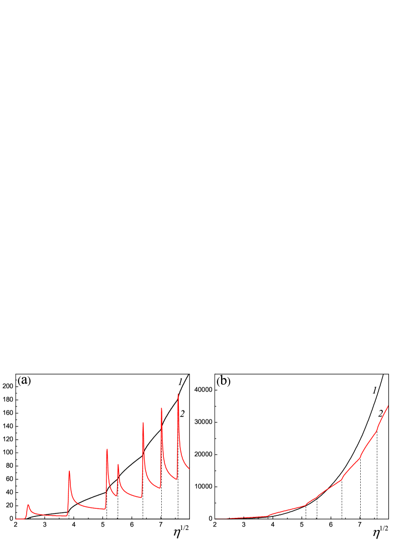
Figure 2: Graphs of the functions $\Psi_{1/2}(\tau,\eta)$, $\Psi_{3/2}(\tau,\eta)$ and their derivatives at $\tau=0.1$.
(a) The functions $\Psi_{1/2}(\tau,\eta)$ (1) and $\partial\Psi_{1/2}(\tau,\eta)\big{/}\partial\eta^{1/2}$ (2); (b) The functions $\Psi_{3/2}(\tau,\eta)$ (1) and $\partial\Psi_{3/2}(\tau,\eta)\big{/}\partial\eta^{1/2}$ (2).
The dashed lines correspond to the zeros of the Bessel function $\eta^{1/2}=\rho_{r}$.

VIII Thermodynamic quantities
at low temperatures

The most interesting range where the quantum effects may manifest themselves on the macroscopic level in the behavior of thermodynamic characteristics is the range of low temperatures. Let us consider the behavior of observable quantities at low temperatures such that $\tau\ll 1$ using the formulas (41). For the reduces densities of particles we have

$$\begin{array}[]{ll}\displaystyle{\tilde{n}=\tilde{n}_{\!L}=\tau^{1/2}\Psi_{1/2}(\tau,\eta)=\frac{2}{\sqrt{\pi}}\,Z_{1/2}^{(r_{0}-1)}(\eta)\,+\vspace{2mm}}\\ \displaystyle{+\tau^{1/2}\Big{\{}g_{r_{0}}\Phi_{1\!/2}\!\!\left[\tau^{-1}\!\big{(}\eta\!-\!\rho_{r_{0}}^{2}\!\big{)}\right]\!+g_{r_{0}+1}\Phi_{1\!/2}\!\!\left[\tau^{-1}\!\big{(}\eta\!-\!\rho_{r_{0}+1}^{2}\!\big{)}\right]\!\!\Big{\}}\!.}\end{array}$$ (42)

Here with a good accuracy the density can be considered independent of temperature and the formula $\tilde{n}=\tilde{n}_{\!L}\approx(2/\!\sqrt{\pi})Z_{1/2}^{(r_{0})}(\eta)$ can be used. The reduced entropy is determined by the formula

$$\begin{array}[]{ll}\displaystyle{\tilde{S}=\frac{2\pi^{3/2}}{9}\,Z_{-1/2}^{(r_{0}-1)}(\eta)\,\tau\,+\vspace{2mm}}\\ \displaystyle{+\,\tau^{1/2}\Big{\{}g_{r_{0}}\Phi_{3\!/2}\!\!\left[\tau^{-1}\!\big{(}\eta\!-\!\rho_{r_{0}}^{2}\!\big{)}\right]\!+g_{r_{0}+1}\Phi_{3\!/2}\!\!\left[\tau^{-1}\!\big{(}\eta\!-\!\rho_{r_{0}+1}^{2}\!\big{)}\right]\!-\vspace{2mm}}\\ \displaystyle{\hskip 34.1433pt-(2/3)\tau^{-1}\!\big{(}\eta\!-\!\rho_{r_{0}}^{2}\!\big{)}g_{r_{0}}\Phi_{1\!/2}\!\!\left[\tau^{-1}\!\big{(}\eta\!-\!\rho_{r_{0}}^{2}\!\big{)}\right]-\vspace{2mm}}\\ \displaystyle{\hskip 34.1433pt-(2/3)\tau^{-1}\!\big{(}\eta\!-\!\rho_{r_{0}+1}^{2}\!\big{)}g_{r_{0}+1}\Phi_{1\!/2}\!\!\left[\tau^{-1}\!\big{(}\eta\!-\!\rho_{r_{0}+1}^{2}\!\big{)}\right]\!\Big{\}}.}\end{array}$$ (43)

The terms which contain the functions $\Phi_{s}$ in (43) can be significant when $\eta\approx\rho_{r_{0}}^{2}$ or $\eta\approx\rho_{r_{0}+1}^{2}$. It should be noted that in the quasi-one-dimensional case, the same as in the volume and the quasi-two-dimensional PS cases, nearly everywhere except the specific points there remains the linear dependence of the entropy on temperature (see Fig. 3), and the following formula can be used

$$\begin{array}[]{ll}\displaystyle{\tilde{S}\approx\frac{2\pi^{3/2}}{9}\,Z_{-1/2}^{(r_{0})}(\eta)\,\tau.}\end{array}$$ (44)

The slope of the lines (44) and the width of the range where this formula is valid depend on the closeness of the chemical potential value to the square of the Bessel function zero. As the chemical potential approaches the square of the Bessel function zero from the side of greater values $\eta\rightarrow\rho_{r_{0}}^{2}+0$ the slope angle of a line increases (curve 2 in Fig. 3) and at the very point $\eta=\rho_{r_{0}}^{2}$, as it follows from the formula (43), $\tilde{S}\sim\sqrt{\tau}$ (curve 1 in Fig. 3). As the chemical potential approaches the square of the Bessel function zero from the side of smaller values $\eta\rightarrow\rho_{r_{0}}^{2}-0$ the slope angle of a line tends to a finite value (curve 3 in Fig. 3), at that, however, the temperature range where the linear dependence is realized proves to be quite narrow.

The dependence of the reduced entropy on the dimensionless chemical potential is presented in Fig. 4. As we see, the entropy has sharp maximums at the points where the chemical potential equals the square of the Bessel function zero. At calculation by means of the approximate formula (44) while approaching the point $\eta=\rho_{r_{0}}^{2}$ from the right there is the root singularity $\tilde{S}\sim\big{(}\eta-\rho_{r_{0}}^{2}\big{)}^{\!-1\!/2}$, and while approaching this point from the left the entropy takes a finite value. The calculation by the more accurate formula (43) eliminates the singularity and allows to obtain the entropy value at the maximum $\tilde{S}_{\rm{max}}$, which with a good accuracy is determined by the formula

$$\begin{array}[]{ll}\displaystyle{\tilde{S}_{\rm{max}}\approx\tilde{S}(\tau,\eta_{r_{0}})\approx\vspace{2mm}}\\ \displaystyle{\hskip 8.53581pt\approx\!\frac{2\pi^{3/2}}{9}\,Z_{-1/2}^{(r_{0}-1)}(\eta_{r_{0}})\,\tau+g_{r_{0}}\!\big{(}1\!-\!2^{-1/2}\big{)}\zeta(3/2)\sqrt{\tau},}\end{array}$$ (45)

where $\zeta(3/2)\approx 2.612$ is the Riemann zeta function. Pay attention that the values of maximums for the nondegenerate levels with $n=0$  turn out to be less than the appropriate values for the neighboring levels with the two-fold degeneracy at $n\neq 0$ (see Fig. 4).

In the quasi-one-dimensional case under study the dependence of the entropy on the chemical potential is qualitatively different from the quasi-two-dimensional case PS , i.e. the entropy has a sharp maximum rather than undergoes a jump at the beginning of the filling of a new discrete level. One more difference of the given system from the quasi-two-dimensional case is the irregularity of the values of chemical potential, specified by the Bessel function zeros, at which the entropy has peculiarities PS .

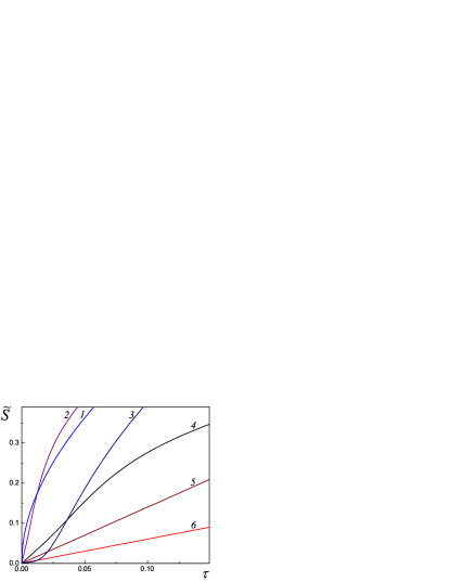
Figure 3: The dependence of the reduced entropy $\tilde{S}(\tau,\eta)$ on the temperature $\tau$ at a fixed value of the chemical potential:
(1) $\eta=\rho_{2}^{2}=\rho_{1,1}^{2}=14.68$ ($\tilde{n}_{\!L}=3.37$); (2) $\eta=14.72$ ($\tilde{n}_{\!L}=3.81$); (3) $\eta=14.60$ ($\tilde{n}_{\!L}=3.35$); (4) $\eta=5.98$ ($\tilde{n}_{\!L}=0.5$);
(5) $\eta=20.0$ ($\tilde{n}_{\!L}=9.46$); (6) $\eta=10.0$ ($\tilde{n}_{\!L}=2.32$).
The density $\tilde{n}_{\!L}$ is given at $\tau=0$.

In the main approximation all introduced above heat capacities (23) – (26), as it had to be expected, prove to be identical and coinciding with the entropy. Thus, in the quasi-one-dimensional case, the same as in the quasi-two-dimensional PS and the volume cases, all heat capacities prove to be proportional to temperature:

$$\begin{array}[]{ll}\displaystyle{\tilde{C}=\frac{2\pi^{3/2}}{9}\,Z_{-1/2}^{(r_{0})}(\eta)\,\tau.}\end{array}$$ (46)

Only at the specific points, at $\eta\rightarrow\rho_{r_{0}}^{2}+0$, the same as in the entropy case, there appears the dependence $\tilde{C}\sim\sqrt{\tau}$. The temperature dependence of heat capacities and their dependence on the chemical potential are similar to the dependencies for the entropy shown in Figs.  3 and 4.

It is interesting to consider the transition from the formulas (44), (46) to the volume case, when the radius of the tube becomes large as compared with the de Broglie wavelength. It can be done, if one takes into account that in order to make the transition from the dispersion law of particles in the tube (2) to the dispersion law of free particles it is necessary to make the substitution

$$\begin{array}[]{l}\displaystyle{\rho_{n\nu}^{2}\frac{\hbar^{2}}{2mR^{2}}\,\rightarrow\,\frac{\hbar^{2}(k_{x}^{2}+k_{y}^{2})}{2m}.}\end{array}$$ (47)

The same rule of transition to the continuous spectrum can be obtained by means of the asymptotic expression for the Bessel functions.

Performing formally the same substitution at calculation of the functions (41) and replacing the summation over the Bessel function zeros by the integration over the wave vector in the $(x,y)$ plane, we obtain

$$\begin{array}[]{ll}\displaystyle{Z_{1/2}(\eta)=\frac{\sqrt{2}(m\mu)^{3/2}R^{3}}{3\hbar^{3}},\quad Z_{-1/2}(\eta)=\frac{(m\mu)^{1/2}R}{\sqrt{2}\hbar}.}\end{array}$$ (48)

Finally, we come to the known volume expressions for the particle number density $n=(2m\mu)^{3/2}\!\big{/}3\pi^{2}\hbar^{3}$ and also the entropy and the heat capacity $S=C=\big{(}m^{3/2}(2\mu)^{1/2}\!\big{/}3\hbar^{3}\big{)}VT$.

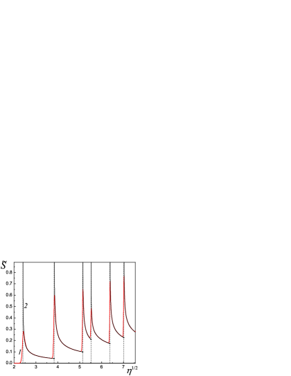
Figure 4: The dependence of the reduced entropy $\tilde{S}(\tau,\eta)$ on the chemical potential. The curve ${\it 1}$ is plotted by means of the formula (43), and the curve ${\it 2}$ – by the formula (44) at $\tau=0.1$. The dashed lines correspond to the zeros of the Bessel function $\eta^{1/2}=\rho_{r}$.

Let us give the results of calculation of the reduced pressures at zero temperature. In this case the pressures are determined by the formulas:

$$\begin{array}[]{ll}\displaystyle{\tilde{p}_{\parallel}=\frac{4}{3\sqrt{\pi}}\,Z_{3/2}^{(r_{0})}(\eta),}\end{array}$$ (49)

$$\begin{array}[]{ll}\displaystyle{\tilde{p}_{R}=\frac{2}{\sqrt{\pi}}\Big{[}\eta Z_{1/2}^{(r_{0})}(\eta)-Z_{3/2}^{(r_{0})}(\eta)\Big{]}.}\end{array}$$ (50)

The dependencies of the pressures (49) and (50) on the chemical potential are shown in Fig. 5. As seen, the parallel pressure smoothly increases with increasing the chemical potential, and the radial pressure undergoes breaks (discontinuities in the derivative) at the points where the filling of a new discrete level begins. In the volume case, considering the formula $Z_{3/2}(\eta)=2^{3/2}(m\mu)^{5/2}R^{5}\!\big{/}5\hbar^{5}$, the both formulas (49) and (50) lead to the known expression for the pressure of the Fermi gas at zero temperature: $p=\big{(}2^{5/2}\!\big{/}15\pi^{2}\big{)}\,m^{3/2}\mu^{5/2}\!\big{/}\hbar^{3}.$

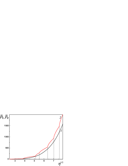
Figure 5: The dependencies of the reduced pressures on the chemical potential at zero temperature: (1) $\tilde{p}_{\parallel}(\eta)$; (2) $\tilde{p}_{R}(\eta)$. Dashed lines correspond to the zeros of the Bessel function.

Let us proceed to consideration of the compressibilities. The reduced compressibilities at zero temperature are determined be the formulas:

$$\begin{array}[]{ll}\displaystyle{\tilde{\gamma}_{\parallel}=\frac{\sqrt{\pi}}{4}\frac{Z_{-1/2}^{(r_{0})}(\eta)}{\big{[}Z_{1/2}^{(r_{0})}(\eta)\big{]}^{2}},\vspace{1mm}}\\ \displaystyle{\tilde{\gamma}_{R}=\!\frac{\sqrt{\pi}\,Z_{-1\!/2}^{(r_{0})}(\eta)}{4\eta Z_{1\!/2}^{(r_{0})}\!(\eta)Z_{-1\!/2}^{(r_{0})}\!(\eta)\!-\!5Z_{3\!/2}^{(r_{0})}\!(\eta)Z_{-1\!/2}^{(r_{0})}\!(\eta)\!+\!\!\big{[}Z_{1\!/2}^{(r_{0})}\!(\eta)\big{]}^{2}}.}\end{array}$$ (51)

The dependencies of the compressibilities (51) on the chemical potential are shown in Fig. 6. While approaching the point where the filling of a new level begins from the side of smaller values of the chemical potential the parallel compressibility has a finite value, and while approaching the specific point from the side of greater values of the chemical potential – it tends to infinity. The radial compressibility has finite maximums in the specific points, such that the magnitude of peaks rapidly decreases with increasing the chemical potential. In the volume limit the both compressibilities coincide, being given by the formula

$$\begin{array}[]{ll}\displaystyle{\gamma_{\parallel}=\gamma_{R}=\frac{9\pi^{2}}{4\sqrt{2}}\frac{\hbar^{3}}{m^{3/2}\mu^{5/2}}.}\end{array}$$ (52)

Since the square of speed of sound $u^{2}=m^{-1}\big{(}\partial p/\partial n\big{)}$ and the compressibility are connected by the relation $u^{2}=1\big{/}mn\gamma$, then from (52) it follows the known formula for the speed of sound in the Fermi gas at zero temperature: $u^{2}=(2/3)\,\mu/m$.

Figure 6: The dependencies of the compressibilities on the chemical potential at zero temperature: (1) $\tilde{\gamma}_{\parallel}(\eta)$; (2) $\tilde{\gamma}_{R}(\eta)$. Dashed lines correspond to the zeros of the Bessel function.

The peculiarities considered above in the behavior of the entropy, heat capacities, pressures and compressibilities of the quasi-one-dimensional system and their difference from those of the quasi-two-dimensional system are connected with the form of the density of states $\nu(\varepsilon)$, which is shown in Fig. 7 for the quasi-two-dimensional quantum well and the quasi-one-dimensional tube. In the case of the quantum well the density of states is constant and changes by a jump at the beginning of the filling of a new level (Fig. 7a). In the quasi-one-dimensional case the density of states tends to infinity $\nu(\varepsilon)\sim\big{(}\varepsilon-\rho_{r}^{2}\varepsilon_{R}\big{)}^{\!-1/2}$ at $\varepsilon\rightarrow\rho_{r}^{2}\varepsilon_{R}+0$ (Fig. 7b). Such a dependence of the density of states on the energy is similar to that which takes place for electrons in magnetic field. The difference consists in that in magnetic field the peculiarities are distributed regularly with the intervals multiple of odd numbers of half the cyclotron frequency. In the considered case the distribution of the peculiarities is irregular and is determined by the zeros of the Bessel function.

Figure 7: The density of states for the quasi-two-dimensional quantum well and the nanotube:
(a) $\bar{\nu}_{\rm{2D}}(\tilde{\varepsilon})=\nu_{\rm{2D}}(\tilde{\varepsilon})\left(\frac{mA}{\pi\hbar^{2}}\right)^{\!-1}\!=\sum_{n=1}^{\infty}\theta(\tilde{\varepsilon}\!-\!n^{2}),\,\tilde{\varepsilon}=\varepsilon\big{/}\varepsilon_{L},\,\varepsilon_{L}\!\equiv\!\frac{\pi^{2}\hbar^{2}}{2mL_{0}^{2}}$, $A$ is the area, $L_{0}$ is the distance between planes PS ;
(b) $\bar{\nu}_{\rm{1D}}(\tilde{\varepsilon})=\nu_{\rm{1D}}(\tilde{\varepsilon})\left(\frac{2mLR}{\pi\hbar^{2}}\right)^{\!-1}\!=Z_{-1/2}^{(r_{0})}(\tilde{\varepsilon})$  at  $\rho_{r_{0}}^{2}<\tilde{\varepsilon}\leq\rho_{r_{0}+1}^{2}$, $\tilde{\varepsilon}=\varepsilon\big{/}\varepsilon_{R}$. The dashed lines correspond to $\tilde{\varepsilon}=\rho_{r}^{2}$.

IX Dependencies of thermodynamic quantities on the tube radius

If thermodynamic quantities are taken in the reduced form (19), and the dimensionless chemical potential $\eta$ and the dimensionless temperature $\tau$ are used as independent variables, then as it was shown the geometrical dimensions fall out of the thermodynamic relations, in particular the radius of the tube $R$ falls out. Meanwhile, exactly the dependencies of the observable quantities on the tube radius are of interest in experiment. To obtain such dependencies, the relations derived above should be presented in the dimensional form. At that, the form of dependence of the thermodynamic quantities on the radius will essentially depend on what quantity is being fixed when studying such dependence: the total density $n$ or the linear density $n_{\!L}$. Let us show it on the example of dependence of the chemical potential on the tube radius. In the dimensional form the formulas for the densities can be presented as follows

$$\begin{array}[]{ll}\displaystyle{\pi^{3/2}R^{3}n=\pi^{1/2}R\,n_{\!L}=\frac{2}{\sqrt{\pi}}\,Z_{1/2}^{(r_{0})}(\eta),}\end{array}$$ (53)

and, according the definition, the chemical potential is expressed through the parameter $\eta$ by the formula

$$\begin{array}[]{ll}\displaystyle{\mu=\frac{\hbar^{2}}{2mR^{2}}\,\eta.}\end{array}$$ (54)

The formulas (53) and (54) define parametrically the dependence of the chemical potential on the radius in the domain of variation of the parameter $\rho_{r_{0}}^{2}<\eta<\rho_{r_{0}+1}^{2}$. As we see, the dependence of $R$ on the parameter $\eta$ will be different depending on what is fixed – the volume or the linear density.

At the fixed linear density $n_{\!L}=\rm{const}$ in the domain $\rho_{r_{0}}^{2}<\eta<\rho_{r_{0}+1}^{2}$ the dependence of the chemical potential on the radius is parametrically defined by the equations

$$\begin{array}[]{ll}\displaystyle{\bar{\mu}=\frac{\eta}{\big{[}Z_{1/2}^{(r_{0})}(\eta)\big{]}^{2}},\quad\bar{R}=Z_{1/2}^{(r_{0})}(\eta),}\end{array}$$ (55)

where

$$\begin{array}[]{ll}\displaystyle{\bar{R}=\frac{\pi n_{\!L}}{2}R,\quad\bar{\mu}=\frac{2m}{\hbar^{2}}\Big{(}\frac{2}{\pi n_{\!L}}\Big{)}^{\!2}\mu.}\end{array}$$ (56)

At the fixed total density $n=\rm{const}$ the similar dependence is defined by the equations

$$\begin{array}[]{ll}\displaystyle{\bar{\mu}=\frac{\eta}{\big{[}Z_{1/2}^{(r_{0})}(\eta)\big{]}^{2/3}},\quad\bar{R}=\big{[}Z_{1/2}^{(r_{0})}(\eta)\big{]}^{1/3},}\end{array}$$ (57)

where

$$\begin{array}[]{ll}\displaystyle{\bar{R}=\Big{(}\frac{\pi^{2}n}{2}\Big{)}^{\!1/3}R,\quad\bar{\mu}=\frac{2m}{\hbar^{2}}\Big{(}\frac{2}{\pi^{2}n}\Big{)}^{\!2/3}\mu.}\end{array}$$ (58)

The dependencies of the chemical potential on the tube radius are shown for both cases in Fig. 8. As seen, at the fixed linear density the chemical potential monotonically decreases with increasing the radius (curve 1 in Fig. 8). The oscillation dependence on the radius is realized at the fixed total density (curve 2 in Fig. 8). The amplitude of oscillations rapidly decreases with increasing the radius, at that the chemical potential quite slowly approaching its volume value $\displaystyle{\bar{\mu}_{\rm{3D}}=\lim_{\bar{R}\rightarrow\infty}\bar{\mu}=6^{2/3}}$.

Let us also give the dependencies on the radius of such a directly measurable quantity as the pressure. At the fixed linear density $n_{\!L}=\rm{const}$ in the domain $\rho_{r_{0}}^{2}<\eta<\rho_{r_{0}+1}^{2}$ the dependencies of the radial and the parallel pressures on the parameter $\eta$ are defined by the formulas:

$$\begin{array}[]{ll}\displaystyle{\bar{p}_{R}=\frac{\eta Z_{1/2}^{(r_{0})}(\eta)-Z_{3/2}^{(r_{0})}(\eta)}{\big{[}Z_{1/2}^{(r_{0})}(\eta)\big{]}^{5}},\quad\bar{p}_{\parallel}=\frac{2}{3}\frac{Z_{3/2}^{(r_{0})}(\eta)}{\big{[}Z_{1/2}^{(r_{0})}(\eta)\big{]}^{5}},}\end{array}$$ (59)

where

$$\begin{array}[]{ll}\displaystyle{\bar{p}_{R,\parallel}=\pi^{2}\frac{m}{\hbar^{2}}\Big{(}\frac{2}{\pi n_{\!L}}\Big{)}^{\!5}p_{R,\parallel}}\end{array}$$ (60)

and the dependence of the radius on $\eta$ is given by the formulas (55),(56). At the fixed total density $n=\rm{const}$ the similar dependencies are defined by the equations

$$\begin{array}[]{ll}\displaystyle{\bar{p}_{R}=\!\frac{\eta Z_{1/2}^{(r_{0})}(\eta)-Z_{3/2}^{(r_{0})}(\eta)}{\big{[}Z_{1/2}^{(r_{0})}(\eta)\big{]}^{5/3}},\,\,\,\bar{p}_{\parallel}=\!\frac{2}{3}\frac{Z_{3/2}^{(r_{0})}(\eta)}{\big{[}Z_{1/2}^{(r_{0})}(\eta)\big{]}^{5/3}},}\end{array}$$ (61)

where

$$\begin{array}[]{ll}\displaystyle{\bar{p}_{R,\parallel}=\pi^{2}\frac{m}{\hbar^{2}}\Big{(}\frac{2}{\pi^{2}n}\Big{)}^{5/3}p_{R,\parallel}\,,}\end{array}$$ (62)

and the dependence of the radius on $\eta$ is given by the formulas (57),(58). The dependencies of the pressures on the tube radius are shown for both cases in Fig. 9.

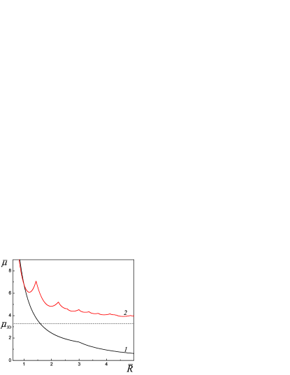
Figure 8: The dependencies of the chemical potential on the tube radius: ​(1) at the fixed linear density $n_{\!L}$ ($\bar{\mu},\bar{R}$ are defined by formulas (56)); ​(2) at the fixed volume density $n$ ($\bar{\mu},\bar{R}$ are defined by formulas (58)). The dashed line shows the chemical potential $\displaystyle{\bar{\mu}_{\rm{3D}}\!=\!\lim_{\bar{R}\rightarrow\infty}\bar{\mu}=6^{2/3}}$ of volume system of density $n$.

Here also, the oscillations exist only under condition of the fixed total density, so that qualitatively the situation in this quasi-one-dimensional case is similar to that which takes place in the quasi-two-dimensional quantum well PS . At the fixed linear density $n_{\!L}$ with increasing the radius the total density $n$ approaches zero, so that the both pressures approach zero as well. In the opposite case $R\rightarrow 0$ the total density increases unlimitedly and therefore the pressures also tend to infinity (curves 1, 2 in Fig. 9). At the fixed total density $n$ with increasing the radius the both pressures approach, oscillating, their volume value $\displaystyle{\bar{p}_{\rm{3D}}=\!\lim_{\bar{R}\rightarrow\infty}\bar{p}_{R,\parallel}=(2/5)6^{2/3}}$. In the limit $R\rightarrow 0$  it should be $L\rightarrow\infty$, and so the linear density $n_{\!L}\rightarrow 0$. Hence the parallel pressure also approaches zero $p_{\parallel}\rightarrow 0$. The radial pressure with decreasing the tube radius tends to infinity $p_{R}\rightarrow\infty$ due to the zero-point oscillations in the radial direction (curves 3, 4 in Fig. 9).

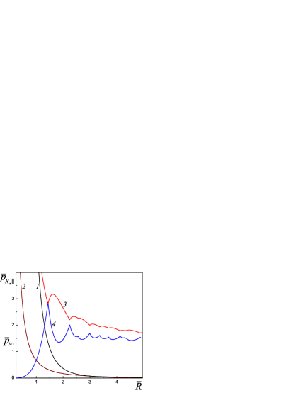
Figure 9: The dependencies of the pressures on the tube radius: ​(1) $\bar{p}_{R}(\bar{R})$ and (2) $\bar{p}_{\parallel}(\bar{R})$ at the fixed linear density $n_{\!L}$; (3) $\bar{p}_{R}(\bar{R})$ and (4) $\bar{p}_{\parallel}(\bar{R})$ at the fixed volume density $n$. The dashed line shows the pressure $\displaystyle{\bar{p}_{\rm{3D}}=\!\lim_{\bar{R}\rightarrow\infty}\bar{p}_{R,\parallel}=(2/5)6^{2/3}}$ of volume system of density $n$.

X Conclusion

The exact formulas for calculation of the thermodynamic functions of the ideal Fermi gas that fills the tube of an arbitrary radius at arbitrary temperature have been derived in the work. It is shown that all thermodynamic quantities, written in the dimensionless reduced form not containing geometric dimensions, can be expressed through some standard functions (6) of the dimensionless temperature and chemical potential and their derivatives. The thermodynamic potential, energy, density, entropy, equations of state, heat capacities and compressibilities of the Fermi gas at arbitrary temperatures in the considered quasi-one-dimensional case are calculated through the introduced standard functions. It is shown that owing to the anisotropy of the system the Fermi gas has two equations of state since the pressures along the tube and in the direction of its radius are different. Due to the same reason the system is characterized by more number of heat capacities than in the volume case.

At low temperatures the entropy and all heat capacities are linear in temperature everywhere except the specific points where the chemical potential coincides with the square of the Bessel function zero and the filling of a new discrete level begins. At these specific points the root dependence of the entropy and heat capacities on temperature appears. The dependencies of the entropy and heat capacities on the chemical potential have sharp maximums at the specific points. This differs the quasi-one-dimensional case from the the quasi-two-dimensional where the heat capacities and entropy undergo jumps at the beginning of the filling of a new discrete level. The dependencies of the pressures and compressibilities on the chemical potential at zero temperature are calculated. It is shown that the character of dependence of thermodynamic quantities on the tube radius essentially depends on whether this dependence is considered at the fixed linear or the fixed total density. At the fixed linear density the thermodynamic quantities vary monotonically with the radius, and at the fixed total density they undergo oscillations.​ We believe that the results of this work and work PS devoted to the quasi-two-dimensional system can serve as a basis for further consistent study of low-dimensional systems of interacting Fermi particles.

References

- (1) T. Ando, A.B. Fowler, and F. Stern, Electronic properties of two-dimensional systems, Rev. Mod. Phys. 54, 437 (1982). doi: 10.1103/RevModPhys.54.437
- (2) Y.F. Komnik, Physics of metal films (in Russian), Atomizdat, Moscow, 264 p. (1979).
- (3) V.P. Dragunov, I.G. Neizvestnyj, V.A. Gridchin, Fundamentals of nanoelectronics (in Russian), Fizmatkniga, Moscow, 496 p. (2006).
- (4) I.D. Vagner, Thermodynamics of two-dimensional electrons on Landau levels, HIT J. of Science and Engineering A 3, 102 – 152 (2006).
- (5) D.M. Freik, L.T. Kharun, A.M. Dobrovolska, Quantum-size effects in condensed systems. Scientific and historical aspects, Phys. and Chem. of Solid State 12, 9 – 26 (2011).
- (6) V.R. Shaginyan, K.G. Popov, Strongly correlated Fermi-systems: theory versus experiment, Nanostructures. Mathematical physics and modeling 3, 5 – 92 (2010).
- (7) L.D. Landau, E.M. Lifshitz, Statistical physics, Vol. 5, Butterworth-Heinemann, Oxford, 544 p. (1980).
- (8) Yu.M. Poluektov, A.A. Soroka, Thermodynamics of the Fermi gas in a quantum well, East Eur. J. Phys. 3 (4), 4 – 21 (2016); arXiv:1608.07205 [cond-mat.stat-mech].
- (9) S. Tomonaga, Remarks on Bloch’s method of sound waves applied to many-fermion problems, Progr. Theor. Phys. 5, 544 – 569 (1950). doi: 10.1143/ptp/5.4.544
- (10) J.M. Luttinger, An exactly soluble model of a many-fermion system, J. Math. Phys. 4, 1154 – 1162 (1963). doi: 10.1063/1.1704046
- (11) V.V. Deshpande, M. Bockrath, L.I. Glazman, A. Yacoby, Electron liquids and solids in one dimension, Nature 464 (11), 209 – 216 (2010). doi: 10.1038/nature08918
- (12) L.D. Landau, The theory of a Fermi liquid, Sov. Phys. JETP 3, 920 – 925 (1957).
- (13) D. Pines, P. Nozières, The theory of quantum liquids, Vol. I, Benjamin, New York, 149 p. (1966).
- (14) M. Abramowitz, I. Stegun (Editors), Handbook of mathematical functions, Nauka, Moscow, 832 p. (1979).