Measurement and control of a Coulomb-blockaded parafermion box

Abstract

Parafermionic zero modes are fractional topologically protected quasiparticles expected to arise in various platforms. We show that Coulomb charging effects define a parafermion box with unique access options via fractional edge states and/or quantum antidots. Basic protocols for the detection, manipulation, and control of parafermionic quantum states are formulated. With those tools, one may directly observe the dimension of the zero-mode Hilbert space, prove the degeneracy of this space, and perform on-demand digital operations satisfying a parafermionic algebra.

Introduction. Majorana zero modes are canonical examples for topologically protected quasiparticles with non-Abelian braiding statistics Nayak2008 ; Alicea2012 ; Leijnse2012 ; Beenakker2013 . In the presence of Coulomb charging effects, intriguing features related to their nonlocality have been pointed out Fu2010 ; Beri2012 ; Altland2013 ; Beri2013 ; Landau2016 ; Aasen2016 ; Vijay2016 ; Plugge2017 ; Karzig2016 and probed experimentally Albrecht2016 ; Albrecht2017 . The drive for reaching universal quantum computation platforms and the quest to fully understand topological excitations have turned attention to exotic emergent quasiparticles such as parafermions (PFs) with $\mathbb{Z}_{n>2}$ symmetry. For PF zero modes, a plethora of interesting phenomena has been suggested in various platforms Lindner2012 ; Cheng2012 ; Clarke2013 ; Burrello2013 ; Vaezi2013 ; Zhang2014 ; Mong2014 ; Clarke2014 ; Barkeshli2014a ; Barkeshli2014b ; Cheng2015 ; Alicea2015a ; Kim2017 ; for a review, see Ref. Alicea2016 . For one-dimensional (1D) interacting fermions, Ref. Fidkowski2011 suggests that Majorana states exhaust all possibilities in the generic (disordered) case. However, Refs. Klinovaja2014 ; Klinovaja2014b show that PFs can exist in models of 1D nanowires. Moreover, for edge states of a fractionalized two-dimensional system, such as the fractional quantum Hall (FQH) liquid, domain walls between regions proximitized by a superconductor (SC) foot:SC+magnetic_field and a ferromagnet (FM) host stable PFs. Platforms for PFs include proximitized fractional topological insulators Lindner2012 , bilayer FQH systems Barkeshli2014b , and proximitized FQH liquids at a filling factor of $\nu=2/3$ Mong2014 or $\nu=1/(2k+1)$ with an integer $k$ Lindner2012 ; Clarke2013 . Such setups may ultimately provide a toolbox for generating Fibonacci anyons Mong2014 ; Alicea2015a , which, in turn, facilitate fault-tolerant universal quantum computation.

In the present Rapid Communication we leap beyond the interesting platforms alluded to above. We point out that PF devices dominated by Coulomb charging effects provide direct detection and manipulation tools targeting the fundamental physics of PFs. Specifically, we show below how one can: (i) measure the dimension of the Hilbert space associated with PF zero modes, (ii) render this space degenerate in a controlled manner, and (iii) explicitly demonstrate the exotic algebra of PF operators. By combining systems made of fractionalized bulk matter with mesoscopic sensing concepts, all superimposed on Coulomb charging effects, the PF box (cf. Fig. 1) facilitates full access to the beautiful physics of PF zero modes. Recent Majorana experiments Albrecht2016 ; Albrecht2017 also attest to the promise of such an approach. Probing these core facets of PF Hilbert space is realized employing fractional edge states [for current measurements] and quantum antidots (QADs) [for elastic cotunneling of quasiparticles through the box]. Such major facets are hard (if not impossible) to access otherwise, e.g., using multiple Josephson periodicities Lindner2012 ; Cheng2012 ; Clarke2013 ; Vaezi2013 ; Zhang2014 ; Cheng2015 ; foot1 , zero-bias anomalies Clarke2014 , split conductance peaks due to finite-size effects Barkeshli2014a , or quantized conductance measurements Kim2017 ; foot1 . Apart from being interesting in its own right, e.g., in the context of topological Kondo effects Beri2012 , it stands to reason that the experimental implementation of the PF box would pave the way for realizing PF-based quantum information devices foot_control-by-meas .

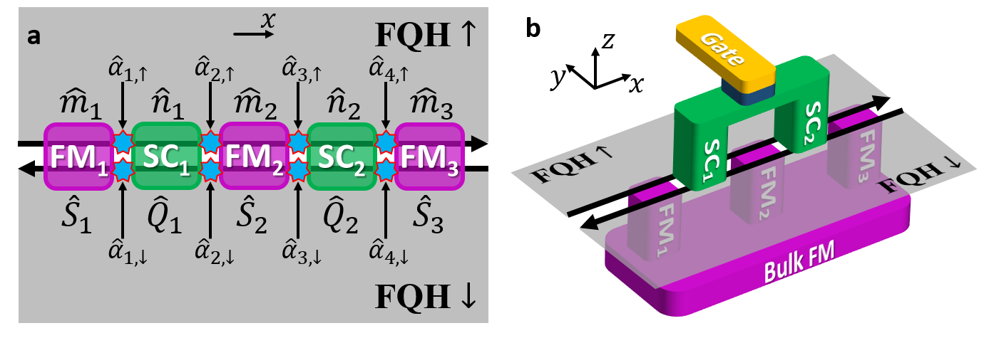
Figure 1: Layout of the PF box. (a) Two opposite-spin FQH edges (the thick black arrows) are gapped out in distinct ways via proximitizing FM and SC segments in different regions. PF operators $\hat{\alpha}_{j,s}$ (the blue stars) are localized at domain walls. (b) SC segments are electrically connected to ensure phase coherence across different SC domains. Similarly, FM segments belong to one bulk FM. The gate (golden), separated (insulating blue layer) from the SC bridge, can be used to change the offset charge $q_{\mathrm{g}}$ while disturbing the rest of the system only minimally. A back gate that can tune the chemical potential of the FQH puddles is implied.

PF box model. For concreteness, we study an array of PF zero modes implemented via two $\nu=1/(2k+1)$ FQH puddles of opposite spin Lindner2012 ; Clarke2013 ; foot_Heiblum , cf. Fig. 1. Our proposal is adaptable to other platforms (see the Supplemental Matterial SupplMat ); for $\nu=1$ it is reduced to a Majorana setup Plugge2017 . The puddle edges are described by bosonic fields $\hat{\phi}_{s=\uparrow/\downarrow=\pm 1}(x)$ with commutator Clarke2013

$$[\hat{\phi}_{s}(x),\hat{\phi}_{s}(x^{\prime})]=is\pi\mathrm{sgn}(x-x^{\prime}),\quad[\hat{\phi}_{\uparrow}(x),\hat{\phi}_{\downarrow}(x^{\prime})]=i\pi.$$ (1)

The resulting fractional helical edge state can be gapped by proximity coupling to SC or FM segments, see Fig. 1(a), with the Hamiltonian $H_{0}=H_{\mathrm{edge}}+H_{\mathrm{SC}}+H_{\mathrm{FM}}+H_{\mathrm{C}}$, where $H_{\mathrm{edge}}=(v/4\pi)\sum_{s}\int_{-\infty}^{\infty}dx(\partial_{x}\hat{\phi}_{s})^{2}$ with edge velocity $v$. Furthermore,

$$H_{\mathrm{SC}} = -\Delta\sum_{j=1}^{N}\int_{\mathrm{SC}_{j}}dx\cos\left(\frac{\hat{\phi}_{\uparrow}(x)+\hat{\phi}_{\downarrow}(x)}{\sqrt{\nu}}+\hat{\varphi}\right),$$ (2)

$$H_{\mathrm{FM}} = -t\sum_{j=1}^{N+1}\int_{\mathrm{FM}_{j}}dx\cos\left(\frac{\hat{\phi}_{\uparrow}(x)-\hat{\phi}_{\downarrow}(x)}{\sqrt{\nu}}\right).$$ (3)

$H_{\mathrm{SC}}$ describes the SC pairing induced in the edges by the proximitizing SCs, where $\hat{\varphi}$ is the SC phase operator and $\Delta$ is the absolute value of the induced pairing amplitude. $H_{\mathrm{FM}}$ describes electron hopping between the edges accompanied by a spin flip, which is enabled by the presence of the FM. The hopping amplitude $t$ is proportional to the FM in-plane magnetization caused by, e.g., geometrical effects. All the proximitizing SCs (FMs) are implied to be parts of one common SC (FM), see Fig. 1(b). For a floating (not grounded) SC, the charging term is $H_{\mathrm{C}}=(\hat{Q}_{0}-q_{\mathrm{g}})^{2}/(2C_{\mathrm{SC}})$, with the charge $\hat{Q}_{0}$ satisfying $[\hat{\varphi},\hat{Q}_{0}]=2i$. The offset charge $q_{\mathrm{g}}$ is controlled by a gate [Fig. 1(b)]. Finally, the charge and spin of an edge segment are given by

$$\left.\begin{array}[]{c}\hat{Q}_{AB}\\ \hat{S}_{AB}\end{array}\right\}=\int_{A}^{B}dx(\hat{\rho}_{\uparrow}\pm\hat{\rho}_{\downarrow}),\quad\hat{\rho}_{s}(x)=\frac{s\sqrt{\nu}}{2\pi}\partial_{x}\hat{\phi}_{s}.$$ (4)

A parafermion $N$-box is then defined by $N+1$ FM and $N$ SC domains excluding the outer edges. For instance, Fig. 1 shows a two-box.

Low-energy theory. The quasiparticle excitations in the SC and FM domains have gaps $(4\pi v\Delta/\nu)^{1/2}$ and $(4\pi vt/\nu)^{1/2}$, respectively Lindner2012 . At energies below these scales foot:qp_poisoning , the problem can be simplified using the method of Ref. Ganeshan2016 since the large cosines in Eqs. (2) and (3) imply that each FM (SC) domain is then effectively described by an integer-valued operator $\hat{m}_{j}$ ($\hat{n}_{j}$), see Refs. Lindner2012 ; Clarke2013 and Fig. 1(a),

$$\left.\frac{\hat{\phi}_{\uparrow}(x)\mp\hat{\phi}_{\downarrow}(x)}{2\pi\sqrt{\nu}}\right|_{x\in\mathrm{FM}_{j}/\mathrm{SC}_{j}}=\left\{\begin{array}[]{c}\hat{m}_{j},\\ \hat{n}_{j}-\hat{\varphi}/(2\pi).\end{array}\right.$$ (5)

The only nontrivial commutation relation is $[\hat{m}_{j},\hat{n}_{l}]=i/(\pi\nu)$ for $j>l$, whereas $[\hat{m}_{j},\hat{n}_{l}]=0$ for $j\leq l$. Using Eq. (4), the charge $\hat{Q}_{j}$ (spin $\hat{S}_{j}$) of the edge segment corresponding to $\mathrm{SC}_{j}$ ($\mathrm{FM}_{j}$ except for the first and the last FM) is

$$\hat{Q}_{j}=\nu(\hat{m}_{j+1}-\hat{m}_{j}),\quad\hat{S}_{j}=\nu(\hat{n}_{j}-\hat{n}_{j-1}).$$ (6)

Note that FM (SC) domains cannot host charge (spin) at low energies. The semi-infinite outer edges are merged with each other and decouple from the PF box. Below, we probe the system by fractional quasiparticle tunneling. At low energies, this can only happen at interfaces between different domains. The projected low-energy quasiparticle operators are (cf. Refs. Lindner2012 ; Clarke2013 )

$$\hat{\alpha}_{j,s}=\left\{\begin{array}[]{cc}e^{i\pi\nu(\hat{n}_{l}+s\hat{m}_{l}-\hat{\varphi}/2\pi)},&j=2l-1,\\[2.84544pt] e^{i\pi\nu(\hat{n}_{l}+s\hat{m}_{l+1}-\hat{\varphi}/2\pi)},&j=2l,\end{array}\right.$$ (7)

where $j$ is the domain-wall number and $s$ is the spin of the edge, see Fig. 1(a). The PF operators in Eq. (7) satisfy a $\mathbb{Z}_{n}$ parafermion algebra with index $n=2/\nu$ Alicea2016 ,

$$\hat{\alpha}_{j,s}\hat{\alpha}_{l,s}=\omega_{s}^{{\rm sgn}(l-j)}\hat{\alpha}_{l,s}\hat{\alpha}_{j,s},\quad\omega_{s}=e^{2\pi is/n}=e^{i\pi\nu s}.$$ (8)

The low-energy Hilbert space of the box is now spanned by $|Q_{\mathrm{tot}},Q_{j=1,...,N-1}({\rm mod}\leavevmode\nobreak\ 2)\rangle$, where $\hat{Q}_{\mathrm{tot}}=\sum_{j=0}^{N}\hat{Q}_{j}=\hat{Q}_{0}+\nu(\hat{m}_{N+1}-\hat{m}_{1})$ is the total charge of the proximitizing SC and the FQH edges within the PF box. Note that $Q_{\mathrm{tot}}$ has fractional values differing by multiples of $\nu$. Since the SC can absorb electron pairs, the remaining quantum numbers describe the distribution of fractional quasiparticles over the SC domains of the PF box. The box Hamiltonian is then given by

$$H_{\mathrm{box}}=\frac{1}{2C_{\mathrm{box}}}\left(\hat{Q}_{\mathrm{tot}}-q_{\mathrm{g}}\right)^{2}=E_{\mathrm{C}}\left(\frac{\hat{Q}_{\mathrm{tot}}-q_{\mathrm{g}}}{\nu}\right)^{2},$$ (9)

where $C_{\mathrm{box}}$ is the effective box capacitance and all states with the same $Q_{\mathrm{tot}}$ are degenerate up to exponentially small splittings (see the Supplemental Material SupplMat ), neglected here. Below we consider the simplest cases: one-box and two-box. The Hilbert space of the one-box is spanned by $|Q_{\mathrm{tot}}\rangle$ and does not allow for a degenerate subspace. In contrast, for every value of $Q_{\mathrm{tot}}$, the two-box has topological degeneracy $n=2/\nu$ due to the different ways to distribute charge between $\mathrm{SC}_{1}$ and $\mathrm{SC}_{2}$. A simple estimate puts $E_{\mathrm{C}}$ in the range of 0.1–1 K.

Cotunneling Hamiltonian with FQH edges. We next consider two additional edge segments ($\gamma=1,2$), each approaching (near $x=x_{\gamma}$) a PF zero mode on the box. Such edges serve as leads and correspond to fields $\hat{\phi}_{\gamma}(x)$ with $[\hat{\phi}_{\gamma}(x),\hat{\phi}_{\gamma}(x^{\prime})]=i\chi\pi\mathrm{sgn}(x-x^{\prime})$, where $\chi=\pm 1$ is the edge chirality. With applied voltage $V_{\gamma}$, the edge Hamiltonian is given by $H_{\gamma}=H_{{\rm edge}}[\hat{\phi}_{\gamma}]-\frac{\chi\sqrt{\nu}}{2\pi}V_{\gamma}\int dx\partial_{x}\hat{\phi}_{\gamma}$. Quasiparticles can then tunnel with amplitude $\eta_{\gamma}$ between the edge and the PF $\hat{\alpha}_{j_{\gamma},s}$, which is modeled by the tunneling Hamiltonian $H_{\mathrm{T}}=\sum_{\gamma=1,2}\eta_{\gamma}e^{i\sqrt{\nu}\hat{\phi}_{\gamma}(x_{\gamma})}\hat{\alpha}_{j_{\gamma},s}^{\dagger}+\mathrm{H.c.},$ see Fig. 2. On top of that, we allow for direct quasiparticle tunneling between the two edges described by $H_{\mathrm{T}}^{\mathrm{ref}}=\eta_{\mathrm{ref}}e^{-i\sqrt{\nu}\hat{\phi}_{2}(x_{2}^{\prime})}e^{i\sqrt{\nu}\hat{\phi}_{1}(x_{1}^{\prime})}+\mathrm{H.c.}$ Although due to the large length of SC/FM domains, the points of tunneling to PFs $x_{1,2}$ must differ from $x_{1,2}^{\prime}$, in what follows we put $x_{\gamma}^{\prime}=x_{\gamma}$ for simplicity, cf. after Eq. (12). Note that in all the above processes quasiparticles tunnel through the FQH bulk.

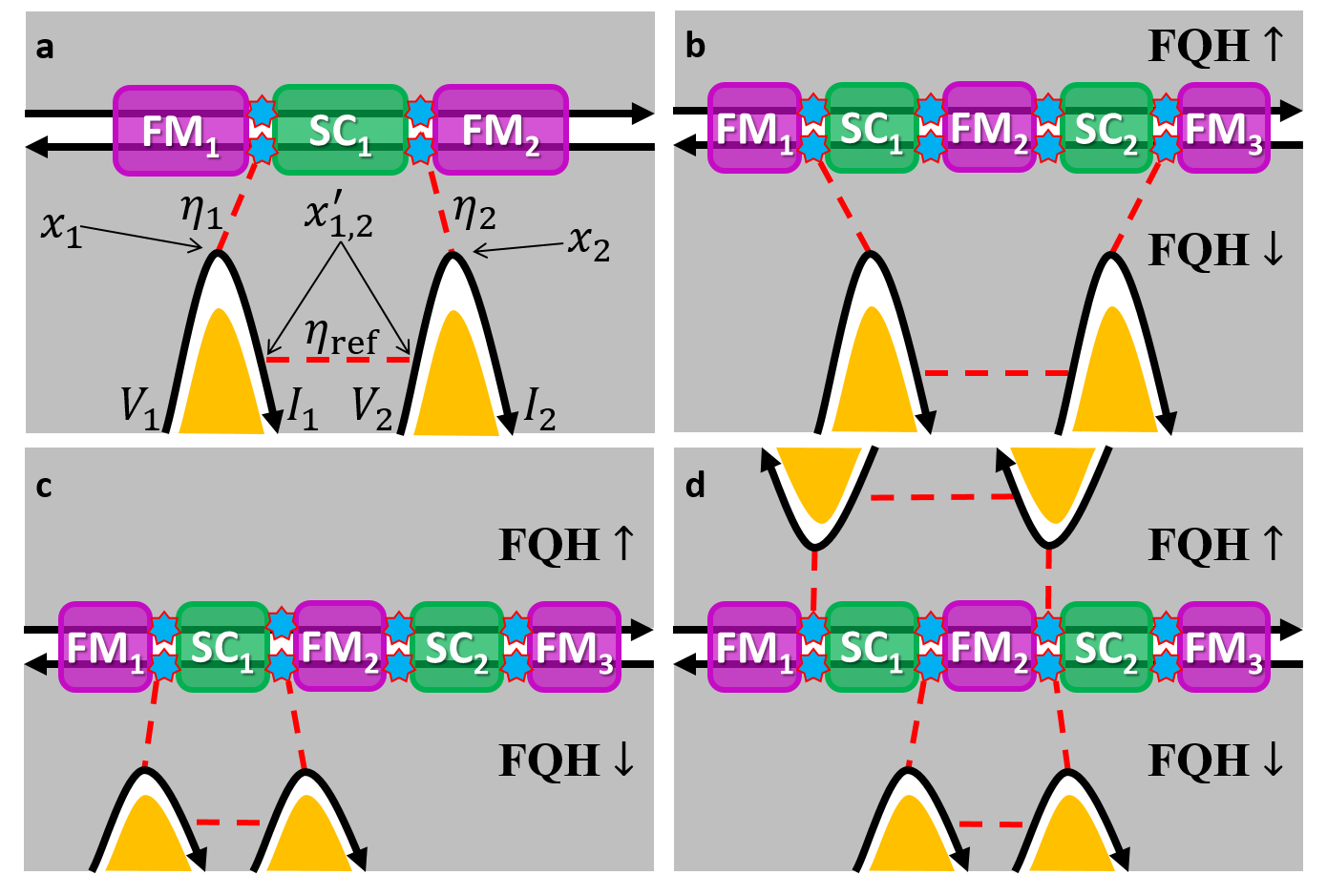
Figure 2: Setups for measuring the PF box state employing additional leads (FQH edges; the curved black arrows), tunnel couplings (the dashed red lines), and gates (golden) controlling the distance between the leads and the parafermions (and thus the strength of the tunnel couplings). (a) Measuring $\hat{Q}_{\mathrm{tot}}\leavevmode\nobreak\ \mathrm{mod}\leavevmode\nobreak\ 2$ in a one-box. (b,c,d) Setups for measuring various observables in a two-box: (b) $(\hat{Q}_{\mathrm{tot}}-\hat{S}_{2})\leavevmode\nobreak\ \mathrm{mod}\leavevmode\nobreak\ 2$; (c) $\hat{Q}_{1}\leavevmode\nobreak\ \mathrm{mod}\leavevmode\nobreak\ 2$; (d) $(\hat{S}_{2}-\hat{Q}_{1})\leavevmode\nobreak\ \mathrm{mod}\leavevmode\nobreak\ 2$ and $\hat{S}_{2}\leavevmode\nobreak\ \mathrm{mod}\leavevmode\nobreak\ 2$ for the upper and lower pairs of leads, respectively.

We now assume that the box charging energy in Eq. (9) is the largest energy scale. Away from Coulomb resonances $q_{\mathrm{g}}\neq\nu(\mathbb{Z}+1/2)$, transport between two leads is then dominated by cotunneling. Performing a Schrieffer–Wolff transformation and projecting to the state of $Q_{\mathrm{tot}}$ that minimizes the charging energy, $H_{\mathrm{box}}+H_{\mathrm{T}}\rightarrow H_{\mathrm{cot}}$, we obtain to the leading order,

$$H_{\mathrm{cot}}=\eta_{\mathrm{cot}}\hat{\alpha}_{j_{2},s}^{\thinspace}\hat{\alpha}_{j_{1},s}^{\dagger}e^{-i\sqrt{\nu}\hat{\phi}_{2}(x_{2})}e^{i\sqrt{\nu}\hat{\phi}_{1}(x_{1})}+\mathrm{H.c.},$$ (10)

where $\eta_{\mathrm{cot}}=-\eta_{1}\eta_{2}^{*}\left(U_{+}^{-1}+U_{-}^{-1}\right)$ with $U_{\pm}\sim E_{C}$ being the charging energy penalty for adding/removing one fractional quasiparticle to/from the box. The total Hamiltonian for transfer of quasiparticles between the leads is then given by

$$H_{\mathrm{T12}}=H_{\mathrm{T}}^{\mathrm{ref}}+H_{\mathrm{cot}}=\hat{\eta}_{\mathrm{T12}}e^{-i\sqrt{\nu}\hat{\phi}_{2}(x_{2})}e^{i\sqrt{\nu}\hat{\phi}_{1}(x_{1})}+\mathrm{H.c.},$$

$$\hat{\eta}_{\mathrm{T12}}=\eta_{\mathrm{ref}}+\eta_{\mathrm{cot}}\hat{\alpha}_{j_{2},s}^{\thinspace}\hat{\alpha}_{j_{1},s}^{\dagger}.$$ (11)

Since the operator $\hat{\alpha}_{j_{2},s}^{\thinspace}\hat{\alpha}_{j_{1},s}^{\dagger}$ in Eq. (11) acts only in the discrete box subspace, the effective cotunneling Hamiltonian $H_{\mathrm{T}12}$ corresponds to quasiparticle tunneling between the leads with effective amplitude $\hat{\eta}_{\mathrm{T12}}$. Noting that $(\hat{\alpha}_{j_{2},s}^{\thinspace}\hat{\alpha}_{j_{1},s}^{\dagger})^{n}=-1$ with $n=2/\nu$, one sees that the properties specific to PFs are encoded by the cotunneling phase. Indeed, the eigenvalues of $\hat{\alpha}{}_{j_{2},s}^{\thinspace}\hat{\alpha}_{j_{1},s}^{\dagger}$ follow as $e^{i\pi\nu(r+1/2)}$ (integer $r$), and the cotunneling phase therefore depends on the PF box state with possible phase values differing by multiples of $\pi\nu$.

Cotunneling current. Next we observe that $H_{\mathrm{T}12}$ is relevant under the renormalization group (RG) with scaling dimension equal to $\nu<1$ foot:scaling_dimension . The RG flow towards the strong quasiparticle tunneling regime eventually implies a two-terminal conductance $\nu e^{2}/h$ Kim2017 . However, for a finite voltage $V_{12}=V_{1}-V_{2}$ with $|V_{12}|\gg V_{B}\propto|\eta_{\mathrm{T12}}|^{1/(1-\nu)}$, the RG flow is effectively cut off. For a given $V_{12}$, this inequality is always realized for sufficiently small tunnel couplings. The tunneling current $I_{\mathrm{T}\mathrm{12}}=I_{2}-\nu e^{2}V_{2}/h$ between the two leads then follows from perturbation theory in $H_{\mathrm{T12}}$ Wen1991 ,

$$\hat{I}_{\mathrm{T}\mathrm{12}}=\frac{|\hat{\eta}_{\mathrm{T12}}|^{2}}{v^{2\nu}}\frac{2\pi\nu}{\Gamma(2\nu)}(\nu|V_{12}|)^{2\nu-1}\mathrm{sgn}(V_{12}),$$ (12)

$\Gamma(x)$ being the Euler gamma function. For a box initially in a superposition of different $\hat{\alpha}_{j_{2},s}^{\thinspace}\hat{\alpha}_{j_{1},s}^{\dagger}$ eigenstates, such a current measurement implies a projection to the observed eigenstate, cf. Refs. Landau2016 ; Plugge2017 . By measuring $\hat{I}_{\mathrm{T}\mathrm{12}}$ and hence $|\hat{\eta}_{\mathrm{T12}}|$, one can therefore characterize the quantum state of a PF box. In this calculation we assumed low temperatures ($T\ll|V_{12}|$) and long edges ($v/L\ll|V_{12}|$). Furthermore, we have put the points of direct tunneling between the two edges ($x_{1,2}^{\prime}$) to coincide with the points for tunneling to parafermions ($x_{1,2}$), cf. Fig. 2(a). Realistically, they will not coincide, resulting in a suppression of the interference term $\sim\eta_{\mathrm{cot}}\eta_{\mathrm{ref}}^{*}\hat{\alpha}_{j_{2},s}^{\thinspace}\hat{\alpha}_{j_{1},s}^{\dagger}+\mathrm{H.c.}$ which enables one to measure the eigenvalue of $\hat{\alpha}_{j_{2},s}^{\thinspace}\hat{\alpha}_{j_{1},s}^{\dagger}$. This suppression reduces (but does not destroy) the interference visibility.

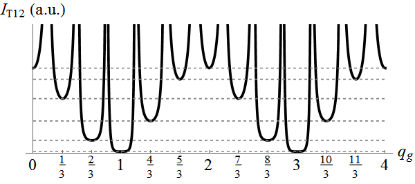
Figure 3: Sketch of the tunneling current $I_{\mathrm{T}\mathrm{12}}$ vs gate parameter $q_{\mathrm{g}}$ for the one-box configuration in Fig. 2(a) with $\nu=1/3$. The current in a Coulomb valley depends on $Q_{\mathrm{tot}}\leavevmode\nobreak\ \mathrm{mod}\leavevmode\nobreak\ 2$ and thus on $q_{\mathrm{g}}$. When gradually increasing $q_{\mathrm{g}}\rightarrow q_{\mathrm{g}}+2$, one passes through $n=2/\nu$ peaks with much stronger (yet finite) current. At the end of this sequence, the same current $I_{\mathrm{T}\mathrm{12}}$ is repeated.

Number of eigenvalues. Consider the configuration in Fig. 2(a), which gives access to the operator $\hat{\alpha}_{2,\downarrow}^{\thinspace}\hat{\alpha}_{1,\downarrow}^{\dagger}=e^{-i\pi(\hat{Q}_{\mathrm{tot}}+\nu/2)}$, cf. Eqs. (7) and (11), via two leads connected to a one-box. We now tune the box to a Coulomb-blockade valley. By varying the gate voltage across a peak $q_{\mathrm{g}}\rightarrow q_{\mathrm{g}}+\nu$, we also enforce $Q_{\mathrm{tot}}\rightarrow Q_{\mathrm{tot}}+\nu$ since the box will adhere to the ground state of $H_{\mathrm{box}}$. As a consequence, we effectively obtain $\eta_{\mathrm{cot}}\rightarrow\eta_{\mathrm{cot}}e^{-i\pi\nu}$ in Eq. (11) and thus a different tunneling current $I_{\mathrm{T}\mathrm{12}}$. After switching through $n=2/\nu$ subsequent Coulomb valleys, we have $q_{\mathrm{g}}\rightarrow q_{\mathrm{g}}+2$ and return to the original value of $I_{\mathrm{T}\mathrm{12}}$. This characteristic dependence of $I_{\mathrm{T}\mathrm{12}}$ on $q_{\mathrm{g}}$ is sketched in Fig. 3. Such an experiment can already determine the number $n$ of possible eigenvalues of $\hat{\alpha}_{2,\downarrow}^{\thinspace}\hat{\alpha}_{1,\downarrow}^{\dagger}$, which is a nontrivial check of the PF operator properties.

Degenerate PF space. Next we show how to engineer an $n$-fold degenerate PF space. To accomplish this task, we consider a two-box as shown in Figs. 2(b)–2(d). The two-box has two degrees of freedom, namely, $Q_{\mathrm{tot}}$, which behaves the same way as for the one-box, and $Q_{1}\leavevmode\nobreak\ (\mathrm{mod}\leavevmode\nobreak\ 2)$, which labels the $n$-fold degenerate subspace for any given $Q_{\mathrm{tot}}$. The two-box contains four domain walls, allowing for various options to access PF operator combinations. For instance, by connecting leads to the first and the last domain walls, cf. Fig. 2(b), a current measurement determines the phase of $\hat{\alpha}_{4,s}^{\thinspace}\hat{\alpha}_{1,s}^{\dagger}=e^{i\pi(s\hat{Q}_{\mathrm{tot}}+s\nu/2+\hat{S}_{2})}$. Repeating the above one-box protocol then implies a $q_{\mathrm{g}}$-dependent behavior as in Fig. 3. Next, we note that the subspace of fixed $Q_{\mathrm{tot}}$ is spanned by the $|Q_{1}\leavevmode\nobreak\ \mathrm{mod}\leavevmode\nobreak\ 2\rangle$ states. These states correspond to the eigenvalues $e^{is\pi(Q_{1}+\nu/2)}$ of $\hat{\alpha}_{2,s}^{\thinspace}\hat{\alpha}_{1,s}^{\dagger}$, which in turn follow from current measurements as shown in Fig. 2(c); $\hat{\alpha}_{3,s}^{\thinspace}\hat{\alpha}_{2,s}^{\dagger}=e^{i\pi(\hat{S}_{2}+s\nu/2)}$ and $\hat{\alpha}_{3,s}^{\thinspace}\hat{\alpha}_{1,s}^{\dagger}=e^{i\pi(s\hat{Q}_{1}+\hat{S}_{2}+s\nu/2)}$ implying that this degenerate subspace is also spanned by the eigenbasis of $\hat{S}_{2}$ or of $\hat{S}_{2}\pm\hat{Q}_{1}$. Both operators can be accessed as illustrated in Fig. 2(d). Now let us take any eigenstate $|Q_{1}\leavevmode\nobreak\ \mathrm{mod}\leavevmode\nobreak\ 2\rangle$ of $\hat{\alpha}_{2,s}^{\thinspace}\hat{\alpha}_{1,s}^{\dagger}$. Decomposing it into the eigenstates of $\hat{\alpha}_{3,s}^{\thinspace}\hat{\alpha}_{2,s}^{\dagger}$, we obtain

$$|Q_{1}\leavevmode\nobreak\ \mathrm{mod}\leavevmode\nobreak\ 2\rangle=\frac{1}{\sqrt{n}}\sum_{r=0}^{n-1}e^{i\pi\lambda_{r}}|(S_{2}\leavevmode\nobreak\ \mathrm{mod}\leavevmode\nobreak\ 2)=\nu r\rangle,$$ (13)

where $\lambda_{r}=r(Q_{1}\leavevmode\nobreak\ \mathrm{mod}\leavevmode\nobreak\ 2)$. Similar statements hold for any pair of the above observables. This structure allows one to confirm the degeneracy of the subspace.

Indeed, let us select an arbitrary pair of noncommuting bilinear PF operators, e.g., $\hat{O}_{1}=\hat{\alpha}_{2,\uparrow}^{\thinspace}\hat{\alpha}_{1,\uparrow}^{\dagger}$ and $\hat{O}_{2}=\hat{\alpha}_{3,\downarrow}^{\thinspace}\hat{\alpha}_{2,\downarrow}^{\dagger}$. A measurement of $\hat{O}_{1}$ now projects the box state onto one of its $n$ eigenstates. Then one measures $\hat{O}_{2}$, which should project the system with equal probabilities, see Eq. (13), onto any eigenstate of $\hat{O}_{2}$. Similarly, a subsequent measurement of $\hat{O}_{1}$ projects this state with equal probabilities onto one of the eigenstates of $\hat{O}_{1}$. Repeating this procedure many times, one can verify that $\hat{O}_{1}$ (or $\hat{O}_{2}$) has precisely $n$ possible eigenvalues. To explicitly check the degeneracy one may now proceed as follows. One first performs repetitive measurements of $\hat{O}_{1}$ with arbitrary time intervals between consecutive current measurements. If we always find the same eigenvalue, we know that $\left[\hat{O}_{1},H_{\mathrm{box}}\right]=0$. Now repeat this procedure for the operator $\hat{O}_{2}$, which does not commute with $\hat{O}_{1}$. If we also find $\left[\hat{O}_{2},H_{\mathrm{box}}\right]=0$, all eigenstates of both $\hat{O}_{1}$ and $\hat{O}_{2}$ have trivial time evolution, which proves the degeneracy of the PF space. We emphasize that checking the degeneracy and the size of the PF subspace is an important and nontrivial validation of the system properties.

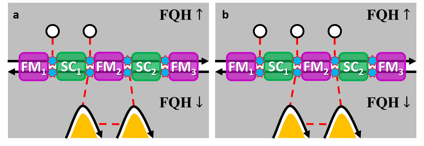
Figure 4: Setups allowing for two-box manipulation with QADs (the white circles). (a) The operator $\hat{\alpha}_{2,\uparrow}^{\thinspace}\hat{\alpha}_{1,\uparrow}^{\dagger}$ can be applied to an arbitrary PF box state by pumping a quasiparticle between the QAD pair. In the same setup, $\hat{S}_{2}\leavevmode\nobreak\ \mathrm{mod}\leavevmode\nobreak\ 2$ can be measured from the tunneling current between the shown leads. (b) A setup allowing for application of operations $\hat{\alpha}_{2,\uparrow}^{\thinspace}\hat{\alpha}_{1,\uparrow}^{\dagger}$ and $\hat{\alpha}_{3,\uparrow}^{\thinspace}\hat{\alpha}_{2,\uparrow}^{\dagger}$, which is sufficient to generate any digital operation that can be applied through QADs, and measuring $\hat{S}_{2}\leavevmode\nobreak\ \mathrm{mod}\leavevmode\nobreak\ 2$. Gates used to create QADs are kept implicit.

PF state manipulation. Finally we discuss how to perform on-demand transitions in the $n$-fold degenerate subspace of a two-box with QADs surrounded by the FQH liquid Kivelson1989 ; Kivelson1990 ; Goldman1996 ; Goldman1997 ; Maasilta1997 as access units, see Fig. 4. At low-energy scales, a QAD in the Coulomb-blockade regime is equivalent to a two-level system,

$$H_{\mathrm{QAD}}=\nu V_{\mathrm{QAD}}\left(\hat{\psi}_{\mathrm{QAD}}^{\dagger}\hat{\psi}_{\mathrm{QAD}}^{\thinspace}-\frac{1}{2}\right)=\frac{V_{\mathrm{QAD}}}{n}\begin{pmatrix}1&0\\ 0&-1\end{pmatrix},$$ (14)

where $V_{\mathrm{QAD}}$ is an electrostatic gate potential and $\hat{\psi}_{\mathrm{QAD}}$ is the quasiparticle annihilation operator on the QAD. Consider now two QADs coupled to the two-box as in Fig. 4(a). Similar to Eq. (11), elastic cotunneling between two QADs via the PF box is described by $H_{\mathrm{cot,QAD}}=\eta_{\mathrm{cot}}\hat{\psi}_{\mathrm{QAD2}}^{\dagger}\hat{\psi}_{\mathrm{QAD1}}^{\thinspace}\hat{\alpha}_{j_{2},s}^{\thinspace}\hat{\alpha}_{j_{1},s}^{\dagger}+\mathrm{H.c.}$, where the amplitude $\eta_{\mathrm{cot}}$ now does not renormalize anymore. By adiabatically pumping a quasiparticle from QAD1 to QAD2 through suitable changes in the gate voltages $V_{\mathrm{QAD1/2}}$, an arbitrary PF box state $|\Phi\rangle$ must then transform according to $|\Phi\rangle\rightarrow\hat{\alpha}_{j_{2},s}^{\thinspace}\hat{\alpha}_{j_{1},s}^{\dagger}|\Phi\rangle$. QADs thus facilitate digital operations $\hat{\alpha}_{j,s}^{\thinspace}\hat{\alpha}_{l,s}^{\dagger}$ within the degenerate PF subspace. Furthermore, employing protocols for both measurement with leads and manipulation with QADs, one can provide direct manifestations of the PF algebra (8); e.g., by measuring $\hat{\alpha}_{3,\downarrow}^{\thinspace}\hat{\alpha}_{2,\downarrow}^{\dagger}=e^{i\pi(\hat{S}_{2}-\nu/2)}$ and applying $\hat{\alpha}_{2,\uparrow}^{\thinspace}\hat{\alpha}_{1,\uparrow}^{\dagger}=e^{i\pi(\hat{Q}_{1}+\nu/2)}$ which shifts $\hat{S}_{2}\rightarrow\hat{S}_{2}-\nu\leavevmode\nobreak\ (\mathrm{mod}\leavevmode\nobreak\ 2)$, cf. Fig. 4(a). We emphasize that all nontrivial digital operations are generated by two operators, e.g., $\hat{\alpha}_{2,\uparrow}^{\thinspace}\hat{\alpha}_{1,\uparrow}^{\dagger}$ and $\hat{\alpha}_{3,\uparrow}^{\thinspace}\hat{\alpha}_{2,\uparrow}^{\dagger}$. These can be implemented with three QADs [Fig. 4(b)].

Conclusions. The parafermion box introduced in this Rapid Communication can simplify and facilitate experimental studies of PF-based quantum states. Our proposed measurement protocols, which employ fractional edge states as leads and/or quantum antidots for state manipulation, crucially rely on the unique and intrinsically nonlocal ways to access the box in the Coulomb-blockade regime. One can thereby largely avoid several difficulties that may affect earlier proposals for observing PF physics. In particular, we have shown how to observe the dimension of the zero-mode space, how to realize and demonstrate the existence of a degenerate space, and how to perform digital operations in this degenerate state manifold. The results of our protocols are distinctly different from Coulomb-blockade signatures of anyonic tunneling and should enable the experimental confirmation of the parafermion algebra in Eq. (8).

See pages ,1,,2,,3,,4,,5,,6,,7,,8 of ParafermionicBox_supplemental.pdf