Photon Correlations from the Mollow Triplet

Abstract

Photon correlations between the photoluminescence peaks of the Mollow triplet have been known for a long time, and recently hailed as a resource for heralded single-photon sources. Here, we provide the full picture of photon-correlations at all orders (we deal explicitly with up to four photons) and with no restriction to the peculiar frequency windows enclosing the peaks. We show that a rich multi-photon physics lies between the peaks, due to transitions involving virtual photons, and thereby much more strongly correlated than those transiting through the dressed states. Specifically, we show that such emissions occur in bundles of photons rather than as successive, albeit correlated, photons. We provide the recipe to frequency-filter the emission of the Mollow triplet to turn it into a versatile and tunable photon source, allowing in principle all scenarios of photon emission, with advantages already at the one-photon level, i.e., providing more strongly correlated heralded single-photon sources than those already known.

I Introduction

Resonance fluorescence is one of the simplest and yet most fruitful case of light-matter interaction. It describes the emission of a two-level system (2LS) that is driven coherently and at the same frequency than it emits vogel_book06a . Following the prediction of its antibunching emission carmichael76a , it provided the first direct evidence of quantization of the light field kimble77a (the photo-electric effect, that suggests it, could also be explained semi-classically). The interferences between the absorbed and emitted light result in counter-intuitive effects heitler_book44a ; lopezcarreno16b that power one of the best mechanism for single-photon emission, currently under fervent development aharonovich16a . Of particular interest is the high excitation regime, described theoretically by Benjamin Mollow in 1969 mollow69a and first observed by crossing at right angle a low-density gas of sodium atoms with a dye laser beam at resonance with a two-level Na transition (the $F=2\rightarrow 3$ hyper-fine transition of the $D_{2}$ line) schuda74a , an observation since then repeated in a wealth of other platforms keitel95a ; bienert04a ; bienert07a ; flagg09a ; astafiev10a ; makhonin14a ; toyli16a ; unsleber16a ; lagoudakis17a . The appeal of this high-driving fluorescence comes from its peculiar spectral lineshape, that takes the form of a triplet (shown in Fig. 1).

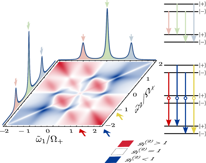
Figure 1: (Color online). The Mollow triplet (spectral lineshape) and its two-photon correlation spectrum (density plot) with the Mollow ladder of dressed states (right) whose transitions between manifolds account for the main phenomenology: power spectrum at the one-photon level and two-photon spectrum when jumping over intermediate manifolds through “leapfrog processes”. The density plot was obtained setting the decay rate of the 2LS as the unit, $\Omega=5\gamma_{\sigma}$, $\Gamma=\gamma_{\sigma}$ and setting the laser in resonance with the 2LS. The color code is red for $g_{\Gamma}^{(2)}>1$, white for $g_{\Gamma}^{(2)}=1$ and blue for $g_{\Gamma}^{(2)}<1$, with the deepest red (blue) set to the maximum (minimum) value.

The most elegant physical interpretation of this triplet describes the system as dressed by the laser cohentannoudji77a ; reynaud83a . This gives rise to new eigenstates $\left|\pm\right\rangle$, whose transitions account for the main features: a triplet in which the integrated spectral intensities of its peaks have 1:2:1 proportions (when the laser is resonant with the transition). This is shown in the upper part of the ladder of dressed state in Fig. 1. The properties of these new states have been studied early on, with a good quantitative description from the dressed state picture, assuming spontaneous emission events between the eigenstates of the combined laser-atom system. Apanasevich and Kilin apanasevich79a first computed in this framework the photon correlations between the peaks and predicted most of their qualitative cross-correlations, such as antibunching of the side peaks emission and bunching for cross-peaks emission. Following similar (and independent) theoretical predictions from Cohen Tannoudji and Reynaud cohentannoudji79a , Aspect et al. aspect80a measured such photon correlations between the sidebands, and observed the radiative cascade and time-ordering so naturally explained by the dressed atom picture alhilfy85a . Schrama et al. schrama91a ; schrama92a extended the theory to the regime of small correlation times, which requires to take into account interferences between the various emitted photons, resulting for instance in antibunching between a side-peak and satellite photon, instead of uncorrelated emission as predicted by the earlier theories. They obtained excellent quantitative agreement with correlations measured from the resonance fluorescence of the ${}^{1}S_{0}\rightarrow{}^{1}P_{1}$ transition in barium, albeit after several type of corrections to take into account experimental limitations. This has remained the state of the art until the recent re-emergence of this problem in the solid state, with Ulhaq et al. ulhaq12a ’s revisiting of the photon correlations between the peaks from a the resonance fluorescence of an In(Ga)As quantum dot. In this and previous experiments as well as in the bulk of the theoretical efforts, the photon correlations have thus been limited to photons from the peaks. Meanwhile, the formal theories of frequency-resolved photon correlations led to increasingly better but also more intricate models that involve heavy computations to accommodate all the time-orderings of the emitted photons arnoldus84a ; knoll84a ; nienhuis93a , in particular if expanding the correlations to higher numbers of photons knoll86a , and this was typically tackled through approximations relying on the dressed state picture, which also constrained the computations to the peaks.

A recent theory of frequency-resolved photon correlations delvalle12a relaxes these restrictions and permits an exact treatment, to high photon numbers and for any spectral windows. In the most popular case of two-photon correlations, this readily provides the full landscape of all correlations between all combinations of frequencies, enclosing or not the peaks gonzaleztudela13a ; delvalle13a . This two-photon correlation spectrum, shown in Fig. 1, unravels a rich structure, with another triplet of lines, this time at the two-photon level, corresponding to direct transitions from one manifold to two below, jumping over the intermediate one in a “leapfrog process”, sketched in the bottom of the ladder in Fig. 1. The intermediate photon in this process is virtual (represented by $\circ$), resulting in strong correlations of the emitted pair sanchezmunoz14b . This two-photon spectrum has been measured by Peiris et al. peiris15a , showing how the correlations between the peaks that had been known since the early years of the Mollow triplet, were particular cases of a wider picture.

In this text, we provide an exact description of high-order photon correlations from the Mollow triplet and propose configurations that extend the realm of possible experiments and applications that have been explored so far by correlating the peaks, replacing real-state transitions by strongly-correlated leapfrog processes. We also review the state of the art as we introduce notations and main formalism.

II Spectral shape of the Mollow triplet

The Mollow triplet is the photoluminescence lineshape of a two-level system (2LS) driven strongly by a coherent source, as described by the Hamiltonian (we use $\hbar=1$ along the paper)

$$H_{\sigma}=(\omega_{\sigma}-\omega_{\mathrm{L}}){\sigma^{\dagger}}\sigma+\Omega({\sigma^{\dagger}}+\sigma)\,,$$ (1)

where $\sigma$ is the annihilation operator of the 2LS with free energy $\omega_{\sigma}$, with the coherent driving described by the $c$-number $\Omega$ (amplitude of a classical field) and its energy $\omega_{\mathrm{L}}$ (absorbed in the 2LS free energy once in the rotating frame). The dissipative character of the system is taken into account through the master equation

$$\partial_{t}\rho=i[\rho,H_{\sigma}]+\frac{\gamma_{\sigma}}{2}\mathcal{L}_{\sigma}\rho\,,$$ (2)

where $\gamma_{\sigma}$ is the 2LS decay rate and $\mathcal{L}_{c}\equiv 2c\rho{c^{\dagger}}-{c^{\dagger}}c\rho-\rho{c^{\dagger}}c$. When the system enter the strong coupling regime, which is the case we shall consider from now onward (although not a restriction for the formalism), the spectrum consists of three Lorentzians split by

$$\Omega_{+}\equiv\frac{\sqrt{8\Omega_{0}^{2}-6\gamma_{\sigma}^{2}+\sqrt{9\gamma_{\sigma}+16\Omega_{0}^{4}-24\gamma_{\sigma}^{2}(16\Omega^{2}+\Omega_{0}^{2})}}}{2\sqrt{3}}\,,$$ (3)

where $\Omega_{0}^{2}=4\Omega^{2}+\tilde{\omega}_{\sigma}^{2}$ (so that in the limit $\Omega_{0}\gg\gamma_{\sigma}$, the splitting is simply $\Omega_{+}\approx\Omega_{0}$). The two sidebands have the same spectral weight while the central one decreases with detuning from twice as large at resonance to zero when $\tilde{\omega}_{\sigma}\gg\gamma_{\sigma}$.

While the spectral shape is readily obtained by solving the master equation, it is better understood on physical grounds as transitions between the eigenstates $\left|\pm\right\rangle=\left|\mathrm{e},n\right\rangle\pm\left|\mathrm{g},n-1\right\rangle$ of the 2LS (with basis states $\left|\mathrm{g}\right\rangle$, $\left|\mathrm{e}\right\rangle$) coupled to $n$-photons from the driving laser. For $n\gg 1$—the case of strong-driving—the splitting between $\left|+\right\rangle$ and $\left|-\right\rangle$ does not depend appreciably on $n$. The level structure of an infinite ladder of manifolds separated by the energy of the laser and each split by $\Omega_{+}$, pervades the phenomenology of resonance fluorescence in the high-excitation regime. The immediate insight brought by the one-photon transitions—the central peak having twice the weight because two of the four transitions are degenerate—shows that this is a powerful tool to guide one’s intuition. For instance, the transitions that yield the central peak, $\left|\pm\right\rangle\rightarrow\left|\pm\right\rangle$, leave the state of the 2LS unchanged, while those that yield the side peaks, $\left|\pm\right\rangle\rightarrow\left|\mp\right\rangle$, change the state of the 2LS. As detuning changes the light-matter composition of the state, it is an important degree of freedom to tune the triplet’s properties, as we will see in the following. In some regime, the dressed-atom description even becomes exact reynaud83a and quantitative results can be obtained through rate equations for the transitions between the states. Early on, it was appreciated on the basis of this picture that subsequent cascades between dressed states result in photon correlations. The basic reasoning is equally simple. For instance, the cascade $\left|+\right\rangle\rightarrow\left|+\right\rangle\rightarrow\left|+\right\rangle$ (id. with $-$) leads to bunching from the $\left|+\right\rangle\rightarrow\left|+\right\rangle$ transition, that corresponds to the central peak. In contrast, $\left|+\right\rangle\rightarrow\left|-\right\rangle$ or $\left|-\right\rangle\rightarrow\left|+\right\rangle$ cannot happen in succession, leading to antibunching of these transitions (the side peaks). Slightly more careful analysis to take into account interferences between the various possible paths, also explains along these lines why side and central peaks are antibunched schrama91a .

III Leapfrog processes

Another class of transitions takes place in the same ladder, that has been overlooked until its identification in the two-photon spectrum by Gonzalez Tudela et al. gonzaleztudela13a . It consists of transitions from one real state to another but involving two photons $\left|+\right\rangle\rightrightarrows\left|-\right\rangle$, three $\left|+\right\rangle\mathrel{\vbox{\offinterlineskip\hbox{$\rightarrow$}\vskip 0.43057pt\hbox{$\rightarrow$}\vskip 0.43057pt\hbox{$\rightarrow$}}}\left|-\right\rangle$ or any number, jumping over as many manifolds as there are many photons involved. The difference between $\left|+\right\rangle\rightarrow\left|\pm\right\rangle\rightarrow\left|-\right\rangle$ and $\left|+\right\rangle\rightrightarrows\left|-\right\rangle$ is that in the former case, each photon is real, with the first transition taking place independently from the second. The correlations are thus of a classical character: the second transition is likely, because the first one reached the state that allows the second to take place. Something else, however, could happen. In the latter case, there is one transition only, so that it happens with the two photons emitted simultaneously, with stronger correlations as the joint emission is intrinsic to the process delvalle11d . The latter case also allows to relax the conditions on the photons: their individual energies do not need to match any allowed transition, only their sum does. This provides the simple equations for the two-leapfrog processes:

$$\tilde{\omega}_{1}+\tilde{\omega}_{2} =0\,,$$ (4a)

$$\tilde{\omega}_{1}+\tilde{\omega}_{2} =\Omega_{+}\,,$$ (4b)

$$\tilde{\omega}_{1}+\tilde{\omega}_{2} =-\Omega_{+}\,,$$ (4c)

where $\tilde{\omega}_{i}\equiv(\omega_{i}-\omega_{\mathrm{L}})$ for $i=1,2$. These direct counterparts of the Mollow triplet transitions at the two-photon level are the antidiagonal lines of superbunching, $g^{(2)}\gg 1$, seen in Fig. 1. While the conditions Eqs. (4) can also be satisfied by photons from real transitions, this breaks the tie by transforming one virtual photon into a real one when transiting by the intermediate manifold.

This mechanism can be generalized to transitions involving $N$ photons:

$$\tilde{\omega}_{1}+\tilde{\omega}_{2}+\cdots+\tilde{\omega}_{N}=\Delta\,,\text{ with~{}$\Delta=-\Omega_{+},0,\Omega_{+}$}\,.$$ (5)

Here as well, Eq. (5) can be met by matching real transitions, with any number from one to all the intermediate photons. The most strongly correlated case corresponds to all intermediate photons being virtual, in which case we refer to a “$N$-photon leapfrog”, hopping over $N-1$ intermediate manifolds.

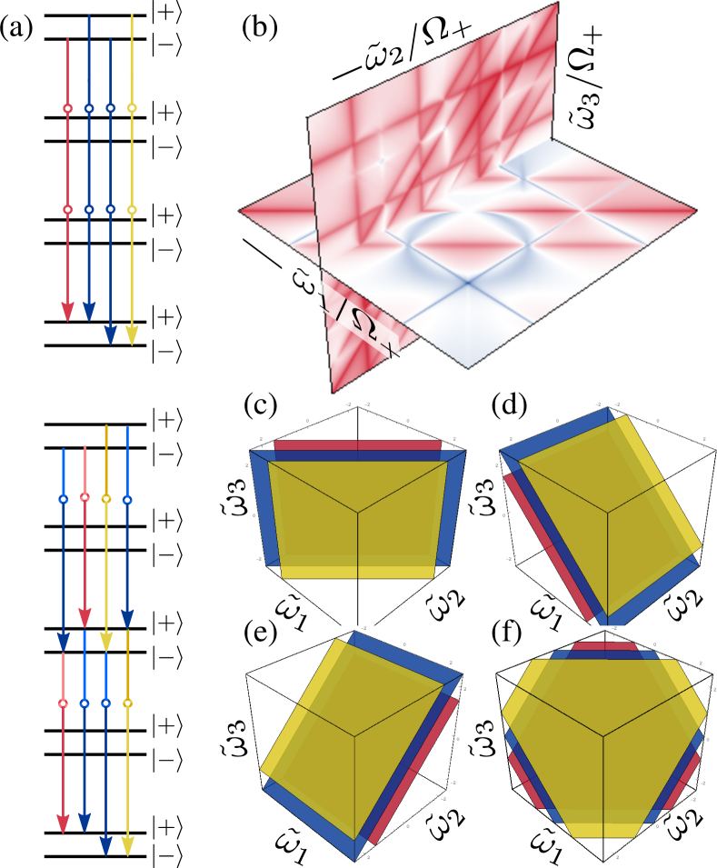
Figure 2: (Color online). Third order correlation function $g^{(3)}_{\Gamma}(\omega_{1},\omega_{2},\omega_{3})$. The various transitions sketched in Panel (a) give rise to a rich landscape of correlations as shown in Panel (b) through a two-plane cut in the full-3D structure. The vertical plane is pinned at a leapfrog transition while the horizontal plane is pinned at the central peak. The color code is blue for $g^{(3)}_{\Gamma}<1$, white for $g^{(3)}_{\Gamma}=1$ and red for $g^{(3)}_{\Gamma}>1$. The antidiagonals of superbunching are given by the intersections with the leapfrog planes given by Eqs. (6), displayed in panels (c-f). The colors correspond to the different values for $\Delta$ there, namely $\Omega_{+}$ (shown in yellow), $0$ (blue) and $-\Omega_{+}$ (red). Panel (b) was obtained for the decay rate of the 2LS as the unity, $\Omega_{+}=300\gamma_{\sigma}$, $\tilde{\omega}_{\sigma}=200\gamma_{\sigma}$ and $\Gamma=5\gamma_{\sigma}$.

As characteristic of a quantum system, the combinatorics aspect quickly becomes overriding in the description of the phenomenology. At the two-photon level, the picture is fully captured by the two-photon spectrum, that has been already widely discussed gonzaleztudela13a ; sanchezmunoz14b ; gonzaleztudela15a ; peiris15a ; peiris17a . We thus consider next the three-photon level. The standard correlation function is that provided by Glauber for the general case glauber63a , namely, $g^{(3)}$. With frequency filtering, this becomes $g^{(3)}_{\Gamma_{1},\Gamma_{2},\Gamma_{3}}(\omega_{1},t_{1};\omega_{2},t_{2};\omega_{3},t_{3})$. Assuming the same filter linewidths $\Gamma$ and considering coincidences only, $t_{1}=t_{2}=t_{3}=0$, we arrive at a 3D correlation spectrum $g^{(3)}_{\Gamma}(\omega_{1},\omega_{2},\omega_{3})$, that is shown in Fig. 2 (the details of its computation are given in next Section). It is not easy to visualize a three-dimensional correlation structure, but we can nevertheless characterize it fairly comprehensively. It consists essentially of leapfrog planes of superbunching, which, following Eqs. (5), read at the three-photon level:

$$\tilde{\omega}_{1}+\tilde{\omega}_{2}=\Delta\,,$$ (6a)

$$\tilde{\omega}_{1}+\tilde{\omega}_{3}=\Delta\,,$$ (6b)

$$\tilde{\omega}_{2}+\tilde{\omega}_{3}=\Delta\,,$$ (6c)

$$\tilde{\omega}_{1}+\tilde{\omega}_{2}+\tilde{\omega}_{3}=\Delta\,,$$ (6d)

where $\Delta$ is one of the three combinations of initial/final states transitions, i.e., $\Delta=-\Omega_{+}$ (the red planes in Fig. 2(c–f)), $\Delta=0$ (blue) and $\Delta=\Omega_{+}$ (yellow). The planes from Eq. (6d) are the three-photon leapfrogs, where all the intermediate photons are virtual, as shown in the upper part of the Mollow ladder in Fig. 2(a). The planes from Eqs. (6a–6c) correspond to three-photon correlations that involve two two-photon leapfrog transitions linked by a radiative cascade, namely, with two photons belonging to one two-photon leapfrog transition while the third comes from another two-photon leapfrog transition. Alternatively, this can be seen as a four-leapfrog transition that intersects a real-state, breaking it in two two-leapfrog transitions. This is shown in the bottom of the ladder in panel (a). It is at this point that the concept introduced by Sanchez Muñoz et al. sanchezmunoz14b of a “bundle”—the $N$-photon object issued by a leapfrog transition—becomes handy. The planes in panels (c–e) thus correspond to a bundle-bundle radiative cascade in the Mollow ladder, the exact same process as that discussed by Cohen-Tannoudji & Reynaud in the dressed-atom picture, but for two-photon bundles instead of individuals photons. The plane in panel (f) correspond to a single three-photon bundle transition.

Before turning to exact calculations, we illustrate how the powerful dressed-atom picture also allows us to make some qualitative statements on the expected behaviours at the bundle level. For instance, considering $N$-photon bundles where all photons have the same energy, i.e., with bundle frequency $\pm\Omega_{+}/N$, we can anticipate them to be pairwise bunched. In contrast, since the degenerated $N$-photon leapfrog transitions need to change the state of the 2LS, for otherwise they break into real-state transitions, two identical $N$-photon bundles cannot be emitted consecutively, and therefore their pairwise correlations should be anti-correlated. Note that one expects such a behaviour at the level of the bundles rather than at the level of the photons themselves, that should be bunched in all cases.

To get a more quantitative picture, we need to turn to an exact theory of frequency-resolved three-photon correlations, that we present in next Section. Importantly, this will confirm that the leapfrog transitions (6) are the main three-photon relaxation processes. Every red line in panel (b) is accounted for by one of the planes in panels (c–f). This remains true for any other cuts in the 3D structure (to assist in the visualization of this three-photon correlation spectrum, we also provide an animated version as Supplementary Material). The case of a real transition followed by a leapfrog transition is a particular case that traces a line in the 3D structure, that is absorbed in one of the planes. In this sense, the anatomy of three-photon correlations is captured by the leapfrog planes and therefore remains relatively simple to comprehend.

IV Theory of frequency-resolved $N$ photon correlations

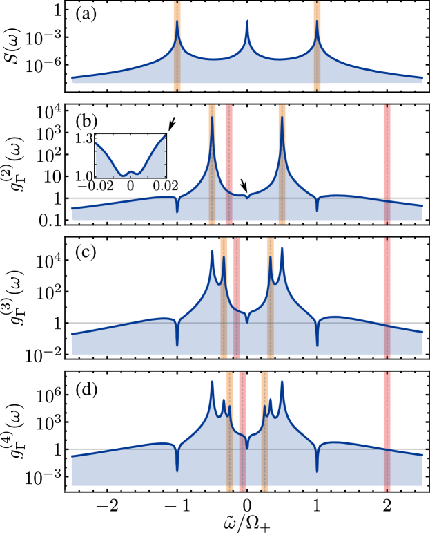
Figure 3: (Color online). Correlation among bundles of $N$ photons. (a) Single photon heralding as proposed in Ref. schrama92a, . (b-d) The resonances in the photon correlations reveal the frequencies where the same type of heralding but for $N$-photon bundles can be achieved. Such frequencies, shown here in yellow, are given by $\tilde{\omega}=\pm\Omega_{+}/N$ at order $N$. In red are shown the even better configuration where the heralding does not involve any transition through a real state. The inset in Panel (b) shows a zoom of the correlations nearby the central peak, marked by an arrow, revealing bunching to sit on a local minimum. The decay rate of the 2LS sets the unit, the splitting of the triplet is set to $\Omega_{+}=300\gamma_{\sigma}$, the sensors linewidth to $\Gamma=2\gamma_{\sigma}$, and the detuning between the laser and the 2LS to $\tilde{\omega}=200\gamma_{\sigma}$.

The correlations between $N$ photons detected in as many (possibly degenerate) frequency windows as required, without restricting ourselves to the peaks, are obtained with the theory of frequency-resolved correlations of del Valle et al. delvalle12a . In this formalism, one computes correlations between $N$ “sensors” (in the simplest case, each sensor is a 2LS), at the frequencies $\omega_{k}$ to be correlated. Sensors correlations are then computed in the limit of their vanishing coupling $\epsilon$ to the system (in this text, the resonantly fluorescing 2LS). The Hamiltonian describing such a coupling for the problem at hand is

$$H_{\xi_{k}}=\tilde{\omega}_{k}{\xi_{k}^{\dagger}}\xi_{k}+\epsilon({\sigma^{\dagger}}\xi_{k}+{\xi_{k}^{\dagger}}\sigma)\,,$$ (7)

where $\xi_{k}$ is the annihilation operator of the $k$th sensor and $\tilde{\omega}_{k}=\omega_{k}-\omega_{\mathrm{L}}$ is the detuning between the sensor and the driving laser. The spectral width of the filters enters in the formalism as the sensors decay rate $\Gamma_{k}$. The complete master equation of the 2LS supplemented with the set of sensors then reads

$$\partial_{t}\rho=i\left[\rho,H_{\sigma}+\hat{H}_{\mathrm{\xi}}\right]+\frac{\gamma_{\sigma}}{2}\mathcal{L}_{\sigma}\rho+\frac{1}{2}\hat{\mathcal{L}}_{\xi}\rho\,,$$ (8)

where $\hat{H}_{\xi}=\sum_{k}H_{\xi_{k}}$ and $\hat{\mathcal{L}}_{\xi}\rho=\sum_{k}\Gamma_{k}\,\mathcal{L}_{\xi_{k}}\rho$, with the summation over as many sensors as required for the order of the correlation ($N$ sensors for $g^{(N)}$). The two- (Fig. 1) and three-photon (Fig. 2) frequency-resolved correlations are thus computed as

$$g_{\Gamma}^{(2)}(\tilde{\omega}_{1},\tilde{\omega}_{2})=\frac{\langle{\xi_{1}^{\dagger}}(\tilde{\omega}_{1}){\xi_{2}^{\dagger}}(\tilde{\omega}_{2})\xi_{2}(\tilde{\omega}_{2})\xi_{1}(\tilde{\omega}_{1})\rangle}{\langle{\xi_{1}^{\dagger}}(\tilde{\omega}_{1})\xi_{1}(\tilde{\omega}_{1})\rangle\langle{\xi_{2}^{\dagger}}(\tilde{\omega}_{2})\xi_{2}(\tilde{\omega}_{2})\rangle}\,,$$ (9a)

$$g_{\Gamma}^{(3)}(\tilde{\omega}_{1},\tilde{\omega}_{2},\tilde{\omega}_{3})=\\ \frac{\langle{\xi_{1}^{\dagger}}(\tilde{\omega}_{1}){\xi_{2}^{\dagger}}(\tilde{\omega}_{2}){\xi_{3}^{\dagger}}(\tilde{\omega}_{3})\xi_{3}(\tilde{\omega}_{3})\xi_{2}(\tilde{\omega}_{2})\xi_{1}(\tilde{\omega}_{1})\rangle}{\langle{\xi_{1}^{\dagger}}(\tilde{\omega}_{1})\xi_{1}(\tilde{\omega}_{1})\rangle\langle{\xi_{2}^{\dagger}}(\tilde{\omega}_{2})\xi_{2}(\tilde{\omega}_{2})\rangle\langle{\xi_{3}^{\dagger}}(\tilde{\omega}_{3})\xi_{3}(\tilde{\omega}_{3})\rangle}\,,$$ (9b)

with an obvious generalization to higher orders. Importantly, the normalization cancels the $\epsilon$ coupling, so that the result is a fundamental property of the system, only dependent on the filter linewidths—as is mandatory from the time-energy uncertainty—but otherwise independent from detectors efficiencies, coupling strengths, time of acquisition, etc.

A particular case of interest is the autocorrelation $g^{(N)}(\tilde{\omega})$ when all the frequencies are degenerate, $\tilde{\omega}_{1}=\cdots=\tilde{\omega}_{N}$. This corresponds to the correlations, at various orders, of the light passing through a single filter. Exact computations of these configurations as obtained by the sensors technique are shown in Fig. 3. Panel (b) confirms the known results aspect80a ; schrama92a ; ulhaq12a obtained in the literature of antibunching for the side peaks, and also of bunching for the main peak ($g^{(2)}_{\Gamma}(0)\approx 1.05$ with our parameters, see caption). Strikingly in the latter case, it is revealed that this bunching actually sits in a local minimum and that in the full picture, although the central peak is indeed bunched, this comes as a local maximum in a region of suppressed bunching, as shown in the inset of Fig. 3(b) (zooming in the area indicated by the arrow). This feature is not fully conveyed by the dressed atom picture. The most notable feature is one that remained unnoticed until recently gonzaleztudela13a : the two strong resonances that sit between the peaks. These are the leapfrog correlations. Similar results are generalized when turning to higher orders, as shown in panels (c) (three photons) and (d) (four photons). While the correlation of the peaks retain the same qualitative behaviours, new features thus appear away from the peaks, associated to the leapfrog transitions, successively captured by increasing the order of the correlations. These resonances, at $\pm\Omega_{+}/N$, pile up toward the central peak, and become increasingly difficult to access individually, as however can be expected from such strongly quantum objects involving a large number of particles.

While these cuts in $N$th-order correlation spectrum are useful and will be later referred to again—being so-closely connected to degenerate bundles—they provide a very simplified account of the structure of the correlations at the $N$-photon level. The full picture for $N=3$ is displayed in Fig. 2(b), in two planes that intersect the full 3D spectrum (the Supplementary Video shows how these intersections scan through the full structure). The intersectiong with the leapfrog planes, from panels (c–f), results in red superbunching lines. We do not discuss the antibunching patterns (intersected as a blue circle) revealed by the computation, that is still of unclear physical origin and is not relevant for the points of this text.

V Sources of heralded photons

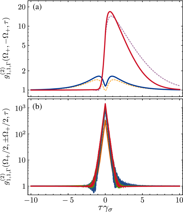
Figure 4: (Color online). Filtered single-photon correlations from the emission of, (a) the opposite sidebands, and, (b) the two-photon leapfrogs. Panel (a) shows the exact behaviour at resonance (blue) and with detuning (red), and compares it with the approximated expressions given in Ref. schrama92a , shown here as dashed orange and dashed purple, respectively. Panel (b) shows the filtered correlations from the same two-photon leapfrog (shown in red at resonance and in green with detuning) and from the leapfrogs at opposite sides of the central peak (shown in orange at resonance and in blue with detuning). The decay rate of the 2LS sets the unit, $\Omega_{+}=300\gamma_{\sigma}$, $\Gamma=5\gamma_{\sigma}$ and in the cases with detuning $\tilde{\omega}_{\sigma}=200\gamma_{\sigma}$.

With this formalism, it is straightforward to compute the exact frequency-resolved peak-peak correlations that have been studied by Ulhad et al. ulhaq12a . This is shown in Fig. 4(a) for the correlations in time, at both resonance (blue curve) and with laser detuning (red curve). We compare the exact (solid) and approximated (dotted) solutions, obtained through the sensing formalism or the earlier theories, respectively, with an excellent qualitative if not quantitative agreement. In the case of laser detuning, the asymmetric shape lends itself to heralding purposes, whereby detection of a photon from the high-energy peak correlates strongly with the detection of another photon from the low-energy peak. This is a useful resource for quantum sources of light (in particular single-photon sources).

The great advantage of the theory of frequency-resolved photon correlations is that it also allows to compute exactly correlations in more general configurations than those restricted to the peaks. For instance, correlating the leapfrog processes, one get the correlation function shown in Fig. 4(b), with several notable features, all in line with the quantum nature of these transitions: 1) the correlations are much stronger (about 50 times), 2) they have smaller correlation time (and thus yield better time resolutions), 3) they do not depend much on detuning, 4) they do not depend much on the choice of configuration (degenerate bundles or not) and 5) they are symmetric in time. Note that the symmetric correlation do not appear to be detrimental for heralding, as the instantaneous (within a reduced time window) character of the emission allows to delay one channel and thus keep the other as the heralding one. One obvious drawback of such strongly-correlated emission is the much reduced signal, since the collection is made away from the peaks. While there are ways to circumvent this limitation, for instance by Purcell enhancing them with a cavity of matching frequency delvalle13a ; sanchezmunoz14a ; sanchezmunoz15a , we will remain here at the level of describing the naked correlations. Now that we have shown the new perspectives opened by the leapfrog process at the two-photon level, we focus on more innovative aspects.

VI Sources of heralded bundles

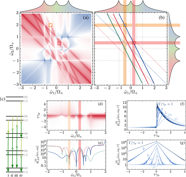
Figure 5: (Color online). Correlations between a single photon and a bundle of two photons. Panel (a) displays the structure of the correlations $g_{1,2,\Gamma}^{(2)}(\omega_{1},\omega_{2})$ between a a single photon with frequency $\omega_{2}$ and a bundle of two photons, each with frequency $\omega_{1}$. The antidiagonals featuring high correlations are shown in Panel (b): the dashed lines correspond to the transitions $\tilde{\omega}_{1}+\tilde{\omega}_{2}=\Delta$, whereas the solid lines correspond to the transitions $2\tilde{\omega}_{1}+\tilde{\omega}_{2}=\Delta$. The latter are shown in the ladder in Panel (c), where the dark green arrows represent the two-photon bundles and the light green arrows the single photon. Panel (e) shows the correlations profile of the solid antidiagonals in (b). In particular, the correlations between two-photon bundles emitted at $\tilde{\omega}_{1}=-\Omega_{+}/2$ (corresponding to the blue antidiagonal and displayed here within the orange filter) are bunched, they actually correspond to a local minimum. The global maximum, on the other hand, lies at an unremarkable frequency, at the location of the red filter. Panel (d) shows the $\tau$-dynamics across the blue antidiagonal, and the profiles from the time-correlations measured by the orange and red filters are displayed in Panels (f) and (g), respectively. Although the correlations in panel (f) have the $\lambda$-shape commonly associated to photon heralding, the correlations in Panel (g) are much stronger. The triplet splitting is $\Omega_{+}=300\gamma_{\sigma}$, the detuning between the laser and the 2LS is $\tilde{\omega}_{\sigma}=200\gamma_{\sigma}$ and, unless stated otherwise, the spectral width of the sensors is $\Gamma=5\gamma_{\sigma}$.

The powerful dressed-atom picture allows a straightforward generalization of the heralding discussed in the previous Section. One can contemplate the configuration where a photon heralds a bundle in the radiative cascade down the ladder, as shown in case $i$ of Fig. 5(c). This is the same idea as Ulhaq et al.’s heralding a single-photon, but now heralding a bundle instead. Even better, however, is to consider a three-photon leapfrog where all photons are virtual, and use one of them to herald the other two, a sketched in case $ii$. Conveniently, one can use the heralding photon to have a different energy from the two other ones, that can be degenerate. One needs a careful analysis, however, since there is room for subtleties in a relaxation process that starts to be complex. As an illustration, case $ii$, that has no real photons, has in fact the same distribution of photon frequencies as case $i$, that transits via a real state. The difference is the initial and final states, $\left|-\right\rangle\rightarrow\left|+\right\rangle\rightrightarrows\left|-\right\rangle$ and $\left|+\right\rangle\mathrel{\vbox{\offinterlineskip\hbox{$\rightarrow$}\vskip 0.43057pt\hbox{$\rightarrow$}\vskip 0.43057pt\hbox{$\rightarrow$}}}\left|+\right\rangle$. For this reason, case $ii$ turns out to be suppressed as a three-photon leapfrog process, as revealed by the exact calculation. One needs instead to find a case such as $iii$ that suffers no such interference with another relaxation in the ladder that intersects with a real state. A quantitative analysis is thus required, and the theory of frequency-resolved photon correlations delvalle12a here again allows us to easily tackle this problem. The relevant correlation is the one that generalizes Eq. (9a) to the $N$-th order correlation function of $N$ bundles, with each of them—detected at frequency $\tilde{\omega}_{\mu}$—being composed of $n_{\mu}$ photons:

$$g_{{n_{1}},\cdots,{n_{N}},\Gamma}^{(N)}(\tilde{\omega}_{1},\dots,\tilde{\omega}_{N})\equiv\frac{\langle:\Pi_{\mu=1}^{N}{\xi_{\mu}^{\dagger}}^{n_{\mu}}(\tilde{\omega}_{\mu})\xi_{\mu}^{n_{\mu}}(\tilde{\omega}_{\mu}):\rangle}{\Pi_{\mu=1}^{N}\langle{\xi_{\mu}^{\dagger}}^{n_{\mu}}(\tilde{\omega}_{\mu})\xi_{\mu}^{n_{\mu}}(\tilde{\omega}_{\mu})\rangle}\,,$$ (10)

where “$:$” indicates normal ordering, a necessary requirement when two (or more) of the sensors have the same frequency. With this notation, Eq. (9a) is the particular case with $N=2$ and $n_{1}=n_{2}=1$. For the simplest extension to Ulhaq’s paradigm, that is, one photon heralding a two-photon bundle, one therefore deals with

$$g^{(2)}_{1,2,\Gamma}(\tilde{\omega}_{1},\tilde{\omega}_{2})=\frac{\langle:{\xi_{1}^{\dagger}}(\tilde{\omega}_{1}){\xi_{2}^{\dagger}}(\tilde{\omega}_{2})\xi_{1}(\tilde{\omega}_{1})\xi_{2}(\tilde{\omega}_{2}):\rangle}{\langle{\xi_{1}^{\dagger}}(\tilde{\omega}_{1})\xi_{1}(\tilde{\omega}_{1})\rangle\langle{\xi_{2}^{\dagger}}(\tilde{\omega}_{2})\xi_{2}^{2}(\tilde{\omega}_{2})\rangle}\,.$$ (11)

Figure 5(a) shows this quantity computed for the Mollow triplet and, in (b), the structure of this photon-bundle correlation spectrum. The “heralding scenario” of one photon, of frequency $\tilde{\omega}_{2}$, announcing a two-photon bundle, of frequency $\tilde{\omega}_{1}$, follows from Eq. (5) with $N=3$ and $\tilde{\omega}_{3}=\tilde{\omega}_{1}$, resulting in correlations for $g^{(2)}_{1,2}$ when the condition

$$2\tilde{\omega}_{1}+\tilde{\omega}_{2}=\Delta$$ (12)

is met, with, as before, $\Delta=0$ or $\pm\Omega_{+}$. These correspond to the steeper lines in Fig. 5(a), reproduced as solid lines in (b). They correspond to transitions of the type $i$–$iii$ in the ladder of panel (c). The antidiagonals, with the same strength than the three-photon bundles, correspond to transitions of the type $iv$ in panel (c), namely, a two two-photon bundle cascade, transiting by an intermediate real state. Two photons from different leapfrogs can have the same frequency, allowing for their detection as a bundle, while any of the other photon can be detected as the heralder. The correlation is weaker as involving a real-state but otherwise involve two-photon bundles, rather than the higher-order and thus less easily achievable three-photon bundles.

Coming back to the three-photon bundle, specified by Eq. (12), we show in Fig. 5(d) the photon-bundle correlations $g_{1,2,\Gamma}(\tau)$ along the leapfrog transitions. We highlight the case $\left|+\right\rangle\rightrightarrows\left|-\right\rangle$ (blue line in panel (b)), the results being similar for other leapfrogs. The density plot allows to spot where the photon-bundle correlations are the strongest. One sees, as expected, that correlations are smothered when intersecting a real state, even exhibiting instead of superbunching the opposite anticorrelation (antibunching) for the cases $\tilde{\omega}_{1}/\Omega=0$ (intersecting with the central peak) and $\tilde{\omega}_{1}/\Omega=\pm 1/2$ (leapfrogs). Since, by the nature of the leapfrog correlations, they are fairly symmetric in $\tau$ and maximum at zero, we can identify the optimum as the local maximum nearby the peaks of $g^{(2)}_{1,2}(\tilde{\omega}_{1},(\Delta-\tilde{\omega}_{1})/2)$, shown in Fig. 5(e). It lies in good approximation between the two depletions in correlations already described. The correlations in time there for various filter sizes are shown in panel (g), reproducing in this photon-bundle scenario the same phenomenology as the photon-photon correlations shown in Fig. 4(b). To complete the analogy, we also show in panel (f) the transition that involves a real state transition for the photon heralding the bundle. In this case, the correlation profile shown in (f) is obtained, in clear analogy of Fig. 4(a).

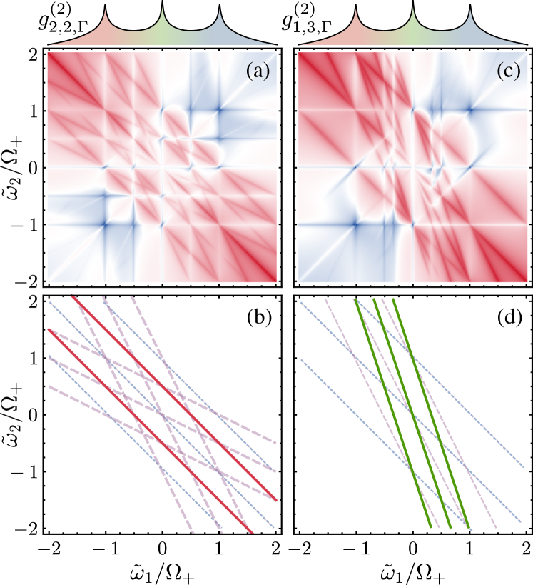
Figure 6: (Color online). Correlation involving four photons. (a) Landscape of correlations between two-photon bundles as given by $g_{2,2,\Gamma}^{(2)}(\omega_{1},\omega_{2})$. (b) Anticorrelations lines due to the transitions $\tilde{\omega}_{1}+\tilde{\omega}_{2}=\Delta$ (shown as dotted blue lines), $\tilde{\omega}_{1}+2\tilde{\omega}_{2}=\Delta$ and $2\tilde{\omega}_{1}+\tilde{\omega}_{2}=\Delta$ (dashed purple), and $2\tilde{\omega}_{1}+2\tilde{\omega}_{2}=\Delta$ (solid red). (c) Correlations between a three-photon bundle, in which each photon has frequency $\tilde{\omega}_{1}$, and a single photon with frequency $\tilde{\omega}_{2}$. (d) Anticorrelations lines due to the transitions $3\tilde{\omega}_{1}+\tilde{\omega}_{2}=\Delta$ (shown in solid green) and the transitions described in (b). The decay rate of the 2LS sets the unit, $\Omega_{+}=300\gamma_{\sigma}$, $\tilde{\omega}_{\sigma}=200\gamma_{\sigma}$ and $\Gamma=5\gamma_{\sigma}$.

The oscillations that are observed in time are characteristic at any order. They are due to the spectral width of the sensors, which detects photon from transitions other than the $N$-photon leapfrog, causing interferences. Such an oscillatory behaviour can be reduced either by turning to a triplet with a larger splitting, in which the emission from different transitions are further apart, or by using a smaller filter width. The photon-bundle correlations however display strikingly the same phenomenology as the photon-photon case of Fig. 4. Namely, they are completely symmetric in time, regardless of the size of the bundle, i.e., the cascade emission of $N$-photon bundles form opposite sides of the Mollow triplet does not have a preferential order. The temporal symmetry can be broken by involving a real transition and when the laser becomes off-resonant to the 2LS. In this way, the Mollow triplet can be turned into a tuneable and versatile source of $N$-photon bundles simply by filtering its emission at the adequate spectral windows.

This physics can be generalized, in principle, to any higher order. Of course, an actual experiment would be increasingly challenged in measuring such correlations. Still, for the sake of illustration, we now quickly address the case of four-photon bundles (and parenthetically the general case of $N$-photon bundles). The leapfrog are then hyperplanes of dimension 3 ($N$) in an hyperspace of dimension 4 ($N+1$), which we shall not attempt to represent. Instead, we show the two-bundle correlation spectra, in Fig. 6. When correlating two bundles of two-photons each, we recover a landscape fairly similar to that of Fig. 1. When correlating a photon with the rest of the bundle, we turn to the heralding scenario. The number of possibilities is that given by the integer partition of 3 ($N$), which is conveniently represented as Young tableaux, whose number of row is the order of the correlation, and with each entry providing the composition of the correlated bundles:

1. (1,1,1,1) for $g^{(4)}_{1,1,1,1}$, the standard Glauber correlator $g^{(4)}$,

2. (2,2) for $g^{(2)}_{2,2}$, shown in Fig. 6(a),

3. (1,3) for $g^{(2)}_{1,3}$, shown in Fig. 6(b),

4. (1,1,2) for $g^{(3)}_{1,1,2}$.

The non-partitioned case (4) does not lead to a correlator (it could be understood as normal luminescence). Maybe the most useful configuration is ${\tiny\yng(1,2)}\cdots{\tiny\yng(2)}$, with a single photon heralding a $N$-photon bundle. The case of one photon heralding a 3-photon bundle lies on any of the corresponding leapfrogs shown as the steepest lines in Fig. 6(b), with equation $N\tilde{\omega}_{1}+\tilde{\omega}_{2}=\Delta$ (the case $N=3$ applies in the figure). While it might be less obvious that other configurations could also be useful, it would not be surprising on the other hand that the need could arise with the boom of quantum technologies. It is clear that, in such a case, the Mollow triplet can serve as a universal photon-emitter, able to deliver any requested configuration, e.g., distributing ten photons in a five channel input with two single photons, two two-photon bundles and a four-photon bundle:

$${\tiny\yng(1,1,2,2,4)}\,.$$ (13)

Would such a profile be required to feed a quantum gate, it is a small technical matter to identify which spectral windows would capture this configuration and filter it out from the total luminescence. Once again, we do not here address specifically the issue of the signal, but only point to the structure of the photon correlations that reside in the Mollow triplet. We highlight as well that, in addition to feeding boson sampling devices, the very combinatorial nature of the emission could allow to test quantum supremacy through photon detection only, without the need of interposing a complex Galton board of optical beam-splitters. Whatever its actual use for practical applications, it is clear that the Mollow triplet overflows with possibilities, so characteristic of strongly-correlated quantum emission.

VII Conclusions and Perspectives

We have shown that the Mollow triplet is a treasure trove of quantum correlations, at all orders and not limited to dressed-state transitions. Specifically, we have shown—based on both qualitative arguments rooted in the structure of the dressed-atom ladder and exact computations made possible by a recent theory of frequency-resolved $N$-photon correlations—that the emission from the Mollow triplet exhibits its richest potential when dealing with leapfrog transitions, i.e., processes that occur through virtual photons, endowing them with much stronger correlations.

While the focus of photon correlations from the Mollow triplet has been on correlations between two photons from the peaks, following the picture of a radiative cascade between dressed states, our results should encourage the study of correlations from photons away from the spectral peaks, where the emission from a Mollow triplet at the appropriate frequencies can be used as a heralded source of $N$-photon bundles or, taking full advantage of the scheme, any customisable configuration of photons. At an applied level, including with the use of cavities to Purcell enhance these transitions and turn the virtual processes into real ones, this should allow to develop new types of quantum emitters, of interest for instance for multiphoton quantum spectroscopy lopezcarreno15a , or to deepen the tests of nonlocality and quantum interferences between correlated photons peiris17a . Our result only scratches the surface of the possibilities that reside in the Mollow triplet, which should be of interest as programmable quantum inputs for future photonic applications.

References

- (1) Vogel, W. & Welsch, D.-G. Quantum Optics (Wiley-VCH, 3, 2006).
- (2) Carmichael, H. J. & Walls, D. F. A quantum-mechanical master equation treatment of the dynamical Stark effect. J. Phys. B.: At. Mol. Phys. 9, 1199 (1976).
- (3) Kimble, H. J., Dagenais, M. & Mandel, L. Photon antibunching in resonance fluorescence. Phys. Rev. Lett. 39, 691 (1977).
- (4) Heitler, W. The Quantum Theory of Radiation (Oxford University Press, 1944).
- (5) López Carreño, J. C., Sánchez Muñoz, C., del Valle, E. & Laussy, F. P. Excitation with quantum light. II. Exciting a two-level system. Phys. Rev. A 94, 063826 (2016).
- (6) Aharonovich, I., Englund, D. & Toth, M. Solid-state single-photon emitters. Nat. Photon. 10, 631 (2016).
- (7) Mollow, B. R. Power spectrum of light scattered by two-level systems. Phys. Rev. 188, 1969 (1969).
- (8) Schuda, F., Jr, C. R. S. & Hercher, M. Observation of the resonant Stark effect at optical frequencies. J. Phys. B.: At. Mol. Phys. 7, L198 (1974).
- (9) Keitel, C. H., Knight, P. L., Narducci, L. M. & Scully, M. O. Resonance fluorescence in a tailored vacuum. Opt. Commun. 118, 143 (1995).
- (10) Bienert, M., Merkel, W. & Morigi, G. Resonance fluorescence of a trapped three-level atom. Phys. Rev. A 69, 013405 (2004).
- (11) Bienert, M., Torres, J. M., Zippilli, S. & Morigi, G. Resonance fluorescence of a cold atom in a high-finesse resonator. Phys. Rev. A 76, 013410 (2007).
- (12) Flagg, E. B. et al. Resonantly driven coherent oscillations in a solid-state quantum emitter. Nat. Phys. 5, 203 (2009).
- (13) Astafiev, O. et al. Resonance fluorescence of a single artificial atom. Science 327, 840 (2010).
- (14) Makhonin, M. N. et al. Waveguide coupled resonance fluorescence from on-chip quantum emitter. Nano Lett. 14, 6997 (2014).
- (15) Toyli, D. M. et al. Resonance fluorescence from an artificial atom in squeezed vacuum. Phys. Rev. X 6, 031004 (2016).
- (16) Unsleber, S. et al. Highly indistinguishable on-demand resonance fluorescence photons from a deterministic quantum dot micropillar device with 74% extraction efficiency. Opt. Express 24, 8539 (2016).
- (17) Lagoudakis, K. et al. Observation of mollow triplets with tunable interactions in double lambda systems of individual hole spins. Phys. Rev. Lett. 118, 013602 (2017).
- (18) Cohen-Tannoudji, C. N. & Reynaud, S. Dressed-atom description of resonance fluorescence and absorption spectra of a multi-level atom in an intense laser beam. J. Phys. B.: At. Mol. Phys. 10, 345 (1977).
- (19) Reynaud, S. La fluorescence de résonance: étude par la méthode de l’atome habillé. Annales de Physique 8, 315 (1983).
- (20) Apanasevich, P. A. & Kilin, S. Y. Photon bunching and antibunching in resonance fluorescence. J. Phys. B.: At. Mol. Phys. 12, L83 (1979).
- (21) Cohen-Tannoudji, C. & Reynaud, S. Atoms in strong light-fields: Photon antibunching in single atom fluorescence. Phil. Trans. R. Soc. Lond. A 293, 223 (1979).
- (22) Aspect, A., Roger, G., Reynaud, S., Dalibard, J. & Cohen-Tannoudji, C. Time correlations between the two sidebands of the resonance fluorescence triplet. Phys. Rev. Lett. 45, 617 (1980).
- (23) Al-Hilfy, A. & Loudon, R. Theory of photon correlations in two-photon cascade emission. J. Phys. B.: At. Mol. Phys. 18, 3697 (1985).
- (24) Schrama, C. A., Nienhuis, G., Dijkerman, H. A., Steijsiger, C. & Heideman, H. G. M. Destructive interference between opposite time orders of photon emission. Phys. Rev. Lett. 67 (1991).
- (25) Schrama, C. A., Nienhuis, G., Dijkerman, H. A., Steijsiger, C. & Heideman, H. G. M. Intensity correlations between the components of the resonance fluorescence triplet. Phys. Rev. A 45, 8045 (1992).
- (26) Ulhaq, A. et al. Cascaded single-photon emission from the Mollow triplet sidebands of a quantum dot. Nat. Photon. 6, 238 (2012).
- (27) Arnoldus, H. F. & Nienhuis, G. Photon correlations between the lines in the spectrum of resonance fluorescence. J. Phys. B.: At. Mol. Phys. 17, 963 (1984).
- (28) Knöll, L., Weber, G. & Schafer, T. Theory of time-resolved correlation spectroscopy and its application to resonance fluorescence radiation. J. Phys. B.: At. Mol. Phys. 17, 4861 (1984).
- (29) Nienhuis, G. Spectral correlations in resonance fluorescence. Phys. Rev. A 47, 510 (1993).
- (30) Knöll, L. & Weber, G. Theory of -fold time-resolved correlation spectroscopy and its application to resonance fluorescence radiation. J. Phys. B.: At. Mol. Phys. 19, 2817 (1986).
- (31) del Valle, E., González-Tudela, A., Laussy, F. P., Tejedor, C. & Hartmann, M. J. Theory of frequency-filtered and time-resolved -photon correlations. Phys. Rev. Lett. 109, 183601 (2012).
- (32) González-Tudela, A., Laussy, F. P., Tejedor, C., Hartmann, M. J. & del Valle, E. Two-photon spectra of quantum emitters. New J. Phys. 15, 033036 (2013).
- (33) del Valle, E. Distilling one, two and entangled pairs of photons from a quantum dot with cavity QED effects and spectral filtering. New J. Phys. 15, 025019 (2013).
- (34) Sánchez Muñoz, C., del Valle, E., Tejedor, C. & Laussy, F. Violation of classical inequalities by photon frequency filtering. Phys. Rev. A 90, 052111 (2014).
- (35) Peiris, M. et al. Two-color photon correlations of the light scattered by a quantum dot. Phys. Rev. B 91, 195125 (2015).
- (36) del Valle, E., González-Tudela, A., Cancellieri, E., Laussy, F. P. & Tejedor, C. Generation of a two-photon state from a quantum dot in a microcavity. New J. Phys. 13, 113014 (2011).
- (37) González-Tudela, A., del Valle, E. & Laussy, F. P. Optimization of photon correlations by frequency filtering. Phys. Rev. A 91, 043807 (2015).
- (38) Peiris, M., Konthasinghe, K. & Muller, A. Franson interference generated by a two-level system. Phys. Rev. Lett. 118, 030501 (2017).
- (39) Glauber, R. J. Photon correlations. Phys. Rev. Lett. 10, 84 (1963).
- (40) Sánchez Muñoz, C. et al. Emitters of -photon bundles. Nat. Photon. 8, 550 (2014).
- (41) Sánchez Muñoz, C., Laussy, F. P., Tejedor, C. & del Valle, E. Enhanced two-photon emission from a dressed biexciton. New J. Phys. 17, 123021 (2015).
- (42) López Carreño, J. C., Sánchez Muñoz, C., Sanvitto, D., del Valle, E. & Laussy, F. P. Exciting polaritons with quantum light. Phys. Rev. Lett. 115, 196402 (2015).