An efficient spectral-Galerkin approximation and error analysis for Maxwell transmission eigenvalue problems in spherical geometries thanks: This work was supported in part by the National Natural Science Foundation of China (No. 11661022, 11471031, 91430216), NASF U1530401, and the US National Science Foundation grant DMS-1419040.

Jing An Beijing Computational Science Research Center, Beijing 100193, China (anjing@csrc.ac.cn); and School of Mathematical Sciences, Guizhou Normal University, Guiyang 550025, China (aj154@163.com).    Zhimin Zhang Beijing Computational Science Research Center, Beijing 100193, China (zmzhang@csrc.ac.cn); and Department of Mathematics, Wayne State University, Detroit, MI 48202, USA (zzhang@math.wayne.edu).
Abstract

We propose and analyze an efficient spectral-Galerkin approximation for the Maxwell transmission eigenvalue problem in spherical geometry. Using a vector spherical harmonic expansion, we reduce the problem to a sequence of equivalent one-dimensional TE and TM modes that can be solved individually in parallel. For the TE mode, we derive associated generalized eigenvalue problems and corresponding pole conditions. Then we introduce weighted Sobolev spaces based on the pole condition and prove error estimates for the generalized eigenvalue problem. The TM mode is a coupled system with four unknown functions, which is challenging for numerical calculation. To handle it, we design an effective algorithm using Legendre-type vector basis functions. Finally, we provide some numerical experiments to validate our theoretical results and demonstrate the efficiency of the algorithms.

Keywords: Maxwell transmission eigenvalue problems, spherical geometry, TE and TM modes, spectral-Galerkin approximation, error analysis

1 Introduction

The Maxwell transmission eigenvalue problem is a boundary value problem in a bounded domain which arises in inverse scattering theory for inhomogeneous media. It is well known that the transmission eigenvalues play a critical role in the reconstruction of inhomogeneous non-absorbing media [1, 2, 3]. In addition, the transmission eigenvalues are also used to estimate the index of refraction of a non-absorbing inhomogeneous medium in recent years[4, 5, 6]. The method consists of several steps. First of all, the support of the scattering obstacle can be recovered by using the measured scattering data and the linear sampling method [7] and the transmission eigenvalues can be identified from either the far field or near field data [8, 4]. Then, the bounds for smallest and largest eigenvalues of the (matrix) index of refraction can be obtained in terms of the support of the scattering obstacle and the first transmission eigenvalue of the anisotropic media [9]. Finally, reconstructions of the electric permittivity (if it is a scalar constant) or an estimate of the eigenvalues of the matrix in the case of anisotropic permittivity can be obtained [7].

However, the effectiveness of the above method rests on having an efficient and robust algorithm for computing Maxwell transmission eigenvalues. Although the Maxwell transmission eigenvalue problem is stated in a simple form, its solution is complex since it is nonstandard so that the classical theory can not be applied directly. There are only a few papers dealing with the numerical computation of Maxwell transmission eigenvalues due to this notorious difficulty. In [10], Monk et al. propose two finite element methods in computing a few lowest Maxwell’s transmission eigenvalues, curl-conforming finite element and mixed finite element methods. In [3], Sun et al. presented an iterative method to compute the Maxwell’s transmission eigenvalue, where the transmission eigenvalue problem is written as a quad-curl eigenvalue problem. Then the real transmission eigenvalues are shown to be the roots of a nonlinear function whose value is the generalized eigenvalue of a related self-adjoint quad-curl eigenvalue problem which is computed by using a mixed finite element method. In [11], Huang et al. also proposed a numerical algorithm for computing Maxwell transmission eigenvalue problems. However, all these methods are based on low-order finite element methods, so they become very expensive if high accuracy is needed. To the best of our knowledge, no error analysis is given yet for any existing numerical method, even for three-dimensional spherical domains.

In practical applications, we often need to solve Maxwell transmission eigenvalue problems on the special domain of spherical geometries. We know of only a few reports on spectral-Galerkin approximation for the Maxwell transmission eigenvalue problems on the special domain of spherical geometries. Thus, we will present in this paper an efficient spectral-Galerkin approximation for the Maxwell transmission eigenvalue problem in spherical geometry. Using a vector spherical harmonic expansion, we reduce the problem to a sequence of equivalent one-dimensional TE and TM modes that can be solved individually in parallel. For the TE mode, we derive associated generalized eigenvalue problems and corresponding pole conditions. Then we introduce weighted Sobolev spaces corresponding to the pole condition and prove error estimates for the generalized eigenvalue problem. The TM mode is a coupled system with four unknown functions, which is challenging for numerical calculation. To handle it, we design an effective algorithm using Legendre-type vector basis functions. Finally, we provide some numerical experiments to validate our theoretical results and demonstrate the efficiency of the algorithms.

The rest of this paper is organized as follows. In the next section, we introduce the Maxwell transmission eigenvalue problem. In §3, we derive a dimension reduction scheme under spherical geometries. In §4, we derive the weak formulation and error estimate for the TE mode. In §5, we describe in detail an efficient implementation of the algorithm. We present several numerical experiments in §6 to demonstrate the accuracy and efficiency of our method. Finally, in §7 we give some concluding remarks.

2 Maxwell transmission eigenvalue problem

Let D3𝐷superscript3D\subset\mathbb{R}^{3} be a bounded simply connected region with piecewise smooth boundary D𝐷\partial D and denote by 𝝂𝝂\boldsymbol{\nu} the outward normal vector to D𝐷\partial D. Let (.,.)D(.,.)_{D} denote the scalar product in L2(D)3superscript𝐿2superscript𝐷3L^{2}(D)^{3} and define the Hilbert spaces

H(𝐜𝐮𝐫𝐥,D):={𝐮L2(D)3:𝐜𝐮𝐫𝐥𝐮L2(D)3},assign𝐻𝐜𝐮𝐫𝐥𝐷conditional-set𝐮superscript𝐿2superscript𝐷3𝐜𝐮𝐫𝐥𝐮superscript𝐿2superscript𝐷3\displaystyle H(\mathbf{curl},D):=\{\mathbf{u}\in{L^{2}(D)}^{3}:\mathbf{curl}\;\mathbf{u}\in L^{2}(D)^{3}\},
H0(𝐜𝐮𝐫𝐥,D):={𝐮H(𝐜𝐮𝐫𝐥,D):𝐮×𝝂=𝟎onD}assignsubscript𝐻0𝐜𝐮𝐫𝐥𝐷conditional-set𝐮𝐻𝐜𝐮𝐫𝐥𝐷𝐮𝝂0on𝐷\displaystyle H_{0}(\mathbf{curl},D):=\{\mathbf{u}\in H(\mathbf{curl},D):\mathbf{u}\times\boldsymbol{\nu}=\boldsymbol{0}~{}\text{on}~{}\partial D\}

equipped with the scalar product (𝐮,𝐯)𝐜𝐮𝐫𝐥=(𝐮,𝐯)D+(𝐜𝐮𝐫𝐥𝐮,𝐜𝐮𝐫𝐥𝐯)Dsubscript𝐮𝐯𝐜𝐮𝐫𝐥subscript𝐮𝐯𝐷subscript𝐜𝐮𝐫𝐥𝐮𝐜𝐮𝐫𝐥𝐯𝐷(\mathbf{u},\mathbf{v})_{\mathbf{curl}}=(\mathbf{u},\mathbf{v})_{D}+(\mathbf{curl}\;\mathbf{u},\mathbf{curl}\;\mathbf{v})_{D} and the corresponding norm 𝐜𝐮𝐫𝐥\|\cdot\|_{\mathbf{curl}}. Following [12], we also define

𝒰(D):={𝐮H(𝐜𝐮𝐫𝐥,D):𝐜𝐮𝐫𝐥𝐮H(𝐜𝐮𝐫𝐥,D)},assign𝒰𝐷conditional-set𝐮𝐻𝐜𝐮𝐫𝐥𝐷𝐜𝐮𝐫𝐥𝐮𝐻𝐜𝐮𝐫𝐥𝐷\displaystyle\mathcal{U}(D):=\{\mathbf{u}\in H(\mathbf{curl},D):\mathbf{curl}\;\mathbf{u}\in H(\mathbf{curl},D)\},
𝒰0(D):={𝐮H0(𝐜𝐮𝐫𝐥,D):𝐜𝐮𝐫𝐥𝐮H0(𝐜𝐮𝐫𝐥,D)}assignsubscript𝒰0𝐷conditional-set𝐮subscript𝐻0𝐜𝐮𝐫𝐥𝐷𝐜𝐮𝐫𝐥𝐮subscript𝐻0𝐜𝐮𝐫𝐥𝐷\displaystyle\mathcal{U}_{0}(D):=\{\mathbf{u}\in H_{0}(\mathbf{curl},D):\mathbf{curl}\;\mathbf{u}\in H_{0}(\mathbf{curl},D)\}

equipped with the scalar product (𝐮,𝐯)𝒰=(𝐮,𝐯)𝐜𝐮𝐫𝐥+(𝐜𝐮𝐫𝐥𝐮,𝐜𝐮𝐫𝐥𝐯)𝐜𝐮𝐫𝐥subscript𝐮𝐯𝒰subscript𝐮𝐯𝐜𝐮𝐫𝐥subscript𝐜𝐮𝐫𝐥𝐮𝐜𝐮𝐫𝐥𝐯𝐜𝐮𝐫𝐥(\mathbf{u},\mathbf{v})_{\mathcal{U}}=(\mathbf{u},\mathbf{v})_{\mathbf{curl}}+(\mathbf{curl}\;\mathbf{u},\mathbf{curl}\;\mathbf{v})_{\mathbf{curl}} and the corresponding norm 𝒰\|\cdot\|_{\mathcal{U}}.

Let 𝑵𝑵\boldsymbol{N} be a 3×3333\times 3 matrix valued function defined on D𝐷D such that 𝑵L(D,3×3)𝑵superscript𝐿𝐷superscript33\boldsymbol{N}\in L^{\infty}(D,\mathbb{R}^{3\times 3}). Definition 2.1 A real matrix field 𝑵𝑵\boldsymbol{N} is said to be bounded positive definite on D𝐷D if 𝑵L(D,3×3)𝑵superscript𝐿𝐷superscript33\boldsymbol{N}\in L^{\infty}(D,\mathbb{R}^{3\times 3}) and there exists a constant γ>0𝛾0\gamma>0 such that

ξ¯𝑵ξγ|ξ|2,ξ3 a.e in D.formulae-sequence¯𝜉𝑵𝜉𝛾superscript𝜉2for-all𝜉superscript3 a.e in 𝐷\displaystyle\bar{\mathbf{\xi}}\cdot\boldsymbol{N}\mathbf{\xi}\geq\gamma|\mathbf{\xi}|^{2},\forall\mathbf{\xi}\in\mathbb{C}^{3}\text{~{}~{}a.e in }D.

We further assume that 𝑵,𝑵1𝑵superscript𝑵1\boldsymbol{N},\boldsymbol{N}^{-1} and (𝑵𝑰)1superscript𝑵𝑰1(\boldsymbol{N}-\boldsymbol{I})^{-1} or (𝑰𝑵)1superscript𝑰𝑵1(\boldsymbol{I}-\boldsymbol{N})^{-1} are bounded positive definite real matrix fields on D𝐷D. The interior transmission eigenvalue problem for the anisotropic Maxwell’s equations in terms of electric fields is formulated as the problem of finding two vector valued functions 𝐄L2(D)3𝐄superscript𝐿2superscript𝐷3\mathbf{E}\in{L^{2}(D)}^{3} and 𝐄𝟎L2(D)3subscript𝐄0superscript𝐿2superscript𝐷3\mathbf{E_{0}}\in{L^{2}(D)}^{3} such that 𝐄𝐄𝟎𝒰0(D)𝐄subscript𝐄0subscript𝒰0𝐷\mathbf{E}-\mathbf{E_{0}}\in\mathcal{U}_{0}(D) satisfies [3, 10]:

𝐜𝐮𝐫𝐥𝐜𝐮𝐫𝐥𝐄k2𝑵𝐄=0𝐜𝐮𝐫𝐥𝐜𝐮𝐫𝐥𝐄superscript𝑘2𝑵𝐄0\displaystyle\mathbf{curl}\mathbf{curl}\mathbf{E}-k^{2}\boldsymbol{N}\mathbf{E}=0 inD,in𝐷\displaystyle~{}~{}~{}~{}~{}~{}~{}\text{in}~{}~{}~{}D, (2.1)
𝐜𝐮𝐫𝐥𝐜𝐮𝐫𝐥𝐄𝟎k2𝐄𝟎=0subscript𝐜𝐮𝐫𝐥𝐜𝐮𝐫𝐥𝐄0superscript𝑘2subscript𝐄00\displaystyle\mathbf{curl}\mathbf{curl}\mathbf{E_{0}}-k^{2}\mathbf{E_{0}}=0 inD,in𝐷\displaystyle~{}~{}~{}~{}~{}~{}~{}\text{in}~{}~{}~{}D, (2.2)
𝐄×𝝂=𝐄0×𝝂𝐄𝝂subscript𝐄0𝝂\displaystyle\mathbf{E}\times\boldsymbol{\nu}=\mathbf{E}_{0}\times\boldsymbol{\nu} onD,on𝐷\displaystyle~{}~{}~{}~{}~{}~{}~{}\text{on}~{}~{}~{}\partial D, (2.3)
𝐜𝐮𝐫𝐥𝐄×𝝂=𝐜𝐮𝐫𝐥𝐄0×𝝂𝐜𝐮𝐫𝐥𝐄𝝂subscript𝐜𝐮𝐫𝐥𝐄0𝝂\displaystyle\mathbf{curl}\mathbf{E}\times\boldsymbol{\nu}=\mathbf{curl}\mathbf{E}_{0}\times\boldsymbol{\nu} onD.on𝐷\displaystyle~{}~{}~{}~{}~{}~{}~{}\text{on}~{}~{}~{}\partial D. (2.4)

3 Dimension reduction scheme under spherical geometries

We shall restrict our attention to the case where D𝐷D is a ball of radius R𝑅R and 𝑵=n𝑰𝑵𝑛𝑰\boldsymbol{N}=n\boldsymbol{I} with n𝑛n being a function along the radial direction. In this case, by using vector spherical harmonic expansion we can reduce the problem to a sequence of equivalent one-dimensional TE and TM modes that can be solved individually in parallel.

3.1 Vector spherical harmonics

There are several versions with different notation and properties for vector spherical harmonics (see e.g.,[13, 14, 15, 16]). We adopt in this paper the family of vector spherical harmonics in [13, 14].

The spherical coordinates (r,θ,ϕ)𝑟𝜃italic-ϕ(r,\theta,\phi) are related to the Cartesian coordinates 𝐱=(x1,x2,x3)𝐱subscript𝑥1subscript𝑥2subscript𝑥3\mathbf{x}=(x_{1},x_{2},x_{3}) by

x1=rsinθcosϕ,x2=rsinθsinϕ,x3=rcosθ.formulae-sequencesubscript𝑥1𝑟𝜃italic-ϕformulae-sequencesubscript𝑥2𝑟𝜃italic-ϕsubscript𝑥3𝑟𝜃\displaystyle x_{1}=r\sin\theta\cos\phi,\quad x_{2}=r\sin\theta\sin\phi,\quad x_{3}=r\cos\theta. (3.1)

Let

𝐞r=𝐱r,𝐞θ=(sinθcosϕ,sinθsinϕ,sinθ),𝐞ϕ=(sinϕ,cosϕ,0).formulae-sequencesubscript𝐞𝑟𝐱𝑟formulae-sequencesubscript𝐞𝜃𝜃italic-ϕ𝜃italic-ϕ𝜃subscript𝐞italic-ϕitalic-ϕitalic-ϕ0\displaystyle\mathbf{e}_{r}=\frac{\mathbf{x}}{r},\quad\mathbf{e}_{\theta}=(\sin\theta\cos\phi,\sin\theta\sin\phi,-\sin\theta),\quad\mathbf{e}_{\phi}=(-\sin\phi,\cos\phi,0). (3.2)

Then {𝐞r,𝐞θ,𝐞ϕ}subscript𝐞𝑟subscript𝐞𝜃subscript𝐞italic-ϕ\{\mathbf{e}_{r},\mathbf{e}_{\theta},\mathbf{e}_{\phi}\} forms a moving orthonormal coordinate basis in 3superscript3\mathbb{R}^{3}.

Let S𝑆S be the unit spherical surface, and denote by ΔSsubscriptΔ𝑆\Delta_{S} and Ssubscript𝑆\nabla_{S} the Laplace-Beltrami and tangential gradient operators on S𝑆S, namely,

Su=1sinθθ(sinθuθ)+1sin2θ2uϕ2,subscript𝑆𝑢1𝜃𝜃𝜃𝑢𝜃1superscript2𝜃superscript2𝑢superscriptitalic-ϕ2\displaystyle\triangle_{S}u=\frac{1}{\sin\theta}\frac{\partial}{\partial\theta}(\sin\theta\frac{\partial u}{\partial\theta})+\frac{1}{\sin^{2}\theta}\frac{\partial^{2}u}{\partial\phi^{2}}, (3.3)
Su=uθ𝐞θ+1sinθuϕ𝐞ϕ.subscript𝑆𝑢𝑢𝜃subscript𝐞𝜃1𝜃𝑢italic-ϕsubscript𝐞italic-ϕ\displaystyle\nabla_{S}u=\frac{\partial u}{\partial\theta}\mathbf{e}_{\theta}+\frac{1}{\sin\theta}\frac{\partial u}{\partial\phi}\mathbf{e}_{\phi}. (3.4)

The spherical harmonics {Ylm}superscriptsubscript𝑌𝑙𝑚\{Y_{l}^{m}\} (as normalized in [13]) are eigenfunctions of ΔSsubscriptΔ𝑆\Delta_{S}, i.e.,

ΔSYlm=l(l+1)Ylm,l0,|m|l;formulae-sequencesubscriptΔ𝑆superscriptsubscript𝑌𝑙𝑚𝑙𝑙1superscriptsubscript𝑌𝑙𝑚formulae-sequence𝑙0𝑚𝑙\displaystyle\Delta_{S}Y_{l}^{m}=-l(l+1)Y_{l}^{m},\quad l\geq 0,\;|m|\leq l; (3.5)

and form an orthonormal basis for L2(S)superscript𝐿2𝑆L^{2}(S):

SYlmYlm𝑑S=δllδmm.subscript𝑆superscriptsubscript𝑌𝑙𝑚superscriptsubscript𝑌superscript𝑙superscript𝑚differential-d𝑆subscript𝛿𝑙superscript𝑙subscript𝛿𝑚superscript𝑚\displaystyle\int_{S}Y_{l}^{m}Y_{l^{\prime}}^{m^{\prime}}dS=\delta_{ll^{\prime}}\delta_{mm^{\prime}}. (3.6)

The family of vector spherical harmonics is defined by [13]:

𝐓lm=SYlm×𝐞r=1sinθYlmϕ𝐞θYlmθ𝐞ϕ,superscriptsubscript𝐓𝑙𝑚subscript𝑆superscriptsubscript𝑌𝑙𝑚subscript𝐞𝑟1𝜃superscriptsubscript𝑌𝑙𝑚italic-ϕsubscript𝐞𝜃superscriptsubscript𝑌𝑙𝑚𝜃subscript𝐞italic-ϕ\displaystyle\mathbf{T}_{l}^{m}=\nabla_{S}Y_{l}^{m}\times\mathbf{e}_{r}=\frac{1}{\sin\theta}\frac{\partial Y_{l}^{m}}{\partial\phi}\mathbf{e}_{\theta}-\frac{\partial Y_{l}^{m}}{\partial\theta}\mathbf{e}_{\phi}, forl1,0|m|l,formulae-sequencefor𝑙10𝑚𝑙\displaystyle\text{for}~{}~{}l\geq 1,0\leq|m|\leq l, (3.7)
𝐕lm=(l+1)Ylm𝐞rSYlm,superscriptsubscript𝐕𝑙𝑚𝑙1superscriptsubscript𝑌𝑙𝑚subscript𝐞𝑟subscript𝑆superscriptsubscript𝑌𝑙𝑚\displaystyle\mathbf{V}_{l}^{m}=(l+1)Y_{l}^{m}\mathbf{e}_{r}-\nabla_{S}Y_{l}^{m}, forl0,0|m|l,formulae-sequencefor𝑙00𝑚𝑙\displaystyle\text{for}~{}~{}l\geq 0,0\leq|m|\leq l, (3.8)
𝐖lm=lYlm𝐞r+SYlm,superscriptsubscript𝐖𝑙𝑚𝑙superscriptsubscript𝑌𝑙𝑚subscript𝐞𝑟subscript𝑆superscriptsubscript𝑌𝑙𝑚\displaystyle\mathbf{W}_{l}^{m}=lY_{l}^{m}\mathbf{e}_{r}+\nabla_{S}Y_{l}^{m}, forl1,0|m|l,formulae-sequencefor𝑙10𝑚𝑙\displaystyle\text{for}~{}~{}l\geq 1,0\leq|m|\leq l, (3.9)

where 𝐕00=14π𝐞rsuperscriptsubscript𝐕0014𝜋subscript𝐞𝑟\mathbf{V}_{0}^{0}=\frac{1}{\sqrt{4\pi}}\mathbf{e}_{r}. With the understanding of 𝐓00=𝐖00=𝟎,superscriptsubscript𝐓00superscriptsubscript𝐖000\mathbf{T}_{0}^{0}=\mathbf{W}_{0}^{0}=\mathbf{0}, the indexes {l,m}𝑙𝑚\{l,m\} run over {(l,m):l0,0|m|l}.conditional-set𝑙𝑚formulae-sequence𝑙00𝑚𝑙\{(l,m):l\geq 0,0\leq|m|\leq l\}.

The following lemma was proved in [13] ((A.1)𝐴.1(A.1) and (A.2)𝐴.2(A.2))
Lemma 3.1

S𝐓lm𝐕lm¯𝑑S=S𝐓lm𝐖lm¯𝑑S=S𝐕lm𝐖lm¯𝑑S=0,subscript𝑆superscriptsubscript𝐓𝑙𝑚¯superscriptsubscript𝐕superscript𝑙superscript𝑚differential-d𝑆subscript𝑆superscriptsubscript𝐓𝑙𝑚¯superscriptsubscript𝐖superscript𝑙superscript𝑚differential-d𝑆subscript𝑆superscriptsubscript𝐕𝑙𝑚¯superscriptsubscript𝐖superscript𝑙superscript𝑚differential-d𝑆0\displaystyle\int_{S}\mathbf{T}_{l}^{m}\cdot\overline{\mathbf{V}_{l^{\prime}}^{m^{\prime}}}dS=\int_{S}\mathbf{T}_{l}^{m}\cdot\overline{\mathbf{W}_{l^{\prime}}^{m^{\prime}}}dS=\int_{S}\mathbf{V}_{l}^{m}\cdot\overline{\mathbf{W}_{l^{\prime}}^{m^{\prime}}}dS=0, (3.10)
S𝐕lm𝐕lm¯𝑑S=(l+1)(2l+1)δllδmm,S𝐓lm𝐓lm¯𝑑S=l(l+1)δllδmm,formulae-sequencesubscript𝑆superscriptsubscript𝐕𝑙𝑚¯superscriptsubscript𝐕superscript𝑙superscript𝑚differential-d𝑆𝑙12𝑙1subscript𝛿𝑙superscript𝑙subscript𝛿𝑚superscript𝑚subscript𝑆superscriptsubscript𝐓𝑙𝑚¯superscriptsubscript𝐓superscript𝑙superscript𝑚differential-d𝑆𝑙𝑙1subscript𝛿𝑙superscript𝑙subscript𝛿𝑚superscript𝑚\displaystyle\int_{S}\mathbf{V}_{l}^{m}\cdot\overline{\mathbf{V}_{l^{\prime}}^{m^{\prime}}}dS=(l+1)(2l+1)\delta_{ll^{\prime}}\delta_{mm^{\prime}},\int_{S}\mathbf{T}_{l}^{m}\cdot\overline{\mathbf{T}_{l^{\prime}}^{m^{\prime}}}dS=l(l+1)\delta_{ll^{\prime}}\delta_{mm^{\prime}}, (3.11)
S𝐖lm𝐖lm¯𝑑S=l(2l+1)δllδmm,S𝐓lmSYlmdS=0,formulae-sequencesubscript𝑆superscriptsubscript𝐖𝑙𝑚¯superscriptsubscript𝐖superscript𝑙superscript𝑚differential-d𝑆𝑙2𝑙1subscript𝛿𝑙superscript𝑙subscript𝛿𝑚superscript𝑚subscript𝑆superscriptsubscript𝐓𝑙𝑚subscript𝑆superscriptsubscript𝑌𝑙𝑚𝑑𝑆0\displaystyle\int_{S}\mathbf{W}_{l}^{m}\cdot\overline{\mathbf{W}_{l^{\prime}}^{m^{\prime}}}dS=l(2l+1)\delta_{ll^{\prime}}\delta_{mm^{\prime}},\int_{S}\mathbf{T}_{l}^{m}\cdot\nabla_{S}Y_{l}^{m}dS=0, (3.12)
SSYlmSYlmdS=l(l+1)δllδmm.subscript𝑆subscript𝑆superscriptsubscript𝑌𝑙𝑚subscript𝑆superscriptsubscript𝑌superscript𝑙superscript𝑚𝑑𝑆𝑙𝑙1subscript𝛿𝑙superscript𝑙subscript𝛿𝑚superscript𝑚\displaystyle\int_{S}\nabla_{S}Y_{l}^{m}\cdot\nabla_{S}Y_{l^{\prime}}^{m^{\prime}}dS=l(l+1)\delta_{ll^{\prime}}\delta_{mm^{\prime}}. (3.13)

Let f𝑓f is a function along the radial direction and define the differentiation operators:

dl+=ddr+lr,dl=ddrlr.formulae-sequencesuperscriptsubscript𝑑𝑙𝑑𝑑𝑟𝑙𝑟superscriptsubscript𝑑𝑙𝑑𝑑𝑟𝑙𝑟\displaystyle d_{l}^{+}=\frac{d}{dr}+\frac{l}{r},\quad d_{l}^{-}=\frac{d}{dr}-\frac{l}{r}. (3.14)

The following lemma is again proved in [13] ((A.9)𝐴.9(A.9)):
Lemma 3.2

𝐜𝐮𝐫𝐥(f𝐕lm)=(dl+2+f)𝐓lm,𝐜𝐮𝐫𝐥(f𝐖lm)=(dl1f)𝐓lm,formulae-sequence𝐜𝐮𝐫𝐥𝑓superscriptsubscript𝐕𝑙𝑚superscriptsubscript𝑑𝑙2𝑓superscriptsubscript𝐓𝑙𝑚𝐜𝐮𝐫𝐥𝑓superscriptsubscript𝐖𝑙𝑚superscriptsubscript𝑑𝑙1𝑓superscriptsubscript𝐓𝑙𝑚\displaystyle\mathbf{curl}(f\mathbf{V}_{l}^{m})=(d_{l+2}^{+}f)\mathbf{T}_{l}^{m},\quad\mathbf{curl}(f\mathbf{W}_{l}^{m})=-(d_{l-1}^{-}f)\mathbf{T}_{l}^{m}, (3.15)
(2l+1)𝐜𝐮𝐫𝐥(f𝐓lm)=(l+1)(dl+1+f)𝐖lml(dlf)𝐕lm.2𝑙1𝐜𝐮𝐫𝐥𝑓superscriptsubscript𝐓𝑙𝑚𝑙1superscriptsubscript𝑑𝑙1𝑓superscriptsubscript𝐖𝑙𝑚𝑙superscriptsubscript𝑑𝑙𝑓superscriptsubscript𝐕𝑙𝑚\displaystyle(2l+1)\mathbf{curl}(f\mathbf{T}_{l}^{m})=(l+1)(d_{l+1}^{+}f)\mathbf{W}_{l}^{m}-l(d_{l}^{-}f)\mathbf{V}_{l}^{m}. (3.16)

3.2 Dimension reduction scheme

Let us write

𝐄=l=0|m|=0l(vlm(r)𝐕lm(θ,ϕ)+tlm(r)𝐓lm(θ,ϕ)+wlm(r)𝐖lm(θ,ϕ)),𝐄superscriptsubscript𝑙0superscriptsubscript𝑚0𝑙superscriptsubscript𝑣𝑙𝑚𝑟superscriptsubscript𝐕𝑙𝑚𝜃italic-ϕsuperscriptsubscript𝑡𝑙𝑚𝑟superscriptsubscript𝐓𝑙𝑚𝜃italic-ϕsuperscriptsubscript𝑤𝑙𝑚𝑟superscriptsubscript𝐖𝑙𝑚𝜃italic-ϕ\displaystyle\mathbf{E}=\sum_{l=0}^{\infty}\sum_{|m|=0}^{l}(v_{l}^{m}(r)\mathbf{V}_{l}^{m}(\theta,\phi)+t_{l}^{m}(r)\mathbf{T}_{l}^{m}(\theta,\phi)+w_{l}^{m}(r)\mathbf{W}_{l}^{m}(\theta,\phi)), (3.17)
𝐄0=l=0|m|=0l(v¯lm(r)𝐕lm(θ,ϕ)+t¯lm(r)𝐓lm(θ,ϕ)+w¯lm(r)𝐖lm(θ,ϕ)).subscript𝐄0superscriptsubscript𝑙0superscriptsubscript𝑚0𝑙superscriptsubscript¯𝑣𝑙𝑚𝑟superscriptsubscript𝐕𝑙𝑚𝜃italic-ϕsuperscriptsubscript¯𝑡𝑙𝑚𝑟superscriptsubscript𝐓𝑙𝑚𝜃italic-ϕsuperscriptsubscript¯𝑤𝑙𝑚𝑟superscriptsubscript𝐖𝑙𝑚𝜃italic-ϕ\displaystyle\mathbf{E}_{0}=\sum_{l=0}^{\infty}\sum_{|m|=0}^{l}(\bar{v}_{l}^{m}(r)\mathbf{V}_{l}^{m}(\theta,\phi)+\bar{t}_{l}^{m}(r)\mathbf{T}_{l}^{m}(\theta,\phi)+\bar{w}_{l}^{m}(r)\mathbf{W}_{l}^{m}(\theta,\phi)). (3.18)

From Lemma 3.2 we can derive that

𝐜𝐮𝐫𝐥𝐜𝐮𝐫𝐥(vlm(r)𝐕lm(θ,ϕ))=𝐜𝐮𝐫𝐥((dl+2+vlm(r))𝐓lm(θ,ϕ))𝐜𝐮𝐫𝐥𝐜𝐮𝐫𝐥superscriptsubscript𝑣𝑙𝑚𝑟superscriptsubscript𝐕𝑙𝑚𝜃italic-ϕ𝐜𝐮𝐫𝐥superscriptsubscript𝑑𝑙2superscriptsubscript𝑣𝑙𝑚𝑟superscriptsubscript𝐓𝑙𝑚𝜃italic-ϕ\displaystyle\mathbf{curl}\mathbf{curl}(v_{l}^{m}(r)\mathbf{V}_{l}^{m}(\theta,\phi))=\mathbf{curl}((d_{l+2}^{+}v_{l}^{m}(r))\mathbf{T}_{l}^{m}(\theta,\phi))
=l+12l+1(dl+1+dl+2+vlm(r))𝐖lm(θ,ϕ)l2l+1(dldl+2+vlm(r))𝐕lm(θ,ϕ),absent𝑙12𝑙1superscriptsubscript𝑑𝑙1superscriptsubscript𝑑𝑙2superscriptsubscript𝑣𝑙𝑚𝑟superscriptsubscript𝐖𝑙𝑚𝜃italic-ϕ𝑙2𝑙1superscriptsubscript𝑑𝑙superscriptsubscript𝑑𝑙2superscriptsubscript𝑣𝑙𝑚𝑟superscriptsubscript𝐕𝑙𝑚𝜃italic-ϕ\displaystyle=\frac{l+1}{2l+1}(d_{l+1}^{+}d_{l+2}^{+}v_{l}^{m}(r))\mathbf{W}_{l}^{m}(\theta,\phi)-\frac{l}{2l+1}(d_{l}^{-}d_{l+2}^{+}v_{l}^{m}(r))\mathbf{V}_{l}^{m}(\theta,\phi), (3.19)
𝐜𝐮𝐫𝐥𝐜𝐮𝐫𝐥(tlm(r)𝐓lm(θ,ϕ))=(l2l+1dl+2+dl+l+12l+1dl1dl+1+)tlm(r)𝐓lm(θ,ϕ),𝐜𝐮𝐫𝐥𝐜𝐮𝐫𝐥superscriptsubscript𝑡𝑙𝑚𝑟superscriptsubscript𝐓𝑙𝑚𝜃italic-ϕ𝑙2𝑙1superscriptsubscript𝑑𝑙2superscriptsubscript𝑑𝑙𝑙12𝑙1superscriptsubscript𝑑𝑙1superscriptsubscript𝑑𝑙1superscriptsubscript𝑡𝑙𝑚𝑟superscriptsubscript𝐓𝑙𝑚𝜃italic-ϕ\displaystyle\mathbf{curl}\mathbf{curl}(t_{l}^{m}(r)\mathbf{T}_{l}^{m}(\theta,\phi))=-(\frac{l}{2l+1}d_{l+2}^{+}d_{l}^{-}+\frac{l+1}{2l+1}d_{l-1}^{-}d_{l+1}^{+})t_{l}^{m}(r)\mathbf{T}_{l}^{m}(\theta,\phi), (3.20)
𝐜𝐮𝐫𝐥𝐜𝐮𝐫𝐥(wlm(r)𝐖lm(θ,ϕ))=l2l+1(dldl1wlm(r))𝐕lm(θ,ϕ)𝐜𝐮𝐫𝐥𝐜𝐮𝐫𝐥superscriptsubscript𝑤𝑙𝑚𝑟superscriptsubscript𝐖𝑙𝑚𝜃italic-ϕ𝑙2𝑙1superscriptsubscript𝑑𝑙superscriptsubscript𝑑𝑙1superscriptsubscript𝑤𝑙𝑚𝑟superscriptsubscript𝐕𝑙𝑚𝜃italic-ϕ\displaystyle\mathbf{curl}\mathbf{curl}(w_{l}^{m}(r)\mathbf{W}_{l}^{m}(\theta,\phi))=\frac{l}{2l+1}(d_{l}^{-}d_{l-1}^{-}w_{l}^{m}(r))\mathbf{V}_{l}^{m}(\theta,\phi)
l+12l+1(dl+1+dl1wlm(r))𝐖lm(θ,ϕ).𝑙12𝑙1superscriptsubscript𝑑𝑙1superscriptsubscript𝑑𝑙1superscriptsubscript𝑤𝑙𝑚𝑟superscriptsubscript𝐖𝑙𝑚𝜃italic-ϕ\displaystyle-\frac{l+1}{2l+1}(d_{l+1}^{+}d_{l-1}^{-}w_{l}^{m}(r))\mathbf{W}_{l}^{m}(\theta,\phi). (3.21)

From (3.19)-(3.21) and the nonzero of eigenfunction, together with Lemma 3.1, (2.1) can be reduced to

l2l+1(dldl1wlm(r)dldl+2+vlm(r))kl2nvlm(r)=0,𝑙2𝑙1superscriptsubscript𝑑𝑙superscriptsubscript𝑑𝑙1superscriptsubscript𝑤𝑙𝑚𝑟superscriptsubscript𝑑𝑙superscriptsubscript𝑑𝑙2superscriptsubscript𝑣𝑙𝑚𝑟superscriptsubscript𝑘𝑙2𝑛superscriptsubscript𝑣𝑙𝑚𝑟0\displaystyle\frac{l}{2l+1}(d_{l}^{-}d_{l-1}^{-}w_{l}^{m}(r)-d_{l}^{-}d_{l+2}^{+}v_{l}^{m}(r))-k_{l}^{2}nv_{l}^{m}(r)=0, (3.22)
l+12l+1(dl+1+dl+2+vlm(r)dl+1+dl1wlm(r))kl2nwlm(r)=0,𝑙12𝑙1superscriptsubscript𝑑𝑙1superscriptsubscript𝑑𝑙2superscriptsubscript𝑣𝑙𝑚𝑟superscriptsubscript𝑑𝑙1superscriptsubscript𝑑𝑙1superscriptsubscript𝑤𝑙𝑚𝑟superscriptsubscript𝑘𝑙2𝑛superscriptsubscript𝑤𝑙𝑚𝑟0\displaystyle\frac{l+1}{2l+1}(d_{l+1}^{+}d_{l+2}^{+}v_{l}^{m}(r)-d_{l+1}^{+}d_{l-1}^{-}w_{l}^{m}(r))-k_{l}^{2}nw_{l}^{m}(r)=0, (3.23)
12l+1(ldl+2+dl+(l+1)dl1dl+1+)tlm(r)kl2ntlm(r)=0,12𝑙1𝑙superscriptsubscript𝑑𝑙2superscriptsubscript𝑑𝑙𝑙1superscriptsubscript𝑑𝑙1superscriptsubscript𝑑𝑙1superscriptsubscript𝑡𝑙𝑚𝑟superscriptsubscript𝑘𝑙2𝑛superscriptsubscript𝑡𝑙𝑚𝑟0\displaystyle\frac{-1}{2l+1}(ld_{l+2}^{+}d_{l}^{-}+(l+1)d_{l-1}^{-}d_{l+1}^{+})t_{l}^{m}(r)-k_{l}^{2}nt_{l}^{m}(r)=0, (3.24)

where l1,0|m|l.formulae-sequence𝑙10𝑚𝑙l\geq 1,0\leq|m|\leq l. Similarly, (2.2) can be reduced to

l2l+1(dldl1w¯lm(r)dldl+2+v¯lm(r))kl2v¯lm(r)=0,𝑙2𝑙1superscriptsubscript𝑑𝑙superscriptsubscript𝑑𝑙1superscriptsubscript¯𝑤𝑙𝑚𝑟superscriptsubscript𝑑𝑙superscriptsubscript𝑑𝑙2superscriptsubscript¯𝑣𝑙𝑚𝑟superscriptsubscript𝑘𝑙2superscriptsubscript¯𝑣𝑙𝑚𝑟0\displaystyle\frac{l}{2l+1}(d_{l}^{-}d_{l-1}^{-}\bar{w}_{l}^{m}(r)-d_{l}^{-}d_{l+2}^{+}\bar{v}_{l}^{m}(r))-k_{l}^{2}\bar{v}_{l}^{m}(r)=0, (3.25)
l+12l+1(dl+1+dl+2+v¯lm(r)dl+1+dl1w¯lm(r))kl2w¯lm(r)=0,𝑙12𝑙1superscriptsubscript𝑑𝑙1superscriptsubscript𝑑𝑙2superscriptsubscript¯𝑣𝑙𝑚𝑟superscriptsubscript𝑑𝑙1superscriptsubscript𝑑𝑙1superscriptsubscript¯𝑤𝑙𝑚𝑟superscriptsubscript𝑘𝑙2superscriptsubscript¯𝑤𝑙𝑚𝑟0\displaystyle\frac{l+1}{2l+1}(d_{l+1}^{+}d_{l+2}^{+}\bar{v}_{l}^{m}(r)-d_{l+1}^{+}d_{l-1}^{-}\bar{w}_{l}^{m}(r))-k_{l}^{2}\bar{w}_{l}^{m}(r)=0, (3.26)
12l+1(ldl+2+dl+(l+1)dl1dl+1+)t¯lm(r)kl2t¯lm(r)=0,12𝑙1𝑙superscriptsubscript𝑑𝑙2superscriptsubscript𝑑𝑙𝑙1superscriptsubscript𝑑𝑙1superscriptsubscript𝑑𝑙1superscriptsubscript¯𝑡𝑙𝑚𝑟superscriptsubscript𝑘𝑙2superscriptsubscript¯𝑡𝑙𝑚𝑟0\displaystyle\frac{-1}{2l+1}(ld_{l+2}^{+}d_{l}^{-}+(l+1)d_{l-1}^{-}d_{l+1}^{+})\bar{t}_{l}^{m}(r)-k_{l}^{2}\bar{t}_{l}^{m}(r)=0, (3.27)

where l1,0|m|l.formulae-sequence𝑙10𝑚𝑙l\geq 1,0\leq|m|\leq l. From (3.7)-(3.9) and (3.17), we can derive that

𝐄×𝝂=𝐄×𝐞r=l=0|m|=0l((wlm(r)vlm(r))𝐓lmtlm(r)SYlm).𝐄𝝂𝐄subscript𝐞𝑟superscriptsubscript𝑙0superscriptsubscript𝑚0𝑙superscriptsubscript𝑤𝑙𝑚𝑟superscriptsubscript𝑣𝑙𝑚𝑟superscriptsubscript𝐓𝑙𝑚superscriptsubscript𝑡𝑙𝑚𝑟subscript𝑆superscriptsubscript𝑌𝑙𝑚\displaystyle\mathbf{E}\times\boldsymbol{\nu}=\mathbf{E}\times\mathbf{e}_{r}=\sum_{l=0}^{\infty}\sum_{|m|=0}^{l}((w_{l}^{m}(r)-v_{l}^{m}(r))\mathbf{T}_{l}^{m}-t_{l}^{m}(r)\nabla_{S}Y_{l}^{m}). (3.28)

Similarly, we can derive that

𝐄0×𝝂=𝐄0×𝐞r=l=0|m|=0l((w¯lm(r)v¯lm(r))𝐓lmt¯lm(r)SYlm).subscript𝐄0𝝂subscript𝐄0subscript𝐞𝑟superscriptsubscript𝑙0superscriptsubscript𝑚0𝑙superscriptsubscript¯𝑤𝑙𝑚𝑟superscriptsubscript¯𝑣𝑙𝑚𝑟superscriptsubscript𝐓𝑙𝑚superscriptsubscript¯𝑡𝑙𝑚𝑟subscript𝑆superscriptsubscript𝑌𝑙𝑚\displaystyle\mathbf{E}_{0}\times\boldsymbol{\nu}=\mathbf{E}_{0}\times\mathbf{e}_{r}=\sum_{l=0}^{\infty}\sum_{|m|=0}^{l}((\bar{w}_{l}^{m}(r)-\bar{v}_{l}^{m}(r))\mathbf{T}_{l}^{m}-\bar{t}_{l}^{m}(r)\nabla_{S}Y_{l}^{m}). (3.29)

From Lemma 3.1, the boundary condition (2.3) can be reduced to

wlm(R)vlm(R)=w¯lm(R)v¯lm(R),tlm(R)=t¯lm(R).formulae-sequencesuperscriptsubscript𝑤𝑙𝑚𝑅superscriptsubscript𝑣𝑙𝑚𝑅superscriptsubscript¯𝑤𝑙𝑚𝑅superscriptsubscript¯𝑣𝑙𝑚𝑅superscriptsubscript𝑡𝑙𝑚𝑅superscriptsubscript¯𝑡𝑙𝑚𝑅\displaystyle w_{l}^{m}(R)-v_{l}^{m}(R)=\bar{w}_{l}^{m}(R)-\bar{v}_{l}^{m}(R),t_{l}^{m}(R)=\bar{t}_{l}^{m}(R). (3.30)

From Lemma 3.2 and (3.7)-(3.9) we can derive that

𝐜𝐮𝐫𝐥𝐄×𝝂=𝐜𝐮𝐫𝐥𝐄×𝐞r𝐜𝐮𝐫𝐥𝐄𝝂𝐜𝐮𝐫𝐥𝐄subscript𝐞𝑟\displaystyle\mathbf{curl}\;\mathbf{E}\times\boldsymbol{\nu}=\mathbf{curl}\;\mathbf{E}\times\mathbf{e}_{r}
=\displaystyle= l=0|m|=01((dl1wlm(r)dl+2+vlm(r))SYlm+(l2l+1dl+l+12l+1dl+1+)tlm(r)𝐓lm).superscriptsubscript𝑙0superscriptsubscript𝑚01superscriptsubscript𝑑𝑙1superscriptsubscript𝑤𝑙𝑚𝑟superscriptsubscript𝑑𝑙2superscriptsubscript𝑣𝑙𝑚𝑟subscript𝑆superscriptsubscript𝑌𝑙𝑚𝑙2𝑙1superscriptsubscript𝑑𝑙𝑙12𝑙1superscriptsubscript𝑑𝑙1superscriptsubscript𝑡𝑙𝑚𝑟superscriptsubscript𝐓𝑙𝑚\displaystyle\sum_{l=0}^{\infty}\sum_{|m|=0}^{1}((d_{l-1}^{-}w_{l}^{m}(r)-d_{l+2}^{+}v_{l}^{m}(r))\nabla_{S}Y_{l}^{m}+(\frac{l}{2l+1}d_{l}^{-}+\frac{l+1}{2l+1}d_{l+1}^{+})t_{l}^{m}(r)\mathbf{T}_{l}^{m}).

Similarly, we can derive that

𝐜𝐮𝐫𝐥𝐄0×𝝂=𝐜𝐮𝐫𝐥𝐄0×𝐞r𝐜𝐮𝐫𝐥subscript𝐄0𝝂𝐜𝐮𝐫𝐥subscript𝐄0subscript𝐞𝑟\displaystyle\mathbf{curl}\;\mathbf{E}_{0}\times\boldsymbol{\nu}=\mathbf{curl}\;\mathbf{E}_{0}\times\mathbf{e}_{r}
=\displaystyle= l=0|m|=0l((dl1w¯lm(r)dl+2+v¯lm(r))SYlm+(l2l+1dl+l+12l+1dl+1+)t¯lm(r)𝐓lm).superscriptsubscript𝑙0superscriptsubscript𝑚0𝑙superscriptsubscript𝑑𝑙1superscriptsubscript¯𝑤𝑙𝑚𝑟superscriptsubscript𝑑𝑙2superscriptsubscript¯𝑣𝑙𝑚𝑟subscript𝑆superscriptsubscript𝑌𝑙𝑚𝑙2𝑙1superscriptsubscript𝑑𝑙𝑙12𝑙1superscriptsubscript𝑑𝑙1superscriptsubscript¯𝑡𝑙𝑚𝑟superscriptsubscript𝐓𝑙𝑚\displaystyle\sum_{l=0}^{\infty}\sum_{|m|=0}^{l}((d_{l-1}^{-}\bar{w}_{l}^{m}(r)-d_{l+2}^{+}\bar{v}_{l}^{m}(r))\nabla_{S}Y_{l}^{m}+(\frac{l}{2l+1}d_{l}^{-}+\frac{l+1}{2l+1}d_{l+1}^{+})\bar{t}_{l}^{m}(r)\mathbf{T}_{l}^{m}).

From Lemma 3.1, the boundary condition (2.4) can be reduced to

dl1wlm(R)dl+2+vlm(R)=dl1w¯lm(R)dl+2+v¯lm(R),superscriptsubscript𝑑𝑙1superscriptsubscript𝑤𝑙𝑚𝑅superscriptsubscript𝑑𝑙2superscriptsubscript𝑣𝑙𝑚𝑅superscriptsubscript𝑑𝑙1superscriptsubscript¯𝑤𝑙𝑚𝑅superscriptsubscript𝑑𝑙2superscriptsubscript¯𝑣𝑙𝑚𝑅\displaystyle d_{l-1}^{-}w_{l}^{m}(R)-d_{l+2}^{+}v_{l}^{m}(R)=d_{l-1}^{-}\bar{w}_{l}^{m}(R)-d_{l+2}^{+}\bar{v}_{l}^{m}(R), (3.33)
(l2l+1dl+l+12l+1dl+1+)tlm(R)=(l2l+1dl+l+12l+1dl+1+)t¯lm(R).𝑙2𝑙1superscriptsubscript𝑑𝑙𝑙12𝑙1superscriptsubscript𝑑𝑙1superscriptsubscript𝑡𝑙𝑚𝑅𝑙2𝑙1superscriptsubscript𝑑𝑙𝑙12𝑙1superscriptsubscript𝑑𝑙1superscriptsubscript¯𝑡𝑙𝑚𝑅\displaystyle(\frac{l}{2l+1}d_{l}^{-}+\frac{l+1}{2l+1}d_{l+1}^{+})t_{l}^{m}(R)=(\frac{l}{2l+1}d_{l}^{-}+\frac{l+1}{2l+1}d_{l+1}^{+})\bar{t}_{l}^{m}(R). (3.34)

Note that the modes tlmsuperscriptsubscript𝑡𝑙𝑚t_{l}^{m} (coefficients of 𝐓lmsuperscriptsubscript𝐓𝑙𝑚\mathbf{T}_{l}^{m}) are decoupled from the modes vlmsuperscriptsubscript𝑣𝑙𝑚v_{l}^{m} and wlmsuperscriptsubscript𝑤𝑙𝑚w_{l}^{m}.

In summary, we only have to solve the following sequence (l1𝑙1l\geq 1 and |m|l𝑚𝑙|m|\leq l) of one-dimensional eigenvalue problems, i.e., the so-called TE mode:

12l+1(ldl+2+dl+(l+1)dl1dl+1+)tlm(r)kl2ntlm(r)=0,12𝑙1𝑙superscriptsubscript𝑑𝑙2superscriptsubscript𝑑𝑙𝑙1superscriptsubscript𝑑𝑙1superscriptsubscript𝑑𝑙1superscriptsubscript𝑡𝑙𝑚𝑟superscriptsubscript𝑘𝑙2𝑛superscriptsubscript𝑡𝑙𝑚𝑟0\displaystyle\frac{-1}{2l+1}(ld_{l+2}^{+}d_{l}^{-}+(l+1)d_{l-1}^{-}d_{l+1}^{+})t_{l}^{m}(r)-k_{l}^{2}nt_{l}^{m}(r)=0, r(0,R),𝑟0𝑅\displaystyle r\in(0,R), (3.35)
12l+1(ldl+2+dl+(l+1)dl1dl+1+)t¯lm(r)kl2t¯lm(r)=0,12𝑙1𝑙superscriptsubscript𝑑𝑙2superscriptsubscript𝑑𝑙𝑙1superscriptsubscript𝑑𝑙1superscriptsubscript𝑑𝑙1superscriptsubscript¯𝑡𝑙𝑚𝑟superscriptsubscript𝑘𝑙2superscriptsubscript¯𝑡𝑙𝑚𝑟0\displaystyle\frac{-1}{2l+1}(ld_{l+2}^{+}d_{l}^{-}+(l+1)d_{l-1}^{-}d_{l+1}^{+})\bar{t}_{l}^{m}(r)-k_{l}^{2}\bar{t}_{l}^{m}(r)=0, r(0,R),𝑟0𝑅\displaystyle r\in(0,R), (3.36)
tlm(R)=t¯lm(R),superscriptsubscript𝑡𝑙𝑚𝑅superscriptsubscript¯𝑡𝑙𝑚𝑅\displaystyle t_{l}^{m}(R)=\bar{t}_{l}^{m}(R), (3.37)
(l2l+1dl+l+12l+1dl+1+)tlm(R)=(l2l+1dl+l+12l+1dl+1+)t¯lm(R),𝑙2𝑙1superscriptsubscript𝑑𝑙𝑙12𝑙1superscriptsubscript𝑑𝑙1superscriptsubscript𝑡𝑙𝑚𝑅𝑙2𝑙1superscriptsubscript𝑑𝑙𝑙12𝑙1superscriptsubscript𝑑𝑙1superscriptsubscript¯𝑡𝑙𝑚𝑅\displaystyle(\frac{l}{2l+1}d_{l}^{-}+\frac{l+1}{2l+1}d_{l+1}^{+})t_{l}^{m}(R)=(\frac{l}{2l+1}d_{l}^{-}+\frac{l+1}{2l+1}d_{l+1}^{+})\bar{t}_{l}^{m}(R), (3.38)

and TM mode:

l2l+1(dldl1wlm(r)dldl+2+vlm(r))kl2nvlm(r)=0,𝑙2𝑙1superscriptsubscript𝑑𝑙superscriptsubscript𝑑𝑙1superscriptsubscript𝑤𝑙𝑚𝑟superscriptsubscript𝑑𝑙superscriptsubscript𝑑𝑙2superscriptsubscript𝑣𝑙𝑚𝑟superscriptsubscript𝑘𝑙2𝑛superscriptsubscript𝑣𝑙𝑚𝑟0\displaystyle\frac{l}{2l+1}(d_{l}^{-}d_{l-1}^{-}w_{l}^{m}(r)-d_{l}^{-}d_{l+2}^{+}v_{l}^{m}(r))-k_{l}^{2}nv_{l}^{m}(r)=0, r(0,R),𝑟0𝑅\displaystyle r\in(0,R), (3.39)
l+12l+1(dl+1+dl+2+vlm(r)dl+1+dl1wlm(r))kl2nwlm(r)=0,𝑙12𝑙1superscriptsubscript𝑑𝑙1superscriptsubscript𝑑𝑙2superscriptsubscript𝑣𝑙𝑚𝑟superscriptsubscript𝑑𝑙1superscriptsubscript𝑑𝑙1superscriptsubscript𝑤𝑙𝑚𝑟superscriptsubscript𝑘𝑙2𝑛superscriptsubscript𝑤𝑙𝑚𝑟0\displaystyle\frac{l+1}{2l+1}(d_{l+1}^{+}d_{l+2}^{+}v_{l}^{m}(r)-d_{l+1}^{+}d_{l-1}^{-}w_{l}^{m}(r))-k_{l}^{2}nw_{l}^{m}(r)=0, r(0,R),𝑟0𝑅\displaystyle r\in(0,R), (3.40)
l2l+1(dldl1w¯lm(r)dldl+2+v¯lm(r))kl2v¯lm(r)=0,𝑙2𝑙1superscriptsubscript𝑑𝑙superscriptsubscript𝑑𝑙1superscriptsubscript¯𝑤𝑙𝑚𝑟superscriptsubscript𝑑𝑙superscriptsubscript𝑑𝑙2superscriptsubscript¯𝑣𝑙𝑚𝑟superscriptsubscript𝑘𝑙2superscriptsubscript¯𝑣𝑙𝑚𝑟0\displaystyle\frac{l}{2l+1}(d_{l}^{-}d_{l-1}^{-}\bar{w}_{l}^{m}(r)-d_{l}^{-}d_{l+2}^{+}\bar{v}_{l}^{m}(r))-k_{l}^{2}\bar{v}_{l}^{m}(r)=0, r(0,R),𝑟0𝑅\displaystyle r\in(0,R), (3.41)
l+12l+1(dl+1+dl+2+v¯lm(r)dl+1+dl1w¯lm(r))kl2w¯lm(r)=0,𝑙12𝑙1superscriptsubscript𝑑𝑙1superscriptsubscript𝑑𝑙2superscriptsubscript¯𝑣𝑙𝑚𝑟superscriptsubscript𝑑𝑙1superscriptsubscript𝑑𝑙1superscriptsubscript¯𝑤𝑙𝑚𝑟superscriptsubscript𝑘𝑙2superscriptsubscript¯𝑤𝑙𝑚𝑟0\displaystyle\frac{l+1}{2l+1}(d_{l+1}^{+}d_{l+2}^{+}\bar{v}_{l}^{m}(r)-d_{l+1}^{+}d_{l-1}^{-}\bar{w}_{l}^{m}(r))-k_{l}^{2}\bar{w}_{l}^{m}(r)=0, r(0,R),𝑟0𝑅\displaystyle r\in(0,R), (3.42)
wlm(R)vlm(R)=w¯lm(R)v¯lm(R),superscriptsubscript𝑤𝑙𝑚𝑅superscriptsubscript𝑣𝑙𝑚𝑅superscriptsubscript¯𝑤𝑙𝑚𝑅superscriptsubscript¯𝑣𝑙𝑚𝑅\displaystyle w_{l}^{m}(R)-v_{l}^{m}(R)=\bar{w}_{l}^{m}(R)-\bar{v}_{l}^{m}(R), (3.43)
dl1wlm(R)dl+2+vlm(R)=dl1w¯lm(R)dl+2+v¯lm(R).superscriptsubscript𝑑𝑙1superscriptsubscript𝑤𝑙𝑚𝑅superscriptsubscript𝑑𝑙2superscriptsubscript𝑣𝑙𝑚𝑅superscriptsubscript𝑑𝑙1superscriptsubscript¯𝑤𝑙𝑚𝑅superscriptsubscript𝑑𝑙2superscriptsubscript¯𝑣𝑙𝑚𝑅\displaystyle d_{l-1}^{-}w_{l}^{m}(R)-d_{l+2}^{+}v_{l}^{m}(R)=d_{l-1}^{-}\bar{w}_{l}^{m}(R)-d_{l+2}^{+}\bar{v}_{l}^{m}(R). (3.44)

4 Weak formulation and error estimation of the TE mode

For brief, we shall only give the error analysis in detail for the TE mode. For the TM mode, it is a coupled system with four unknown functions which is a challenging problem for numerical calculation. We propose an efficient numerical algorithm by using Legendre approximation based on vector basis functions.

4.1 Weak formulation and discrete formulation

By simplification, the TE mode can be rewritten as follows:

1r2r(r2rtlm(r))+l(l+1)r2tlm(r)kl2ntlm(r)=0,1superscript𝑟2subscript𝑟superscript𝑟2subscript𝑟superscriptsubscript𝑡𝑙𝑚𝑟𝑙𝑙1superscript𝑟2superscriptsubscript𝑡𝑙𝑚𝑟superscriptsubscript𝑘𝑙2𝑛superscriptsubscript𝑡𝑙𝑚𝑟0\displaystyle-\frac{1}{r^{2}}\partial_{r}(r^{2}\partial_{r}t_{l}^{m}(r))+\frac{l(l+1)}{r^{2}}t_{l}^{m}(r)-k_{l}^{2}nt_{l}^{m}(r)=0, r(0,R),𝑟0𝑅\displaystyle r\in(0,R), (4.1)
1r2r(r2rt¯lm(r))+l(l+1)r2t¯lm(r)kl2t¯lm(r)=0,1superscript𝑟2subscript𝑟superscript𝑟2subscript𝑟superscriptsubscript¯𝑡𝑙𝑚𝑟𝑙𝑙1superscript𝑟2superscriptsubscript¯𝑡𝑙𝑚𝑟superscriptsubscript𝑘𝑙2superscriptsubscript¯𝑡𝑙𝑚𝑟0\displaystyle-\frac{1}{r^{2}}\partial_{r}(r^{2}\partial_{r}\bar{t}_{l}^{m}(r))+\frac{l(l+1)}{r^{2}}\bar{t}_{l}^{m}(r)-k_{l}^{2}\bar{t}_{l}^{m}(r)=0, r(0,R),𝑟0𝑅\displaystyle r\in(0,R), (4.2)
tlm(R)=t¯lm(R),superscriptsubscript𝑡𝑙𝑚𝑅superscriptsubscript¯𝑡𝑙𝑚𝑅\displaystyle t_{l}^{m}(R)=\bar{t}_{l}^{m}(R), (4.3)
rtlm(R)=rt¯lm(R).subscript𝑟superscriptsubscript𝑡𝑙𝑚𝑅subscript𝑟superscriptsubscript¯𝑡𝑙𝑚𝑅\displaystyle\partial_{r}t_{l}^{m}(R)=\partial_{r}\bar{t}_{l}^{m}(R). (4.4)

Next, we formulate (4.1) - (4.4) as a equivalent fourth-order eigenvalue problem. Let u~l=tlm(r)t¯lm(r)subscript~𝑢𝑙superscriptsubscript𝑡𝑙𝑚𝑟superscriptsubscript¯𝑡𝑙𝑚𝑟\tilde{u}_{l}=t_{l}^{m}(r)-\bar{t}_{l}^{m}(r), L~lu~l=1r2r(r2ru~l)l(l+1)r2u~lsubscript~𝐿𝑙subscript~𝑢𝑙1superscript𝑟2subscript𝑟superscript𝑟2subscript𝑟subscript~𝑢𝑙𝑙𝑙1superscript𝑟2subscript~𝑢𝑙\tilde{L}_{l}\tilde{u}_{l}=\frac{1}{r^{2}}\partial_{r}(r^{2}\partial_{r}\tilde{u}_{l})-\frac{l(l+1)}{r^{2}}\tilde{u}_{l}. Subtracting (4.2) from (4.1), we obtain

(L~lu~l+kl2u~l)=kl2(n1)tlmsubscript~𝐿𝑙subscript~𝑢𝑙superscriptsubscript𝑘𝑙2subscript~𝑢𝑙superscriptsubscript𝑘𝑙2𝑛1superscriptsubscript𝑡𝑙𝑚\displaystyle-(\tilde{L}_{l}\tilde{u}_{l}+k_{l}^{2}\tilde{u}_{l})=k_{l}^{2}(n-1)t_{l}^{m} (4.5)

Divding n1𝑛1n-1 and applying L~l+kl2nsubscript~𝐿𝑙superscriptsubscript𝑘𝑙2𝑛\tilde{L}_{l}+k_{l}^{2}n to both sides of above equation, we obtain

(L~l+kl2n)1n1(L~l+kl2)u~l=0.subscript~𝐿𝑙superscriptsubscript𝑘𝑙2𝑛1𝑛1subscript~𝐿𝑙superscriptsubscript𝑘𝑙2subscript~𝑢𝑙0\displaystyle(\tilde{L}_{l}+k_{l}^{2}n)\frac{1}{n-1}(\tilde{L}_{l}+k_{l}^{2})\tilde{u}_{l}=0. (4.6)

Then the (4.1)-(4.4) is equivalent to the following fourth order eigenvalue problem:

(L~l+kl2n)1n1(L~l+kl2)u~l=0.subscript~𝐿𝑙superscriptsubscript𝑘𝑙2𝑛1𝑛1subscript~𝐿𝑙superscriptsubscript𝑘𝑙2subscript~𝑢𝑙0\displaystyle(\tilde{L}_{l}+k_{l}^{2}n)\frac{1}{n-1}(\tilde{L}_{l}+k_{l}^{2})\tilde{u}_{l}=0. (4.7)
u~l(R)=u~l(R)=0.subscript~𝑢𝑙𝑅superscriptsubscript~𝑢𝑙𝑅0\displaystyle\tilde{u}_{l}(R)=\tilde{u}_{l}^{\prime}(R)=0. (4.8)

Let r=t+12R𝑟𝑡12𝑅r=\frac{t+1}{2}R, n~(t)=n(t+12R)~𝑛𝑡𝑛𝑡12𝑅\tilde{n}(t)=n(\frac{t+1}{2}R), ul=u~l(t+12R),subscript𝑢𝑙subscript~𝑢𝑙𝑡12𝑅u_{l}=\tilde{u}_{l}(\frac{t+1}{2}R), Llul=1(t+1)2t((t+1)2tul)l(l+1)(t+1)2ulsubscript𝐿𝑙subscript𝑢𝑙1superscript𝑡12subscript𝑡superscript𝑡12subscript𝑡subscript𝑢𝑙𝑙𝑙1superscript𝑡12subscript𝑢𝑙L_{l}u_{l}=\frac{1}{(t+1)^{2}}\partial_{t}((t+1)^{2}\partial_{t}u_{l})-\frac{l(l+1)}{(t+1)^{2}}u_{l}. Then (4.7)-(4.8) can be restated as follows:

(4R2Ll+kl2n~)1n~1(4R2Ll+kl2)ul=0,in(1,1),4superscript𝑅2subscript𝐿𝑙superscriptsubscript𝑘𝑙2~𝑛1~𝑛14superscript𝑅2subscript𝐿𝑙superscriptsubscript𝑘𝑙2subscript𝑢𝑙0in11\displaystyle(\frac{4}{R^{2}}L_{l}+k_{l}^{2}\tilde{n})\frac{1}{\tilde{n}-1}(\frac{4}{R^{2}}L_{l}+k_{l}^{2})u_{l}=0,~{}~{}\text{in}~{}~{}(-1,1), (4.9)
ul(1)=ul(1)=0.subscript𝑢𝑙1superscriptsubscript𝑢𝑙10\displaystyle u_{l}(1)=u_{l}^{\prime}(1)=0. (4.10)

We now define the usual weighted Sobolev space:

Lω2(I):={u:Iωu2𝑑t<}assignsuperscriptsubscript𝐿𝜔2𝐼conditional-set𝑢subscript𝐼𝜔superscript𝑢2differential-d𝑡\displaystyle L_{\omega}^{2}(I):=\{u:\int_{I}\omega u^{2}dt<\infty\} (4.11)

equipped with the inner product and norm

(u,v)ω=Iωuv𝑑t,uw=(Iωu2𝑑t)12,formulae-sequencesubscript𝑢𝑣𝜔subscript𝐼𝜔𝑢𝑣differential-d𝑡subscriptnorm𝑢𝑤superscriptsubscript𝐼𝜔superscript𝑢2differential-d𝑡12\displaystyle(u,v)_{\omega}=\int_{I}\omega uvdt,\quad\|u\|_{w}=(\int_{I}\omega u^{2}dt)^{\frac{1}{2}}, (4.12)

where I=(1,1)𝐼11I=(-1,1) and ω=1+t𝜔1𝑡\omega=1+t is a weight function. Next, we introduce the following non-uniformly weighted Sobolev space:

H0,ω,l1(I):={u:tkuLω2k2(I),k=0,1,u(1)=0};assignsuperscriptsubscript𝐻0𝜔𝑙1𝐼conditional-set𝑢formulae-sequencesuperscriptsubscript𝑡𝑘𝑢superscriptsubscript𝐿superscript𝜔2𝑘2𝐼formulae-sequence𝑘01𝑢10\displaystyle H_{0,\omega,l}^{1}(I):=\{u:\partial_{t}^{k}u\in L_{\omega^{2k}}^{2}(I),k=0,1,u(1)=0\}; (4.13)
H0,ω,l2(I):={u:tkuLω2k22(I),k=0,1,2,u(±1)=u(1)=0}assignsuperscriptsubscript𝐻0𝜔𝑙2𝐼conditional-set𝑢formulae-sequencesuperscriptsubscript𝑡𝑘𝑢superscriptsubscript𝐿superscript𝜔2𝑘22𝐼formulae-sequence𝑘012𝑢plus-or-minus1superscript𝑢10\displaystyle H_{0,\omega,l}^{2}(I):=\{u:\partial_{t}^{k}u\in L_{\omega^{2k-2}}^{2}(I),k=0,1,2,u(\pm 1)=u^{\prime}(1)=0\} (4.14)

equipped with the corresponding inner product and norm

(u,v)1,ω,l=k=01(tku,tkv)ω2k,u1,ω,l=(u,u)1,ω,l12;formulae-sequencesubscript𝑢𝑣1𝜔𝑙superscriptsubscript𝑘01subscriptsuperscriptsubscript𝑡𝑘𝑢superscriptsubscript𝑡𝑘𝑣superscript𝜔2𝑘subscriptnorm𝑢1𝜔𝑙superscriptsubscript𝑢𝑢1𝜔𝑙12\displaystyle(u,v)_{1,\omega,l}=\sum_{k=0}^{1}(\partial_{t}^{k}u,\partial_{t}^{k}v)_{\omega^{2k}},\|u\|_{1,\omega,l}=(u,u)_{1,\omega,l}^{\frac{1}{2}}; (4.15)
(u,v)2,ω,l=k=02(tku,tkv)ω2k2,u2,ω,l=(u,u)2,ω,l12.formulae-sequencesubscript𝑢𝑣2𝜔𝑙superscriptsubscript𝑘02subscriptsuperscriptsubscript𝑡𝑘𝑢superscriptsubscript𝑡𝑘𝑣superscript𝜔2𝑘2subscriptnorm𝑢2𝜔𝑙superscriptsubscript𝑢𝑢2𝜔𝑙12\displaystyle(u,v)_{2,\omega,l}=\sum_{k=0}^{2}(\partial_{t}^{k}u,\partial_{t}^{k}v)_{\omega^{2k-2}},\|u\|_{2,\omega,l}=(u,u)_{2,\omega,l}^{\frac{1}{2}}. (4.16)

Then the weak form of (4.9) -(4.10) is: Find (kl2,ul)×H0,ω,l2(I)subscriptsuperscript𝑘2𝑙subscript𝑢𝑙superscriptsubscript𝐻0𝜔𝑙2𝐼(k^{2}_{l},u_{l})\in\mathbb{C}\times H_{0,\omega,l}^{2}(I), such that

111n~1(t+1)2(Ll+R24kl2)ul(Ll+R24kl2n~)v¯𝑑t=0,vH0,ω,l2(I).formulae-sequencesuperscriptsubscript111~𝑛1superscript𝑡12subscript𝐿𝑙superscript𝑅24superscriptsubscript𝑘𝑙2subscript𝑢𝑙subscript𝐿𝑙superscript𝑅24superscriptsubscript𝑘𝑙2~𝑛¯𝑣differential-d𝑡0for-all𝑣superscriptsubscript𝐻0𝜔𝑙2𝐼\displaystyle\int_{-1}^{1}\frac{1}{\tilde{n}-1}(t+1)^{2}(L_{l}+\frac{R^{2}}{4}k_{l}^{2})u_{l}(L_{l}+\frac{R^{2}}{4}k_{l}^{2}\tilde{n})\bar{v}dt=0,\forall v\in H_{0,\omega,l}^{2}(I). (4.17)

Note the condition ul(1)=0subscript𝑢𝑙10u_{l}(-1)=0 in H0,ω,l2(I)superscriptsubscript𝐻0𝜔𝑙2𝐼H_{0,\omega,l}^{2}(I) is a essential polar condition which should be imposed for the well-posedness of the weak form (4.17) (and the same type of pole condition for v𝑣v).

We now introduce an associated generalized eigenvalue problems. First we define

Aτl(ul,v):=(1n~1(Ll+R24τl)ul,(Ll+R24τl)v)ω2+τl2(R24)2(ul,v)ω2assignsubscript𝐴subscript𝜏𝑙subscript𝑢𝑙𝑣subscript1~𝑛1subscript𝐿𝑙superscript𝑅24subscript𝜏𝑙subscript𝑢𝑙subscript𝐿𝑙superscript𝑅24subscript𝜏𝑙𝑣superscript𝜔2superscriptsubscript𝜏𝑙2superscriptsuperscript𝑅242subscriptsubscript𝑢𝑙𝑣superscript𝜔2\displaystyle A_{\tau_{l}}(u_{l},v):=(\frac{1}{\tilde{n}-1}(L_{l}+\frac{R^{2}}{4}\tau_{l})u_{l},(L_{l}+\frac{R^{2}}{4}\tau_{l})v)_{\omega^{2}}+\tau_{l}^{2}(\frac{R^{2}}{4})^{2}(u_{l},v)_{\omega^{2}} (4.18)

for n~>1~𝑛1\tilde{n}>1, and

A~τl(ul,v)::subscript~𝐴subscript𝜏𝑙subscript𝑢𝑙𝑣absent\displaystyle\tilde{A}_{\tau_{l}}(u_{l},v): =(11n~(Ll+R24τln~)ul,(Ll+R24τln~)v)ω2+τl2(R24)2(n~ul,v)ω2absentsubscript11~𝑛subscript𝐿𝑙superscript𝑅24subscript𝜏𝑙~𝑛subscript𝑢𝑙subscript𝐿𝑙superscript𝑅24subscript𝜏𝑙~𝑛𝑣superscript𝜔2superscriptsubscript𝜏𝑙2superscriptsuperscript𝑅242subscript~𝑛subscript𝑢𝑙𝑣superscript𝜔2\displaystyle=(\frac{1}{1-\tilde{n}}(L_{l}+\frac{R^{2}}{4}\tau_{l}\tilde{n})u_{l},(L_{l}+\frac{R^{2}}{4}\tau_{l}\tilde{n})v)_{\omega^{2}}+\tau_{l}^{2}(\frac{R^{2}}{4})^{2}(\tilde{n}u_{l},v)_{\omega^{2}}
=(n~1n~(Ll+R24τl)ul,(Ll+R24τl)v)ω2+(Llul,Llv)ω2absentsubscript~𝑛1~𝑛subscript𝐿𝑙superscript𝑅24subscript𝜏𝑙subscript𝑢𝑙subscript𝐿𝑙superscript𝑅24subscript𝜏𝑙𝑣superscript𝜔2subscriptsubscript𝐿𝑙subscript𝑢𝑙subscript𝐿𝑙𝑣superscript𝜔2\displaystyle=(\frac{\tilde{n}}{1-\tilde{n}}(L_{l}+\frac{R^{2}}{4}\tau_{l})u_{l},(L_{l}+\frac{R^{2}}{4}\tau_{l})v)_{\omega^{2}}+(L_{l}u_{l},L_{l}v)_{\omega^{2}} (4.19)

for n~<1~𝑛1\tilde{n}<1,

B(ul,v):=R24((tul,tv)ω2+l(l+1)(ul,v)),assign𝐵subscript𝑢𝑙𝑣superscript𝑅24subscriptsubscript𝑡subscript𝑢𝑙subscript𝑡𝑣superscript𝜔2𝑙𝑙1subscript𝑢𝑙𝑣\displaystyle B(u_{l},v):=\frac{R^{2}}{4}((\partial_{t}u_{l},\partial_{t}v)_{\omega^{2}}+l(l+1)(u_{l},v)), (4.20)

where τl=kl2subscript𝜏𝑙superscriptsubscript𝑘𝑙2\tau_{l}=k_{l}^{2}. Then (4.17) can be written as either

Aτl(ul,v)τlB(ul,v)=0,vH0,ω,l2(I),formulae-sequencesubscript𝐴subscript𝜏𝑙subscript𝑢𝑙𝑣subscript𝜏𝑙𝐵subscript𝑢𝑙𝑣0for-all𝑣superscriptsubscript𝐻0𝜔𝑙2𝐼\displaystyle A_{\tau_{l}}(u_{l},v)-\tau_{l}B(u_{l},v)=0,\forall v\in H_{0,\omega,l}^{2}(I), (4.21)

or

A~τl(ul,v)τlB(ul,v)=0,vH0,ω,l2(I).formulae-sequencesubscript~𝐴subscript𝜏𝑙subscript𝑢𝑙𝑣subscript𝜏𝑙𝐵subscript𝑢𝑙𝑣0for-all𝑣superscriptsubscript𝐻0𝜔𝑙2𝐼\displaystyle\tilde{A}_{\tau_{l}}(u_{l},v)-\tau_{l}B(u_{l},v)=0,\forall v\in H_{0,\omega,l}^{2}(I). (4.22)

The associated generalized eigenvalue problem is: Find (λ(τl),ul)×H0,ω,l2(I)𝜆subscript𝜏𝑙subscript𝑢𝑙superscriptsubscript𝐻0𝜔𝑙2𝐼(\lambda(\tau_{l}),u_{l})\in\mathbb{C}\times H_{0,\omega,l}^{2}(I), such that

Aτl(ul,v)λ(τl)B(ul,v),vH0,ω,l2(I),subscript𝐴subscript𝜏𝑙subscript𝑢𝑙𝑣𝜆subscript𝜏𝑙𝐵subscript𝑢𝑙𝑣for-all𝑣superscriptsubscript𝐻0𝜔𝑙2𝐼\displaystyle A_{\tau_{l}}(u_{l},v)-\lambda(\tau_{l})B(u_{l},v),\forall v\in H_{0,\omega,l}^{2}(I), (4.23)

or

A~τl(ul,v)λ(τl)B(ul,v)=0,vH0,ω,l2(I),formulae-sequencesubscript~𝐴subscript𝜏𝑙subscript𝑢𝑙𝑣𝜆subscript𝜏𝑙𝐵subscript𝑢𝑙𝑣0for-all𝑣superscriptsubscript𝐻0𝜔𝑙2𝐼\displaystyle\tilde{A}_{\tau_{l}}(u_{l},v)-\lambda(\tau_{l})B(u_{l},v)=0,\forall v\in H_{0,\omega,l}^{2}(I), (4.24)

where λ(τl)𝜆subscript𝜏𝑙\lambda(\tau_{l}) is a continuous function of τlsubscript𝜏𝑙\tau_{l}. From (4.21)-(4.22), we know that a transmission eigenvalue is the root of f(τl)=λ(τl)τl𝑓subscript𝜏𝑙𝜆subscript𝜏𝑙subscript𝜏𝑙f(\tau_{l})=\lambda(\tau_{l})-\tau_{l}.

Let PNsubscript𝑃𝑁P_{N} be the space of polynomials of degree less than or equal to N𝑁N, and setting XN=PNH0,ω,l2subscript𝑋𝑁subscript𝑃𝑁superscriptsubscript𝐻0𝜔𝑙2X_{N}=P_{N}\cap H_{0,\omega,l}^{2}. Then the discrete formulation of (4.23) is: Find (λN(τl),ulN)×XNsubscript𝜆𝑁subscript𝜏𝑙subscript𝑢𝑙𝑁subscript𝑋𝑁(\lambda_{N}(\tau_{l}),u_{lN})\in\mathbb{C}\times X_{N}, such that

Aτl(ulN,vN)λN(τl)B(ulN,vN),vNXN.subscript𝐴subscript𝜏𝑙subscript𝑢𝑙𝑁subscript𝑣𝑁subscript𝜆𝑁subscript𝜏𝑙𝐵subscript𝑢𝑙𝑁subscript𝑣𝑁for-allsubscript𝑣𝑁subscript𝑋𝑁\displaystyle A_{\tau_{l}}(u_{lN},v_{N})-\lambda_{N}(\tau_{l})B(u_{lN},v_{N}),\forall v_{N}\in X_{N}. (4.25)

The discrete formulation of (4.24) is: Find (λN(τl),ulN)×XNsubscript𝜆𝑁subscript𝜏𝑙subscript𝑢𝑙𝑁subscript𝑋𝑁(\lambda_{N}(\tau_{l}),u_{lN})\in\mathbb{C}\times X_{N}, such that

A~τl(ulN,vN)λN(τl)B(ulN,vN),vNXN.subscript~𝐴subscript𝜏𝑙subscript𝑢𝑙𝑁subscript𝑣𝑁subscript𝜆𝑁subscript𝜏𝑙𝐵subscript𝑢𝑙𝑁subscript𝑣𝑁for-allsubscript𝑣𝑁subscript𝑋𝑁\displaystyle\tilde{A}_{\tau_{l}}(u_{lN},v_{N})-\lambda_{N}(\tau_{l})B(u_{lN},v_{N}),\forall v_{N}\in X_{N}. (4.26)

4.2 Error estimation of approximate eigenvalues

Hereafter, we shall use the expression abless-than-or-similar-to𝑎𝑏a\lesssim b to mean that there exists a positive constant C𝐶C such that aCb𝑎𝐶𝑏a\leq Cb.
     
Lemma 4.1 It holds:

u2,ω,l2Lluω22u2,ω,l2.less-than-or-similar-tosuperscriptsubscriptnorm𝑢2𝜔𝑙2superscriptsubscriptnormsubscript𝐿𝑙𝑢superscript𝜔22less-than-or-similar-tosuperscriptsubscriptnorm𝑢2𝜔𝑙2\displaystyle\|u\|_{2,\omega,l}^{2}\lesssim\|L_{l}u\|_{\omega^{2}}^{2}\lesssim\|u\|_{2,\omega,l}^{2}.

Proof. Since

Lluω22=11(Llu)2(t+1)2𝑑tsuperscriptsubscriptnormsubscript𝐿𝑙𝑢superscript𝜔22superscriptsubscript11superscriptsubscript𝐿𝑙𝑢2superscript𝑡12differential-d𝑡\displaystyle\|L_{l}u\|_{\omega^{2}}^{2}=\int_{-1}^{1}(L_{l}u)^{2}(t+1)^{2}dt
=111(t+1)2(t((1+t)2tu)l(l+1)u)2𝑑tabsentsuperscriptsubscript111superscript𝑡12superscriptsubscript𝑡superscript1𝑡2subscript𝑡𝑢𝑙𝑙1𝑢2differential-d𝑡\displaystyle=\int_{-1}^{1}\frac{1}{(t+1)^{2}}(\partial_{t}((1+t)^{2}\partial_{t}u)-l(l+1)u)^{2}dt
=11((t+1)t2u+2tul(l+1)1+tu)2𝑑tabsentsuperscriptsubscript11superscript𝑡1superscriptsubscript𝑡2𝑢2subscript𝑡𝑢𝑙𝑙11𝑡𝑢2differential-d𝑡\displaystyle=\int_{-1}^{1}((t+1)\partial_{t}^{2}u+2\partial_{t}u-\frac{l(l+1)}{1+t}u)^{2}dt
=11((t+1)2(t2u)2+2(l2+l+1)(tu)2+l(l21)(l+2)1(1+t)2u2)𝑑t,absentsuperscriptsubscript11superscript𝑡12superscriptsuperscriptsubscript𝑡2𝑢22superscript𝑙2𝑙1superscriptsubscript𝑡𝑢2𝑙superscript𝑙21𝑙21superscript1𝑡2superscript𝑢2differential-d𝑡\displaystyle=\int_{-1}^{1}((t+1)^{2}(\partial_{t}^{2}u)^{2}+2(l^{2}+l+1)(\partial_{t}u)^{2}+l(l^{2}-1)(l+2)\frac{1}{(1+t)^{2}}u^{2})dt,

then

Lluω2211((t+1)2(t2u)2+(tu)2+1(1+t)2u2)𝑑t=u2,ω,l2.less-than-or-similar-tosuperscriptsubscriptnormsubscript𝐿𝑙𝑢superscript𝜔22superscriptsubscript11superscript𝑡12superscriptsuperscriptsubscript𝑡2𝑢2superscriptsubscript𝑡𝑢21superscript1𝑡2superscript𝑢2differential-d𝑡superscriptsubscriptnorm𝑢2𝜔𝑙2\displaystyle\|L_{l}u\|_{\omega^{2}}^{2}\lesssim\int_{-1}^{1}((t+1)^{2}(\partial_{t}^{2}u)^{2}+(\partial_{t}u)^{2}+\frac{1}{(1+t)^{2}}u^{2})dt=\|u\|_{2,\omega,l}^{2}.

From Hardy inequality (cf. B 8.6 in [17]) we have

111(t+1)2u2𝑑t11(tu)2𝑑t.less-than-or-similar-tosuperscriptsubscript111superscript𝑡12superscript𝑢2differential-d𝑡superscriptsubscript11superscriptsubscript𝑡𝑢2differential-d𝑡\displaystyle\int_{-1}^{1}\frac{1}{(t+1)^{2}}u^{2}dt\lesssim\int_{-1}^{1}(\partial_{t}u)^{2}dt.

Thus, we can obtain

Lluω2211((t+1)2(t2u)2+2(l2+l+1)(tu)2dt\displaystyle\|L_{l}u\|_{\omega^{2}}^{2}\geq\int_{-1}^{1}((t+1)^{2}(\partial_{t}^{2}u)^{2}+2(l^{2}+l+1)(\partial_{t}u)^{2}dt
11((t+1)2(t2u)2+2(l2+l)(tu)2+1(1+t)2u2)𝑑tgreater-than-or-equivalent-toabsentsuperscriptsubscript11superscript𝑡12superscriptsuperscriptsubscript𝑡2𝑢22superscript𝑙2𝑙superscriptsubscript𝑡𝑢21superscript1𝑡2superscript𝑢2differential-d𝑡\displaystyle\gtrsim\int_{-1}^{1}((t+1)^{2}(\partial_{t}^{2}u)^{2}+2(l^{2}+l)(\partial_{t}u)^{2}+\frac{1}{(1+t)^{2}}u^{2})dt
u2,ω,l2.greater-than-or-equivalent-toabsentsuperscriptsubscriptnorm𝑢2𝜔𝑙2\displaystyle\gtrsim\|u\|_{2,\omega,l}^{2}.
Theorem 1

Let n~L(I)~𝑛superscript𝐿𝐼\tilde{n}\in L^{\infty}(I) satisfy

1+αn~n~n~<or0<n~n~n~<1β1𝛼subscript~𝑛~𝑛superscript~𝑛or0subscript~𝑛~𝑛superscript~𝑛1𝛽\displaystyle 1+\alpha\leq\tilde{n}_{*}\leq\tilde{n}\leq\tilde{n}^{*}<\infty~{}~{}\text{or}~{}~{}0<\tilde{n}_{*}\leq\tilde{n}\leq\tilde{n}^{*}<1-\beta

for some α>0𝛼0\alpha>0 and β>0𝛽0\beta>0 positive constants. Then Aτlsubscript𝐴subscript𝜏𝑙A_{\tau_{l}} or A~τlsubscript~𝐴subscript𝜏𝑙\tilde{A}_{\tau_{l}} is a continuous and coercive sesquilinear form on H0,ω,l2(I)×H0,ω,l2(I)superscriptsubscript𝐻0𝜔𝑙2𝐼superscriptsubscript𝐻0𝜔𝑙2𝐼H_{0,\omega,l}^{2}(I)\times H_{0,\omega,l}^{2}(I), i.e.,

Aτl(u,u)orA~τl(u,u)u2,ω,l2,greater-than-or-equivalent-tosubscript𝐴subscript𝜏𝑙𝑢𝑢orsubscript~𝐴subscript𝜏𝑙𝑢𝑢superscriptsubscriptnorm𝑢2𝜔𝑙2\displaystyle A_{\tau_{l}}(u,u)~{}\text{or}~{}\tilde{A}_{\tau_{l}}(u,u)\gtrsim\|u\|_{2,\omega,l}^{2}, (4.27)
|Aτl(u,v)|or|A~τl(u,v)|u2,ω,lv2,ω,l,less-than-or-similar-tosubscript𝐴subscript𝜏𝑙𝑢𝑣orsubscript~𝐴subscript𝜏𝑙𝑢𝑣subscriptnorm𝑢2𝜔𝑙subscriptnorm𝑣2𝜔𝑙\displaystyle|A_{\tau_{l}}(u,v)|~{}\text{or}~{}|\tilde{A}_{\tau_{l}}(u,v)|\lesssim\|u\|_{2,\omega,l}\|v\|_{2,\omega,l}, (4.28)

where n~=infI(n~)subscript~𝑛subscriptinfimum𝐼~𝑛\tilde{n}_{*}=\inf_{I}(\tilde{n}) and n~=supI(n~)superscript~𝑛subscriptsupremum𝐼~𝑛\tilde{n}^{*}=\sup_{I}(\tilde{n}).

Proof. We shall only give the proof in the case of 1+αn~n~n~<1𝛼subscript~𝑛~𝑛superscript~𝑛1+\alpha\leq\tilde{n}_{*}\leq\tilde{n}\leq\tilde{n}^{*}<\infty. It can be similarly derived for the case of 0<n~n~n~<1β0subscript~𝑛~𝑛superscript~𝑛1𝛽~{}~{}0<\tilde{n}_{*}\leq\tilde{n}\leq\tilde{n}^{*}<1-\beta.

Since

Aτl(u,u)subscript𝐴subscript𝜏𝑙𝑢𝑢\displaystyle A_{\tau_{l}}(u,u) =(1n~1(Ll+R24τl)u,(Ll+R24τl)u)ω2+(R24τl)2(u,u)ω2absentsubscript1~𝑛1subscript𝐿𝑙superscript𝑅24subscript𝜏𝑙𝑢subscript𝐿𝑙superscript𝑅24subscript𝜏𝑙𝑢superscript𝜔2superscriptsuperscript𝑅24subscript𝜏𝑙2subscript𝑢𝑢superscript𝜔2\displaystyle=(\frac{1}{\tilde{n}-1}(L_{l}+\frac{R^{2}}{4}\tau_{l})u,(L_{l}+\frac{R^{2}}{4}\tau_{l})u)_{\omega^{2}}+(\frac{R^{2}}{4}\tau_{l})^{2}(u,u)_{\omega^{2}}
1n~1((Ll+R24τl)u,(Ll+R24τl)u)ω2+(R24τl)2(u,u)ω2absent1superscript~𝑛1subscriptsubscript𝐿𝑙superscript𝑅24subscript𝜏𝑙𝑢subscript𝐿𝑙superscript𝑅24subscript𝜏𝑙𝑢superscript𝜔2superscriptsuperscript𝑅24subscript𝜏𝑙2subscript𝑢𝑢superscript𝜔2\displaystyle\geq\frac{1}{\tilde{n}^{*}-1}((L_{l}+\frac{R^{2}}{4}\tau_{l})u,(L_{l}+\frac{R^{2}}{4}\tau_{l})u)_{\omega^{2}}+(\frac{R^{2}}{4}\tau_{l})^{2}(u,u)_{\omega^{2}}
1n~1(Lluω22R22τlLluω2uω2+(R24τl)2uω22)+(R24τl)2uω22absent1superscript~𝑛1superscriptsubscriptnormsubscript𝐿𝑙𝑢superscript𝜔22superscript𝑅22subscript𝜏𝑙subscriptnormsubscript𝐿𝑙𝑢superscript𝜔2subscriptnorm𝑢superscript𝜔2superscriptsuperscript𝑅24subscript𝜏𝑙2superscriptsubscriptnorm𝑢superscript𝜔22superscriptsuperscript𝑅24subscript𝜏𝑙2superscriptsubscriptnorm𝑢superscript𝜔22\displaystyle\geq\frac{1}{\tilde{n}^{*}-1}(\|L_{l}u\|_{\omega^{2}}^{2}-\frac{R^{2}}{2}\tau_{l}\|L_{l}u\|_{\omega^{2}}\|u\|_{\omega^{2}}+(\frac{R^{2}}{4}\tau_{l})^{2}\|u\|_{\omega^{2}}^{2})+(\frac{R^{2}}{4}\tau_{l})^{2}\|u\|_{\omega^{2}}^{2}
=ε(R24τluω21ε(n~1)Lluω2)2+(1n~11ε(n~1)2)Lluω22absent𝜀superscriptsuperscript𝑅24subscript𝜏𝑙subscriptnorm𝑢superscript𝜔21𝜀superscript~𝑛1subscriptnormsubscript𝐿𝑙𝑢superscript𝜔221superscript~𝑛11𝜀superscriptsuperscript~𝑛12superscriptsubscriptnormsubscript𝐿𝑙𝑢superscript𝜔22\displaystyle=\varepsilon(\frac{R^{2}}{4}\tau_{l}\|u\|_{\omega^{2}}-\frac{1}{\varepsilon(\tilde{n}^{*}-1)}\|L_{l}u\|_{\omega^{2}})^{2}+(\frac{1}{\tilde{n}^{*}-1}-\frac{1}{\varepsilon(\tilde{n}^{*}-1)^{2}})\|L_{l}u\|_{\omega^{2}}^{2}
+(1+1n~1ε)(R24τl)2uω22(1n~11ε(n~1)2)Lluω2211superscript~𝑛1𝜀superscriptsuperscript𝑅24subscript𝜏𝑙2superscriptsubscriptnorm𝑢superscript𝜔221superscript~𝑛11𝜀superscriptsuperscript~𝑛12superscriptsubscriptnormsubscript𝐿𝑙𝑢superscript𝜔22\displaystyle+(1+\frac{1}{\tilde{n}^{*}-1}-\varepsilon)(\frac{R^{2}}{4}\tau_{l})^{2}\|u\|_{\omega^{2}}^{2}\geq(\frac{1}{\tilde{n}^{*}-1}-\frac{1}{\varepsilon(\tilde{n}^{*}-1)^{2}})\|L_{l}u\|_{\omega^{2}}^{2}

for 1n~1<ε<1n~1+11superscript~𝑛1𝜀1superscript~𝑛11\frac{1}{\tilde{n}^{*}-1}<\varepsilon<\frac{1}{\tilde{n}^{*}-1}+1, then from Lemma 4.1 we can obtain (4.27). Due to

|Aτl(u,v)|subscript𝐴subscript𝜏𝑙𝑢𝑣\displaystyle|A_{\tau_{l}}(u,v)| =|(1n~1(Ll+R24τl)u,(Ll+R24τl)v)ω2+(R24τl)2(u,v)ω2|absentsubscript1~𝑛1subscript𝐿𝑙superscript𝑅24subscript𝜏𝑙𝑢subscript𝐿𝑙superscript𝑅24subscript𝜏𝑙𝑣superscript𝜔2superscriptsuperscript𝑅24subscript𝜏𝑙2subscript𝑢𝑣superscript𝜔2\displaystyle=|(\frac{1}{\tilde{n}-1}(L_{l}+\frac{R^{2}}{4}\tau_{l})u,(L_{l}+\frac{R^{2}}{4}\tau_{l})v)_{\omega^{2}}+(\frac{R^{2}}{4}\tau_{l})^{2}(u,v)_{\omega^{2}}|
=|(1n~1Llu,Llv)ω2+R24τl(1n~1Llu,v)ω2+R24τl(1n~1u,Llv)ω2\displaystyle=|(\frac{1}{\tilde{n}-1}L_{l}u,L_{l}v)_{\omega^{2}}+\frac{R^{2}}{4}\tau_{l}(\frac{1}{\tilde{n}-1}L_{l}u,v)_{\omega^{2}}+\frac{R^{2}}{4}\tau_{l}(\frac{1}{\tilde{n}-1}u,L_{l}v)_{\omega^{2}}
+(R24τl)2(1n~1u,v)ω2+(R24τl)2(u,v)ω2|\displaystyle+(\frac{R^{2}}{4}\tau_{l})^{2}(\frac{1}{\tilde{n}-1}u,v)_{\omega^{2}}+(\frac{R^{2}}{4}\tau_{l})^{2}(u,v)_{\omega^{2}}|
1αLluω2Llvω2+R24ατlLluω2vω2+R24ατluω2Llvω2absent1𝛼subscriptnormsubscript𝐿𝑙𝑢superscript𝜔2subscriptnormsubscript𝐿𝑙𝑣superscript𝜔2superscript𝑅24𝛼subscript𝜏𝑙subscriptnormsubscript𝐿𝑙𝑢superscript𝜔2subscriptnorm𝑣superscript𝜔2superscript𝑅24𝛼subscript𝜏𝑙subscriptnorm𝑢superscript𝜔2subscriptnormsubscript𝐿𝑙𝑣superscript𝜔2\displaystyle\leq\frac{1}{\alpha}\|L_{l}u\|_{\omega^{2}}\|L_{l}v\|_{\omega^{2}}+\frac{R^{2}}{4\alpha}\tau_{l}\|L_{l}u\|_{\omega^{2}}\|v\|_{\omega^{2}}+\frac{R^{2}}{4\alpha}\tau_{l}\|u\|_{\omega^{2}}\|L_{l}v\|_{\omega^{2}}
+1α(R24τl)2uω2vω2+(R24τl)2uω2vω21𝛼superscriptsuperscript𝑅24subscript𝜏𝑙2subscriptnorm𝑢superscript𝜔2subscriptnorm𝑣superscript𝜔2superscriptsuperscript𝑅24subscript𝜏𝑙2subscriptnorm𝑢superscript𝜔2subscriptnorm𝑣superscript𝜔2\displaystyle+\frac{1}{\alpha}(\frac{R^{2}}{4}\tau_{l})^{2}\|u\|_{\omega^{2}}\|v\|_{\omega^{2}}+(\frac{R^{2}}{4}\tau_{l})^{2}\|u\|_{\omega^{2}}\|v\|_{\omega^{2}}
(1α+R22ατl+(R24τl)2(1α+1))Lluω2Llvω2,absent1𝛼superscript𝑅22𝛼subscript𝜏𝑙superscriptsuperscript𝑅24subscript𝜏𝑙21𝛼1subscriptnormsubscript𝐿𝑙𝑢superscript𝜔2subscriptnormsubscript𝐿𝑙𝑣superscript𝜔2\displaystyle\leq(\frac{1}{\alpha}+\frac{R^{2}}{2\alpha}\tau_{l}+(\frac{R^{2}}{4}\tau_{l})^{2}(\frac{1}{\alpha}+1))\|L_{l}u\|_{\omega^{2}}\|L_{l}v\|_{\omega^{2}},

then from Lemma 4.1 we can obtain (4.28).           \Box

Similar to the proof of Theorem 1, we can derive the following Theorem:

Theorem 2

B(u,v)𝐵𝑢𝑣B(u,v) is a continuous and coercive bilinear form on H0,ω,l1(I)×H0,ω,l1(I)superscriptsubscript𝐻0𝜔𝑙1𝐼superscriptsubscript𝐻0𝜔𝑙1𝐼H_{0,\omega,l}^{1}(I)\times H_{0,\omega,l}^{1}(I), i.e.,

|B(u,v)|u1,ω,lv1,ω,l,less-than-or-similar-to𝐵𝑢𝑣subscriptnorm𝑢1𝜔𝑙subscriptnorm𝑣1𝜔𝑙\displaystyle|B(u,v)|\lesssim\|u\|_{1,\omega,l}\|v\|_{1,\omega,l},
B(u,u)u1,ω,l2.greater-than-or-equivalent-to𝐵𝑢𝑢superscriptsubscriptnorm𝑢1𝜔𝑙2\displaystyle B(u,u)\gtrsim\|u\|_{1,\omega,l}^{2}.

To give the error analysis, we will use extensively the minimax principle.
Lemma 4.2 Let λm(τl)superscript𝜆𝑚subscript𝜏𝑙\lambda^{m}(\tau_{l}) denote the m𝑚m-th eigenvalues of (4.23) and Vmsubscript𝑉𝑚V_{m} be any m𝑚m-dimensional subspace of H0,ω,l2(I)superscriptsubscript𝐻0𝜔𝑙2𝐼H_{0,\omega,l}^{2}(I). Then, for λ1(τl)λ2(τl)λm(τl)superscript𝜆1subscript𝜏𝑙superscript𝜆2subscript𝜏𝑙superscript𝜆𝑚subscript𝜏𝑙\lambda^{1}(\tau_{l})\leq\lambda^{2}(\tau_{l})\leq\cdots\leq\lambda^{m}(\tau_{l})\leq\cdots, there holds

λm(τl)=minVmH0,ω,l2(I)maxvVmAτl(v,v)B(v,v).superscript𝜆𝑚subscript𝜏𝑙subscriptsubscript𝑉𝑚superscriptsubscript𝐻0𝜔𝑙2𝐼subscript𝑣subscript𝑉𝑚subscript𝐴subscript𝜏𝑙𝑣𝑣𝐵𝑣𝑣\displaystyle\lambda^{m}(\tau_{l})=\min_{V_{m}\subset H_{0,\omega,l}^{2}(I)}\max_{v\in V_{m}}\frac{A_{\tau_{l}}(v,v)}{B(v,v)}. (4.29)

Proof. See Theorem 3.1 in [18].          \Box

Lemma 4.3 Let λm(τl)superscript𝜆𝑚subscript𝜏𝑙\lambda^{m}(\tau_{l}) denote the m𝑚m-th eigenvalues of (4.23) and be arranged in an ascending order, and define

Ei,j=span{uli,,ulj},subscript𝐸𝑖𝑗spansuperscriptsubscript𝑢𝑙𝑖superscriptsubscript𝑢𝑙𝑗\displaystyle E_{i,j}=\hbox{\rm span}\left\{u_{l}^{i},\cdots,u_{l}^{j}\right\},

where ulisuperscriptsubscript𝑢𝑙𝑖u_{l}^{i} is the eigenfunction corresponding to the eigenvalue λi(τl)superscript𝜆𝑖subscript𝜏𝑙\lambda^{i}(\tau_{l}). Then we have

λm(τl)=maxvEk,mAτl(v,v)B(v,v)superscript𝜆𝑚subscript𝜏𝑙subscript𝑣subscript𝐸𝑘𝑚subscript𝐴subscript𝜏𝑙𝑣𝑣𝐵𝑣𝑣\displaystyle\lambda^{m}(\tau_{l})=\max_{v\in E_{k,m}}\frac{A_{\tau_{l}}(v,v)}{B(v,v)} km,𝑘𝑚\displaystyle k\leq m, (4.30)
λm(τl)=minvEm,nAτl(v,v)B(v,v)superscript𝜆𝑚subscript𝜏𝑙subscript𝑣subscript𝐸𝑚𝑛subscript𝐴subscript𝜏𝑙𝑣𝑣𝐵𝑣𝑣\displaystyle\lambda^{m}(\tau_{l})=\min_{v\in E_{m,n}}\frac{A_{\tau_{l}}(v,v)}{B(v,v)} mn.𝑚𝑛\displaystyle m\leq n. (4.31)

Proof. See Lemma 3.2 in [18].           \Box

It is true that the minimax principle is also valid for the discrete formulation (4.25) (see [18]).

Lemma 4.4 Let λNm(τl)superscriptsubscript𝜆𝑁𝑚subscript𝜏𝑙\lambda_{N}^{m}(\tau_{l}) denote the m𝑚m-th eigenvalues of (4.25), and Vmsubscript𝑉𝑚V_{m} be any m𝑚m-dimensional subspace of XNsubscript𝑋𝑁X_{N}. Then, for λN1(τl)λN2(τl)λNm(τl)superscriptsubscript𝜆𝑁1subscript𝜏𝑙superscriptsubscript𝜆𝑁2subscript𝜏𝑙superscriptsubscript𝜆𝑁𝑚subscript𝜏𝑙\lambda_{N}^{1}(\tau_{l})\leq\lambda_{N}^{2}(\tau_{l})\leq\cdots\leq\lambda_{N}^{m}(\tau_{l})\leq\cdots, there holds

λNm(τl)=minVmXNmaxvVmAτl(v,v)B(v,v).superscriptsubscript𝜆𝑁𝑚subscript𝜏𝑙subscriptsubscript𝑉𝑚subscript𝑋𝑁subscript𝑣subscript𝑉𝑚subscript𝐴subscript𝜏𝑙𝑣𝑣𝐵𝑣𝑣\displaystyle\lambda_{N}^{m}(\tau_{l})=\min_{V_{m}\subset X_{N}}\max_{v\in V_{m}}\frac{A_{\tau_{l}}(v,v)}{B(v,v)}. (4.32)

Let N2,l:H0,ω,l2(I)XN:superscriptsubscriptproduct𝑁2𝑙superscriptsubscript𝐻0𝜔𝑙2𝐼subscript𝑋𝑁\prod_{N}^{2,l}:H_{0,\omega,l}^{2}(I)\rightarrow X_{N} be an orthogonal projection, defined by

Aτl(ulΠN2,lul,v)=0,vXN.formulae-sequencesubscript𝐴subscript𝜏𝑙subscript𝑢𝑙superscriptsubscriptΠ𝑁2𝑙subscript𝑢𝑙𝑣0for-all𝑣subscript𝑋𝑁\displaystyle A_{\tau_{l}}(u_{l}-\Pi_{N}^{2,l}u_{l},v)=0,\forall v\in X_{N}.
Theorem 3

Let λNm(τl)superscriptsubscript𝜆𝑁𝑚subscript𝜏𝑙\lambda_{N}^{m}(\tau_{l}) be obtained by solving (4.25) and be an approximation of λm(τl)superscript𝜆𝑚subscript𝜏𝑙\lambda^{m}(\tau_{l}), an eigenvalue of (4.23). Then, we have

0<λm(τl)λNm(τl)λm(τl)maxvE1,mB(v,v)B(ΠN2,lv,ΠN2,lv).0superscript𝜆𝑚subscript𝜏𝑙superscriptsubscript𝜆𝑁𝑚subscript𝜏𝑙superscript𝜆𝑚subscript𝜏𝑙subscript𝑣subscript𝐸1𝑚𝐵𝑣𝑣𝐵superscriptsubscriptΠ𝑁2𝑙𝑣superscriptsubscriptΠ𝑁2𝑙𝑣\displaystyle 0<\lambda^{m}(\tau_{l})\leq\lambda_{N}^{m}(\tau_{l})\leq\lambda^{m}(\tau_{l})\max_{v\in E_{1,m}}\frac{B(v,v)}{B(\Pi_{N}^{2,l}v,\Pi_{N}^{2,l}v)}. (4.33)

Proof. According to the coerciveness of Aτl(u,v)subscript𝐴subscript𝜏𝑙𝑢𝑣A_{\tau_{l}}(u,v) and B(u,v)𝐵𝑢𝑣B(u,v) we can get λm(τl)>0superscript𝜆𝑚subscript𝜏𝑙0\lambda^{m}(\tau_{l})>0. From XNH0,ω,l2(I)subscript𝑋𝑁superscriptsubscript𝐻0𝜔𝑙2𝐼X_{N}\subset H_{0,\omega,l}^{2}(I), together with (4.29) and (4.32) we can obtain λm(τl)λNm(τl)superscript𝜆𝑚subscript𝜏𝑙superscriptsubscript𝜆𝑁𝑚subscript𝜏𝑙\lambda^{m}(\tau_{l})\leq\lambda_{N}^{m}(\tau_{l}). Let ΠN2,lE1,msuperscriptsubscriptΠ𝑁2𝑙subscript𝐸1𝑚\Pi_{N}^{2,l}E_{1,m} denote the space spanned by ΠN2,lul1,ΠN2,lul2,,ΠN2,lulmsuperscriptsubscriptΠ𝑁2𝑙superscriptsubscript𝑢𝑙1superscriptsubscriptΠ𝑁2𝑙superscriptsubscript𝑢𝑙2superscriptsubscriptΠ𝑁2𝑙superscriptsubscript𝑢𝑙𝑚\Pi_{N}^{2,l}u_{l}^{1},\Pi_{N}^{2,l}u_{l}^{2},\cdots,\Pi_{N}^{2,l}u_{l}^{m}. It is obvious that ΠN2,lE1,msuperscriptsubscriptΠ𝑁2𝑙subscript𝐸1𝑚\Pi_{N}^{2,l}E_{1,m} is a m𝑚m-dimensional subspace of XNsubscript𝑋𝑁X_{N}. From the minimax principle, we have

λNm(τl)maxvΠN2,lE1,mAτl(v,v)B(v,v)=maxvE1,mAτl(ΠN2,lv,ΠN2,lv)B(ΠN2,lv,ΠN2,lv).superscriptsubscript𝜆𝑁𝑚subscript𝜏𝑙subscript𝑣superscriptsubscriptΠ𝑁2𝑙subscript𝐸1𝑚subscript𝐴subscript𝜏𝑙𝑣𝑣𝐵𝑣𝑣subscript𝑣subscript𝐸1𝑚subscript𝐴subscript𝜏𝑙superscriptsubscriptΠ𝑁2𝑙𝑣superscriptsubscriptΠ𝑁2𝑙𝑣𝐵superscriptsubscriptΠ𝑁2𝑙𝑣superscriptsubscriptΠ𝑁2𝑙𝑣\displaystyle\lambda_{N}^{m}(\tau_{l})\leq\max_{v\in\Pi_{N}^{2,l}E_{1,m}}\frac{A_{\tau_{l}}(v,v)}{B(v,v)}=\max_{v\in E_{1,m}}\frac{A_{\tau_{l}}(\Pi_{N}^{2,l}v,\Pi_{N}^{2,l}v)}{B(\Pi_{N}^{2,l}v,\Pi_{N}^{2,l}v)}.

Since Aτl(v,v)=Aτl(ΠN2,lv,ΠN2,lv)+2Aτl(vΠN2,lv,ΠN2,lv)+Aτl(vΠN2,lv,vΠN2,lv),subscript𝐴subscript𝜏𝑙𝑣𝑣subscript𝐴subscript𝜏𝑙superscriptsubscriptΠ𝑁2𝑙𝑣superscriptsubscriptΠ𝑁2𝑙𝑣2subscript𝐴subscript𝜏𝑙𝑣superscriptsubscriptΠ𝑁2𝑙𝑣superscriptsubscriptΠ𝑁2𝑙𝑣subscript𝐴subscript𝜏𝑙𝑣superscriptsubscriptΠ𝑁2𝑙𝑣𝑣superscriptsubscriptΠ𝑁2𝑙𝑣A_{\tau_{l}}(v,v)=A_{\tau_{l}}(\Pi_{N}^{2,l}v,\Pi_{N}^{2,l}v)+2A_{\tau_{l}}(v-\Pi_{N}^{2,l}v,\Pi_{N}^{2,l}v)+A_{\tau_{l}}(v-\Pi_{N}^{2,l}v,v-\Pi_{N}^{2,l}v), from Aτl(vΠN2,lv,ΠN2,lv)=0subscript𝐴subscript𝜏𝑙𝑣superscriptsubscriptΠ𝑁2𝑙𝑣superscriptsubscriptΠ𝑁2𝑙𝑣0A_{\tau_{l}}(v-\Pi_{N}^{2,l}v,\Pi_{N}^{2,l}v)=0 and the non-negativity of Aτl(vΠN2,lv,vΠN2,lv)subscript𝐴subscript𝜏𝑙𝑣superscriptsubscriptΠ𝑁2𝑙𝑣𝑣superscriptsubscriptΠ𝑁2𝑙𝑣A_{\tau_{l}}(v-\Pi_{N}^{2,l}v,v-\Pi_{N}^{2,l}v), we have

Aτl(ΠN2,lv,ΠN2,lv)Aτl(v,v).subscript𝐴subscript𝜏𝑙superscriptsubscriptΠ𝑁2𝑙𝑣superscriptsubscriptΠ𝑁2𝑙𝑣subscript𝐴subscript𝜏𝑙𝑣𝑣\displaystyle A_{\tau_{l}}(\Pi_{N}^{2,l}v,\Pi_{N}^{2,l}v)\leq A_{\tau_{l}}(v,v).

Thus, we have

λNm(τl)superscriptsubscript𝜆𝑁𝑚subscript𝜏𝑙\displaystyle\lambda_{N}^{m}(\tau_{l}) \displaystyle\leq maxvE1,mAτl(v,v)B(ΠN2,lv,ΠN2,lv)subscript𝑣subscript𝐸1𝑚subscript𝐴subscript𝜏𝑙𝑣𝑣𝐵superscriptsubscriptΠ𝑁2𝑙𝑣superscriptsubscriptΠ𝑁2𝑙𝑣\displaystyle\max_{v\in E_{1,m}}\frac{A_{\tau_{l}}(v,v)}{B(\Pi_{N}^{2,l}v,\Pi_{N}^{2,l}v)}
=\displaystyle= maxvE1,mAτl(v,v)B(v,v)B(v,v)B(ΠN2,lv,ΠN2,lv)subscript𝑣subscript𝐸1𝑚subscript𝐴subscript𝜏𝑙𝑣𝑣𝐵𝑣𝑣𝐵𝑣𝑣𝐵superscriptsubscriptΠ𝑁2𝑙𝑣superscriptsubscriptΠ𝑁2𝑙𝑣\displaystyle\max_{v\in E_{1,m}}\frac{A_{\tau_{l}}(v,v)}{B(v,v)}\frac{B(v,v)}{B(\Pi_{N}^{2,l}v,\Pi_{N}^{2,l}v)}
\displaystyle\leq λm(τl)maxvE1,mB(v,v)B(ΠN2,lv,ΠN2,lv).superscript𝜆𝑚subscript𝜏𝑙subscript𝑣subscript𝐸1𝑚𝐵𝑣𝑣𝐵superscriptsubscriptΠ𝑁2𝑙𝑣superscriptsubscriptΠ𝑁2𝑙𝑣\displaystyle\lambda^{m}(\tau_{l})\max_{v\in E_{1,m}}\frac{B(v,v)}{B(\Pi_{N}^{2,l}v,\Pi_{N}^{2,l}v)}.

The proof of Theorem 3 is complete.           \Box

We denote the Jacobi weight function of index (α,β)𝛼𝛽(\alpha,\beta) by ωα,β(x)=(1t)α(1+t)βsuperscript𝜔𝛼𝛽𝑥superscript1𝑡𝛼superscript1𝑡𝛽\omega^{\alpha,\beta}(x)=(1-t)^{\alpha}(1+t)^{\beta} and introduce the following non-uniformly weighted Sobole spaces:

Hωα,β,s(I):={u:tkuLωα+k,β+k,0ks},assignsuperscriptsubscript𝐻superscript𝜔𝛼𝛽𝑠𝐼conditional-set𝑢formulae-sequencesuperscriptsubscript𝑡𝑘𝑢subscript𝐿superscript𝜔𝛼𝑘𝛽𝑘0𝑘𝑠\displaystyle H_{\omega^{\alpha,\beta},*}^{s}(I):=\{u:\partial_{t}^{k}u\in L_{\omega^{\alpha+k,\beta+k}},0\leq k\leq s\},

equipped with the inner product and norm

(u,v)s,ωα,β,=k=0s(tku,tkv)ωα+k,β+k,us,ωα,β,=(u,u)s,ωα,β,12,formulae-sequencesubscript𝑢𝑣𝑠superscript𝜔𝛼𝛽superscriptsubscript𝑘0𝑠subscriptsuperscriptsubscript𝑡𝑘𝑢superscriptsubscript𝑡𝑘𝑣superscript𝜔𝛼𝑘𝛽𝑘subscriptnorm𝑢𝑠superscript𝜔𝛼𝛽superscriptsubscript𝑢𝑢𝑠superscript𝜔𝛼𝛽12\displaystyle(u,v)_{s,\omega^{\alpha,\beta},*}=\sum_{k=0}^{s}(\partial_{t}^{k}u,\partial_{t}^{k}v)_{\omega^{\alpha+k,\beta+k}},\|u\|_{s,\omega^{\alpha,\beta},*}=(u,u)_{s,\omega^{\alpha,\beta},*}^{\frac{1}{2}},

and

Hω2,2,ls(I):={uH0,ω,l2(I)H2(I):tkuLω2+k,2+k,3ks},assignsuperscriptsubscript𝐻superscript𝜔22𝑙𝑠𝐼conditional-set𝑢superscriptsubscript𝐻0𝜔𝑙2𝐼superscript𝐻2𝐼formulae-sequencesuperscriptsubscript𝑡𝑘𝑢subscript𝐿superscript𝜔2𝑘2𝑘3𝑘𝑠\displaystyle H_{\omega^{-2,-2},l}^{s}(I):=\{u\in H_{0,\omega,l}^{2}(I)\cap H^{2}(I):\partial_{t}^{k}u\in L_{\omega^{-2+k,-2+k}},3\leq k\leq s\},

equipped with the inner product and norm

(u,v)s,ω2,2,l=(u,v)2,ω,l+k=3s(tku,tkv)ω2+k,2+k,subscript𝑢𝑣𝑠superscript𝜔22𝑙subscript𝑢𝑣2𝜔𝑙superscriptsubscript𝑘3𝑠subscriptsuperscriptsubscript𝑡𝑘𝑢superscriptsubscript𝑡𝑘𝑣superscript𝜔2𝑘2𝑘\displaystyle(u,v)_{s,\omega^{-2,-2},l}=(u,v)_{2,\omega,l}+\sum_{k=3}^{s}(\partial_{t}^{k}u,\partial_{t}^{k}v)_{\omega^{-2+k,-2+k}},
us,ω2,2,l=(u,u)s,ω2,2,l12.subscriptnorm𝑢𝑠superscript𝜔22𝑙superscriptsubscript𝑢𝑢𝑠superscript𝜔22𝑙12\displaystyle\|u\|_{s,\omega^{-2,-2},l}=(u,u)_{s,\omega^{-2,-2},l}^{\frac{1}{2}}.

Define the orthogonal projection πN,ω2,2:Lω2,22(I)QN2,2:subscript𝜋𝑁superscript𝜔22superscriptsubscript𝐿superscript𝜔222𝐼superscriptsubscript𝑄𝑁22\pi_{N,\omega^{-2,-2}}:L_{\omega^{-2,-2}}^{2}(I)\rightarrow Q_{N}^{-2,-2} by

(uπN,ω2,2u,vN)ω2,2=0,vNQN2,2,formulae-sequencesubscript𝑢subscript𝜋𝑁superscript𝜔22𝑢subscript𝑣𝑁superscript𝜔220for-allsubscript𝑣𝑁superscriptsubscript𝑄𝑁22\displaystyle(u-\pi_{N,\omega^{-2,-2}}u,v_{N})_{\omega^{-2,-2}}=0,\forall v_{N}\in Q_{N}^{-2,-2}, (4.34)

where QN2,2={ϕPN:ϕ(±1)=ϕ(±1)=0}.superscriptsubscript𝑄𝑁22conditional-setitalic-ϕsubscript𝑃𝑁italic-ϕplus-or-minus1superscriptitalic-ϕplus-or-minus10Q_{N}^{-2,-2}=\{\phi\in P_{N}:\phi(\pm 1)=\phi^{\prime}(\pm 1)=0\}. From the Theorem 1.8.2 in [19] we have the following Lemma:
Lemma 4.5. For any uHω2,2,s(I)𝑢superscriptsubscript𝐻superscript𝜔22𝑠𝐼u\in H_{\omega^{-2,-2},*}^{s}(I), the following inequality holds:

t2(πN,ω2,2uu)N2stsuω2+s,2+s.less-than-or-similar-tonormsuperscriptsubscript𝑡2subscript𝜋𝑁superscript𝜔22𝑢𝑢superscript𝑁2𝑠subscriptnormsuperscriptsubscript𝑡𝑠𝑢superscript𝜔2𝑠2𝑠\displaystyle\|\partial_{t}^{2}(\pi_{N,\omega^{-2,-2}}u-u)\|\lesssim N^{2-s}\|\partial_{t}^{s}u\|_{\omega^{-2+s,-2+s}}.
Theorem 4

There exists an operator πN2,l:H0,ω,l2(I)PN0,l:superscriptsubscript𝜋𝑁2𝑙superscriptsubscript𝐻0𝜔𝑙2𝐼superscriptsubscript𝑃𝑁0𝑙\pi_{N}^{2,l}:H_{0,\omega,l}^{2}(I)\rightarrow P_{N}^{0,l} such that πN2,lu(±1)=u(±1)=0superscriptsubscript𝜋𝑁2𝑙𝑢plus-or-minus1𝑢plus-or-minus10\pi_{N}^{2,l}u(\pm 1)=u(\pm 1)=0, and tπN2,lu(1)=tu(1)subscript𝑡superscriptsubscript𝜋𝑁2𝑙𝑢1subscript𝑡𝑢1\partial_{t}\pi_{N}^{2,l}u(-1)=\partial_{t}u(-1), tπN2,lu(1)=tu(1)=0subscript𝑡superscriptsubscript𝜋𝑁2𝑙𝑢1subscript𝑡𝑢10\partial_{t}\pi_{N}^{2,l}u(1)=\partial_{t}u(1)=0 and for uHω2,2,ls(I)𝑢superscriptsubscript𝐻superscript𝜔22𝑙𝑠𝐼u\in H_{\omega^{-2,-2},l}^{s}(I) with s2𝑠2s\geq 2, there holds

t2(πN2,luu)N2s(tsuω2+s,2+s+t2u)(s3),less-than-or-similar-tonormsuperscriptsubscript𝑡2superscriptsubscript𝜋𝑁2𝑙𝑢𝑢superscript𝑁2𝑠subscriptnormsuperscriptsubscript𝑡𝑠𝑢superscript𝜔2𝑠2𝑠normsuperscriptsubscript𝑡2𝑢𝑠3\displaystyle\|\partial_{t}^{2}(\pi_{N}^{2,l}u-u)\|\lesssim N^{2-s}(\|\partial_{t}^{s}u\|_{\omega^{-2+s,-2+s}}+\|\partial_{t}^{2}u\|)(s\leq 3),
t2(πN2,luu)N2stsuω2+s,2+s(s>3),less-than-or-similar-tonormsuperscriptsubscript𝑡2superscriptsubscript𝜋𝑁2𝑙𝑢𝑢superscript𝑁2𝑠subscriptnormsuperscriptsubscript𝑡𝑠𝑢superscript𝜔2𝑠2𝑠𝑠3\displaystyle\|\partial_{t}^{2}(\pi_{N}^{2,l}u-u)\|\lesssim N^{2-s}\|\partial_{t}^{s}u\|_{\omega^{-2+s,-2+s}}(s>3),

where PN0,l={ϕPN:ϕ(±1)=ϕ(1)=0}superscriptsubscript𝑃𝑁0𝑙conditional-setitalic-ϕsubscript𝑃𝑁italic-ϕplus-or-minus1superscriptitalic-ϕ10P_{N}^{0,l}=\{\phi\in P_{N}:\phi(\pm 1)=\phi^{\prime}(1)=0\}.

Proof. Let u(t)=14(t+1)(1t)2tu(1)subscript𝑢𝑡14𝑡1superscript1𝑡2subscript𝑡𝑢1u_{*}(t)=\frac{1}{4}(t+1)(1-t)^{2}\partial_{t}u(-1) for uH0,ω,l2(I)for-all𝑢superscriptsubscript𝐻0𝜔𝑙2𝐼\forall u\in H_{0,\omega,l}^{2}(I). By construction, we have tk(uu)(±1)=0,(k=0,1).superscriptsubscript𝑡𝑘𝑢subscript𝑢plus-or-minus10𝑘01\partial_{t}^{k}(u-u_{*})(\pm 1)=0,(k=0,1). If uHω2,2,ls(I)𝑢superscriptsubscript𝐻superscript𝜔22𝑙𝑠𝐼u\in H_{\omega^{-2,-2},l}^{s}(I) , then we have uuHω2,2,s(I)𝑢subscript𝑢superscriptsubscript𝐻superscript𝜔22𝑠𝐼u-u_{*}\in H_{\omega^{-2,-2},*}^{s}(I). In fact, from Hardy inequality (cf. B 8.8 in [17]) we have

Iω2,2(uu)2𝑑tI(t(uu))2𝑑t,less-than-or-similar-tosubscript𝐼superscript𝜔22superscript𝑢subscript𝑢2differential-d𝑡subscript𝐼superscriptsubscript𝑡𝑢subscript𝑢2differential-d𝑡\displaystyle\int_{I}\omega^{-2,-2}(u-u_{*})^{2}dt\lesssim\int_{I}(\partial_{t}(u-u_{*}))^{2}dt,
Iω2,2(t(uu))2𝑑tI(t2(uu))2𝑑t.less-than-or-similar-tosubscript𝐼superscript𝜔22superscriptsubscript𝑡𝑢subscript𝑢2differential-d𝑡subscript𝐼superscriptsuperscriptsubscript𝑡2𝑢subscript𝑢2differential-d𝑡\displaystyle\int_{I}\omega^{-2,-2}(\partial_{t}(u-u_{*}))^{2}dt\lesssim\int_{I}(\partial_{t}^{2}(u-u_{*}))^{2}dt.

Thus, we can derive that

Iω2,2(uu)2𝑑tsubscript𝐼superscript𝜔22superscript𝑢subscript𝑢2differential-d𝑡\displaystyle\int_{I}\omega^{-2,-2}(u-u_{*})^{2}dt Iω1,1(t(uu))2𝑑tI(t2(uu))2𝑑t,less-than-or-similar-toabsentsubscript𝐼superscript𝜔11superscriptsubscript𝑡𝑢subscript𝑢2differential-d𝑡less-than-or-similar-tosubscript𝐼superscriptsuperscriptsubscript𝑡2𝑢subscript𝑢2differential-d𝑡\displaystyle\lesssim\int_{I}\omega^{-1,-1}(\partial_{t}(u-u_{*}))^{2}dt\lesssim\int_{I}(\partial_{t}^{2}(u-u_{*}))^{2}dt,

Since

I(t2u)2𝑑tsubscript𝐼superscriptsuperscriptsubscript𝑡2subscript𝑢2differential-d𝑡\displaystyle\int_{I}(\partial_{t}^{2}u_{*})^{2}dt =I((32t12)tu(1))2𝑑tabsentsubscript𝐼superscript32𝑡12subscript𝑡𝑢12differential-d𝑡\displaystyle=\int_{I}((\frac{3}{2}t-\frac{1}{2})\partial_{t}u(-1))^{2}dt
=2(tu(1))2=2(It2udt)24I(t2u)2𝑑t,absent2superscriptsubscript𝑡𝑢122superscriptsubscript𝐼superscriptsubscript𝑡2𝑢𝑑𝑡24subscript𝐼superscriptsubscriptsuperscript2𝑡𝑢2differential-d𝑡\displaystyle=2(\partial_{t}u(-1))^{2}=2(\int_{I}\partial_{t}^{2}udt)^{2}\leq 4\int_{I}(\partial^{2}_{t}u)^{2}dt,

then we have

I(t2(uu))2𝑑tsubscript𝐼superscriptsuperscriptsubscript𝑡2𝑢subscript𝑢2differential-d𝑡\displaystyle\int_{I}(\partial_{t}^{2}(u-u_{*}))^{2}dt I(t2u)2𝑑t+I(t2u)2𝑑tI(t2u)2𝑑t.less-than-or-similar-toabsentsubscript𝐼superscriptsuperscriptsubscript𝑡2𝑢2differential-d𝑡subscript𝐼superscriptsuperscriptsubscript𝑡2subscript𝑢2differential-d𝑡less-than-or-similar-tosubscript𝐼superscriptsuperscriptsubscript𝑡2𝑢2differential-d𝑡\displaystyle\lesssim\int_{I}(\partial_{t}^{2}u)^{2}dt+\int_{I}(\partial_{t}^{2}u_{*})^{2}dt\lesssim\int_{I}(\partial_{t}^{2}u)^{2}dt. (4.35)

Similarly, we can derive that Iω1,1(t3u)2𝑑t=3(tu(1))2I(t2u)2𝑑t.subscript𝐼superscript𝜔11superscriptsuperscriptsubscript𝑡3subscript𝑢2differential-d𝑡3superscriptsubscript𝑡𝑢12less-than-or-similar-tosubscript𝐼superscriptsubscriptsuperscript2𝑡𝑢2differential-d𝑡\int_{I}\omega^{1,1}(\partial_{t}^{3}u_{*})^{2}dt=3(\partial_{t}u(-1))^{2}\lesssim\int_{I}(\partial^{2}_{t}u)^{2}dt. Thus we have

Iω1,1(t3(uu))2𝑑tsubscript𝐼superscript𝜔11superscriptsuperscriptsubscript𝑡3𝑢subscript𝑢2differential-d𝑡\displaystyle\int_{I}\omega^{1,1}(\partial_{t}^{3}(u-u_{*}))^{2}dt Iω1,1(t3u)2𝑑t+Iω1,1(t3u)2𝑑tless-than-or-similar-toabsentsubscript𝐼superscript𝜔11superscriptsuperscriptsubscript𝑡3𝑢2differential-d𝑡subscript𝐼superscript𝜔11superscriptsuperscriptsubscript𝑡3subscript𝑢2differential-d𝑡\displaystyle\lesssim\int_{I}\omega^{1,1}(\partial_{t}^{3}u)^{2}dt+\int_{I}\omega^{1,1}(\partial_{t}^{3}u_{*})^{2}dt
Iω1,1(t3u)2𝑑t+I(t2u)2𝑑t.less-than-or-similar-toabsentsubscript𝐼superscript𝜔11superscriptsuperscriptsubscript𝑡3𝑢2differential-d𝑡subscript𝐼superscriptsubscriptsuperscript2𝑡𝑢2differential-d𝑡\displaystyle\lesssim\int_{I}\omega^{1,1}(\partial_{t}^{3}u)^{2}dt+\int_{I}(\partial^{2}_{t}u)^{2}dt. (4.36)

For k>3𝑘3k>3, we have

Iω2+k,2+k(tk(uu))2𝑑tsubscript𝐼superscript𝜔2𝑘2𝑘superscriptsuperscriptsubscript𝑡𝑘𝑢subscript𝑢2differential-d𝑡\displaystyle\int_{I}\omega^{-2+k,-2+k}(\partial_{t}^{k}(u-u_{*}))^{2}dt =Iω2+k,2+k(tku)2𝑑t.absentsubscript𝐼superscript𝜔2𝑘2𝑘superscriptsuperscriptsubscript𝑡𝑘𝑢2differential-d𝑡\displaystyle=\int_{I}\omega^{-2+k,-2+k}(\partial_{t}^{k}u)^{2}dt. (4.37)

Thus, uuHω2,2,s(I)𝑢subscript𝑢superscriptsubscript𝐻superscript𝜔22𝑠𝐼u-u_{*}\in H_{\omega^{-2,-2},*}^{s}(I) and we can define

πN2,lu=πN,ω2,2(uu)+uPN0,l,uHω2,2,ls(I)formulae-sequencesuperscriptsubscript𝜋𝑁2𝑙𝑢subscript𝜋𝑁superscript𝜔22𝑢subscript𝑢subscript𝑢superscriptsubscript𝑃𝑁0𝑙for-all𝑢superscriptsubscript𝐻superscript𝜔22𝑙𝑠𝐼\displaystyle\pi_{N}^{2,l}u=\pi_{N,\omega^{-2,-2}}(u-u_{*})+u_{*}\in P_{N}^{0,l},\forall u\in H_{\omega^{-2,-2},l}^{s}(I)

Then by Lemma 4.5 we can obtain

t2(πN2,luu)=t2πN,ω2,2(uu)(uu)N2sts(uu)ω2+s,2+s.normsuperscriptsubscript𝑡2superscriptsubscript𝜋𝑁2𝑙𝑢𝑢normsuperscriptsubscript𝑡2subscript𝜋𝑁superscript𝜔22𝑢subscript𝑢𝑢subscript𝑢less-than-or-similar-tosuperscript𝑁2𝑠subscriptnormsuperscriptsubscript𝑡𝑠𝑢subscript𝑢superscript𝜔2𝑠2𝑠\displaystyle\|\partial_{t}^{2}(\pi_{N}^{2,l}u-u)\|=\|\partial_{t}^{2}\pi_{N,\omega^{-2,-2}}(u-u_{*})-(u-u_{*})\|\lesssim N^{2-s}\|\partial_{t}^{s}(u-u_{*})\|_{\omega^{-2+s,-2+s}}.

Together with (4.35), (4.36) and (4.37) we can get desired results. \Box

Theorem 5

Let λNm(τl)subscriptsuperscript𝜆𝑚𝑁subscript𝜏𝑙\lambda^{m}_{N}(\tau_{l}) is the m𝑚m-th approximate eigenvalue of λm(τl)superscript𝜆𝑚subscript𝜏𝑙\lambda^{m}(\tau_{l}).
If {uli}i=1mHω2,2,ls(I)superscriptsubscriptsuperscriptsubscript𝑢𝑙𝑖𝑖1𝑚superscriptsubscript𝐻superscript𝜔22𝑙𝑠𝐼\{u_{l}^{i}\}_{i=1}^{m}\subset H_{\omega^{-2,-2},l}^{s}(I) with s2𝑠2s\geq 2, then we have

|λNm(τl)λm(τl)|C(m)N2(2s)maxi=1,,m(tsuliω2+s,2+s+t2uli)2(s3),\displaystyle|\lambda^{m}_{N}(\tau_{l})-\lambda^{m}(\tau_{l})|\lesssim C(m)N^{2(2-s)}\max_{i=1,\cdots,m}(\|\partial_{t}^{s}u_{l}^{i}\|_{\omega^{-2+s,-2+s}}+\|\partial_{t}^{2}u_{l}^{i}\|)^{2}(s\leq 3),
|λNm(τl)λm(τl)|C(m)N2(2s)maxi=1,,mtsuliω2+s,2+s2(s>3),less-than-or-similar-tosubscriptsuperscript𝜆𝑚𝑁subscript𝜏𝑙superscript𝜆𝑚subscript𝜏𝑙𝐶𝑚superscript𝑁22𝑠subscript𝑖1𝑚superscriptsubscriptnormsuperscriptsubscript𝑡𝑠superscriptsubscript𝑢𝑙𝑖superscript𝜔2𝑠2𝑠2𝑠3\displaystyle|\lambda^{m}_{N}(\tau_{l})-\lambda^{m}(\tau_{l})|\lesssim C(m)N^{2(2-s)}\max_{i=1,\cdots,m}\|\partial_{t}^{s}u_{l}^{i}\|_{\omega^{-2+s,-2+s}}^{2}(s>3),

where C(m)𝐶𝑚C(m) is a constant independent of N𝑁N.

Proof. For any vE1,m𝑣subscript𝐸1𝑚v\in E_{1,m} it can be represented by v=i=1mμiuli𝑣superscriptsubscript𝑖1𝑚subscript𝜇𝑖superscriptsubscript𝑢𝑙𝑖v=\sum_{i=1}^{m}\mu_{i}u_{l}^{i}, we then have

B(v,v)B(ΠN2,lv,ΠN2,lv)B(v,v)2|B(v,vΠN2,lv)|B(v,v)𝐵𝑣𝑣𝐵superscriptsubscriptΠ𝑁2𝑙𝑣superscriptsubscriptΠ𝑁2𝑙𝑣𝐵𝑣𝑣2𝐵𝑣𝑣superscriptsubscriptΠ𝑁2𝑙𝑣𝐵𝑣𝑣\displaystyle\frac{B(v,v)-B(\Pi_{N}^{2,l}v,\Pi_{N}^{2,l}v)}{B(v,v)}\leq\frac{2|B(v,v-\Pi_{N}^{2,l}v)|}{B(v,v)}
2i,j=1m|μi||μj||B(uliΠN2,luli,ulj)|i=1m|μi|2absent2superscriptsubscript𝑖𝑗1𝑚subscript𝜇𝑖subscript𝜇𝑗𝐵superscriptsubscript𝑢𝑙𝑖superscriptsubscriptΠ𝑁2𝑙superscriptsubscript𝑢𝑙𝑖superscriptsubscript𝑢𝑙𝑗superscriptsubscript𝑖1𝑚superscriptsubscript𝜇𝑖2\displaystyle\leq\frac{2\sum_{i,j=1}^{m}|\mu_{i}||\mu_{j}||B(u_{l}^{i}-\Pi_{N}^{2,l}u_{l}^{i},u_{l}^{j})|}{\sum_{i=1}^{m}|\mu_{i}|^{2}}
2mmaxi,j=1,,m|B(uliΠN2,luli,ulj)|.absent2𝑚subscriptformulae-sequence𝑖𝑗1𝑚𝐵superscriptsubscript𝑢𝑙𝑖superscriptsubscriptΠ𝑁2𝑙superscriptsubscript𝑢𝑙𝑖superscriptsubscript𝑢𝑙𝑗\displaystyle\leq 2m\max_{i,j=1,\cdots,m}|B(u_{l}^{i}-\Pi_{N}^{2,l}u_{l}^{i},u_{l}^{j})|.

From Cauchy-Schwarz inequality we have

|B(uliΠN2,luli,ulj)|=1λj(τl)|λj(τl)B(ulj,uliΠN2,luli)|𝐵superscriptsubscript𝑢𝑙𝑖superscriptsubscriptΠ𝑁2𝑙superscriptsubscript𝑢𝑙𝑖superscriptsubscript𝑢𝑙𝑗1superscript𝜆𝑗subscript𝜏𝑙superscript𝜆𝑗subscript𝜏𝑙𝐵superscriptsubscript𝑢𝑙𝑗superscriptsubscript𝑢𝑙𝑖superscriptsubscriptΠ𝑁2𝑙superscriptsubscript𝑢𝑙𝑖\displaystyle|B(u_{l}^{i}-\Pi_{N}^{2,l}u_{l}^{i},u_{l}^{j})|=\frac{1}{\lambda^{j}(\tau_{l})}|\lambda^{j}(\tau_{l})B(u_{l}^{j},u_{l}^{i}-\Pi_{N}^{2,l}u_{l}^{i})|
=1λj(τl)|Aτl(ulj,uliΠN2,luli)|=1λj(τl)|Aτl(uljΠN2,lulj,uliΠN2,luli)|absent1superscript𝜆𝑗subscript𝜏𝑙subscript𝐴subscript𝜏𝑙superscriptsubscript𝑢𝑙𝑗superscriptsubscript𝑢𝑙𝑖superscriptsubscriptΠ𝑁2𝑙superscriptsubscript𝑢𝑙𝑖1superscript𝜆𝑗subscript𝜏𝑙subscript𝐴subscript𝜏𝑙superscriptsubscript𝑢𝑙𝑗superscriptsubscriptΠ𝑁2𝑙superscriptsubscript𝑢𝑙𝑗superscriptsubscript𝑢𝑙𝑖superscriptsubscriptΠ𝑁2𝑙superscriptsubscript𝑢𝑙𝑖\displaystyle=\frac{1}{\lambda^{j}(\tau_{l})}|A_{\tau_{l}}(u_{l}^{j},u_{l}^{i}-\Pi_{N}^{2,l}u_{l}^{i})|=\frac{1}{\lambda^{j}(\tau_{l})}|A_{\tau_{l}}(u_{l}^{j}-\Pi_{N}^{2,l}u_{l}^{j},u_{l}^{i}-\Pi_{N}^{2,l}u_{l}^{i})|
1λj(τl)(Aτl(uljΠN2,lulj,uljΠN2,lulj))12(Aτl(uliΠN2,luli,uliΠN2,luli))12.absent1superscript𝜆𝑗subscript𝜏𝑙superscriptsubscript𝐴subscript𝜏𝑙superscriptsubscript𝑢𝑙𝑗superscriptsubscriptΠ𝑁2𝑙superscriptsubscript𝑢𝑙𝑗superscriptsubscript𝑢𝑙𝑗superscriptsubscriptΠ𝑁2𝑙superscriptsubscript𝑢𝑙𝑗12superscriptsubscript𝐴subscript𝜏𝑙superscriptsubscript𝑢𝑙𝑖superscriptsubscriptΠ𝑁2𝑙superscriptsubscript𝑢𝑙𝑖superscriptsubscript𝑢𝑙𝑖superscriptsubscriptΠ𝑁2𝑙superscriptsubscript𝑢𝑙𝑖12\displaystyle\leq\frac{1}{\lambda^{j}(\tau_{l})}(A_{\tau_{l}}(u_{l}^{j}-\Pi_{N}^{2,l}u_{l}^{j},u_{l}^{j}-\Pi_{N}^{2,l}u_{l}^{j}))^{\frac{1}{2}}(A_{\tau_{l}}(u_{l}^{i}-\Pi_{N}^{2,l}u_{l}^{i},u_{l}^{i}-\Pi_{N}^{2,l}u_{l}^{i}))^{\frac{1}{2}}.

From Hardy inequality (cf. B 8.6 in [17]) we have

I1(t+1)2u2𝑑tI(tu)2𝑑t.less-than-or-similar-tosubscript𝐼1superscript𝑡12superscript𝑢2differential-d𝑡subscript𝐼superscriptsubscript𝑡𝑢2differential-d𝑡\displaystyle\int_{I}\frac{1}{(t+1)^{2}}u^{2}dt\lesssim\int_{I}(\partial_{t}u)^{2}dt.

Then from Poincare´´𝑒\acute{e} inequality we can obtain

u2,ω,l2=I(t+1)2(t2u)2𝑑t+I(tu)2𝑑t+I1(t+1)2u2𝑑tsuperscriptsubscriptnorm𝑢2𝜔𝑙2subscript𝐼superscript𝑡12superscriptsuperscriptsubscript𝑡2𝑢2differential-d𝑡subscript𝐼superscriptsubscript𝑡𝑢2differential-d𝑡subscript𝐼1superscript𝑡12superscript𝑢2differential-d𝑡\displaystyle\|u\|_{2,\omega,l}^{2}=\int_{I}(t+1)^{2}(\partial_{t}^{2}u)^{2}dt+\int_{I}(\partial_{t}u)^{2}dt+\int_{I}\frac{1}{(t+1)^{2}}u^{2}dt
I(t2u)2𝑑t+I(tu)2𝑑tI(t2u)2𝑑t.less-than-or-similar-toabsentsubscript𝐼superscriptsuperscriptsubscript𝑡2𝑢2differential-d𝑡subscript𝐼superscriptsubscript𝑡𝑢2differential-d𝑡less-than-or-similar-tosubscript𝐼superscriptsuperscriptsubscript𝑡2𝑢2differential-d𝑡\displaystyle\lesssim\int_{I}(\partial_{t}^{2}u)^{2}dt+\int_{I}(\partial_{t}u)^{2}dt\lesssim\int_{I}(\partial_{t}^{2}u)^{2}dt.

From the property of orthogonal project (4.34) and continuity of Aτl(u,v)subscript𝐴subscript𝜏𝑙𝑢𝑣A_{\tau_{l}}(u,v) in Theorem 1 we can derive that

|B(uliΠN2,luli,ulj)|=1λj(τl)|Aτl(ulj,uliΠN2,luli)|𝐵superscriptsubscript𝑢𝑙𝑖superscriptsubscriptΠ𝑁2𝑙superscriptsubscript𝑢𝑙𝑖superscriptsubscript𝑢𝑙𝑗1superscript𝜆𝑗subscript𝜏𝑙subscript𝐴subscript𝜏𝑙superscriptsubscript𝑢𝑙𝑗superscriptsubscript𝑢𝑙𝑖superscriptsubscriptΠ𝑁2𝑙superscriptsubscript𝑢𝑙𝑖\displaystyle|B(u_{l}^{i}-\Pi_{N}^{2,l}u_{l}^{i},u_{l}^{j})|=\frac{1}{\lambda^{j}(\tau_{l})}|A_{\tau_{l}}(u_{l}^{j},u_{l}^{i}-\Pi_{N}^{2,l}u_{l}^{i})|
1λj(τl)(Aτl(uljΠN2,lulj,uljΠN2,lulj))12(Aτl(uliΠN2,luli,uliΠN2,luli))12absent1superscript𝜆𝑗subscript𝜏𝑙superscriptsubscript𝐴subscript𝜏𝑙superscriptsubscript𝑢𝑙𝑗superscriptsubscriptΠ𝑁2𝑙superscriptsubscript𝑢𝑙𝑗superscriptsubscript𝑢𝑙𝑗superscriptsubscriptΠ𝑁2𝑙superscriptsubscript𝑢𝑙𝑗12superscriptsubscript𝐴subscript𝜏𝑙superscriptsubscript𝑢𝑙𝑖superscriptsubscriptΠ𝑁2𝑙superscriptsubscript𝑢𝑙𝑖superscriptsubscript𝑢𝑙𝑖superscriptsubscriptΠ𝑁2𝑙superscriptsubscript𝑢𝑙𝑖12\displaystyle\leq\frac{1}{\lambda^{j}(\tau_{l})}(A_{\tau_{l}}(u_{l}^{j}-\Pi_{N}^{2,l}u_{l}^{j},u_{l}^{j}-\Pi_{N}^{2,l}u_{l}^{j}))^{\frac{1}{2}}(A_{\tau_{l}}(u_{l}^{i}-\Pi_{N}^{2,l}u_{l}^{i},u_{l}^{i}-\Pi_{N}^{2,l}u_{l}^{i}))^{\frac{1}{2}}
1λj(τl)(Aτl(uljπN2,lulj,uljπN2,lulj))12(Aτl(uliπN2,luli,uliπN2,luli))12absent1superscript𝜆𝑗subscript𝜏𝑙superscriptsubscript𝐴subscript𝜏𝑙superscriptsubscript𝑢𝑙𝑗superscriptsubscript𝜋𝑁2𝑙superscriptsubscript𝑢𝑙𝑗superscriptsubscript𝑢𝑙𝑗superscriptsubscript𝜋𝑁2𝑙superscriptsubscript𝑢𝑙𝑗12superscriptsubscript𝐴subscript𝜏𝑙superscriptsubscript𝑢𝑙𝑖superscriptsubscript𝜋𝑁2𝑙superscriptsubscript𝑢𝑙𝑖superscriptsubscript𝑢𝑙𝑖superscriptsubscript𝜋𝑁2𝑙superscriptsubscript𝑢𝑙𝑖12\displaystyle\leq\frac{1}{\lambda^{j}(\tau_{l})}(A_{\tau_{l}}(u_{l}^{j}-\pi_{N}^{2,l}u_{l}^{j},u_{l}^{j}-\pi_{N}^{2,l}u_{l}^{j}))^{\frac{1}{2}}(A_{\tau_{l}}(u_{l}^{i}-\pi_{N}^{2,l}u_{l}^{i},u_{l}^{i}-\pi_{N}^{2,l}u_{l}^{i}))^{\frac{1}{2}}
1λj(τl)uljπN2,lulj2,ω,luliπN2,luli2,ω,lless-than-or-similar-toabsent1superscript𝜆𝑗subscript𝜏𝑙subscriptnormsuperscriptsubscript𝑢𝑙𝑗superscriptsubscript𝜋𝑁2𝑙superscriptsubscript𝑢𝑙𝑗2𝜔𝑙subscriptnormsuperscriptsubscript𝑢𝑙𝑖superscriptsubscript𝜋𝑁2𝑙superscriptsubscript𝑢𝑙𝑖2𝜔𝑙\displaystyle\lesssim\frac{1}{\lambda^{j}(\tau_{l})}\|u_{l}^{j}-\pi_{N}^{2,l}u_{l}^{j}\|_{2,\omega,l}\|u_{l}^{i}-\pi_{N}^{2,l}u_{l}^{i}\|_{2,\omega,l}
1λj(τl)t2(uljπN2,lulj)t2(uliπN2,luli).less-than-or-similar-toabsent1superscript𝜆𝑗subscript𝜏𝑙normsuperscriptsubscript𝑡2superscriptsubscript𝑢𝑙𝑗superscriptsubscript𝜋𝑁2𝑙superscriptsubscript𝑢𝑙𝑗normsuperscriptsubscript𝑡2superscriptsubscript𝑢𝑙𝑖superscriptsubscript𝜋𝑁2𝑙superscriptsubscript𝑢𝑙𝑖\displaystyle\lesssim\frac{1}{\lambda^{j}(\tau_{l})}\|\partial_{t}^{2}(u_{l}^{j}-\pi_{N}^{2,l}u_{l}^{j})\|\cdot\|\partial_{t}^{2}(u_{l}^{i}-\pi_{N}^{2,l}u_{l}^{i})\|.

Since

B(v,v)B(ΠN2,lv,ΠN2,lv)112mmaxi,j=1,,m|B(uliΠN2,luli,ulj)|,𝐵𝑣𝑣𝐵superscriptsubscriptΠ𝑁2𝑙𝑣superscriptsubscriptΠ𝑁2𝑙𝑣112𝑚subscriptformulae-sequence𝑖𝑗1𝑚𝐵superscriptsubscript𝑢𝑙𝑖superscriptsubscriptΠ𝑁2𝑙superscriptsubscript𝑢𝑙𝑖superscriptsubscript𝑢𝑙𝑗\displaystyle\frac{B(v,v)}{B(\Pi_{N}^{2,l}v,\Pi_{N}^{2,l}v)}\leq\frac{1}{1-2m\max_{i,j=1,\cdots,m}|B(u_{l}^{i}-\Pi_{N}^{2,l}u_{l}^{i},u_{l}^{j})|},

then from Theorem 3 and Theorem 4 we can get desired results. \Box

5 Efficient implementation of the algorithm

We describe in this section how to solve the TE mode (3.35)-(3.38) and TM mode (3.39)-(3.44) efficiently.

5.1 Efficient implementation of the algorithm for TE mode

We start by constructing a set of basis functions for XNsubscript𝑋𝑁X_{N}. Let

ϕi(t)=di(Li(t)2(2i+5)2i+7Li+2(t)+2i+32i+7Li+4(t)),i=0N4,formulae-sequencesubscriptitalic-ϕ𝑖𝑡subscript𝑑𝑖subscript𝐿𝑖𝑡22𝑖52𝑖7subscript𝐿𝑖2𝑡2𝑖32𝑖7subscript𝐿𝑖4𝑡𝑖0𝑁4\displaystyle\phi_{i}(t)=d_{i}(L_{i}(t)-\frac{2(2i+5)}{2i+7}L_{i+2}(t)+\frac{2i+3}{2i+7}L_{i+4}(t)),i=0\cdots N-4,

where di=12(2i+3)2(2i+5)subscript𝑑𝑖12superscript2𝑖322𝑖5d_{i}=\frac{1}{\sqrt{2(2i+3)^{2}(2i+5)}} and Lisubscript𝐿𝑖L_{i} is the Legendre polynomial of degree i𝑖i.
It is clear that

XN=span{ϕ0(t),,ϕN4(t)}span{ϕN3(t)},subscript𝑋𝑁direct-sumspansubscriptitalic-ϕ0𝑡subscriptitalic-ϕ𝑁4𝑡spansubscriptitalic-ϕ𝑁3𝑡\displaystyle X_{N}=\text{span}\{\phi_{0}(t),\cdots,\phi_{N-4}(t)\}\oplus\text{span}\{\phi_{N-3}(t)\},

where ϕN3(t)=14(t+1)(t1)2subscriptitalic-ϕ𝑁3𝑡14𝑡1superscript𝑡12\phi_{N-3}(t)=\frac{1}{4}(t+1)(t-1)^{2}. Setting

ai,j=Aτl(ϕj(t),ϕi(t)),bi,j=B(ϕj(t),ϕi(t)).formulae-sequencesubscript𝑎𝑖𝑗subscript𝐴subscript𝜏𝑙subscriptitalic-ϕ𝑗𝑡subscriptitalic-ϕ𝑖𝑡subscript𝑏𝑖𝑗𝐵subscriptitalic-ϕ𝑗𝑡subscriptitalic-ϕ𝑖𝑡\displaystyle a_{i,j}=A_{\tau_{l}}(\phi_{j}(t),\phi_{i}(t)),\quad b_{i,j}=B(\phi_{j}(t),\phi_{i}(t)).

We shall look for

ulN=i=0N3uilϕi.subscript𝑢𝑙𝑁superscriptsubscript𝑖0𝑁3superscriptsubscript𝑢𝑖𝑙subscriptitalic-ϕ𝑖\displaystyle u_{lN}=\sum_{i=0}^{N-3}u_{i}^{l}\phi_{i}. (5.1)

Now, plugging the expression of (5.1) in (4.25), and taking vNsubscript𝑣𝑁v_{N} through all the basis functions in XNsubscript𝑋𝑁X_{N}, we will arrive at the following linear eigenvalue system:

AUl=λN(τl)BUl,𝐴subscript𝑈𝑙subscript𝜆𝑁subscript𝜏𝑙𝐵subscript𝑈𝑙\displaystyle AU_{l}=\lambda_{N}(\tau_{l})BU_{l}, (5.2)

where

A=(aij),B=(bij),Ul=(u0l,,uN3l)T.formulae-sequence𝐴subscript𝑎𝑖𝑗formulae-sequence𝐵subscript𝑏𝑖𝑗subscript𝑈𝑙superscriptsuperscriptsubscript𝑢0𝑙superscriptsubscript𝑢𝑁3𝑙𝑇\displaystyle A=(a_{ij}),B=(b_{ij}),U_{l}=(u_{0}^{l},\cdots,u_{N-3}^{l})^{T}.

5.2 Efficient implementation of the algorithm for TM mode

Let r=t+12R𝑟𝑡12𝑅r=\frac{t+1}{2}R, W(t)=wlm(t+12R)𝑊𝑡superscriptsubscript𝑤𝑙𝑚𝑡12𝑅W(t)=w_{l}^{m}(\frac{t+1}{2}R),V(t)=vlm(t+12R)𝑉𝑡superscriptsubscript𝑣𝑙𝑚𝑡12𝑅V(t)=v_{l}^{m}(\frac{t+1}{2}R),n~(t)=n(t+12R)~𝑛𝑡𝑛𝑡12𝑅\tilde{n}(t)=n(\frac{t+1}{2}R), w(t)=w¯lm(t+12R)𝑤𝑡superscriptsubscript¯𝑤𝑙𝑚𝑡12𝑅w(t)=\bar{w}_{l}^{m}(\frac{t+1}{2}R),v(t)=v¯lm(t+12R)𝑣𝑡superscriptsubscript¯𝑣𝑙𝑚𝑡12𝑅v(t)=\bar{v}_{l}^{m}(\frac{t+1}{2}R), Dl±=t±ll+1superscriptsubscript𝐷𝑙plus-or-minusplus-or-minussubscript𝑡𝑙𝑙1D_{l}^{\pm}=\partial_{t}\pm\frac{l}{l+1}. Then (3.39)-(3.44) can be restated as follows:

Dl(Dl1W(t)Dl+2+V(t))kl2R24n~(t)2l+1lV(t)=0,superscriptsubscript𝐷𝑙superscriptsubscript𝐷𝑙1𝑊𝑡superscriptsubscript𝐷𝑙2𝑉𝑡superscriptsubscript𝑘𝑙2superscript𝑅24~𝑛𝑡2𝑙1𝑙𝑉𝑡0\displaystyle D_{l}^{-}(D_{l-1}^{-}W(t)-D_{l+2}^{+}V(t))-k_{l}^{2}\frac{R^{2}}{4}\tilde{n}(t)\frac{2l+1}{l}V(t)=0, t(1,1),𝑡11\displaystyle t\in(-1,1), (5.3)
Dl+1+(Dl+2+V(t)Dl1W(t))kl2R24n~(t)2l+1l+1W(t)=0,superscriptsubscript𝐷𝑙1superscriptsubscript𝐷𝑙2𝑉𝑡superscriptsubscript𝐷𝑙1𝑊𝑡superscriptsubscript𝑘𝑙2superscript𝑅24~𝑛𝑡2𝑙1𝑙1𝑊𝑡0\displaystyle D_{l+1}^{+}(D_{l+2}^{+}V(t)-D_{l-1}^{-}W(t))-k_{l}^{2}\frac{R^{2}}{4}\tilde{n}(t)\frac{2l+1}{l+1}W(t)=0, t(1,1),𝑡11\displaystyle t\in(-1,1), (5.4)
Dl(Dl1w(t)Dl+2+v(t))kl2R242l+1lv(t)=0,superscriptsubscript𝐷𝑙superscriptsubscript𝐷𝑙1𝑤𝑡superscriptsubscript𝐷𝑙2𝑣𝑡superscriptsubscript𝑘𝑙2superscript𝑅242𝑙1𝑙𝑣𝑡0\displaystyle D_{l}^{-}(D_{l-1}^{-}w(t)-D_{l+2}^{+}v(t))-k_{l}^{2}\frac{R^{2}}{4}\frac{2l+1}{l}v(t)=0, t(1,1),𝑡11\displaystyle t\in(-1,1), (5.5)
Dl+1+(Dl+2+v(t)Dl1w(t))kl2R242l+1l+1w(t)=0,superscriptsubscript𝐷𝑙1superscriptsubscript𝐷𝑙2𝑣𝑡superscriptsubscript𝐷𝑙1𝑤𝑡superscriptsubscript𝑘𝑙2superscript𝑅242𝑙1𝑙1𝑤𝑡0\displaystyle D_{l+1}^{+}(D_{l+2}^{+}v(t)-D_{l-1}^{-}w(t))-k_{l}^{2}\frac{R^{2}}{4}\frac{2l+1}{l+1}w(t)=0, t(1,1),𝑡11\displaystyle t\in(-1,1), (5.6)
W(1)V(1)=w(1)v(1),𝑊1𝑉1𝑤1𝑣1\displaystyle W(1)-V(1)=w(1)-v(1), (5.7)
Dl1W(1)Dl+2+V(1)=Dl1w(1)Dl+2+v(1).superscriptsubscript𝐷𝑙1𝑊1superscriptsubscript𝐷𝑙2𝑉1superscriptsubscript𝐷𝑙1𝑤1superscriptsubscript𝐷𝑙2𝑣1\displaystyle D_{l-1}^{-}W(1)-D_{l+2}^{+}V(1)=D_{l-1}^{-}w(1)-D_{l+2}^{+}v(1). (5.8)

Let us define

𝐇(I)={𝐡=(h1(t),h2(t),h3(t),h4(t))(H1(I))4:h1(1)h2(1)=h3(1)h4(1)}.𝐇𝐼conditional-set𝐡subscript1𝑡subscript2𝑡subscript3𝑡subscript4𝑡superscriptsuperscript𝐻1𝐼4subscript11subscript21subscript31subscript41\displaystyle\mathbf{H}(I)=\{\mathbf{h}=(h_{1}(t),h_{2}(t),h_{3}(t),h_{4}(t))\in(H^{1}(I))^{4}:h_{1}(1)-h_{2}(1)=h_{3}(1)-h_{4}(1)\}.

Then the weak form of (5.3)-(5.8) is: Find (kl2,(W(t),V(t),w(t),v(t))𝟎)×𝐇(I),superscriptsubscript𝑘𝑙2𝑊𝑡𝑉𝑡𝑤𝑡𝑣𝑡0𝐇𝐼(k_{l}^{2},(W(t),V(t),w(t),v(t))\neq\mathbf{0})\in\mathbb{C}\times\mathbf{H}(I), such that for all (h1(t),h2(t),h3(t),h4(t))𝐇(I)subscript1𝑡subscript2𝑡subscript3𝑡subscript4𝑡𝐇𝐼(h_{1}(t),h_{2}(t),h_{3}(t),h_{4}(t))\in\mathbf{H}(I),

I(Dl+2+V(t)Dl1W(t))(Dl+2+h1(t)Dl1h2(t))(t+1)2𝑑tsubscript𝐼superscriptsubscript𝐷𝑙2𝑉𝑡superscriptsubscript𝐷𝑙1𝑊𝑡superscriptsubscript𝐷𝑙2subscript1𝑡superscriptsubscript𝐷𝑙1subscript2𝑡superscript𝑡12differential-d𝑡\displaystyle\int_{I}(D_{l+2}^{+}V(t)-D_{l-1}^{-}W(t))(D_{l+2}^{+}h_{1}(t)-D_{l-1}^{-}h_{2}(t))(t+1)^{2}dt
I(Dl+2+v(t)Dl1w(t))(Dl+2+h3(t)Dl1h4(t))(t+1)2𝑑tsubscript𝐼superscriptsubscript𝐷𝑙2𝑣𝑡superscriptsubscript𝐷𝑙1𝑤𝑡superscriptsubscript𝐷𝑙2subscript3𝑡superscriptsubscript𝐷𝑙1subscript4𝑡superscript𝑡12differential-d𝑡\displaystyle-\int_{I}(D_{l+2}^{+}v(t)-D_{l-1}^{-}w(t))(D_{l+2}^{+}h_{3}(t)-D_{l-1}^{-}h_{4}(t))(t+1)^{2}dt
=kl2(2l+1)R24(1lI(n~(t)V(t)h1(t)v(t)h3(t))(t+1)2dt\displaystyle=k_{l}^{2}(2l+1)\frac{R^{2}}{4}(\frac{1}{l}\int_{I}(\tilde{n}(t)V(t)h_{1}(t)-v(t)h_{3}(t))(t+1)^{2}dt
+1l+1I(n~(t)W(t)h2(t)w(t)h4(t))(t+1)2dt).\displaystyle+\frac{1}{l+1}\int_{I}(\tilde{n}(t)W(t)h_{2}(t)-w(t)h_{4}(t))(t+1)^{2}dt). (5.9)

Let 𝐇N=𝐇(I)PN4subscript𝐇𝑁𝐇𝐼superscriptsubscript𝑃𝑁4\mathbf{H}_{N}=\mathbf{H}(I)\cap P_{N}^{4}, then the discrete form of (5.9) is: Find (kNl2,(WN,VN,wN,vN)𝟎)×𝐇N,superscriptsubscript𝑘𝑁𝑙2subscript𝑊𝑁subscript𝑉𝑁subscript𝑤𝑁subscript𝑣𝑁0subscript𝐇𝑁(k_{Nl}^{2},(W_{N},V_{N},w_{N},v_{N})\neq\mathbf{0})\in\mathbb{C}\times\mathbf{H}_{N}, such that for all (h1N(t),h2N(t),h3N(t),h4N(t))𝐇Nsubscript1𝑁𝑡subscript2𝑁𝑡subscript3𝑁𝑡subscript4𝑁𝑡subscript𝐇𝑁(h_{1N}(t),h_{2N}(t),h_{3N}(t),h_{4N}(t))\in\mathbf{H}_{N},

I(Dl+2+VN(t)Dl1WN(t))(Dl+2+h1N(t)Dl1h2N(t))(t+1)2𝑑tsubscript𝐼superscriptsubscript𝐷𝑙2subscript𝑉𝑁𝑡superscriptsubscript𝐷𝑙1subscript𝑊𝑁𝑡superscriptsubscript𝐷𝑙2subscript1𝑁𝑡superscriptsubscript𝐷𝑙1subscript2𝑁𝑡superscript𝑡12differential-d𝑡\displaystyle\int_{I}(D_{l+2}^{+}V_{N}(t)-D_{l-1}^{-}W_{N}(t))(D_{l+2}^{+}h_{1N}(t)-D_{l-1}^{-}h_{2N}(t))(t+1)^{2}dt
I(Dl+2+vN(t)Dl1wN(t))(Dl+2+h3N(t)Dl1h4N(t))(t+1)2𝑑tsubscript𝐼superscriptsubscript𝐷𝑙2subscript𝑣𝑁𝑡superscriptsubscript𝐷𝑙1subscript𝑤𝑁𝑡superscriptsubscript𝐷𝑙2subscript3𝑁𝑡superscriptsubscript𝐷𝑙1subscript4𝑁𝑡superscript𝑡12differential-d𝑡\displaystyle-\int_{I}(D_{l+2}^{+}v_{N}(t)-D_{l-1}^{-}w_{N}(t))(D_{l+2}^{+}h_{3N}(t)-D_{l-1}^{-}h_{4N}(t))(t+1)^{2}dt
=kNl2(2l+1)R24(1lI(n~(t)VN(t)h1N(t)vN(t)h3N(t))(t+1)2dt\displaystyle=k_{Nl}^{2}(2l+1)\frac{R^{2}}{4}(\frac{1}{l}\int_{I}(\tilde{n}(t)V_{N}(t)h_{1N}(t)-v_{N}(t)h_{3N}(t))(t+1)^{2}dt
+1l+1I(n~(t)WN(t)h2N(t)wN(t)h4N(t))(t+1)2dt).\displaystyle+\frac{1}{l+1}\int_{I}(\tilde{n}(t)W_{N}(t)h_{2N}(t)-w_{N}(t)h_{4N}(t))(t+1)^{2}dt). (5.10)

We now construct a set of basis functions for 𝐇Nsubscript𝐇𝑁\mathbf{H}_{N}. Let

φi(t)=Li(t)Li+2(t),(i=0,1,,N2),φN1=1t2,φN=1.formulae-sequencesubscript𝜑𝑖𝑡subscript𝐿𝑖𝑡subscript𝐿𝑖2𝑡𝑖01𝑁2formulae-sequencesubscript𝜑𝑁11𝑡2subscript𝜑𝑁1\displaystyle\varphi_{i}(t)=L_{i}(t)-L_{i+2}(t),(i=0,1,\cdots,N-2),\varphi_{N-1}=\frac{1-t}{2},\varphi_{N}=1.

Setting

ψj(t)=(φj(t),0,0,0),ψN+j(t)=(0,φj(t),0,0),ψ2N+j(t)=(0,0,φj(t),0),formulae-sequencesubscript𝜓𝑗𝑡subscript𝜑𝑗𝑡000formulae-sequencesubscript𝜓𝑁𝑗𝑡0subscript𝜑𝑗𝑡00subscript𝜓2𝑁𝑗𝑡00subscript𝜑𝑗𝑡0\displaystyle\mathbf{\psi}_{j}(t)=(\varphi_{j}(t),0,0,0),\mathbf{\psi}_{N+j}(t)=(0,\varphi_{j}(t),0,0),\mathbf{\psi}_{2N+j}(t)=(0,0,\varphi_{j}(t),0),
ψ3N+j(t)=(0,0,0,φj(t)),ψ4N(t)=(φN(t),0,φN(t),0),formulae-sequencesubscript𝜓3𝑁𝑗𝑡000subscript𝜑𝑗𝑡subscript𝜓4𝑁𝑡subscript𝜑𝑁𝑡0subscript𝜑𝑁𝑡0\displaystyle\mathbf{\psi}_{3N+j}(t)=(0,0,0,\varphi_{j}(t)),\mathbf{\psi}_{4N}(t)=(\varphi_{N}(t),0,\varphi_{N}(t),0),
ψ4N+1(t)=(φN(t),φN(t),0,0),ψ4N+2(t)=(0,0,φN(t),φN(t)),formulae-sequencesubscript𝜓4𝑁1𝑡subscript𝜑𝑁𝑡subscript𝜑𝑁𝑡00subscript𝜓4𝑁2𝑡00subscript𝜑𝑁𝑡subscript𝜑𝑁𝑡\displaystyle\mathbf{\psi}_{4N+1}(t)=(\varphi_{N}(t),\varphi_{N}(t),0,0),\mathbf{\psi}_{4N+2}(t)=(0,0,\varphi_{N}(t),\varphi_{N}(t)),

where j=0,1,,N1𝑗01𝑁1j=0,1,\cdots,N-1. It is clear that

𝐇N=span{ψ0(t),ψ1(t),,ψ4N+2(t)}.subscript𝐇𝑁spansubscript𝜓0𝑡subscript𝜓1𝑡subscript𝜓4𝑁2𝑡\displaystyle\mathbf{H}_{N}=\text{span}\{\mathbf{\psi}_{0}(t),\mathbf{\psi}_{1}(t),\cdots,\mathbf{\psi}_{4N+2}(t)\}.

We shall look for

(W,V,w,v)=i=04N+2αiψi(t).𝑊𝑉𝑤𝑣superscriptsubscript𝑖04𝑁2subscript𝛼𝑖subscript𝜓𝑖𝑡\displaystyle(W,V,w,v)=\sum_{i=0}^{4N+2}\alpha_{i}\psi_{i}(t). (5.11)

Now, plugging the expression of (5.11) in (5.10), and taking (h1N(t),h2N(t),h3N(t),h4N(t))subscript1𝑁𝑡subscript2𝑁𝑡subscript3𝑁𝑡subscript4𝑁𝑡(h_{1N}(t),h_{2N}(t),h_{3N}(t),h_{4N}(t)) through all the basis functions in 𝐇Nsubscript𝐇𝑁\mathbf{H}_{N}, we will arrive at the following linear eigenvalue system:

𝒜𝒰=kNl2𝒰,𝒜𝒰superscriptsubscript𝑘𝑁𝑙2𝒰\displaystyle\mathcal{A}\mathcal{U}=k_{Nl}^{2}\mathcal{B}\mathcal{U}, (5.12)

where 𝒰=(α0,α1,,α4N+2)T,𝒰superscriptsubscript𝛼0subscript𝛼1subscript𝛼4𝑁2𝑇\mathcal{U}=(\alpha_{0},\alpha_{1},\cdots,\alpha_{4N+2})^{T}, 𝒜𝒜\mathcal{A} and \mathcal{B} are the corresponding stiff matrix and mass matrix, respectively .
Note that the stiff matrix A𝐴A (resp. 𝒜𝒜\mathcal{A}) and the mass matrix B𝐵B (resp. \mathcal{B}) in (5.2) (resp. (5.12)) are all sparse for the constant n𝑛n. Thus either direct or iterative eigen solvers can be efficiently applied in parallel. For the case of variable n𝑛n, since one is mostly interested in a few smallest transmission eigenvalues, it is most efficient to solve (5.2) (resp. (5.12)) by using a shifted inverse power method (cf., for instance, [20]) which requires solving, repeatedly for different righthand side f𝑓f (resp. f~~𝑓\tilde{f}),

(Aλa(τl)B)Ul=f(resp.(𝒜kal2)𝒰=f~),𝐴subscript𝜆𝑎subscript𝜏𝑙𝐵subscript𝑈𝑙𝑓resp.𝒜superscriptsubscript𝑘𝑎𝑙2𝒰~𝑓\displaystyle(A-\lambda_{a}(\tau_{l})B)U_{l}=f~{}(\text{resp.}~{}~{}(\mathcal{A}-k_{al}^{2}\mathcal{B})\mathcal{U}=\tilde{f}), (5.13)

where λa(τl)subscript𝜆𝑎subscript𝜏𝑙\lambda_{a}(\tau_{l}) (resp. kalsubscript𝑘𝑎𝑙k_{al}) is some approximate value for the transmission eigenvalue λN(τl)subscript𝜆𝑁subscript𝜏𝑙\lambda_{N}(\tau_{l}) (resp. kNlsubscript𝑘𝑁𝑙k_{Nl}). The above system can be efficiently solved by the Schur-complement approach, we refer to [21] for a detailed description on a related problem. In summary, the approximate transmission eigenvalue problem (5.2) (resp. (5.12)) can be solved very efficiently.

6 Numerical experiments

We now perform a sequence of numerical tests to study the convergence behavior and show the effectiveness of our algorithm. We operate our programs in MATLAB 2015b.

6.1 Homogeneous medium n𝑛n

We take R=1𝑅1R=1, n=16𝑛16n=16, and l=1,2,3𝑙123l=1,2,3 in our examples. Numerical results for the first four eigenvalues with different l𝑙l and N𝑁N are listed in Tables 6.1-6.3 for the TE mode and in Tables 6.4-6.6 for the TM mode, respectively.

Table 6.1 The first four eigenvalues of the TE mode for l=1𝑙1l=1 and different N𝑁N in unit ball N 1st1𝑠𝑡1st 2nd2𝑛𝑑2nd 3rd3𝑟𝑑3rd 4th4𝑡4th 10 1.460855902327352 2.309268980991891 3.142098536003481 4.004131427018431 15 1.460842273223355 2.309270674683650 3.141592652865679 4.028313168694923 20 1.460855902076009 2.309270674683547 3.141592653589792 4.028312376370235 25 1.460855902076010 2.309270674683545 3.141592653589794 4.028312376370704 30 1.460855902076010 2.309270674683548 3.141592653589792 4.028312376370695

Table 6.2 The first four eigenvalues of the TE mode for l=2𝑙2l=2 and different N𝑁N in unit ball N 1st1𝑠𝑡1st 2nd2𝑛𝑑2nd 3rd3𝑟𝑑3rd 4th4𝑡4th 10 1.764042417090797 2.631690641913292 3.465152456664587 4.304027448259460 15 1.764042422029338 2.631678257808169 3.465236228216971 4.293583051636833 20 1.764042422029338 2.631678257809425 3.465236224179554 4.293582919867683 25 1.764042422029339 2.631678257809425 3.465236224179551 4.293582919866948 30 1.764042422029338 2.631678257809422 3.465236224179552 4.293582919866945

Table 6.3 The first four eigenvalues of the TE mode for l=3𝑙3l=3 and different N𝑁N in unit ball N 1st1𝑠𝑡1st 2nd2𝑛𝑑2nd 3rd3𝑟𝑑3rd 4th4𝑡4th 10 2.061050417316723 2.949614759058087 3.789381768848592 4.729312472707909 15 2.061050433015994 2.949488215613814 3.792296568087934 4.619875856328957 20 2.061050433015994 2.949488215659479 3.792296458205384 4.619887058309071 25 2.061050433015994 2.949488215659483 3.792296458205412 4.619887058253892 30 2.061050433015993 2.949488215659481 3.792296458205412 4.619887058253892

Table 6.4 The first four eigenvalues of the TM mode for l=1𝑙1l=1 and different N𝑁N in unit ball N 1st1𝑠𝑡1st 2nd2𝑛𝑑2nd 3rd3𝑟𝑑3rd 4th4𝑡4th 10 1.165407223825574 2.045867252670490 3.158017632244895 3.442289242670909 15 1.165407223827102 2.045867782103358 3.418097647742193 4.292461561664239 20 1.165407223827106 2.045867782103363 3.418097651533288 4.292488875027842 25 1.165407223827098 2.045867782103357 3.418097651533263 4.292488875029357 30 1.165407223827108 2.045867782103361 3.418097651533326 4.292488875029386

Table 6.5 The first four eigenvalues of the TM mode for l=2𝑙2l=2 and different N𝑁N in unit ball N 1st1𝑠𝑡1st 2nd2𝑛𝑑2nd 3rd3𝑟𝑑3rd 4th4𝑡4th 10 1.475116524235235 2.340653677153939 3.231276889331592 3.354682219133095 15 1.475116524493845 2.340657592735246 3.233313705482311 4.557043549625480 20 1.475116524493846 2.340657592735365 3.233313708702767 4.557097304644416 25 1.475116524493844 2.340657592735367 3.233313708702756 4.557097304725269 30 1.475116524493843 2.340657592735366 3.233313708702761 4.557097304725263

Table 6.6 The first four eigenvalues of the TM mode for l=3𝑙3l=3 and different N𝑁N in unit ball N 1st1𝑠𝑡1st 2nd2𝑛𝑑2nd 3rd3𝑟𝑑3rd 4th4𝑡4th 10 1.777410985980160 2.656258796160595 3.455344578108596 3.582237584322505 15 1.777410996101287 2.656264636190942 3.512014047361030 4.421816274456907 20 1.777410996101286 2.656264636197187 3.512014051598614 4.421843661628902 25 1.777410996101286 2.656264636197187 3.512014051598621 4.421843661635361 30 1.777410996101284 2.656264636197187 3.512014051598614 4.421843661635358

We see from Tables 6.1-6.6 that numerical eigenvalues achieve at least fourteen-digit accuracy with N25𝑁25N\geq 25. As a comparison, we list in Table 6.7 the results in [10] computed by the finite element method with mesh size h0.20.2h\thickapprox 0.2. We observe that numerical eigenvalues listed in Table 6.7 have only two- to three-digit accuracy, while our method captured at least fourteen-digit accuracy with much less computational efforts.

Note that the multiplicity of the eigenvalue can be predicted by |m|l𝑚𝑙|m|\leq l. For l=1𝑙1l=1, we have m=0,±1𝑚0plus-or-minus1m=0,\pm 1 and hence the first eigenvalue has multiplicity 3; for l=2𝑙2l=2, we have m=0,±1,±2𝑚0plus-or-minus1plus-or-minus2m=0,\pm 1,\pm 2 and therefore the second eigenvalue has multiplicity 5. In general, the j𝑗j-th eigenvalue has multiplicity 2j+12𝑗12j+1. The first three numbers (read in horizontal) in Table 6.7 are for the TM mode with l=1𝑙1l=1, which compared with the first column in Table 6.4; the second three numbers are for the TE mode with l=1𝑙1l=1, which compared with the first column in Table 6.1; the next five numbers are for the TM mode with l=2𝑙2l=2, which compared with the first column in Table 6.5; the following five numbers are for the TM mode with l=2𝑙2l=2, which compared with the first column in Table 6.2; the last seven numbers in Table 6.7 are for the TE mode with l=3𝑙3l=3, which compared with the first column in Table 6.6.

Table 6.7 Computed Maxwell’s transmission eigenvalues for the unit ball 1.1741 1.1717 1.1721 1.4665 1.4667 1.4671 1.4824 1.4828 1.4828 1.4830 1.4836 1.7690 1.7690 1.7698 1.7700 1.7705 1.7857 1.7859 1.7862 1.7865 1.7867 1.7868 1.7872

In order to further demonstrate accuracy and efficiency of our algorithm, we use numerical solutions with N=60𝑁60N=60 as reference solutions and plot errors of approximated eigenvalues with different N𝑁N in Figures 1-6. We observe exponential decay in all cases.
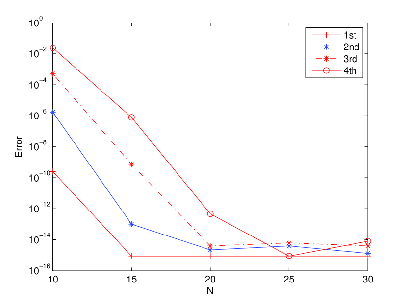
Refer to caption
Figure 1: Errors between numerical and reference solution of the TE mode for l=1𝑙1l=1.
Refer to caption
Figure 2: Errors between numerical and reference solutions of the TM mode for l=1𝑙1l=1.
Refer to caption
Figure 3: Errors between numerical and reference solutions of the TE mode for l=2𝑙2l=2.
Refer to caption
Figure 4: Errors between numerical and reference solutions of the TM mode for l=2𝑙2l=2.
Refer to caption
Figure 5: Errors between numerical and reference solutions of the TE mode for l=3𝑙3l=3.
Refer to caption
Figure 6: Errors between numerical and reference solutions of the TM mode for l=3𝑙3l=3.

6.2 Inhomogeneous medium n𝑛n

We take R=1𝑅1R=1, n=8+4r2𝑛84superscript𝑟2n=8+4r^{2}, and l=1𝑙1l=1 in our examples. Numerical results of the first four eigenvalues with different N𝑁N are listed in Table 6.8 for the TE mode and in Table 6.9 for the TM mode, respectively.

Table 6.8 The first four eigenvalues of the TE mode for l=1𝑙1l=1 and different N𝑁N in unit ball N 1st1𝑠𝑡1st 2nd2𝑛𝑑2nd 3rd3𝑟𝑑3rd 4th4𝑡4th 10 1.924760241224309 3.066320509754762 4.953581565194202 6.219217568046522 15 1.924760240239596 3.066318451356159 4.944962746965171 6.162042706007884 20 1.924760240239595 3.066318451356097 4.944962719618220 6.162013704025296 25 1.924760240239596 3.066318451356097 4.944962719618172 6.162013703949516 30 1.924760240239597 3.066318451356096 4.944962719618174 6.162013703949522

Table 6.9 The first four eigenvalues of the TM mode for l=1𝑙1l=1 and different N𝑁N in unit ball N 1st1𝑠𝑡1st 2nd2𝑛𝑑2nd 3rd3𝑟𝑑3rd 4th4𝑡4th 10 1.546722576754737 3.418052693123285 4.366864963075772 4.640915773722154 15 1.546722576768443 3.418109299464758 4.616102608978945 6.423176009030875 20 1.546722576768448 3.418109299467635 4.616102624493460 6.425723290604534 25 1.546722576768440 3.418109299467642 4.616102624493454 6.425723292013815 30 1.546722576768443 3.418109299467622 4.616102624493481 6.425723292013920

We see from Tables 6.8-6.9 that numerical eigenvalues achieve at least thirteen-digit accuracy with N25𝑁25N\geq 25. Here again, we use numerical solutions with N=60𝑁60N=60 as reference solutions and plot the errors in Figure 7-8.
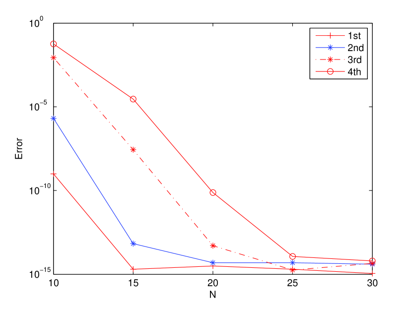
Refer to caption
Figure 7: Errors between numerical and reference solutions of the TE mode for l=1𝑙1l=1.
Refer to caption
Figure 8: Errors between numerical and reference solutions of the TM mode for l=1𝑙1l=1.

7 Conclusions

In summary, the method developed in this paper is a first but important step towards a robust and accurate algorithm for more general transmission eigenvalue problems which will be the subject of our future work.

References

  • [1] F. CAKONI AND D. COLTON, Qualitative methods in inverse scattering theory, Springer Berlin Heidelberg, 2006.
  • [2] F. CAKONI, D. COLTON, AND P. MONK, The Linear Sampling Method in Inverse Electromagnetic Scattering, SIAM, 2011.
  • [3] J. SUN AND L. XU, Computation of Maxwell s transmission eigenvalues and its applications in inverse medium problems, Inverse Problems, 29(10)(2013), pp. 104013.
  • [4] F. CAKONI, D. COLTON, AND P. MONK, On the use of transmission eigenvalues to estimate the index of refraction from far field data, Inverse Problems, 23(2)(2017), pp. 507–522.
  • [5] F. CAKONI, D. COLTON, P. MONK, AND J. SUN, The inverse electromagnetic scattering problem for anisotropic media, Inverse Problems, 26(2010), pp. 074004.
  • [6] J. AN AND J. SHEN, Efficient spectral methods for transmission eigenvalues and estimation of the index of refraction, J. Math. Study, 1(1)(2014), pp. 1–20.
  • [7] H. HADDAR, The interior transmission problem for anisotropic maxwell s equations and its applications to the inverse problem, Math. Methods in Appl. Sci., 27(18)(2004), pp. 2111–2129.
  • [8] J. SUN, Estimation of transmission eigenvalues and the index of refraction from Cauchy data , Inverse Problems, 27(1998), pp. 015009.
  • [9] F. CAKONI, D. COLTON, AND H. HADDAR, On the determination of dirichlet or transmission eigenvalues from far field data, Comptes Rendus Mathematique, 348(7-8)(2010), pp. 379 C383.
  • [10] P. MONK AND J. SUN, Finite element methods for Maxwell’s transmission eigenvalues, SIAM J. Sci. Comput., 34(3)(2012), pp. B247-B264.
  • [11] T. M. HUANG, W. Q. HUANG AND W. W. LIN, A robust numerical algorithm for computing Maxwell’s transmission eigenvalue problems, SIAM J. Sci. Comput., 37(5)(2015), pp. A2403-A2423.
  • [12] F. CAKONI AND H. HADDAR, On the existence of transmission eigenvalues in an inhomogeneous medium, Applicable Analysis, 88(4)(2009), pp. 475-493.
  • [13] L. MA, J. SHEN AND L. L. WANG, Spectral approximation of time-harmonic Maxwell equations in three-dimensional exterior domains, Int. J. Numer. Anal. Mod., 12(2)(2015), pp. 1-18.
  • [14] E. L. HILL, The theory of vector spherical harmonics, Amer. J. Phys., 22(1954), pp. 211-214.
  • [15] T. HAGSTROM AND S. LAU, Radiation boundary conditions for Maxwell s equations: a review of accurate time-domain formulations, J. Comput. Math., 25(3)(2007), pp. 305-336.
  • [16] R. G. BARRERA, G. A. ESTEVEZ, AND J. GIRALDO, Vector spherical harmonics and their application to magnetostatics, European Journal of Physics , 6(1985), pp. 287.
  • [17] J. SHEN , T. TANG, AND L. L. WANG, Spectral methods: algorithms, analysis and applications, Springer Science and Business Media, 2011.
  • [18] M. S. MIN AND D. GOTTLIEB, On the convergence of the Fourier approximation for eigenvalues and eigenfunctions of discontinuous problems, SIAM J. Numer. Anal., 40(6)(2003), pp. 2254-2269.
  • [19] J. SHEN AND T. TANG, Spectral and high-order methods with applications, Science Press, 2006.
  • [20] G. H. GOLUB AND C. F. VAN LOAN, Matrix Computations, The John Hopkins University Press, Baltimore, 1989.
  • [21] Y. KWAN AND J. SHEN, An efficient direct parallel elliptic solver by the spectral element metho, J. Comput. Phys., 225(2007),pp:1721-1735.