Functional Regression on Manifold with Contamination

Abstract

We propose a new method for functional nonparametric regression with a predictor that resides on a finite-dimensional manifold but is only observable in an infinite-dimensional space. Contamination of the predictor due to discrete/noisy measurements is also accounted for. By using functional local linear manifold smoothing, the proposed estimator enjoys a polynomial rate of convergence that adapts to the intrinsic manifold dimension and the contamination level. This is in contrast to the logarithmic convergence rate in the literature of functional nonparametric regression. We also observe a phase transition phenomenon regarding the interplay of the manifold dimension and the contamination level. We demonstrate that the proposed method has favorable numerical performance relative to commonly used methods via simulated and real data examples.

1 Introduction

Regression with a functional predictor is of central importance in the field of functional data analysis, the field that has been advanced by Ramsay & Silverman (1997, 2002) and many others. Early development of functional regression focuses on functional linear models (Cardot et al., 1999; Yao et al., 2005b; Yuan & Cai, 2010). Extensions of linear models include generalized linear regression (Cardot & Sarda, 2005; Müller & Stadtmüller, 2005), additive models (Müller & Yao, 2008), quadratic models (Yao & Müller, 2010), among others. These works prescribe specific forms of the regression model, and are regarded as functional parametric regression models (Ferraty & Vieu, 2006) that entail efficient estimation procedures and hence are well studied in the literature.

In contrast, functional nonparametric regression that does not impose structural constraints on the regression function has received less attention. The first landmark development of nonparametric functional data analysis is the monograph of Ferraty & Vieu (2006). Recent advances in this direction include the Nadaraya–Watson estimator (Ferraty et al., 2012) and the $k$-nearest-neighbor estimator (Kudraszow & Vieu, 2013). The development of functional nonparametric regression is hindered by a theoretical barrier that is formulated in Mas (2012) and is linked to the small ball probability problem (Delaigle & Hall, 2010). Essentially, in a rather general setting, the minimax rate of nonparametric regression on a generic functional space is slower than any polynomial of the sample size, which differs markedly from the polynomial minimax rates for many functional parametric regression procedures (e.g. Hall & Keilegom, 2007; Yuan & Cai, 2010, for functional linear regression). These endeavors on functional nonparametric regression do not exploit the intrinsic structure that is common in practice. For instance, Chen & Müller (2012) suggested that functional data often possess a low-dimensional manifold structure which can be utilized for more efficient representation. By contrast, we exploit the nonlinear low-dimensional structure for functional nonparametric regression.

Our method, which we call functional regression on manifold, assumes the model

$$Y=g(X)+\varepsilon,$$ (1)

where $Y$ is a scalar response, $X$ is a functional predictor sampled from an unknown manifold $\mathcal{M}$, $\varepsilon$ is the error term independent of $X$, and $g$ is some unknown functional to be estimated. In reality, the functional predictor $X$ is rarely fully observed. To accommodate this common practice, we assume that $X$ is recorded at a grid of points with noise. The model (1) features a manifold structure $\mathcal{M}$ that underlies the functional predictor $X$ and is assumed to be a finite-dimensional but potentially nonlinear submanifold of the function space $\mathcal{L}^{2}(D)$, the space of square integrable functions defined on a compact domain $D\subset\real$. For a background on both finite-dimensional and infinite-dimensional manifolds, we refer readers to Lang (1995) and Lang (1999).

Data analysis with a manifold structure has been extensively studied in the statistical literature. For example, techniques have been invented to learn an unknown manifold based on a point cloud, such as locally linear embedding (Roweis & Saul, 2000; Wu & Wu, 2018), isomap (Tenenbaum et al., 2000), t-SNE (van der Maaten & Hinton, 2008), among many others. Supervised learning on an unknown manifold has also been investigated, such as estimation of functions defined on a manifold (Aswani et al., 2011; Cheng & Wu, 2013; Sober et al., 2019) and estimation of the gradient of such functions (Mukherjee et al., 2010). In addition, data analysis on a known manifold has been studied, such as fundamentals related to the Fréchet mean (Bhattacharya & Patrangenaru, 2003, 2005; Bhattacharya & Lin, 2017), manifold-valued function estimation (Yuan et al., 2012; Lin et al., 2016; Cornea et al., 2017; Lin et al., 2019), manifold-valued principal component analysis (Huckemann et al., 2010; Panaretos et al., 2014), classification on manifolds (Yao & Zhang, 2019+), and nonparametric manifold-valued inference (Patrangenaru & Ellingson, 2015).

However, the literature specifically relating functional data to manifolds is scarce. Zhou & Pan (2014) investigated functional principal component analysis on an irregular domain. Chen & Müller (2012) and Lila & Aston (2016) considered the representation and principal component analysis of functional data sampled from a manifold. Manifold-valued random functions were studied by Su et al. (2014), Dai & Müller (2018) and Lin & Yao (2019). To the best of our knowledge, we are the first to consider a manifold structure in functional regression where a global representation of the low-dimensional functional predictor $X$ can be inefficient. For illustration, Example 1 in Supplementary Material exhibits a random process taking values in a one-dimensional submanifold of $\mathcal{L}^{2}([0,1])$ while having an infinite number of components in its Karhunen–Loève expansion.

When estimating the regression functional $g$ in (1), we explicitly account for the hidden manifold structure by estimating the tangent spaces of the manifold. Specifically, we first recover the observed functional predictors from their discrete/noisy measurements, and then adopt the local linear manifold smoothing (Cheng & Wu, 2013). While our approach and the one of Cheng & Wu (2013) share the same intrinsic manifold setup, they fundamentally differ in the ambient aspect, which raises challenging issues unique to functional data. First, functional data naturally live in an infinite-dimensional ambient space, while the Euclidean data considered by Cheng & Wu (2013) have a finite ambient dimension. Second, the effect of noise/sampling in the observed functional data needs to be explicitly treated, since functional data are discretely and noisily recorded in practice, which then introduces contamination of the functional predictor. This contamination issue is not encountered in Cheng & Wu (2013), or is only considered for linear regression of multivariate data (Aswani et al., 2011; Loh & Wainwright, 2012). Moreover, the contamination has an intrinsic dimension that grows with the sample size and thus is coupled with the ambiently infinite dimensionality.

The main contributions of this article are as follows. First, by exploiting structural information of the predictor, our proposal entails an effective estimation procedure that adapts to the unknown manifold structure and the contamination level while maintains the flexibility of functional nonparametric regression. Second, by careful theoretical analysis, we confirm that the regression functional $g$ can be estimated at a polynomial convergence rate of the sample size, especially when only the contaminated functional predictors are available. This provides a new angle to functional nonparametric regression that is subject to a logarithmic rate (Mas, 2012). Third, the contamination on predictors is explicitly treated and is shown to be an integrated part of the convergence rate, which has not been well studied even in classical functional linear regression (Hall & Keilegom, 2007). Finally, we discover that, the polynomial convergence rate exhibits a phase transition phenomenon, depending on the interplay between the manifold dimension and the contamination level. This type of phase transition has not yet been discovered in functional regression, and shares at least the same importance of those concerning estimation of mean/covariance functions (e.g. Cai & Yuan, 2011; Zhang & Wang, 2016). In addition, during our theoretical development, we obtain some results that are generally useful with their own merit, such as the consistency of the estimated intrinsic dimension and tangent spaces of the manifold in the presence of contamination.

2 Estimation of Functional Regression on Manifold

2.1 Step I: Recovery of Functional Data

We assume that each predictor $X_{i}$ is observed at $m_{i}$ design points $T_{i1},\ldots,T_{im_{i}}\in D$. Denote the observed value at $T_{ij}$ by $X_{ij}^{\ast}=X_{i}(T_{ij})+\zeta_{ij}$, where $\zeta_{ij}$ is random noise with mean zero and is independent of all $X_{i}$ and $T_{ij}$. The collection ${\mathbb{X}}_{i}=\{(T_{i1},X_{i1}^{\ast}),\ldots,(T_{im_{i}},X_{im_{i}}^{\ast})\}$ represents all measurements for the realization $X_{i}$, and $\{\mathbb{X}_{1},\ldots,\mathbb{X}_{n}\}$ constitutes the observed data for the predictor. We shall clarify that, although each trajectory $X_{i}$ as a whole function resides on the manifold $\mathcal{M}$, the $m_{i}$-dimensional vector $\mathbb{V}_{i}=(X_{i}(T_{i1}),\ldots,X_{i}(T_{im_{i}}))$ does not. Consequently, the manifold assumption in Cheng & Wu (2013) is violated for $\mathbb{V}_{i}$.

When $\inf_{i}m_{i}$ is sufficiently large or grows with the sample size, a scenario commonly referred to as the dense design, we may recover each function $X_{i}$ based on the observed data $\mathbb{X}_{i}$ by individual smoothing estimation. Popular smoothing techniques include the local linear smoother (Fan, 1993) and spline smoothing (Ramsay & Silverman, 2005), among others. By applying one of these methods, we obtain an estimate $\hat{X}_{i}$ of $X_{i}$, referred to as the contaminated version of $X_{i}$ that is used in the subsequent steps to estimate $g$. To be specific, we consider the local linear estimate of $X_{i}(t)$ given by $\hat{b}_{1}$ with

$$(\hat{b}_{1},\hat{b}_{2})=\underset{(b_{1},b_{2})\in{}^{2}}{\arg\min}\frac{1}{m_{i}}\sum_{j=1}^{m_{i}}\left\{X_{ij}^{\ast}-b_{1}-b_{2}(T_{ij}-t)\right\}^{2}K\left(\frac{T_{ij}-t}{h_{i}}\right),$$ (2)

where $K$ is a compactly supported symmetric density function and $h_{i}$ is the bandwidth. Calculation shows that $\hat{b}_{1}=(R_{0}S_{2}-R_{1}S_{1})/(S_{0}S_{2}-S_{1}^{2})$, where for $r=0,1$ and $2$,

$$S_{r}(t)=\frac{1}{m_{i}h_{i}}\sum_{j=1}^{m_{i}}K\left(\frac{T_{ij}-t}{h_{i}}\right)\left(\frac{T_{ij}-t}{h_{i}}\right)^{r},R_{r}(t)=\frac{1}{m_{i}h_{i}}\sum_{j=1}^{m_{i}}K\left(\frac{T_{ij}-t}{h_{i}}\right)\left(\frac{T_{ij}-t}{h_{i}}\right)^{r}X_{ij}^{\ast}.$$

The estimate $\hat{b}_{1}$ does not have a finite mean squared error, as its denominator is zero with a positive probability for a finite sample. To overcome this issue, we adopt the technique of ridging (Fan, 1993; Seifert & Gasser, 1996; Hall & Marron, 1997) to estimate $X_{i}(t)$ by the following ridged local linear estimate

$$\hat{X}_{i}(t)=\frac{R_{0}S_{2}-R_{1}S_{1}}{S_{0}S_{2}-S_{1}^{2}+\delta 1_{\{|S_{0}S_{2}-S_{1}^{2}|<\delta\}}},$$ (3)

where $\delta>0$ is a sufficiently small constant that depends on $m_{i}$, e.g., $\delta={m}_{i}^{-2}$.

When $\sup_{i}m_{i}$ is relatively small or bounded by a constant, a scenario commonly referred to as the sparse design, to recover $X_{i}$, the procedure proposed by Yao et al. (2005a) can be adopted to recover individual functions. We refer readers to Supplementary Material for the details of such procedure.

2.2 Step II: Estimation of the Manifold Dimension and Tangent Space

To characterize the manifold structure, we shall first estimate the intrinsic dimension $d$ of the manifold $\mathcal{M}$. We adopt the maximum likelihood estimator proposed by Levina & Bickel (2004), substituting the unobservable $X_{i}$ with the contaminated version $\hat{X}_{i}$. For a given $x\in\mathcal{M}$, define $\hat{G}_{i}(x)=\|x-\hat{X}_{i}\|_{\mathcal{L}^{2}}$ and let $\hat{G}_{(k)}(x)$ be the $k$th order statistic of $\hat{G}_{1}(x),\ldots,\hat{G}_{n}(x)$. Then the intrinsic dimension $d$ is estimated by

$$\hat{d}=\frac{1}{k_{2}-k_{1}+1}\sum_{k=k_{1}}^{k_{2}}\hat{d}_{k},$$ (4)

with

$$\hat{d}_{k}=\frac{1}{n}\sum_{i=1}^{n}\hat{d}_{k}(\hat{X}_{i}),\qquad\hat{d}_{k}(x)=\left\{\frac{1}{k-1}\sum_{j=1}^{k-1}\log\frac{\hat{G}_{(k)}(x)+\Delta}{\hat{G}_{(j)}(x)+\Delta}\right\}^{-1},$$ (5)

where $\Delta$ is a positive constant depending on $n$, and $k_{1},k_{2}$ are tuning parameters. This $\Delta$ regularizes $\hat{d}_{k}(x)$ in order to overcome the additional variability introduced by the contamination on the predictor. We conveniently set $\Delta=1/\log\bar{m}$ with $\bar{m}=n^{-1}\sum_{i=1}^{n}m_{i}$, while refer readers to Levina & Bickel (2004) for the choice of $k_{1}$ and $k_{2}$. When the observed data are sparsely sampled, the distance $\hat{G}_{i}(x)$ can be better estimated by the procedure of Peng & Müller (2008).

Now we proceed to estimate the tangent space at the given point $x$ as follows.

• A neighborhood of $x$ is determined by a tuning parameter $h_{pca}>0$, denoted by $\hat{\mathcal{N}}_{\mathcal{L}^{2}}(h_{pca},x)=\{\hat{X}_{i}:\|x-\hat{X}_{i}\|_{\mathcal{L}^{2}}<h_{pca},\;i=1,\ldots,n\}$.

• Compute the local empirical covariance function

  $$\hat{\mathcal{C}}_{x}(s,t)=\frac{1}{|\hat{\mathcal{N}}_{\mathcal{L}^{2}}(h_{pca},x)|}\sum_{\hat{X}\in\hat{\mathcal{N}}_{\mathcal{L}^{2}}(h_{pca},x)}\{\hat{X}(s)-\hat{\mu}_{x}(s)\}\{\hat{X}(t)-\hat{\mu}_{x}(t)\}$$ (6)

  and obtain the eigenfunctions $\hat{\varphi}_{1},\hat{\varphi}_{2},\ldots,\hat{\varphi}_{\hat{d}}$ corresponding to the first $\hat{d}$ leading eigenvalues, where $\hat{\mu}_{x}=|\hat{\mathcal{N}}_{\mathcal{L}^{2}}(h_{pca},x)|^{-1}\sum_{\hat{X}\in\hat{\mathcal{N}}_{\mathcal{L}^{2}}(h_{pca},x)}\hat{X}$ is the local mean function and $|\hat{\mathcal{N}}_{\mathcal{L}^{2}}(h_{pca},x)|$ denotes the number of observations in $\hat{\mathcal{N}}_{\mathcal{L}^{2}}(h_{pca},x)$.

• Estimate the tangent space at $x$ by $\widehat{T_{x}\mathcal{M}}=\mathrm{span}\{\hat{\varphi}_{1},\hat{\varphi}_{2},\ldots,\hat{\varphi}_{\hat{d}}\}$, the linear space spanned by the first $\hat{d}$ estimated eigenfunctions.

2.3 Step III: Local Linear Regression on the Tangent Space

Finally, we utilize the local manifold structure by projecting all $\hat{X}_{i}$ onto the estimated tangent space $\widehat{T_{x}\mathcal{M}}$ and obtain the local coordinate $\hat{\xi}_{i}=(\langle\hat{X}_{i},\hat{\varphi}_{1}\rangle,\ldots,\langle\hat{X}_{i},\hat{\varphi}_{\hat{d}}\rangle)^{T}$ for $\hat{X}_{i}$. Then, the estimate of $g(x)$ is given by

$$\hat{g}(x)={e}_{1}^{T}(\hat{Q}^{T}\hat{{W}}\hat{Q})^{-1}\hat{Q}^{T}\hat{{W}}\mathcal{Y},\quad\quad\hat{Q}=\begin{pmatrix}1&1&\cdots&1\\ \hat{\xi}_{1}&\hat{\xi}_{2}&\cdots&\hat{\xi}_{n}\end{pmatrix}^{T},$$ (7)

$\hat{{W}}=\mathrm{diag}(K_{h_{reg}}(\|x-\hat{X}_{1}\|_{\mathcal{\mathcal{L}}^{2}}),K_{h_{reg}}(\|x-\hat{X}_{2}\|_{\mathcal{\mathcal{L}}^{2}}),\ldots,K_{h_{reg}}(\|x-\hat{X}_{n}\|_{\mathcal{\mathcal{L}}^{2}}))$ with $K_{h}(t)=K(t/h)/h^{\hat{d}}$ and the bandwidth $h_{reg}$, $\mathcal{Y}=(Y_{1},\ldots,Y_{n})^{T}$, and ${e}_{1}^{T}=(1,0,\ldots,0)$ is an $n\times 1$ vector. Here, the matrix $\hat{Q}$ incorporates the estimated geometric structure that is encoded by the local eigenbasis $\hat{\varphi}_{1},\ldots,\hat{\varphi}_{\hat{d}}$. We emphasize that, in the above estimation procedure which is illustrated by the diagram in the left panel of Figure 1, all steps are based on the contaminated sample $\{\hat{X}_{1},\ldots,\hat{X}_{n}\}$, rather than the unavailable functions $X_{1},\ldots,X_{n}$. When the predictor $x$ is also only measured at $m_{x}$ discrete points $t_{1},\ldots,t_{m_{x}}$, we impute it by the procedures in Section 2.1, and replace $x$ in (5)–(7) with the imputed curve $\tilde{x}$ to obtain an estimate of $g(\tilde{x})$.

2.4 Tuning Parameter Selection

There are several tuning parameters to be determined in our estimation procedure. For the parameters $k_{1}$ and $k_{2}$ in (4) to estimate the intrinsic dimension, $k_{1}=10$ and $k_{2}=20$ are suggested by Levina & Bickel (2004). However, we found that $k_{1}=20$ and $k_{2}=30$ work better generally in our setting, perhaps partially due to the contamination that requires a relatively larger local neighborhood to offset.

For the individual smoothing presented in Section 2.1, we adopt the following leave-one-out cross-validation to select the bandwidth $h_{i}$ (Fan & Gijbels, 1996; Lee & Solo, 1999). Let $\hat{X}_{i,h,-j}(x)$ be the leave-one-out estimate of $X_{i}(t)$, i.e., the estimate computed according to (3) using all of $(T_{i1},X_{i1}^{\ast}),\ldots,(T_{im_{i}},X_{im_{i}}^{\ast})$ but $(T_{ij},X_{ij}^{\ast})$. We then select $h_{i}$ from a pool of candidates to minimize the cross-validation error $\textsc{cv}(h)=\sum_{j=1}^{m_{i}}\{X_{ij}^{\ast}-\hat{X}_{i,h,-j}(T_{ij})\}^{2}.$

For the bandwidths $h_{pca}$ in (6) and $h_{reg}$ in (7), we choose the pair $(h_{pca},h_{reg})$ from a pool $\mathbb{H}$ of candidate pairs to minimize the following leave-one-out cross-validation error $\textsc{cv}(h_{pca},h_{reg})=\sum_{i=1}^{n}\{Y_{i}-\hat{g}_{h_{pca},h_{reg},-i}(\hat{X}_{i})\}^{2},$ where $\hat{g}_{h_{pca},h_{reg},-i}$ denotes the leave-one-out estimate of $g$ with parameters $h_{pca},h_{reg}$ without using the pair $(\hat{X}_{i},Y_{i})$. The pool $\mathbb{H}$ shall be constructed in the way that every $\hat{\mathcal{N}}_{\mathcal{L}^{2}}(h_{pca},\hat{X}_{i})$ contains at least $\hat{d}+1$ samples for every pair $(h_{pca},h_{reg})$ in $\mathbb{H}$ to ensure sufficient data for local estimation.

Figure 1: Illustration of functional regression on a manifold (left panel) and illustration of the asymptotic result of (9) for $d=2$ (right panel).

3 Theoretical Properties

We focus on the scenario that $\inf_{i}m_{i}$ increases with the sample size $n$, while leave the one that $\sup_{i}m_{i}\leq m_{0}<\infty$ for future research due to elevated challenges. Without loss of generality, assume $m_{i}\asymp m$ where $a_{n}\asymp b_{n}$ denotes $0<\lim\inf a_{n}/b_{n}<\lim\sup a_{n}/b_{n}<\infty$. We further assume that $\zeta_{ij}$, and similarly, $T_{ij}$ and $X_{i}$, are independently and identically distributed, while emphasize that the development below can be modified to accommodate fixed designs, weak dependence and/or heterogeneous distributions. This generality will require considerably heavier technicalities without adding further insight, and is not pursued here.

The discrepancy between $\hat{X}_{i}$ and $X_{i}$, quantified by $\|\hat{X}_{i}-X_{i}\|_{\mathcal{L}^{2}}$, is termed the contamination of $X_{i}$. The decay of this contamination is intimately linked to the consistency of our estimates of the intrinsic dimension, the tangent space, and eventually the regression functional $g(x)$. Moreover, the convergence rate of $\hat{g}(x)$ is found to exhibit a phase transition phenomenon depending on the interplay between the intrinsic dimension and the decay of contamination. To set the stage, we start with a property of contamination in recovery of functional data by the individual smoothing approach in Section 2.1. Specifically, we study the $p$th moment of contamination when $\hat{X}_{i}$ is the ridged local linear estimate in (3). Our result below for an arbitrary $p$th moment is not present in the literature (e.g., Fan, 1993, for $p=2$ only).

Let $\Sigma(\nu,L)$ denote the Hölder class with an exponent $\nu$ and an Hölder constant $L$, which represents the set of $\ell=\lfloor\nu\rfloor$ times differentiable functions $F$ whose derivative $F^{(\ell)}$ satisfies $|F^{(\ell)}(t)-F^{(\ell)}(s)|\leq L|t-s|^{\nu-\ell}$ for $s,t\in D,$ where $\lfloor\nu\rfloor$ denotes the largest integer strictly smaller than $\nu$. We require the following mild assumptions, and assume $h_{i}\asymp h_{0}$ without loss of generality.

• $K$ is a differentiable kernel with a bounded derivative, $\int_{-1}^{1}K(u)du=1$, $\int_{-1}^{1}uK(u)du=0$, and $\int_{-1}^{1}|u|^{p}K(u)du<\infty$ for all $p>0$.

• The sampling density $f_{T}$ is bounded away from zero and infinity, i.e., for some constants $C_{T,1},C_{T,2}\in(0,\infty)$, $C_{T,1}=\inf_{t\in D}f_{T}(t)\leq\sup_{t\in D}f_{T}(t)=C_{T,2}$.

• $X\in\Sigma(\nu,L_{X})$, where $L_{X}>0$ is a random quantity and the constant $\nu\in(0,2]$ quantifies the smoothness of the process.

• For all $r\geq 1$, ${E}\sup_{t}|X(t)|^{r}<\infty$, ${E}(L_{X})^{r}<\infty$ and ${E}|\zeta|^{r}<\infty$.

The condition ${E}\sup_{t}|X(t)|^{r}<\infty$ holds rather generally (Li & Hsing, 2010; Zhang & Wang, 2016), compared to a stronger assumption on $X$ given in (A.1) of Hall et al. (2006). The following proposition is an immediate consequence of Lemma S.1 in the Supplementary Material, and hence its proof is omitted.

Proposition 3.1.

For any $p\geq 1$, assume ${E}|\zeta|^{p}<\infty$. Under the assumptions (A1)–(A3), for the estimate $\hat{X}$ in (3) with $h_{0}\asymp m^{-\frac{1}{2\nu+1}}$ and $\delta=m^{-2}$, we have

$$\{{E}(\|\hat{X}-X\|_{\mathcal{L}^{2}}^{p}\mid X)\}^{1/p}=O(m^{-\frac{\nu}{2\nu+1}})\left\{\sup_{t}|X(t)|+L_{X}\right\}.$$ (8)

Furthermore, if the assumption (A4) also holds, then $\left({E}\|\hat{X}-X\|_{\mathcal{L}^{2}}^{p}\right)^{1/p}=O(m^{-\frac{\nu}{2\nu+1}}).$

When $X$ is deterministic as in nonparametric regression, the rate in (8) for $p=2$ coincides with that in Tsybakov (2008). In addition, the $p$th order of the contamination $\|\hat{X}_{i}-X_{i}\|_{\mathcal{L}^{2}}$ decays at a polynomial rate that depends on $\nu$, but not the order $p$.

To analyze the asymptotic property of $\hat{g}(x)$, we make the following assumptions.

• The probability density $f$ of $X$ on $\mathcal{M}$ satisfies $C_{f,1}=\inf_{x\in\mathcal{M}}f(x)\leq\sup_{x\in\mathcal{M}}f(x)=C_{f,2}$ for some constants $0<C_{f,1}\leq C_{f,2}<\infty$.

• The regression functional $g$ has a bounded second derivative.

For (B1), since the functional predictor resides on a low-dimensional manifold, the existence of a density can be safely assumed. We also make the following assumption on the imputed trajectories in Section 2.1.

• $\hat{X}_{1},\ldots,\hat{X}_{n}$ are independently and identically distributed. For some $\beta\in(0,\infty)$ and all $p\geq 1$, $\{{E}(\|\hat{X}-X\|_{\mathcal{L}^{2}}^{p}\mid X)\}^{1/p}\leq C_{p}m^{-\beta}\eta(X)$ for some constant $C_{p}$ depending only on $p$ and some nonnegative function $\eta(X)$ depending only on $X$ such that ${E}\{\eta(X)\}^{p}<\infty$.

Under the assumptions (A1)–(A4), by Proposition 3.1, the imputed functions $\hat{X}_{1},\ldots,\hat{X}_{n}$ by individual smoothing via local linear estimation (3) satisfies (B3) with $\beta=\nu/(2\nu+1)$. Therefore, (B3) could be replaced with the more concrete assumptions (A1)–(A4). It can be relaxed to accommodate heterogeneous data distributions and weakly dependent functional data by modifying our proofs. Also, it is possible to accommodate imputed functions that are attained by borrowing information across individuals (e.g., Yao et al., 2005a), which is beyond our scope here and can be a topic of future research.

The contamination of the predictor $X$ renders the true neighborhood $\mathcal{N}_{\mathcal{L}^{2}}(h_{pca},x)=\{X_{i}:\|X_{i}-x\|_{\mathcal{L}^{2}}<h_{pca}\}$ inaccessible. However, we can show that the contaminated one $\hat{\mathcal{N}}_{\mathcal{L}^{2}}(h_{pca},x)$ is a good estimate; see Section S.2 and Lemma 8 in Supplementary Material for details. Consequently, the local manifold structure can be consistently estimated in the sense of the following theorem.

Theorem 3.2.

Suppose that the assumptions (B1) and (B3) hold.

1. $\hat{d}$ is a consistent estimator of $d$ when $\min\{k_{1},k_{2}\}\rightarrow\infty$ and $\max\{k_{1},k_{2}\}/m\rightarrow 0$.

2. If $h_{pca}\rightarrow 0$ and $h_{pca}\gtrsim\max\{m^{-\beta+\epsilon},n^{-1/(d+2)}\}$ for an arbitrarily small but fixed constant $\epsilon>0$, then the eigenbasis $\{\hat{\varphi}_{k}\}_{k=1}^{d}$ derived from $\hat{\mathcal{C}}_{x}$ in (6) is close to an orthonormal basis $\{\phi_{k}\}_{k=1}^{d}$ of $T_{x}\mathcal{M}$, in the sense that, for each $x\in\mathcal{M}$,

   $$\hat{\varphi}_{k}=\phi_{k}+O_{P}(h_{pca}^{3/2}){u}_{k}+O_{P}(h_{pca}){u}_{k}^{\perp}\quad(k=1,\ldots,d),$$ (9)

   where ${u}_{k}\in T_{x}\mathcal{M}$, ${u}_{k}^{\perp}\perp T_{x}\mathcal{M}$, and $\|{u}_{k}\|_{\mathcal{L}^{2}}=\|{u}_{k}^{\perp}\|_{\mathcal{L}^{2}}=1$.

In light of Theorem 3.2(a), we shall from now on present the subsequent results by conditioning on the event $\hat{d}=d$. For part (b) that is illustrated in the right panel of Figure 1, the condition $h_{pca}\gtrsim m^{-\beta+\epsilon}$ suggests that $h_{pca}$ shall be larger than the contamination by an arbitrarily small polynomial order of $m$. This is required to ensure that the discrepancy between the estimated local neighborhood $\hat{N}_{\mathcal{L}^{2}}(h_{pca},x)$ and the uncontaminated neighborhood $\mathcal{N}_{\mathcal{L}^{2}}(h_{pca},x)=\{X_{i}:\|x-X_{i}\|_{\mathcal{L}^{2}}<h_{pca},i=1,\ldots,n\}$ is asymptotically negligible, suggested by Lemma 8 in Supplementary Material. The curvature at $x$ is a constant that is absorbed into the $O_{P}$ terms, and thus does not influence the asymptotic rate. However, practically it is often more difficult to estimate the tangent structure at a point with larger curvature.

We are ready to state the results on the estimated regression functional. Recall that $\hat{g}(x)$ in (7) is obtained by applying the local linear smoother to the coordinates of contaminated predictors within the estimated tangent space at $x$. It is well known that the local linear estimator does not suffer from boundary effects, i.e., the first order behavior of the estimator on the boundary is the same as in the interior (Fan, 1992). However, the contamination of the predictor has different impact, and we shall address the interior and boundary cases separately. Denote $\mathscr{X}=\{(X_{1},\hat{X}_{1}),\ldots,(X_{n},\hat{X}_{n})\}$ and $\mathcal{M}_{h}=\{x\in\mathcal{M}:\inf_{y\in\partial\mathcal{M}}\mathfrak{d}(x,y)\leq h\}$, where $\partial\mathcal{M}$ denotes the boundary of $\mathcal{M}$ and $\mathfrak{d}(\cdot,\cdot)$ denotes the distance function on $\mathcal{M}$. For points sufficiently far away from the boundary of $\mathcal{M}$, we have the following result about the convergence rate of the estimator $\hat{g}(x)$.

Theorem 3.3.

Assume that (A1) and (B1)–(B3) hold. Let $x\in\mathcal{M}\backslash\mathcal{M}_{h_{reg}}$ and $h_{pca}$ satisfies the conditions of Theorem 3.2(b). For an arbitrarily small but fixed constant $\epsilon>0$, suppose that $h_{reg}\rightarrow 0$, $h_{reg}>h_{pca}$, and $\min\{nh_{reg},m^{\beta}h^{5/3+\epsilon}_{reg}\}\rightarrow\infty$. Then

$${E}\left[\left\{\hat{g}(x)-g(x)\right\}^{2}\mid\mathscr{X}\right]=O_{P}\left(h^{4}+\frac{1}{m^{2\beta}h_{reg}^{2+2\epsilon}}+\frac{1}{nh^{d}}\right).$$ (10)

In addition, if $h_{pca}\asymp\max\{m^{-\beta},n^{-1/(d+2)}\}$, and $h_{reg}\asymp n^{-1/(d+4)}$ when $m\gtrsim n^{(3+\epsilon)/\{\beta(d+4)\}}$ and $h_{reg}\asymp m^{-\beta/(3+\epsilon)}$ otherwise, then

$${E}\left[\left\{\hat{g}(x)-g(x)\right\}^{2}\mid\mathscr{X}\right]=O_{P}\left(n^{-\frac{4}{d+4}}+m^{-\frac{4\beta}{3+\epsilon}}\right).$$ (11)

We emphasize the following observations from this theorem. First, according to our analysis in Supplementary Material, the first two terms on the right hand side of (10) correspond to the bias while the last term stems from the variability of the estimator. This suggests that, under the conditions of the theorem, the contamination has impact on the asymptotic bias but not the variance. Second, the convergence rate of $\hat{g}(x)$ is a polynomial of the sample size $n$ and the sampling rate $m$. This is in contrast with traditional functional nonparametric regression methods that do not exploit the intrinsic structure and thus cannot reach a polynomial rate of convergence.

Third, the rate in (11) consists of two terms, one related to the intrinsic dimension $d$ and the sample size $n$, and the other related to $m$ and $\beta$ that together characterize the contamination of the predictor. As $\epsilon>0$ is arbitrary, the transition of these two terms occurs at the rate $\mathfrak{m}_{0}\asymp n^{3/\{\beta(d+4)\}}$. When the sampling rate falls below $\mathfrak{m}_{0}$, the contamination term dominates the convergence rate in (11). Otherwise, the intrinsic dimension and sample size determine the rate. This phase transition, although sharing the similar spirit of Cai & Yuan (2011) and Zhang & Wang (2016), has a different interpretation, as follows. When the contamination level is low, the manifold structure can be estimated reliably and utilized for regression. In contrast, when the contamination is in a high level, for example, where $m$ or $\beta$ is small, the manifold structure is buried by noise and cannot be well exploited. Finally, it is observed that the phase transition threshold $m_{0}$ increases with the intrinsic dimension $d$ that indicates the complexity of a manifold. This interesting finding suggests that, although a complex manifold makes the estimation more challenging, for example, leading to a slower rate, such manifold is more resistant to contamination.

In our setup, the actual observed predictor is ${\mathbb{X}}_{i}=\{(T_{i1},X_{i1}^{\ast}),\ldots,(T_{im},X_{im_{i}}^{\ast})\}$ and is an $m_{i}$-dimensional random vector. Moreover, the distribution of this random vector is fully supported on ${}^{m_{i}}$ due to the presence of the noise $\zeta_{ij}$, and thus the support of the distribution of the recovered trajectory $\hat{X}_{i}$ is also $m_{i}$-dimensional. Smoothness of functional data could help tighten the distribution of $\hat{X}_{i}$, but does not reduce its dimension. As $m_{i}$ goes to infinity, it might then raise a serious concern of the curse of dimensionality. In this sense, the polynomial rate and phase transition phenomenon in Theorem 3.3 are remarkable: when $\inf_{i}m_{i}$ surpasses certain threshold, by exploiting the low-dimensional manifold structure, the growing dimension of the contamination can be defeated with the aid of smoothness.

The following theorem characterizes the behavior of $\hat{g}$ on the boundary of $\mathcal{M}$.

Theorem 3.4.

Assume that (A1) and (B1)–(B3) hold. Let $x\in\mathcal{M}_{h_{reg}}$ and $h_{pca}$ satisfies the conditions of Theorem 3.2(b). For an arbitrarily small but fixed constant $\epsilon>0$, suppose that $h_{reg}\rightarrow 0$, $h_{reg}>h_{pca}$, and $\min\{nh_{reg},m^{\beta}h^{3+\epsilon}_{reg}\}\rightarrow\infty$. Then

$${E}\left[\left\{\hat{g}(x)-g(x)\right\}^{2}\mid\mathscr{X}\right]=O_{P}\left(h^{4}+\frac{1}{m^{2\beta}h_{reg}^{4+2\epsilon}}+\frac{1}{nh^{d}}\right).$$

In addition, if $h_{pca}\asymp\max\{m^{-\beta},n^{-1/(d+2)}\}$, and $h_{reg}\asymp n^{-1/(d+4)}$ when $m\gtrsim n^{(4+\epsilon)/\{\beta(d+4)\}}$ and $h_{reg}\asymp m^{-\beta/(4+\epsilon)}$ otherwise, then

$${E}\left[\left\{\hat{g}(x)-g(x)\right\}^{2}\mid\mathscr{X}\right]=O_{P}\left(n^{-\frac{4}{d+4}}+m^{-\frac{4\beta}{4+\epsilon}}\right).$$ (12)

By comparing the above with Theorem 3.3, we see that the effect of the intrinsic dimension on convergence is the same, regardless where $\hat{g}$ is evaluated on the manifold. However, the effect of contamination behaves differently, due to the fact that the second order behavior of the local linear estimator depends on the location and needs to be considered when there is contamination of $X$. Moreover, we see that the phase transition occurs at $\mathfrak{m}_{1}=n^{4/\{\beta(d+4)\}}\gg\mathfrak{m}_{0}$, and when the contamination dominates, the convergence is slightly slower for boundary points than for interior points. This is the price we pay for the boundary effect when the predictor is contaminated, which is in contrast with the classical result on the local linear estimator (Fan, 1993).

4 Simulation Study

To demonstrate the performance of our framework, we conduct simulation studies for three different manifolds, namely, the three-dimensional rotation group $SO(3)$, the Klein bottle and the mixture of two Gaussian densities.

• ${SO(3)}$ manifold: we set $X_{i}(t)=\sum_{k=1}^{9}z_{ik}b_{k}(t)$, where $b_{2\ell-1}(t)=\cos\{(2\ell-1)\pi t/10\}/{5}^{1/2}$ and $b_{2\ell}(t)=\sin\{(2\ell-1)\pi t/10\}/{5}^{1/2}$. To generate the random variables $z_{ik}$, for a vector ${r}=(r_{1},r_{2},r_{3})$ and a variable $\theta\in\real$, we define

  $${R}({r},\theta)=(1-\cos\theta){r}{r}^{T}+\begin{pmatrix}\cos\theta&-r_{3}\sin\theta&r_{2}\sin\theta\\ r_{3}\sin\theta&\cos\theta&-r_{1}\sin\theta\\ -r_{2}\sin\theta&r_{1}\sin\theta&\cos\theta\end{pmatrix}.$$

  Denoting ${e}_{2}=(0,1,0)^{T}$ and ${e}_{3}=(0,0,1)^{T}$, we set $(z_{i1},\ldots,z_{i9})^{T}=\mathrm{vec}({Z}_{i})$ with Euler angle parameterization ${Z}_{i}={R}({e}_{3},u_{i}){R}({e}_{2},v_{i}){R}({e}_{3},w_{i})$, where $(u_{i},v_{i})$ are uniformly sampled from the two-dimensional sphere $S^{2}=[0,2\pi)\times[0,\pi]$, and $w_{i}$ are uniformly sampled from the unit circle $S^{1}=[0,2\pi)$.

• Klein bottle: we set $X_{i}(t)=\sum_{k=1}^{4}z_{ik}b_{k}(t)$ with $b_{k}(t)$ as in the $SO(3)$ setting. We set $z_{i1}=(2\cos v_{i}+1)\cos u_{i}$, $z_{i2}=(2\cos v_{i}+1)\sin u_{i}$, $z_{i3}=2\sin v_{i}\cos(u_{i}/2)$ and $z_{i4}=2\sin v_{i}\sin(u_{i}/2)$, where $u_{i}$ and $v_{i}$ independently sampled from the uniform distribution on $(0,2\pi)$. Here $(u,v)\mapsto(z_{1},z_{2},z_{3},z_{4})$ is a parameterization of the Klein bottle with an intrinsic dimension $d=2$.

• Gaussian mixture: we set $X_{i}$ to $X_{i}(t)=\exp\{-(t-u_{i})^{2}/2\}/{(2\pi)}^{1/2}+\exp\{-(t-v_{i})^{2}/2\}/{(2\pi)}^{1/2}$ with $(v_{1},v_{2})^{T}$ uniformly sampled from a circle with diameter $0.5$, similar to that used in Chen & Müller (2012).

The functional predictor $X_{i}$ is observed at $m_{i}$ points $T_{i1},\ldots,T_{im_{i}}$ in the interval $[0,1]$ with heteroscedastic measurement errors $\zeta_{ij}\sim N(0,\sigma_{ij}^{2})$, where $\sigma_{ij}$ is determined by the signal-to-noise ratio $\mathrm{snr}_{X}=\mathrm{Var}\{X(T_{ij})|T_{ij}\}/\sigma_{ij}^{2}=4$. The response is generated by $Y_{i}=4\sin(4Z_{i})\cos(Z_{i}^{2})+2\Gamma(1+Z_{i}/2)+\varepsilon_{i}$ with $Z_{i}=\int_{0}^{1}X_{i}^{2}(t)t\mathrm{d}t$ and $\Gamma(\alpha)=\int_{0}^{\infty}s^{\alpha-1}e^{-s}\mathrm{d}s$. The noise $\varepsilon_{i}$ added to the response $Y$ is a centered Gaussian variable with variance $\sigma_{\varepsilon}^{2}$ that is determined by the signal-to-noise ratio $\mathrm{snr}_{Y}=\mathrm{var}(Y)/\sigma_{\varepsilon}^{2}=2$. To see the impact of the manifold structure on regression, we normalize the functional predictor in all settings to the unit scale, i.e., multiplying $X$ by the constant $c=1/({E}\|X\|^{2})^{1/2}$ so that the resultant $X$ satisfies ${E}\|X\|^{2}=1$. Such scaling does not change the geometric structure of manifolds but the size. In order to account for at least 95% of variance of data, we find empirically that more than 10 principal components are needed in all settings, i.e., the dimensions of the contaminated data are considerably larger than their intrinsic dimensions.

For evaluation, we generate independent test data of size 5000, and compute the root mean square error using the test data. In the test data, each predictor is also discretely measured and contaminated by noise in the same way of the training sample. We compare our method with nonparametric estimators based on functional Nadaraya–Watson smoothing, functional conditional expectation, functional mode, functional conditional median and multi-method that averages estimates from the methods of functional conditional expectation, functional mode and functional conditional median (Ferraty & Vieu, 2006). Functional linear regression is also included to illustrate the impact of nonlinear relationship. The tuning parameters in these methods, such as the number of principal components for functional linear regression and the bandwidth for the nonparametric methods, are selected by 10-fold cross-validation.

We consider the scenario of dense functional data here, while refer readers to Supplementary Material for simulation studies for sparsely observed data. Specifically, we set $m_{i}=m=100$ and $T_{ij}=t_{j}$, where $t_{1},\ldots,t_{m}$ are equally spaced over $[0,1]$. Three sample sizes are considered, namely, $n=250,500,1000$. We repeat each study 100 times independently, and the results are presented in Table 4. First, we observe that the proposed method enjoys favorable numerical performance in all simulation settings. Second, as the sample size grows, the reduction in root mean square error is more prominent for the proposed method than for the others. For example, the relative reduction from $n=250$ ($n=500$, respectively) to $n=500$ ($n=1000$, respectively) is $25.5\%$ ($22.7\%$, respectively) for our method, but $8.49\%$ ($2.75\%$, respectively) for the functional Nadaraya–Watson estimator. This may provide some numerical evidence that the proposed estimator has a faster convergence rate. Furthermore, it also provides evidence for the polynomial rate stated in Theorem 3.3 and 3.4. Based on these theorems the relative reduction is expected to be $1-(n_{1}/n_{2})^{2/(d+4)}$ when the sample size increases from $n_{1}$ to $n_{2}$, as the data is sufficiently dense and thus the convergence rate is dominated by the intrinsic dimension. For the setting of Klein bottle, it is about $20.6\%$, and the empirical relative reduction is $22.7\%$ from $n_{1}=500$ to $n_{2}=1000$. Similar observations can be made for other settings. In contrast, the existing kernel methods perform no better than a logarithmic rate, providing numerical evidence for the theory of Mas (2012). Third, as the intrinsic dimension goes up, the relative reduction in root mean square error for our estimator decreases, suggesting that the intrinsic dimension plays an important role in the convergence rate. Finally, different manifolds result in different constants hidden in the $O_{P}$ terms in Theorem 3.3 and 3.4. For example, those in the $SO(3)$ setting seem relatively smaller than their counterparts in the setting of Klein bottle according to Table 4.

Results of simulation studies for densely observed data $SO(3)$ Manifold Klein Bottle Gaussian Mixture $n=250$ $n=500$ $n=1000$ $n=250$ $n=500$ $n=1000$ $n=250$ $n=500$ $n=1000$ FLR $22.1\,{(0.34)}$ $21.8\,{(0.23)}$ $21.6\,{(0.20)}$ $61.3\,{(0.62)}$ $61.2\,{(0.39)}$ $6.09\,{(0.35)}$ $29.6\,{(1.43)}$ $29.0\,{(1.26)}$ $28.8\,{(0.99)}$ FNW $16.2\,{(0.58)}$ $15.7\,{(0.43)}$ $15.5\,{(0.32)}$ $31.8\,{(4.05)}$ $29.1\,{(1.79)}$ $28.3\,{(0.68)}$ $18.7\,{(1.46)}$ $17.5\,{(0.83)}$ $17.0\,{(0.65)}$ FCE $15.3\,{(0.66)}$ $14.1\,{(0.52)}$ $13.2\,{(0.30)}$ $29.7\,{(1.46)}$ $27.1\,{(1.04)}$ $26.1\,{(0.81)}$ $21.1\,{(1.32)}$ $20.4\,{(0.93)}$ $19.8\,{(0.64)}$ FMO $25.4\,{(1.16)}$ $23.0\,{(0.94)}$ $22.0\,{(0.85)}$ $46.2\,{(3.07)}$ $41.2\,{(2.20)}$ $38.3\,{(1.87)}$ $35.9\,{(2.80)}$ $33.6\,{(2.05)}$ $32.2\,{(1.61)}$ FCM $20.2\,{(0.60)}$ $18.6\,{(0.52)}$ $17.2\,{(0.35)}$ $39.1\,{(2.67)}$ $33.9\,{(1.61)}$ $30.9\,{(1.02)}$ $27.3\,{(1.71)}$ $25.1\,{(1.05)}$ $23.2\,{(0.83)}$ MUL $18.2\,{(0.59)}$ $16.6\,{(0.48)}$ $15.4\,{(0.31)}$ $34.0\,{(2.13)}$ $30.0\,{(1.24)}$ $27.7\,{(0.92)}$ $24.6\,{(1.49)}$ $23.1\,{(1.07)}$ $21.8\,{(0.81)}$ FREM $10.1\,{(0.72)}$ $8.16\,{(0.56)}$ $6.38\,{(0.25)}$ $16.5\,{(1.39)}$ $12.3\,{(1.11)}$ $9.51\,{(0.74)}$ $10.5\,{(1.32)}$ $8.08\,{(0.86)}$ $6.12\,{(0.75)}$ FLR, functional linear regression; FNW, functional Nadaraya–Watson smoothing; FCE, functional conditional expectation; FMO, functional mode, FCM, functional conditional median; MUL, multi-method; FREM, the proposed functional regression on manifold; MSP, meat spectrometric data; DTI, diffusion tensor imaging data; SBP, systolic blood pressure data. The numbers outside of parentheses are the Monte Carlo average of root mean square error based on 100 independent simulation replicates, and the numbers in parentheses are the corresponding standard error.

5 Real Data Examples

We apply our method to analyze three real datasets. For the purpose of evaluation, we train our method on $75\%$ of each dataset and reserve the other $25\%$ as test data. The root mean square error is computed on the held-out test data. We repeat this 100 times based on random partitions of the datasets, and summarize the results in Table 5.

The first application is to predict the fat content of a piece of meat based on a spectrometric curve for the meat using the Tecator dataset with 215 meat samples (Ferraty & Vieu, 2006). For each sample, the spectrometric curve for a piece of finely chopped pure meat was measured at 100 different wavelengths from 850 to 1050nm. Along with the spectrometric curves, the fat content for each piece of meat was recorded. Comparing to the analytic chemistry required for measuring the fat content, obtaining a spectrometric curve is less time and cost consuming. As in Ferraty & Vieu (2006), we predict the fat content based on the first derivative curves approximated by the difference quotient between measurements at adjacent wavelengths, shown in the left panel of Figure 2. It is seen that there are some striking patterns around the middle wavelengths. The proposed method is able to capture these patterns by a low-dimensional manifold structure. For example, functional linear regression uses 15.7 principal components on average with a standard error 1.07, while the intrinsic dimension estimated by our method is 5.05 with a standard error 0.62. Thus, our method predicts the fat content more accurately than the others by a significant margin according to Table 5.

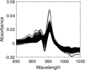
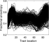
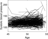
Figure 2: first derivatives of meat spectrometric curves (left panel), fractional anisotropy profiles (middle panel), and systolic blood pressure over time (right panel).

The second example studies the relationship between cognitive function and brain microstructure in the corpus callosum of patients with multiple sclerosis, a common demyelinating disease caused by inflammation in the brain. Demyelination refers to the damage to myelin that protects axons and helps nerve signal to travel faster. It occurs in the white matter of the brain and can potentially lead to loss of mobility or even cognitive impairment (Jongen et al., 2012). Diffusion tensor imaging, a technique that can produce high-resolution images of white matter tissues by tracing water diffusion within the tissues, is an important method to examine potential myelin damage in the brain. For example, from such images, some properties of white matter, such as fractional anisotropy of water diffusion, can be derived. It has been shown that fractional anisotropy is related to multiple sclerosis (Ibrahim et al., 2011).

To predict cognitive performance based on fractional anisotropy profiles, we utilize the data collected at Johns Hopkins University and the Kennedy-Krieger Institute. The data contains $n=340$ profiles from multiple sclerosis patients and paced auditory serial addition test scores that quantify cognitive function (Gronwall, 1977), where each profile was recorded at a grid of 93 points. In the middle panel of Figure 2, we show all fractional anisotropy profiles, and observe that the data is considerably more complex than the spectrometric data. The average of estimated intrinsic dimensions is 5.82 with a standard error 0.098. By contrast, the average number of principal components for functional linear regression is 11.98 with a standard error 5.22. According to Table 5, our method enjoys the most accurate prediction, while all other functional nonparametric methods deteriorate substantially.

Our third example concerns systolic blood pressure of healthy men using an anonymous data from the Baltimore longitudinal study of aging. In the study, 1590 healthy male volunteers were scheduled to visit the Gerontology Research Center bi-annually. Systolic blood pressure and current age were recorded during each visit. The design of the data is sparse and irregular, as many visits were missed by participants or not on the schedule; see Pearson et al. (1997) for more details. Our study aims to predict the average systolic blood pressure in late middle age, between 55 and 60, based on the blood pressure trajectory between age 45 and 55. By excluding subjects with at most one visit between age 45 and 55 and no visit between 55 and 60, we obtain a subset of the data with $n=323$ subjects and on average 4.2 visits per subject, shown in the right panel of Figure 2. The average of estimated intrinsic dimensions is 2.4 with a standard error 0.069, while the average number of principal components for functional linear regression is 4 with a standard error 2.01. Based on Table 5, our method outperforms others significantly.

Results for real data anslysis FLR FNW FCE FMO FCM MUL FREM MSP $2.56\,{(0.43)}$ $2.42\,{(0.33)}$ $1.97\,{(0.35)}$ $2.66\,{(0.46)}$ $2.82\,{(0.45)}$ $2.31\,{(0.35)}$ $1.06\,{(0.34)}$ DTI $1.14\,{(0.09)}$ $1.28\,{(0.12)}$ $1.36\,{(0.13)}$ $1.78\,{(0.16)}$ $1.25\,{(0.14)}$ $1.33\,{(0.13)}$ $0.96\,{(0.09)}$ SBP $1.34\,{(0.18)}$ $1.57\,{(0.17)}$ $1.64\,{(0.16)}$ $2.33\,{(0.26)}$ $1.68\,{(0.19)}$ $1.76\,{(0.17)}$ $1.15\,{(0.11)}$ FLR, functional linear regression; FNW, functional Nadaraya–Watson smoothing; FCE, functional conditional expectation; FMO, functional mode, FCM, functional conditional median; MUL, multi-method; MSP, meat spectrometric data; FREM, the proposed functional regression on manifold; DTI, diffusion tensor imaging data; SBP, systolic blood pressure data. The numbers outside of parentheses are the Monte Carlo average of root mean square error based on 100 independent simulation replicates, and the numbers in parentheses are the corresponding standard error. The results for the diffusion tensor imaging data and systolic blood pressure data are scaled by 0.1 for visualization.

Supplementary material

Additional details and simulation studies for sparse functional data, the proofs of main theorems, auxiliary results, and technical lemmas with proofs are collected in an online Supplementary Material for space economy.

See supplementary.pdf

References

- Aswani et al. (2011) Aswani, A., Bickel, P. & Tomlin., C. (2011). Regression on manifolds: Estimation of the exterior derivative. The Annals of Statistics 39, 48–81.
- Bhattacharya & Lin (2017) Bhattacharya, R. & Lin, L. (2017). Omnibus CLTs for Fréchet means and nonparametric inference on non-Euclidean spaces. Proceedings of the American Mathematical Society 145, 413–428.
- Bhattacharya & Patrangenaru (2003) Bhattacharya, R. & Patrangenaru, V. (2003). Large sample theory of intrinsic and extrinsic sample means on manifolds. I. The Annals of Statistics 31, 1–29.
- Bhattacharya & Patrangenaru (2005) Bhattacharya, R. & Patrangenaru, V. (2005). Large sample theory of intrinsic and extrinsic sample means on manifolds. II. The Annals of Statistics 33, 1225–1259.
- Cai & Yuan (2011) Cai, T. & Yuan, M. (2011). Optimal estimation of the mean function based on discretely sampled functional data: Phase transition. The Annals of Statistics 39, 2330–2355.
- Cardot et al. (1999) Cardot, H., Ferraty, F. & Sarda, P. (1999). Functional linear model. Statistics & Probability Letters 45, 11–22.
- Cardot & Sarda (2005) Cardot, H. & Sarda, P. (2005). Estimation in generalized linear models for functional data via penalized likelihood. Journal of Multivariate Analysis 92, 24–41.
- Chen & Müller (2012) Chen, D. & Müller, H. (2012). Nonlinear manifold representations for functional data. The Annals of Statistics 40, 1–29.
- Cheng & Wu (2013) Cheng, M. & Wu, H. (2013). Local linear regression on manifolds and its geometric interpretation. Journal of the American Statistical Association 108, 1421–1434.
- Coifman et al. (2005) Coifman, R., Lafon, S., Lee, A. B., Maggioni, M., Nadler, B., Warner, F. & Zucker, S. W. (2005). Geometric diffusions as a tool for harmonic analysis and structure definition of data: Diffusion maps. PNAS 102, 7426–7431.
- Cornea et al. (2017) Cornea, E., Zhu, H., Kim, P. & Ibrahim, J. G. (2017). Regression models on Riemannian symmetric spaces. Journal of the Royal Statistical Society: Series B (Statistical Methodology) 79, 463–482.
- Dai & Müller (2018) Dai, X. & Müller, H.-G. (2018). Principal component analysis for functional data on Riemannian manifolds and spheres. Annals of Statistics 46, 3334–3361.
- Delaigle & Hall (2010) Delaigle, A. & Hall, P. (2010). Defining probability density for a distribution of random functions. The Annals of Statistics 38, 1171–1193.
- Fan (1992) Fan, J. (1992). Design-adaptive nonparametric regression. Journal of the American Statistical Association 87, 998–1004.
- Fan (1993) Fan, J. (1993). Local linear regression smoothers and their minimax efficiencies. The Annals of Statistics 21, 196–216.
- Fan & Gijbels (1996) Fan, J. & Gijbels, I. (1996). Local Polynomial Model ling and Its Applications. London: Chapman and Hall.
- Ferraty et al. (2012) Ferraty, F., Keilegom, I. V. & Vieu, P. (2012). Regression when both response and predictor are functions. Journal of Multivariate Analysis 109, 10–28.
- Ferraty & Vieu (2006) Ferraty, F. & Vieu, P. (2006). Nonparametric Functional Data Analysis: Theory and Practice. New York: Springer-Verlag.
- Gronwall (1977) Gronwall, D. M. A. (1977). Paced auditory serial-addition task: A measure of recovery from concussion. Perceptual and Motor Skills 44, 367–373.
- Hall & Keilegom (2007) Hall, P. & Keilegom, I. V. (2007). Two sample tests in functional data analysis starting from discrete data. Statistica Sinica 17, 1511–1531.
- Hall & Marron (1997) Hall, P. & Marron, J. S. (1997). On the shrinkage of local linear curve estimators. Statistics and Computing 516, 11–17.
- Hall et al. (2006) Hall, P., Müller, H.-G. & Wang, J.-L. (2006). Properties of principal component methods for functional and longitudinal data analysis. The Annals of Statistics 34, 1493–1517.
- Huckemann et al. (2010) Huckemann, S., Hotz, T. & Munk, A. (2010). Intrinsic shape analysis: Geodesic PCA for Riemannian manifolds modulo isometric Lie group actions. Statistica Sinica 20, 1–58.
- Ibrahim et al. (2011) Ibrahim, I., Tintera, J., Skoch, A., F., J., P., H., Martinkova, P., Zvara, K. & Rasova, K. (2011). Fractional anisotropy and mean diffusivity in the corpus callosum of patients with multiple sclerosis: the effect of physiotherapy. Neuroradiology 53, 917–926.
- Jongen et al. (2012) Jongen, P., Ter Horst, A. & Brands, A. (2012). Cognitive impairment in multiple sclerosis. Minerva Medica 103, 73–96.
- Kudraszow & Vieu (2013) Kudraszow, N. L. & Vieu, P. (2013). Uniform consistency of kNN regressors for functional variables. Statistics & Probability Letters 83, 1863–1870.
- Lang (1995) Lang, S. (1995). Differential and Riemannian Manifolds. New York: Springer.
- Lang (1999) Lang, S. (1999). Fundamentals of Differential Geometry. New York: Springer.
- Lee & Solo (1999) Lee, T. C. & Solo, V. (1999). Bandwidth selection for local linear regression: A simulation study. Computational Statistics 14, 515–532.
- Levina & Bickel (2004) Levina, E. & Bickel, P. (2004). Maximum likelihood estimation of intrinsic dimension. Advances in Neural Information 17, 777–784.
- Li & Hsing (2010) Li, Y. & Hsing, T. (2010). Uniform convergence rates for nonparametric regression and principal component analysis in functional/longitudinal data. The Annals of Statistics 38, 3321–3351.
- Lila & Aston (2016) Lila, E. & Aston, J. (2016). Smooth principal component analysis over two-dimensional manifolds with an application to neuroimaging. The Annals of Applied Statistics 10, 1854–1879.
- Lin et al. (2019) Lin, L., Mu, N., Cheung, P. & Dunson, D. (2019). Extrinsic Gaussian processes for regression and classification on manifolds. Bayesian Analysis 14, 887–906.
- Lin et al. (2016) Lin, L., Thomas, B. S., Zhu, H. & Dunson, D. B. (2016). Extrinsic local regression on manifold-valued data. Journal of the American Statistical Association 112, 1261–1273.
- Lin & Yao (2019) Lin, Z. & Yao, F. (2019). Intrinsic Riemannian functional data analysis. The Annals of Statistics 47, 3533–3577.
- Loh & Wainwright (2012) Loh, P.-L. & Wainwright, M. J. (2012). High-dimensional regression with noisy and missing data: Provable guarantees with non-convexity. The Annals of Statistics 40, 1637–1664.
- Mas (2012) Mas, A. (2012). Lower bound in regression for functional data by representation of small ball probabilities. Electronic Journal of Statistics 6, 1745–1778.
- Mukherjee et al. (2010) Mukherjee, S., Wu, Q. & Zhou, D.-X. (2010). Learning gradients on manifolds. Bernoulli 16, 181–207.
- Müller & Stadtmüller (2005) Müller, H. G. & Stadtmüller, U. (2005). Generalized functional linear models. The Annals of Statistics 33, 774–805.
- Müller & Yao (2008) Müller, H. G. & Yao, F. (2008). Functional additive models. Journal of the American Statistical Association 103, 1534–1544.
- Panaretos et al. (2014) Panaretos, V. M., Pham, T. & Yao, Z. (2014). Principal flows. Journal of the American Statistical Association 109, 424–436.
- Patrangenaru & Ellingson (2015) Patrangenaru, V. & Ellingson, L. (2015). Nonparametric Statistics on Manifolds and Their Applications to Object Data Analysis. CRC Press.
- Pearson et al. (1997) Pearson, J., Morrell, C., Brant, L., Landis, P. & Fleg, J. (1997). Age-associated changes in blood pressure in a longitudinal study of healthy men and women. Journal of Gerontology: Medical Sciences 52, 177–183.
- Peng & Müller (2008) Peng, J. & Müller, H.-G. (2008). Distance-based clustering of sparsely observed stochastic processes, with applications to online auctions. The Annals of Applied Statistics 2, 1056–1077.
- Ramsay & Silverman (2002) Ramsay, J. O. & Silverman, B. (2002). Applied Functional Data Analysis: Methods and Case Studies. New York: Springer.
- Ramsay & Silverman (1997) Ramsay, J. O. & Silverman, B. W. (1997). Functional Data Analysis. New York: Springer-Verlag.
- Ramsay & Silverman (2005) Ramsay, J. O. & Silverman, B. W. (2005). Functional Data Analysis. Springer Series in Statistics. New York: Springer, 2nd ed.
- Roweis & Saul (2000) Roweis, S. T. & Saul, L. K. (2000). Nonlinear dimensionality reduction by locally linear embedding. Science 290, 2323–2326.
- Seifert & Gasser (1996) Seifert, B. & Gasser, T. (1996). Finite-sample variance of local polynomials: analysis and solutions. Journal of the American Statistical Association 91, 267–275.
- Sober et al. (2019) Sober, B., Aizenbud, Y. & Levin, D. (2019). Approximation of functions over manifolds: A moving least-squares approach. arxiv .
- Su et al. (2014) Su, J., Kurtek, S., Klassen, E. & Srivastava, A. (2014). Statistical analysis of trajectories on Riemannian manifolds: Bird migration, hurricane tracking, and video surveillance. The Annals of Applied Statistics 8, 530–552.
- Tenenbaum et al. (2000) Tenenbaum, J. B., Silva, V. d. & Langford, J. C. (2000). A global geometric framework for nonlinear dimensionality reduction. Science 290, 2319–2323.
- Tsybakov (2008) Tsybakov, A. B. (2008). Introduction to Nonparametric Estimation. New York: Springer.
- van der Maaten & Hinton (2008) van der Maaten, L. & Hinton, G. (2008). Visualizing data using t-SNE. Journal of Machine Learning Research 9, 2579–2605.
- Wu & Wu (2018) Wu, H.-T. & Wu, N. (2018). Think globally, fit locally under the manifold setup: Asymptotic analysis of locally linear embedding. The Annals of Statistics 46, 3805–3837.
- Yao & Müller (2010) Yao, F. & Müller, H. G. (2010). Functional quadratic regression. Biometrika 97, 49–64.
- Yao et al. (2005a) Yao, F., Müller, H.-G. & Wang, J.-L. (2005a). Functional data analysis for sparse longitudinal data. Journal of the American Statistical Association 100, 577–590.
- Yao et al. (2005b) Yao, F., Müller, H. G. & Wang, J.-L. (2005b). Functional linear regression analysis for longitudinal data. The Annals of Statistics 33, 2873–2903.
- Yao & Zhang (2019+) Yao, Z. & Zhang, Z. (2019+). Principal boundary on riemannian manifolds. Journal of the American Statistical Association , to appear.
- Yuan & Cai (2010) Yuan, M. & Cai, T. T. (2010). A reproducing kernel Hilbert space approach to functional linear regression. The Annals of Statistics 38, 3412–3444.
- Yuan et al. (2012) Yuan, Y., Zhu, H., Lin, W. & Marron, J. S. (2012). Local polynomial regression for symmetric positive definite matrices. Journal of Royal Statistical Society: Series B (Statistical Methodology) 74, 697–719.
- Zhang & Wang (2016) Zhang, X. & Wang, J.-L. (2016). From sparse to dense functional data and beyond. The Annals of Statistics 44, 2281–2321.
- Zhou & Pan (2014) Zhou, L. & Pan, H. (2014). Principal component analysis of two-dimensional functional data. Journal of Computational and Graphical Statistics 23, 779–801.