NUMERICAL SIMULATIONS OF PARTICLE ACCELERATION AT INTERPLANETARY QUASI-PERPENDICULAR SHOCKS
Abstract
Using test particle simulations we study particle acceleration at highly perpendicular () shocks under conditions of modeling magnetic turbulence. We adopt a backward-in-time method to solve the Newton-Lorentz equation using the observed shock parameters for quasi-perpendicular interplanetary shocks, and compare the simulation results with /EPAM observations to obtain the injection energy and timescale of particle acceleration. With our modeling and observations we find that a large upstream speed is responsible for efficient particle acceleration. Our results also show that the quasi-perpendicular shocks are capable of accelerating thermal particles to high energies of the order of MeV for both kappa and Maxwellian upstream distributions, which may originate from the fact that in our model the local background magnetic field has a component parallel to the shock normal.
1 INTRODUCTION
Many energetic particle events in space are associated with the acceleration at collisionless shocks (e.g., Heras et al., 1992; Kallenrode & Wibberenz, 1997; Zank et al., 2000; Li et al., 2003; Rice et al., 2003; Wang et al., 2012; Qin et al., 2013; Qi et al., 2017). The most popular theory for charged-particle acceleration is diffusive shock acceleration (DSA) (Krymsky, 1977; Axford et al., 1977; Bell, 1978; Blandford & Ostriker, 1978), which is capable to predict a power-law distribution downstream of the shock with a spectral exponent that depends only on the density compression ratio. It is widely accepted that this theory explains many important energetic particle events related to collisionless shocks. However, the energy spectra observed in space are not always in agreement with the prediction of DSA theory. In some cases, the observed energy spectra have exponential-like rollovers at higher energies (Ellison & Ramaty, 1985). The reason for the spectra rollovers is related to the losses of particles, limited acceleration time, or complicated shock geometries, all of which are not considered in the basic diffusive theory.
The angle between the shock normal and the upstream magnetic field, , is one of the most important effects that control the injection of particles at shocks. For quasi-parallel shocks, thermal particles can move along the magnetic field lines easily to cross the shock front repeatedly, so that they can be accelerated to higher energies (Ellison, 1981; Quest, 1988; Scholer, 1990; Giacalone et al., 1992). In contrast, the acceleration of thermal particles at quasi-perpendicular shocks is more difficult to be understood because particles tied to the magnetic field lines nearly parallel to the shocks can be convected across the shock to downstream. Many theoretical works have been devoted to the well-known injection problem at quasi-perpendicular shocks. In earlier studies, Ellison et al. (1995) showed that thermal particles could be accelerated by quasi-perpendicular shocks, but the acceleration efficiency decreases with increasing shock-normal angle. Using hybrid simulations, Giacalone & Ellison (2000) and Giacalone (2003) also found that quasi-perpendicular shocks did not accelerate particles efficiently. Subsequently, Giacalone (2005) performed large-scale self-consistent plasma simulations and demonstrated that thermal particles could be accelerated by perpendicular shocks. It is assumed that with large-scale magnetic fluctuations, the particles tied to meandering magnetic field lines can experience multiple crossings of the shock front, and thus be diffusively accelerated.
Recently, the injection mechanisms of shock acceleration are investigated. The injection energy can be derived from diffusion models assuming small anisotropy in the particle distribution (Giacalone & Jokipii, 1999; Giacalone & Kóta, 2006; Zank et al., 2006). Neergaard Parker & Zank (2012) and Neergaard Parker et al. (2014) explored the injection energy at quasi-parallel and quasi-perpendicular shocks, respectively, through solving the steady-state transport equation. For quasi-parallel shocks, it is suggested that the injection energy is small so an upstream Maxwellian distribution is sufficient to provide the particle injection for DSA (Neergaard Parker & Zank, 2012). The Maxwellian distribution has the form
| (1) |
where is the upstream particle (solar wind proton) number density, is the mass of a proton, is Boltzmann’s constant, is the temperature of the distribution, is the proton momentum, and corresponds to the solar wind momentum in the spacecraft frame. But for quasi-perpendicular shocks the injection energy is assumed to be large. In addition, it is known for quasi-perpendicular shocks that all reflected ions can return to the shock front and form a suprathermal population in the upstream region, and that a kappa distribution with an enhanced tail of energetic particles is demonstrated to provide an appropriate particle injection for DSA (Neergaard Parker et al., 2014). The kappa distribution can be written as
| (2) |
In this paper, we perform test particle simulations of particle acceleration associated with quasi-perpendicular interplanetary shocks with modeling magnetic turbulence by numerically solving the Newton-Lorentz equation with a backward-in-time method to clarify the crucial shock features that are responsible for efficient particle acceleration. In Section 2, we describe the shock model and numerical methods. The numerical results are shown in Section 3. We present in Section 4 the conclusions and discussion.
2 MODEL
Our numerical simulations, performed by using the code from Zhang et al. (2017) to solve the Newton-Lorentz equation to obtain the trajectories of particles in the shock frame of reference, are similar to those of Decker & Vlahos (1986a, b) except that we here consider a two-component magnetic turbulence model (described below). The Newton-Lorentz equation for a test particle in the electric field and magnetic field is given by
| (3) |
where is the particle momentum, is the particle velocity, is the particle charge, is time, and the frame of reference is moving with the shock front. The convective electric field is , with the plasma flow speed. We consider a planar, fast-mode, collisionless shock with the geometry illustrated in Figure 1. The shock is located at , and plasma flows in the positive -direction with the speeds and in the upstream and downstream regions as measured in the shock frame of reference, respectively. In the shock transition the plasma speed is given by
| (4) |
here, is the thickness of the shock transition which is assumed to be small enough compared to the gyro-radii of particles in the magnetic field, and is the compression ratio. The magnetic field is taken to be time independent as
| (5) |
where is the uniform background field, is a zero-mean turbulent field being transverse to , and a Cartesian coordinate system is adopted with -axis to be parallel to the mean magnetic field . The turbulent magnetic fluctuations are composed of a slab component and a 2D one (Matthaeus et al., 1990; Zank & Matthaeus, 1992; Bieber et al., 1996; Gray et al., 1996; Zank et al., 2006),
| (6) |
where both the two components are perpendicular to the large-scale background magnetic field , and have Kolmogorov’s spectra with a power index at high wave-number . The slab component is created with fast Fourier transform (FFT) in a box with size along the mean magnetic field and number of grids , where is the correlation scale of the slab component and is set to be AU at AU. The 2D component is created with FFT in a two-dimensional box with the correlation scale length , the 2D box size , and the number of grids . We take the ratio of magnetic energy densities of different components in the turbulence to be . For more details on the slab-2D magnetic field model, see Qin et al. (2002a, b), Qin (2002), and Zhang et al. (2017). Note that the bulk velocity and mean magnetic field satisfy the Rankine-Hugoniot (RH) conditions, but we do not consider RH for the magnetic turbulence for simplicity based on the small level and zero average of turbulence.
In the diffusive shock acceleration model, energetic particles can gain energy by crossing the shock back and forth because of the magnetic field turbulence scatterings. In this work we adopt the time-backward method to calculate the trajectories of a large number () of test particles, which are released with the same target energy measured in the spacecraft frame at the shock front. Note that varies from to in different events. Each particle orbit is followed with numerical calculations by a fourth-order Runge-Kutta method with an adjustable time step which maintains accuracy of the order of until the test particle’s motion time is up to the preset time boundary . At the time boundary, the particles have different energy (with the corresponding momentum ), most of which are lower than the target energy with the time-backward calculation because of shock acceleration. In addition, a few number () of particles with lower than a preset energy which is larger than that associated with the background plasma speed, are abandoned. Since is much smaller than , the fact that we abandon the particles does not affect the simulation results. Note that our simulation box is large enough to ensure particles not to escape the acceleration region, so the spatial boundary is not taken into account. We consider eight target energies according to the energy channels in the range (47–4750) keV from the Low-Energy Magnetic Spectrometer 30 (LEMS30) and LEMS120 detectors in the Electron, Proton, and Alpha Monitor (EPAM) instruments onboard the spacecraft. For each of the target energies we consider target pitch angle cosine with an uniform distribution in the spacecraft frame, so the distribution function at the shock front is obtained from an initial upstream background distribution function through
| (7) |
where identifies the channels of energy, indicates the boundary momentum of the test particle, and denotes the number of injected particles that contribute to the statistics. The corresponding accelerated energy spectrum is given by
| (8) |
For the upstream background distribution of energetic particles we choose the kappa distribution as shown in Equation (2), and we also choose the Maxwellian distribution as shown in Equation (1) for the comparison.
In our work for each of the shock events with the preset energy , we gradually increase the preset simulation time until the accelerated particle energy spectra do not change obviously, and we thus obtain steady-state spectra and the acceleration time . We then obtain the injection energy from the best to fit steady-state spectra from simulations with EPAM observations. The process for the fit is done by examining the dependence of the target energy spectrum on the injection energy, and in our simulaitons the injection energy error is up to the adopted steps of 0.1 keV and 0.01 keV for kappa and Maxwellian distributions, respectively.
Our model adopts test particle method, so energetic particles do not affect shock waves and magnetic fields. In addition, We adopt a particle-splitting algorithm to improve the statistics of the accelerated particles. This method has been used in previous studies by Giacalone et al. (1992). In our present time-backward simulations, when the energy of a particle drops below a preset threshold (0.75 of the initial energy), two new particles are created at the location of the mother particle with slight velocity vector deviation. The weight of the split particles is one half of the weight of the mother particle prior to the split.
Next, we describe the turbulence level settings. In Neergaard Parker et al. (2014) the steady-state diffusion transport equation was solved, and in Giacalone (2015) the time-dependent transport equation was solved by using a diffusion coefficient corresponding to a turbulence level which is significantly larger than that observed. There is a general idea that the turbulence would be enhanced when the position is close to the shock front. In this work, we employ a decaying turbulence level model from the shock front which has the form
| (9) |
where , , , are the parameters assumed according to magnetic turbulence variations, is the fitting parameter varying with different events, and to make continuous at . For simplicity, we assume for different events that parameters , , , , and do not change, with being the only variable. We use s averaged observation data of as a function of time from the Magnetometer Instrument (MAG) onboard preceding and following the shock arrival during different events, where positive and negative indicate the time after and before the shock front crossing, respectively. Here we assume as a function of which is the distance to the shock front with , where is the shock speed in the spacecraft frame.
3 DATA
Because the main ingredient in the accelerated ions from EPAM observations are protons, we only consider proton acceleration at shocks. We select SEP events observed at 1 AU during 1998-2005 at quasi-perpendicular shocks with that are identified from the shock lists provided by the ACE Web site (http://www.ssg.sr.unh.edu/mag/ace/ACElists/obs_list.html). In this work we only include quasi-perpendicular forward shocks where there was no additional shock within the previous 20 hours by following Neergaard Parker et al. (2014).
Firstly, similar to Neergaard Parker et al. (2014), we construct the upstream kappa particle distribution with using density, velocity, and temperature values obtained by averaging the five data points from the 64 s averaged data from the Solar Wind Electron, Proton, Alpha Monitor (SWEPAM) instrument onboard ahead of the shock arrival, as listed in Table 1. Secondly, we construct a Maxwellian distribution as shown in Equation (1) with density, velocity, and temperature derived from observed plasma parameters for modeling the upstream particle distribution.
Comparing MAG data onboard for different shock events and the decaying turbulence level model with Equation (9), we get the parameters km, and . In addition, we get for each event. In Figure 2, we plot the /MAG observations of the magnetic field and the ratio of the root mean square (rms) value to the total magnetic field during a representative shock event on 1998 August 26. It is shown that there is an abrupt jump of at the time of the shock passage. Besides the data from spacecraft, we also plot the results from our model with Equation (9). Table 2 summarizes the input parameters of the shock events selected, such as the shock obliquity , shock speed , upstream speed , Mach number , compression ratio , upstream magnetic field strength , the turbulence parameter , and the upstream convective electric field. The upstream background magnetic field is from seconds averaged data of MAG onboard .
4 SIMULATION RESULTS
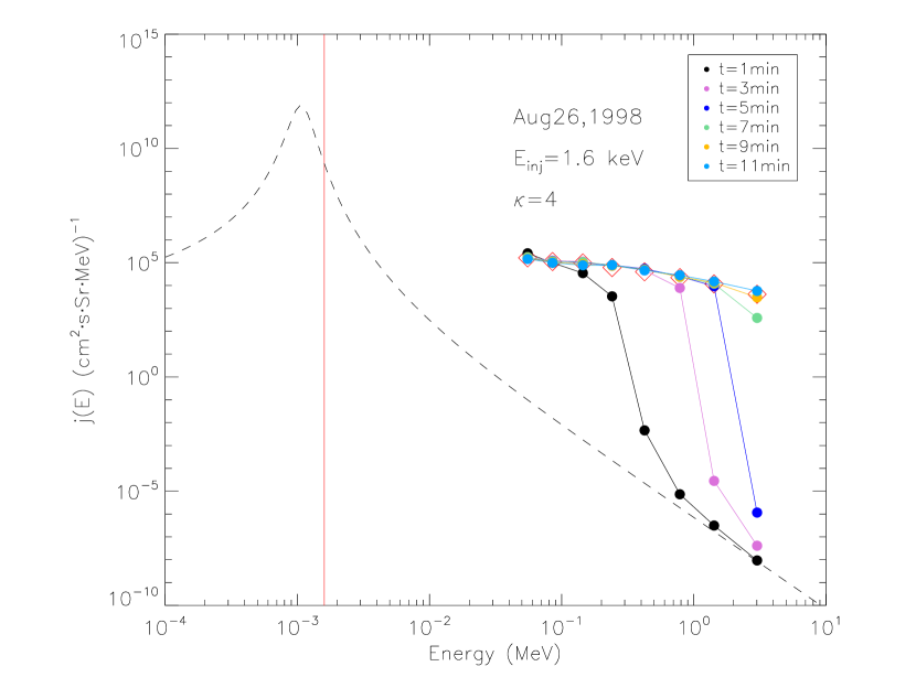
We first present the result for the event that occurred on 1998 August 26. Figure 3 shows the accelerated energy spectra from simulations with the increasing of the acceleration time (colored solid circles) along with -minute sector averages (red diamonds) of /EPAM LEMS30 and LEMS120 data taken immediately after the shock. The dashed curve shows the original upstream kappa distribution with . It is clearly seen that as the time increases the accelerated spectrum is gradually hardened, and after about minutes, the spectrum reaches the steady state which is in good agreement with the observation, we thus assume the acceleration time of this event to be minutes. It is noted that the injection energy for this event is 1.6 keV indicated by the vertical red line in Figure 3.
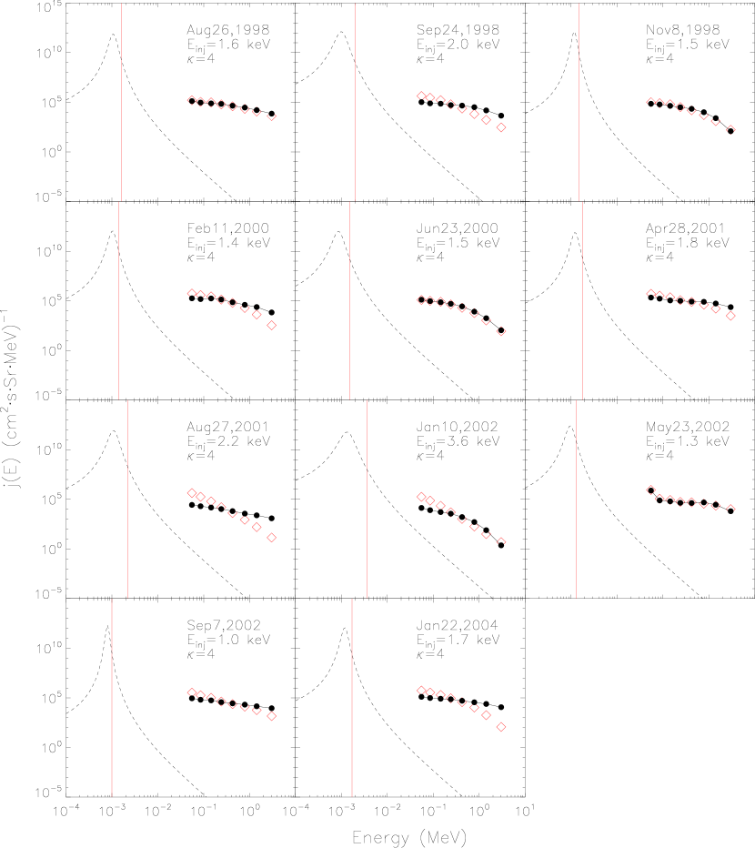
Similarly, we can get the acceleration time and injection energy for all of the quasi-perpendicular shock events. Figure 4 shows the accelerated energy spectra at the shock front for all of the shock events with hour. The black solid circles are the accelerated energy spectra from simulations with EPAM observations (red diamonds) overlaid. For the four events occurring on 1998 August 26, 1998 November 8, 2000 June 23, and 2002 May 23, the accelerated spectra fit well with the observations. However, for the rest seven cases, the simulated energy spectra are harder than the observations. These results indicate that our model is very efficient in accelerating particles with energies from a few tens of keV to several MeV.
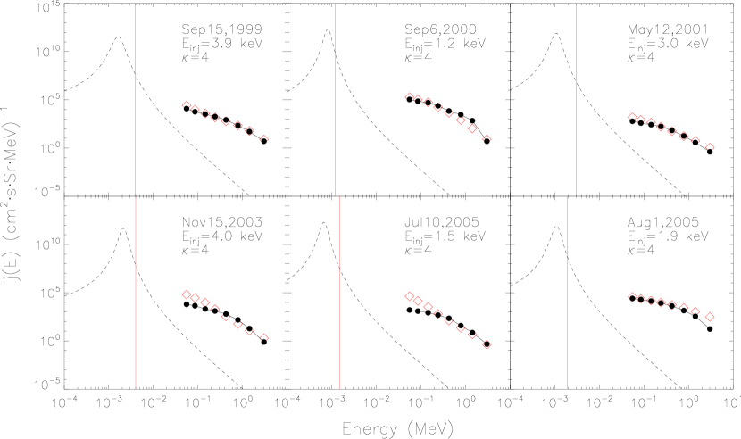
Figure 5 is similar as Figure 4 except that the shock events are with the acceleration time ranging from to hours. The accelerated energy spectra from simulations for these events are in general fit well with the observed spectra. As can be seen, the 1999 September 15 and the 2001 May 12 events show the best agreement between simulations and observations. It is worth noting that the obviously slower upstream speeds of these events, which are within 130–200 km s-1, compared to those of most shocks in the first subcategory are responsible for the longer acceleration time.
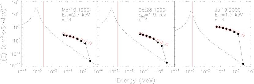
We also simulated a number of shock events with even slower upstream speeds which are about tens of kilometers per second and found that all of these shocks are very difficult to accelerate particles to higher energies within hours. In principle, simulations should be performed for the time long enough with an upper limit of several days considering the finite age of interplanetary shocks. However, we here set an upper limit of acceleration time of hours, i.e., a hours cutoff exactly, in the simulations to ensure the single shocks in our model. We list three representative examples in Table 2 and plot the simulated results in Figure 6. From Figure 6 we can see that all of the three shocks do not have the ability to accelerate particles to energies of MeV with the acceleration time of hours, therefore, all of their acceleration time hours.
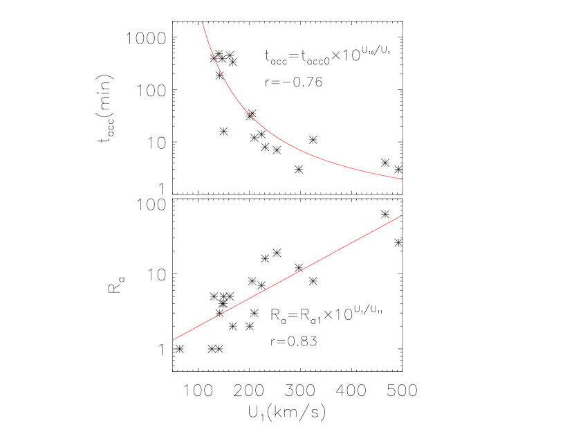
For all shock events, the acceleration time with the shock obliquities and upstream speeds are shown in Table 3. We plot the relationship between and for the events with hours in the top panel of Figure 7 as asterisks. The red curve in top panel of Figure 7 shows the fitting to an inverse proportional function in log-linear space with the form
| (10) |
where minutes, km s-1, and the correlation coefficient, . The fact that indicates a negative correlation between the acceleration time and the upstream speed. For the shock events with larger than km s-1, is less than 1 hour, while for most events with in the range of 130–200 km s-1, is in the range of 1–20 hours. The shocks with even lower , such as those during the 1999 March 10 and 1999 October 28 events, are found not capable of accelerating sufficient particles to high energies within hours.
There are some individual events deviating from the general trend discussed above, as the observed shock events are very complicated and the acceleration time can be affected by many shock parameters such as the shock-normal angle, upstream speed, magnetic field strength, compression ratio and so on. The shock occurred on 2001 August 27, which is classified into subcategory 1 as shown in Figure 4, has minutes but an upstream speed km s-1 which is slower than km s-1. The short acceleration time for this event may be expected to be related to other factors, such as the shock obliquity discussed below. This shock has a normal angle of , which is very close to and may compensate for the low to result in 1 hour. On the other hand, there are some events in subcategory 2 with around km s-1 and 3–9∘ deviated from in which is about a couple of hours. Therefore, it is suggested that the shock geometry () also plays an important role in determining the acceleration time besides the upstream speed.
To better understand the role of upstream speed in the shock acceleration, we examine the energetic particles intensity during the shock crossing for all the shock events. Here we define a quantity from spacecraft observations as the ratio of the flux of 47–65 keV at the time of the shock crossing to the background flux which is determined from the averaged flux of 12 points around 2 hours preceding the shock arrival. The values of the flux ratio are shown in Column 7 of Table 3, and we plot the relationship between and in the bottom panel of Figure 7 as asterisks. In addition, the red line in the bottom panel of Figure 7 shows a linear fitting in log-linear space with the form
| (11) |
where , km s-1, and the correlation coefficient . It is noted that the upstream speed is not the only parameter to control particle acceleration, and as the shock event conditions are complicated with many shock parameters varying, a relatively large upstream speed does not always correspond to a relatively high flux ratio. However, we here intend to focus on the general trend between and . The fact that the correlation coefficient is large () indicates the positive correlation between and . Considering that the flux ratio is actually a measure of the shock ability for accelerating particles to high energies, the observational results with Equation (11) are well consistent with our simulation results showing a strong acceleration ability for the shocks with large upstream speeds, which can be explained from the theoretical view: assuming a fixed background magnetic field, a large upstream speed will yield a high convective electric field which contributes to a large flux at the shock crossing.
We also consider an upstream Maxwellian distribution in order for a comparison with the kappa distribution for each shock event. The injection energy and from kappa and Maxwellian distributions, respectively, are shown in Table 4. We find that in each shock event . Furthermore, most of the values of and lie within the theoretical range of 1–10 keV obtained in the condition of in Zank et al. (2006). Therefore, the Maxwellian distribution can produce an accelerated distribution that matches the data. The higher injection energy for the kappa distribution is due to the fact that it is a more appropriate representation of the suprathermal population for quasi-perpendicular shocks.
5 DISCUSSION AND CONCLUSIONS
In this paper, we perform test particle simulations of particle acceleration associated with quasi-perpendicular interplanetary shocks with modeling magnetic turbulence by solving the Newton-Lorentz equation numerically with a backward-in-time method. We identify a set of quasi-perpendicular shocks from the shock database at 1 AU from 1998 to 2005, and use the observed solar wind parameters to construct kappa and Maxwellian functions as the background upstream particle distributions (Neergaard Parker et al., 2014). By comparing the accelerated energy spectra between simulations and observations, we find that the shocks are capable of accelerating thermal particles to high energies of the order of MeV with both kappa and Maxwellian upstream particle distributions. In addition, the injection energy and timescale of particle acceleration are obtained. Through examining the relationship between the acceleration time and the parameters such as upstream speed and shock-normal angle , we clarify the crucial shock features that are responsible for efficient particle acceleration.
It it noted that our simulation results indicate that we can get accelerated energy spectra with the Maxwellian upstream distribution from quasi-perpendicular shocks. Neergaard Parker et al. (2014) also calculated accelerated distribution from the Maxwellian using the final kappa injection energy. It was shown that in many cases, the obtained accelerated distribution from the Maxwellian is slightly less than or comparable to that produced by the kappa distribution. However, in our simulations for all cases the injection energy from the Maxwellian distribution is less than that produced by the kappa distribution. This difference may originate from the fact that we used test particle simulations by solving the Newton-Lorentz equation while Neergaard Parker et al. (2014) theoretically solved the steady-state transport equation, and we adopted a turbulence model in which the local background magnetic field has a component parallel to the shock normal so the shock is not precisely quasi-perpendicular locally. Although in our simulations for the quasi-perpendicular shocks the shock normal is almost perpendicular to large scale background magnetic field, it is usually less perpendicular to the local background magnetic field, since in our magnetic turbulence model the local averaged magnetic field deviates from the large scale averaged one. Therefore the injection energy in theory of perpendicular shock acceleration should not be a problem in our model.
In the future, we plan to study the particle acceleration at quasi-parallel interplanetary shocks with the similar models as in this work.
References
- Axford et al. (1977) Axford, W. I., Leer, E., & Skadron, G. 1977, Proc. 15th ICRC, 11, 132
- Bell (1978) Bell, A. R. 1978, MNRAS, 182, 147
- Bieber et al. (1996) Bieber, J. W., Wanner, W., & Matthaeus, W. H. 1996, J. Geophys. Res., 101, 2511
- Blandford & Ostriker (1978) Blandford, R. D., & Ostriker, J. P. 1978, ApJ, 221, L29
- Decker & Vlahos (1986a) Decker, R. B., & Vlahos, L. 1986a, ApJ, 306, 710
- Decker & Vlahos (1986b) Decker, R. B., & Vlahos, L. 1986b, J. Geophys. Res., 91, 13349
- Ellison (1981) Ellison, D. C. 1981, Geophys. Res. Lett., 8, 991
- Ellison & Ramaty (1985) Ellison, D. C., & Ramaty, R. 1985, ApJ, 298, 400
- Ellison et al. (1995) Ellison, D. C., Baring, M. G., & Jones, F. C. 1995, ApJ, 453, 873
- Giacalone et al. (1992) Giacalone, J., Burgess, D., Schwartz, S. J., & Ellison, D. C. 1992, Geophys. Res. Lett., 19, 433
- Giacalone & Jokipii (1999) Giacalone, J., & Jokipii, J. R. 1999, ApJ, 520, 204
- Giacalone & Ellison (2000) Giacalone, J., & Ellison, D. C. 2000, J. Geophys. Res., 105, 12541
- Giacalone (2003) Giacalone, J. 2003, Planet. Space Sci., 51, 659
- Giacalone (2005) Giacalone, J. 2005, ApJ, 628, L37
- Giacalone & Kóta (2006) Giacalone, J., & Kóta, J. 2006, Space Sci. Rev., 124, 277
- Giacalone (2015) Giacalone, J. 2015, ApJ, 799, 80
- Gray et al. (1996) Gray, P. C., Pontius, D. H., Jr., & Matthaeus, W. H. 1996, Geophys. Res. Lett., 23, 965
- Heras et al. (1992) Heras, A. M., Sanahuja, B., Smith, Z. K., Detman, T., & Dryer, M. 1992, ApJ, 391, 359
- Kallenrode & Wibberenz (1997) Kallenrode, M. B., & Wibberenz, G. 1997, J. Geophys. Res., 102, 22311
- Krymsky (1977) Krymsky, G. F. 1977, Dokl. Akad. Nauk SSSR, 234, 1306
- Li et al. (2003) Li, G., Zank, G. P., & Rice, W. K. M. 2003, J. Geophys. Res., 108, 1082
- Matthaeus et al. (1990) Matthaeus, W. H., Goldstein, M. L., & Roberts, D. A. 1990, J. Geophys. Res., 95, 20673
- Neergaard Parker & Zank (2012) Neergaard Parker, L., & Zank, G. P. 2012, ApJ, 757, 97
- Neergaard Parker et al. (2014) Neergaard Parker, L., Zank, G. P., & Hu, Q. 2014, ApJ, 782, 52
- Qi et al. (2017) Qi, S.-Y., Qin, G., & Wang, Y. 2017, Res. Astron. Astrophys., 17, 33
- Qin (2002) Qin, G. 2002, PhD thesis, UNIVERSITY OF DELAWARE
- Qin et al. (2002a) Qin, G., Matthaeus, W. H., & Bieber, J. W. 2002a, Geophys. Res. Lett., 29, 1048
- Qin et al. (2002b) Qin, G., Matthaeus, W. H., & Bieber, J. W. 2002b, ApJ, 578, L117
- Qin et al. (2013) Qin, G., Wang, Y., Zhang, M., & Dalla, S. 2013, ApJ, 766, 74
- Quest (1988) Quest, K. B. 1988, J. Geophys. Res., 93, 9649
- Rice et al. (2003) Rice, W. K. M., Zank, G. P., & Li, G. 2003, J. Geophys. Res., 108, 1369
- Scholer (1990) Scholer, M. 1990, Geophys. Res. Lett., 17, 1821
- Wang et al. (2012) Wang, Y., Qin, G., & Zhang, M. 2012, ApJ, 752, 37
- Zank & Matthaeus (1992) Zank, G. P., & Matthaeus, W. H. 1992, J. Geophys. Res., 97, 17189
- Zank et al. (2000) Zank, G. P., Rice, W. K. M., & Wu, C. C. 2000, J. Geophys. Res., 105, 25079
- Zank et al. (2006) Zank, G. P., Li, G., Florinski, V., Hu, Q., Lario, D., & Smith, C. W. 2006, J. Geophys. Res., 111, A06108
- Zhang et al. (2017) Zhang, L.-H., Qin, G., Sun, P., & Wang, H.-N. 2017, submitted to ApJ, arXiv:1702.04647


| Date of Shock | (cm-3) | (∘ K) | (km s-1) | |||
|---|---|---|---|---|---|---|
| 1998 Aug 26 | 4.25 | 451 | ||||
| 1998 Sep 24 | 10.51 | 434 | ||||
| 1998 Nov 8 | 5.39 | 475 | ||||
| 1999 Mar 10 | 11.32 | 414 | ||||
| 1999 Sep 15 | 3.69 | 554 | ||||
| 1999 Oct 28 | 6.03 | 379 | ||||
| 2000 Feb 11 | 5.78 | 443 | ||||
| 2000 Jun 23 | 6.57 | 405 | ||||
| 2000 Jul 19 | 3.67 | 487 | ||||
| 2000 Sep 6 | 10.53 | 394 | ||||
| 2001 Apr 28 | 4.26 | 484 | ||||
| 2001 May 12 | 5.97 | 454 | ||||
| 2001 Aug 27 | 6.16 | 454 | ||||
| 2002 Jan 10 | 6.76 | 501 | ||||
| 2002 May 23 | 14.87 | 429 | ||||
| 2002 Sep 7 | 4.97 | 392 | ||||
| 2003 Nov 15 | 4.19 | 635 | ||||
| 2004 Jan 22 | 5.84 | 475 | ||||
| 2005 Jul 10 | 9.33 | 356 | ||||
| 2005 Aug 1 | 5.62 | 457 |
| Date of Shock | (km/s) | (km/s) | s | (nT) | c() | (N/C) | ||
|---|---|---|---|---|---|---|---|---|
| 1998 Aug 26 | 88 | 675 | 325 | 6.3 | 3.2 | 4.79 | 0.107 | 1.56 |
| 1998 Sep 24 | 87 | 644 | 297 | 2.9 | 3.0 | 14.67 | 0.047 | 4.35 |
| 1998 Nov 8 | 77 | 582 | 210 | 1.2 | 1.9 | 17.35 | 0.044 | 3.55 |
| 1999 Mar 10 | 78 | 522 | 127 | 3.3 | 1.5 | 5.19 | 0.047 | 0.64 |
| 1999 Sep 15 | 83 | 648 | 168 | 2.3 | 2.3 | 7.33 | 0.054 | 1.22 |
| 1999 Oct 28 | 83 | 423 | 64 | 1.2 | 1.7 | 6.84 | 0.069 | 0.43 |
| 2000 Feb 11 | 88 | 539 | 224 | 3.6 | 2.8 | 6.71 | 0.045 | 1.50 |
| 2000 Jun 23 | 85 | 483 | 201 | 3.0 | 2.5 | 8.23 | 0.055 | 1.65 |
| 2000 Jul 19 | 81 | 606 | 150 | 3.0 | 2.9 | 4.64 | 0.071 | 0.69 |
| 2000 Sep 6 | 85 | 485 | 131 | 2.3 | 2.3 | 8.73 | 0.029 | 1.14 |
| 2001 Apr 28 | 88 | 905 | 492 | 5.9 | 3.7 | 9.35 | 0.089 | 4.60 |
| 2001 May 12 | 84 | 486 | 141 | 1.2 | 1.3 | 13.09 | 0.018 | 1.84 |
| 2001 Aug 27 | 89 | 486 | 150 | 2.7 | 2.8 | 6.35 | 0.085 | 0.95 |
| 2002 Jan 10 | 75 | 643 | 206 | 3.5 | 3.0 | 10.08 | 0.087 | 2.01 |
| 2002 May 23 | 84 | 834 | 466 | 4.2 | 1.7 | 16.12 | 0.045 | 7.47 |
| 2002 Sep 7 | 89 | 628 | 231 | 2.4 | 2.9 | 8.44 | 0.061 | 1.95 |
| 2003 Nov 15 | 81 | 738 | 162 | 3.0 | 2.6 | 6.54 | 0.080 | 1.05 |
| 2004 Jan 22 | 89 | 738 | 254 | 4.2 | 3.7 | 7.14 | 0.102 | 1.81 |
| 2005 Jul 10 | 82 | 374 | 147 | 2.0 | 1.8 | 10.64 | 0.030 | 1.55 |
| 2005 Aug 1 | 87 | 496 | 142 | 1.5 | 1.9 | 6.25 | 0.051 | 0.89 |
| Date of Shock | (km/s) | (min) | (keV) | (47–65 keV) | |
|---|---|---|---|---|---|
| 1998 Aug 26 | 88 | 325 | 11 | 1.6 | 8 |
| 1998 Sep 24 | 87 | 297 | 3 | 2.0 | 12 |
| 1998 Nov 8 | 77 | 210 | 12 | 1.5 | 3 |
| 1999 Mar 10 | 78 | 127 | 1200 | 2.7 | 1 |
| 1999 Sep 15 | 83 | 168 | 336 | 3.9 | 2 |
| 1999 Oct 28 | 83 | 64 | 1200 | 1.9 | 1 |
| 2000 Feb 11 | 88 | 224 | 14 | 1.4 | 7 |
| 2000 Jun 23 | 85 | 201 | 31 | 1.5 | 2 |
| 2000 Jul 19 | 81 | 150 | 1200 | 1.5 | 4 |
| 2000 Sep 6 | 85 | 131 | 396 | 1.2 | 5 |
| 2001 Apr 28 | 88 | 492 | 3 | 1.8 | 26 |
| 2001 May 12 | 84 | 141 | 486 | 3.0 | 1 |
| 2001 Aug 27 | 89 | 150 | 16 | 2.2 | 5 |
| 2002 Jan 10 | 75 | 206 | 35 | 3.6 | 8 |
| 2002 May 23 | 84 | 466 | 4 | 1.3 | 62 |
| 2002 Sep 7 | 89 | 231 | 8 | 1.0 | 16 |
| 2003 Nov 15 | 81 | 162 | 450 | 4.0 | 5 |
| 2004 Jan 22 | 89 | 254 | 7 | 1.7 | 19 |
| 2005 Jul 10 | 82 | 147 | 390 | 1.5 | 4 |
| 2005 Aug 1 | 87 | 142 | 186 | 1.9 | 3 |
| Date of Shock | (keV) | (keV) |
|---|---|---|
| 1998 Aug 26 | 1.6 | 1.43 |
| 1998 Sep 24 | 2.0 | 1.54 |
| 1998 Nov 8 | 1.5 | 1.42 |
| 1999 Mar 10 | 2.7 | 1.40 |
| 1999 Sep 15 | 3.9 | 2.65 |
| 1999 Oct 28 | 1.9 | 1.13 |
| 2000 Feb 11 | 1.4 | 1.30 |
| 2000 Jun 23 | 1.5 | 1.26 |
| 2000 Jul 19 | 1.5 | 1.45 |
| 2000 Sep 6 | 1.2 | 1.08 |
| 2001 Apr 28 | 1.8 | 1.60 |
| 2001 May 12 | 3.0 | 1.70 |
| 2001 Aug 27 | 2.2 | 1.66 |
| 2002 Jan 10 | 3.6 | 2.38 |
| 2002 May 23 | 1.3 | 1.20 |
| 2002 Sep 7 | 1.0 | 0.93 |
| 2003 Nov 15 | 4.0 | 3.05 |
| 2004 Jan 22 | 1.7 | 1.53 |
| 2005 Jul 10 | 1.5 | 0.99 |
| 2005 Aug 1 | 1.9 | 1.55 |